Do the rich save more? Evidence from linked survey and administrative data

Abstract

The nature of the relationship between lifetime income and saving rates is a longstanding empirical question and one that has been surprisingly difficult to answer. We use a new data set containing both individual survey data on wealth holdings and administrative data on earnings histories to examine this question. We find, for a sample of English households, evidence of a positive relationship between the rate of private wealth accumulation and levels of lifetime earnings. Even when state pension wealth is included, the top quintile of lifetime earnings have significantly higher wealth to lifetime earnings ratios than the other quintiles. Under this broad measure of wealth, those in the middle of the distribution of lifetime earnings accumulate the least wealth relative to their earnings.

JEL

C81 - Methodology for Collecting, Estimating, and Organizing Microeconomic Data; Data Access D12 - Consumer Economics: Empirical Analysis D91 - Role and Effects of Psychological, Emotional, Social, and Cognitive Factors on Decision Making

Issue Section:

Articles

1. Introduction

Whether higher lifetime income households save a larger share of their income is an empirical question that has been surprisingly difficult to answer. It is surprising that no consensus has been reached on this issue both because the question is apparently simple—it is just a correlation—and because there is enormous interest in knowing this fact in order to make progress on a number of important policy issues.

One example of where this question has been much debated recently by economic researchers is in the optimal tax literature. Whether saving propensities vary systematically by permanent income level is relevant for whether capital income should be taxed. Saez (2002)—generalizing the results from Atkinson and Stiglitz (1976) to the case of heterogeneous preferences—argues that, if high ability individuals save more, taxation of capital income can be welfare improving. Diamond and Spinnewijn (2011) extend this work and highlight the importance of the relationship between the willingness to work and saving propensities, conditional on ability. The general intuition behind these results is that, if ability is unobserved but high ability individuals act in a particular way (for example, by saving a lot) then this information can be used by the tax authorities to reveal the ‘types’ of taxpayers and thus reduce the efficiency cost of a given redistributive objective.

The corresponding empirical question is, however, only apparently simple. There is no controversy about the fact that households with high current income save more than those with low current income. This is a well-established fact. But there is a lot more disagreement about whether one can conclude from this that the ‘rich’ (those with high permanent income) do indeed save more. Friedman (1953, 1957) was the first to suggest that no such conclusion can be drawn from this stylized fact. If income is varying over the life cycle, individuals should be willing to smooth their consumption by saving in good times and borrowing in bad ones. He postulated that empirical evidence available at the time he was writing could not reject that saving rates were constant across the distribution of permanent income.

The empirical difficulty is twofold: until recently, good quality microdata on either saving rates or wealth holdings has been limited; and it is difficult to measure permanent or lifetime income with most of the available data sources. It is even rarer for data sets to allow the construction of good measures of both saving rates or wealth and permanent income. Previous literature has relied mainly on two different methods to tackle this question. The first strand of the literature has used consumption and income data to measure saving and has instrumented for permanent income using education, current consumption or lagged earnings. Dynan et al. (2004), using this methodology on US data, found that the ‘rich’ do save a higher fraction of their income. A potential problem with this instrumental variables approach is the validity of the instrument. For instance, if, in addition to its impact on lifetime earnings, education has a direct impact on saving rates (for example, if it is correlated with discount rates), then the approach can be called into question, or at least lead to the results having a different interpretation. Alan et al. (2015), working with Canadian consumption data, argue that the relationship between saving rates and long-term income is flat and that the approach used by Dynan et al. (2004) is upwardly biased. In the second strand of the literature, Gustman and Steinmeier (1999) and Venti and Wise (1998, 1999, 2000) used US administrative data on earnings histories linked to the Health and Retirement Study to analyse how wealth in retirement is associated with different levels of lifetime earnings. They found that ratios of retirement wealth to lifetime earnings initially fall as lifetime earnings increase but are then roughly constant across the bulk of the lifetime income distribution, with Venti and Wise (1999) finding a very slight increase in wealth to lifetime earnings ratios for those in the top two deciles. Using Panel Study of Income Dynamics data on private wealth holdings (excluding Social Security wealth), Hendricks (2007) finds a roughly flat mean wealth to lifetime earnings ratio but increasing median wealth to lifetime earnings ratio.

In this paper, we present results using newly available information from the English Longitudinal Study of Ageing (ELSA) linked to administrative data on earnings since 1975 and employment since 1948. With these data, which have not previously been exploited, we can compute measures of lifetime earnings based on a very long panel and relate ratios of wealth to lifetime earnings to the distribution of lifetime earnings. When we use lifetime earnings per year worked as a proxy for earning ability, we find that the ratio of private wealth (i.e. wealth excluding state pension wealth) to lifetime earnings increases monotonically with lifetime earnings, consistent with the conjecture that the ‘rich save more’. Even when state pension wealth is included, the top quintile of lifetime earnings exhibits significantly higher wealth to lifetime earnings ratios than the other quintiles. Under this broad measure of wealth, those in the middle of the distribution of lifetime earnings accumulate the least wealth relative to their earnings.

Our approach is closest to that used by Gustman and Steinmeier (1999) and Venti and Wise (1998), but while these previous papers focused on explaining large wealth dispersion given lifetime earnings (a fact that our data confirm too), our methodology provides a clear test of the relationship between wealth accumulation and lifetime earnings, accounting for the taxation system as well as both the private and state pension systems.

The rest of the paper is organized as follows. Section 2 outlines a very simple version of the canonical life cycle model in which saving rates would not vary with income, before highlighting departures which could generate a relationship between saving rates (and wealth) and lifetime earnings. Section 3 describes the data that we use and outlines our empirical approach. Results are presented in Section 4. Section 5 concludes.

2. Theoretical background

Our aim is to assess whether the ‘rich’ (measured by permanent income) ‘save more’ (where saving will be proxied by ratios of wealth to lifetime earnings). We start by describing the most basic life cycle model—one whose solution implies that saving rates will not vary with earnings ability, and then discuss possible departures from that stylized model that could generate a relationship between saving and permanent income.

2.1 A simple life cycle model

Consider a setting where each individual (or household as a collective unit) maximizes his lifetime utility, U, derived from consumption (C_t) in each year of his life. Utility in each period (⁠

u (.)

⁠) is discounted by a discount rate δ, and the individual’s length of life, known with certainty, is T. Lifetime utility is equal to:

U = \sum_{t = 0}^{T} \frac{1}{{(1 + δ)}^{t}} u (C_{t})

(1)

The individual maximizes his lifetime utility subject to his lifetime budget constraint, shown in eq. (2)—which implies that the discounted value of consumption must not be more than that of net income (Y_t):

\sum_{t = 0}^{T} (\prod_{τ = t}^{T} (1 + r_{τ})) C_{t} \leq \sum_{t = 0}^{T} (\prod_{τ = t}^{T} (1 + r_{τ})) Y_{t}

(2)

where r_t is a (potentially time-varying) interest rate.

This simple model contains no bequest motive, no endogenous labour supply choices, no heterogeneity in either discount rates or in the single-period utility function, and no uncertainty over rates of returns, income or length of life. If we assume further a homothetic utility function, and that there are no constraints on borrowing or saving, optimal behaviour will be that savings—and wealth accumulated—are proportional to net lifetime income (Masson, 1988; Dynan et al., 2004). Under this framework and with these strong restrictions, lifetime resources do not matter for saving rates and the Friedman hypothesis—that saving rates have no systematic relationship with permanent income—is validated.

2.2 Departures from this model

In reality there are many departures from the very restrictive benchmark model presented above which could lead to a non-zero gradient between wealth and lifetime income.

First, preferences might vary with household characteristics—including their earnings ability. There is likely to be heterogeneity in preference for leaving bequests (Kopczuk and Lupton, 2007), rates of time preference (Samwick, 1998; Gustman and Steinmeier, 2005), preferences for leisure (Eckstein and Wolpin, 1999) and risk-aversion (Parker and Fischhoff, 2005; Frederick, 2005).

Second, the economic environment could differ by household type. Life expectancies vary with permanent income (Attanasio and Hoynes, 2000) and there is evidence that some individuals earn better rates of return than others, not simply as a reward for greater tolerance for risk but also coming from greater financial literacy (Lusardi and Mitchelli, 2007) or through the opportunities to leverage investments afforded to those who hold larger asset portfolios.

Third, uncertainty could cause differences in saving behaviour across the distribution of earnings. The model above is one in which all future realization of features of the economic environment are known with certainty. In reality, savings decisions over the life-cycle are based on expectations of income flows, consumption needs and investment returns. Introducing uncertainty in any of these (e.g. stochastic process for health, asset prices, earnings or employment opportunities) will affect wealth accumulation, quite possibly in a manner that differs across the distribution of earnings potential.¹

Fourth, tax and benefit systems can generate strong incentives for some individuals to save more than others. In particular, consumption floors (Hubbard et al., 1995) and means-tested retirement programs (Sefton et al., 2008) can discourage saving among those with low levels of wealth—a group that, regardless of heterogeneity in saving behaviour, certainly draws heavily from those with lower permanent income. Additionally, public pension programmes (such as Social Security in the US or the State Pension in the UK) essentially force individuals to accumulate wealth (at a rate that, if the programme is redistributive, certainly differs by their earnings). Unless this ‘forced saving’ crowds out an exactly equal quantity of private saving, correlations between a broad measure of wealth and its ratio with lifetime earnings will result.

The aim of this paper is not to assess the relationship between each of these factors and lifetime earnings but rather to assess their net effect. That is, we address the question: taking the effect of the differences in preferences, the economic environment as well as tax, benefit and public pension systems together, what is the relationship between the rate of wealth accumulation and lifetime earnings?

3. Methodology and data

3.1 Empirical approach

Our empirical approach relies on assessing the relationship between earnings ability and the ratio of wealth to lifetime earnings. We examine a measure of the ratio of wealth holdings in a year close to the end of working life (given by year X below) to net lifetime earnings (⁠

\frac{W_{i}^{X}}{N L E_{i}}

⁠) and examine how this is related to measures of earning ability (E_i).

W_{i}^{X}

is wealth accumulated by the year X. In our empirical application we will consider a number of definitions of wealth: the broadest will be the sum of all private wealth and state pension wealth (the UK’s public pension is typically known as the ‘state pension’ and we use that term here). Net lifetime earnings are the present value of net real earnings between the start of working life and age X:

N L E_{i} = \sum_{t = 0}^{X} (\prod_{τ}^{X} (1 + r_{τ}) (1 + π_{τ})) Y_{i t}

(3)

where Y_it is nominal net-of-tax earnings in period t for individual i, π is the rate of inflation (and so ensures that all earnings enter NLE in real, year X, prices) and r is a real rate of return. This differs from the simpler present-value calculation in eq. (2) by the necessity of converting from current to present period prices (the model abstracted from inflation). The real rate of return (r) that we use to do the present value calculation is the rate of growth of economy-wide real earnings. This, proxying for the rate of growth of the economy, is designed to capture the rate of return on a broad portfolio of wealth (which comprises cash, risky assets, pension wealth, entitlements under the state pension system, housing as well as other forms of wealth).²

Earnings ability for an individual i (E_i) is measured as their net lifetime resources divided by their number of years in work (n_i):

E_{i} = \frac{N L E_{i}}{n_{i}}

(4)

We use earnings per year worked rather than total earnings as our measure of earnings ability to avoid voluntary periods out of the labour market (early retirement, for example) depressing measured earnings ability. It has the disadvantage, however, that involuntary periods out of the labour market, which are genuinely indicative of diminished earnings ability, do not have this effect reflected in E.³ For comparison, we provide results where we use total earnings rather than earnings per year as our measure of earnings ability—and the results in both cases are very similar.

Equation (5) gives our primary empirical equation which is estimated using median regressions:

\frac{W_{i}^{R}}{N L E_{i}} = f (E_{i}) + X_{i} β + ϵ_{i t}

(5)

We specify the function $f ()$ in eq. (5) as a set of quantile dummies to allow for a non-linear (and potentially non-monotonic) association between wealth and earnings ability. X is a vector of covariates, which, in our main specification will contain a set of age dummies only.

3.2 Data

The data we use is a newly available data set based on the linkage of the English ageing survey, ELSA, to administrative data from the UK National Insurance (NI) system. We discuss each in turn.

ELSA is a biennial longitudinal survey of a representative sample of the English household population aged 50 and over (plus their partners). The first wave was conducted between April 2002 and March 2003 and sampled 11,391 individuals from 7,934 households. ELSA collects a wide range of information on individuals’ circumstances. This includes detailed measures of their financial situation: income from all sources (including earnings, self-employment income, benefits and pensions), non-pension wealth (including the type and amount of financial assets, property, business assets and antiques) and private pension wealth (including information on past contributions and details of current scheme rules). ELSA also collects information on individuals’ physical and mental health, cognitive ability, social participation and expectations of future events (such as surviving to some older age or receiving an inheritance). As complements to our main results, we explore below some interesting associations between wealth accumulation and some of these variables.

ELSA has been linked to NI records, which are administrative data collected by the UK government since 1948 in order to keep track of individuals’ contributions to the social insurance system and establish their entitlement to benefits, such as state pensions.⁴ ELSA respondents were asked for permission to link to their NI records. Among respondents to the 2002–3 wave of ELSA, 79% gave permission for a link to be made to their NI records and 71.8% have been successfully linked. While there are differences in some dimensions between the full ELSA sample and the linked subset (in particular the very old and the self-employed are under-represented among those who agreed to allow their NI records to be linked⁵), the samples do not look very dissimilar.⁶

We extract a sub-sample from this data of couples where the oldest partner was aged between 60 and 75 at the time of their ELSA wave 1 interview in 2002/03 (and so was born between 1927 and 1942). We focus only on those in couples, rather than currently single individuals because the vast majority of single individuals in this age group had previously been married. As we only have information on the lifetime earnings of current ELSA respondents, and not those of former or late partners, there is a potentially large component of the lifetime resources for single pensioners (namely, former partners’ earnings) that is not observed in our data. There are 1,937 couples in the first wave of ELSA in which the oldest member was born between 1927 and 1942. For 1,157 of these couples we have linked administrative data on both partners’ past earnings. The NI records do not record income of the self-employed; therefore, we exclude from our analysis any couples in which one individual had more than five years in which they paid self-employed NI contributions—this results in us dropping 129 couples. Finally, there are five couples for whom we do not observe full information on wealth or the other covariates of interest. These restrictions yield a sample of 1,023 couples for which we have detailed information on both wealth at retirement and earnings during their lifetime.

We examine the relationship between lifetime earnings and a variety of wealth concepts (in 2002/3)⁷. First, we measure total private wealth excluding state pension wealth, including wealth from private pensions, owner-occupied housing, other property, business assets and financial assets. Wealth is the measured net of outstanding secured and unsecured debts. Second, we compute a broader measure of total wealth including state pension wealth, computed as the present discounted value of the future stream of pension income to which an individual is entitled.⁸

Turning to the construction of a measure of total lifetime earnings, while our administrative data contains rich and unexploited data, it has three limitations. First, earnings are recorded only if they were above a certain minimum level. This level, the ‘Lower Earnings Limit’ was equal to £75 per week (£3,900 a year) in our most recent year of data—and over the period covered by our microdata was normally located at about the 10th percentile of the (positive) distribution of earnings. Given this threshold is set at quite a low level, this will only marginally affect our estimates of lifetime earnings for most individuals. Second, prior to 1997 the NI data only record earnings up to a cap; this cap was equal to £585 per week (£30,420) in our more recent year of data. The censoring point varies year by year, but in most years was located close to the 90th percentile of positive gross earnings.⁹ Third, the NI records only contain details of earnings back to 1975. As the focus of this paper is individuals aged 60 to 75 in 2002–3, this means we will have earnings from age 48 for the oldest individuals in our sample and from age 34 for the youngest individuals in our sample.

To address the issue of recorded earnings being capped in the administrative data, we run a fixed-effect Tobit on earnings from 1975 to 2003 with data up to 1996 censored.¹⁰ In addition to the fixed effect, dummies for each year are included (1975 being the omitted year—a fact that will be important below in interpreting the fixed effect). Separate Tobits are run for groups defined by sex, education and cohort. There are three education groups, the two genders, and individuals are grouped into five-year birth cohorts and so, in these cohort-specific regressions the year dummies capture life cycle (age) patterns in earnings. We use the coefficients of this Tobit to predict earnings for those who are affected by the censoring.

Turning to how we deal with the absence of earnings data from prior to 1975, from the administrative data we know for how many weeks the individual made contributions between 1948 and 1975, but we do not know what his/her earnings were in those years nor when exactly he/she made the contributions. Our estimation of earnings prior to 1975 proceeds in two stages: (i) we back-cast ‘potential’ earnings in years prior to 1975 based on the fixed effect estimated using the procedure described above (which represents an estimate of ‘permanent’ earnings power expressed in 1975 prices) and assumptions about the shape of the age-earnings profile and economy-wide average earnings growth in each year; and (ii) we make an assumption about which years the individual was actually in employment based on the number of weeks of work recorded in the administrative data, and employment patterns reported in the life history data. We give further details on this in Appendix A.

The final step necessary to construct measures of both gross and net lifetime earnings is to sum earnings across all years for each benefit unit.¹¹ Recall that we up-rate earnings from the year in which they were earned to 2002 using average earnings growth.¹² Then we sum, for each family unit, all the earnings for each individual from age 16 to 64 (inclusive). For further details see Appendix A.

3.3 Descriptive statistics

Before assessing the relationship between wealth at retirement and lifetime earnings, it is worth giving a sense of the distribution of our measure of lifetime earnings. Table 1 presents average lifetime earnings by decile of lifetime earnings for couples. The deciles in this table and throughout the remainder of the paper are, unless explicitly stated, defined based on net lifetime earnings per year worked. Couples in the bottom decile earned, on average, £552,000 during their lifetime while couples in the top decile earned, on average, more than £2,726,000. The ratio of the 90th percentile to the 10th percentile is 2.6. For comparison, this ratio was 4.1 for the distribution of current income in 2002, and 3.2 in 1961 (Cribb et al., 2013)—that is there is lower inequality in lifetime earnings than in current income. The last two columns of Table 1 present average lifetime earnings per year worked (E) for couples in each decile of the lifetime earnings distribution.

Table 1

Average lifetime earnings by decile of lifetime earnings

Decile of lifetime earnings	Lifetime earnings		Lifetime earnings per year worked
	Mean	Median	Mean	Median
1	552,437	568,925	7,560	7,938
2	774,386	813,007	10,172	10,182
3	916,886	929,976	11,510	11,519
4	1,004,588	1,023,199	12,640	12,690
5	1,101,930	1,113,148	13,680	13,621
6	1,142,037	1,161,576	14,692	14,667
7	1,264,651	1,286,452	16,043	16,012
8	1,416,124	1,418,486	17,835	17,776
9	1,590,741	1,588,888	20,385	20,210
10	2,726,270	2,251,952	33,863	29,221
Total	1,248,100	1,132,685	15,827	14,208

Decile of lifetime earnings	Lifetime earnings		Lifetime earnings per year worked
	Mean	Median	Mean	Median
1	552,437	568,925	7,560	7,938
2	774,386	813,007	10,172	10,182
3	916,886	929,976	11,510	11,519
4	1,004,588	1,023,199	12,640	12,690
5	1,101,930	1,113,148	13,680	13,621
6	1,142,037	1,161,576	14,692	14,667
7	1,264,651	1,286,452	16,043	16,012
8	1,416,124	1,418,486	17,835	17,776
9	1,590,741	1,588,888	20,385	20,210
10	2,726,270	2,251,952	33,863	29,221
Total	1,248,100	1,132,685	15,827	14,208

Notes: In GBP, 2002 prices. Sample size: 1,023 couples.

Source: ELSA linked with NI records.

Table 1

Average lifetime earnings by decile of lifetime earnings

Decile of lifetime earnings	Lifetime earnings		Lifetime earnings per year worked
	Mean	Median	Mean	Median
1	552,437	568,925	7,560	7,938
2	774,386	813,007	10,172	10,182
3	916,886	929,976	11,510	11,519
4	1,004,588	1,023,199	12,640	12,690
5	1,101,930	1,113,148	13,680	13,621
6	1,142,037	1,161,576	14,692	14,667
7	1,264,651	1,286,452	16,043	16,012
8	1,416,124	1,418,486	17,835	17,776
9	1,590,741	1,588,888	20,385	20,210
10	2,726,270	2,251,952	33,863	29,221
Total	1,248,100	1,132,685	15,827	14,208

Decile of lifetime earnings	Lifetime earnings		Lifetime earnings per year worked
	Mean	Median	Mean	Median
1	552,437	568,925	7,560	7,938
2	774,386	813,007	10,172	10,182
3	916,886	929,976	11,510	11,519
4	1,004,588	1,023,199	12,640	12,690
5	1,101,930	1,113,148	13,680	13,621
6	1,142,037	1,161,576	14,692	14,667
7	1,264,651	1,286,452	16,043	16,012
8	1,416,124	1,418,486	17,835	17,776
9	1,590,741	1,588,888	20,385	20,210
10	2,726,270	2,251,952	33,863	29,221
Total	1,248,100	1,132,685	15,827	14,208

Notes: In GBP, 2002 prices. Sample size: 1,023 couples.

Source: ELSA linked with NI records.

Table 2 shows how mean total wealth and some of its components (private and state pension wealth, housing wealth and financial wealth) vary with lifetime earnings.¹³ Mean total wealth is just under £250,000 for couples in the bottom decile, compared to £1,070,000 in the top decile. Unsurprisingly, private pension wealth exhibits a strong positive relationship with the level of lifetime earnings. Financial wealth is very concentrated in the top two deciles of the lifetime earnings distribution, while housing wealth is much more evenly distributed. State pension wealth, on the other hand, is flat across the lifetime earnings distribution. It reflects the broadly flat-rate nature of state pensions in the UK.¹⁴

Table 2

Mean wealth measures by decile of lifetime earnings

Decile of lifetime earnings	Total wealth	Private pension wealth	State pension wealth	Housing wealth	Net financial wealth
1	249,995	45,642	116,857	61,959	18,838
2	325,460	81,582	113,677	90,680	28,047
3	342,299	81,975	117,590	99,404	34,643
4	338,867	96,678	113,647	99,374	22,134
5	395,947	122,159	105,647	100,053	36,177
6	465,060	160,528	110,808	133,166	42,291
7	449,036	150,035	118,429	118,584	44,021
8	619,859	257,284	115,577	162,939	61,457
9	707,459	275,184	113,961	190,258	82,517
10	1,070,170	420,633	137,385	283,851	142,514
Total	495,974	168,960	116,358	133,908	51,197

Decile of lifetime earnings	Total wealth	Private pension wealth	State pension wealth	Housing wealth	Net financial wealth
1	249,995	45,642	116,857	61,959	18,838
2	325,460	81,582	113,677	90,680	28,047
3	342,299	81,975	117,590	99,404	34,643
4	338,867	96,678	113,647	99,374	22,134
5	395,947	122,159	105,647	100,053	36,177
6	465,060	160,528	110,808	133,166	42,291
7	449,036	150,035	118,429	118,584	44,021
8	619,859	257,284	115,577	162,939	61,457
9	707,459	275,184	113,961	190,258	82,517
10	1,070,170	420,633	137,385	283,851	142,514
Total	495,974	168,960	116,358	133,908	51,197

Notes: In GBP, 2002 prices. Sample size: 1,023 couples.

Source: ELSA linked with NI records.

Table 2

Mean wealth measures by decile of lifetime earnings

Decile of lifetime earnings	Total wealth	Private pension wealth	State pension wealth	Housing wealth	Net financial wealth
1	249,995	45,642	116,857	61,959	18,838
2	325,460	81,582	113,677	90,680	28,047
3	342,299	81,975	117,590	99,404	34,643
4	338,867	96,678	113,647	99,374	22,134
5	395,947	122,159	105,647	100,053	36,177
6	465,060	160,528	110,808	133,166	42,291
7	449,036	150,035	118,429	118,584	44,021
8	619,859	257,284	115,577	162,939	61,457
9	707,459	275,184	113,961	190,258	82,517
10	1,070,170	420,633	137,385	283,851	142,514
Total	495,974	168,960	116,358	133,908	51,197

Decile of lifetime earnings	Total wealth	Private pension wealth	State pension wealth	Housing wealth	Net financial wealth
1	249,995	45,642	116,857	61,959	18,838
2	325,460	81,582	113,677	90,680	28,047
3	342,299	81,975	117,590	99,404	34,643
4	338,867	96,678	113,647	99,374	22,134
5	395,947	122,159	105,647	100,053	36,177
6	465,060	160,528	110,808	133,166	42,291
7	449,036	150,035	118,429	118,584	44,021
8	619,859	257,284	115,577	162,939	61,457
9	707,459	275,184	113,961	190,258	82,517
10	1,070,170	420,633	137,385	283,851	142,514
Total	495,974	168,960	116,358	133,908	51,197

Notes: In GBP, 2002 prices. Sample size: 1,023 couples.

Source: ELSA linked with NI records.

Table 3 shows the impact of direct taxes on lifetime earnings. It shows the net measure of lifetime earnings for each decile along with measures of the mean and median average tax rates within each decile.¹⁵ Given the progressive nature of the income tax system in the UK, after-tax lifetime earnings are distributed less unequally than before tax earnings. The mean average lifetime tax rate ranges from 21.7% in the bottom decile to 31.8% in the top decile.

Table 3

Net lifetime earnings and average lifetime tax rates

Decile of lifetime earnings	Mean net lifetime earnings	Median net lifetime earnings	Mean lifetime tax rate	Median lifetime tax rate
1	428,717	443,308	21.7%	21.9%
2	588,741	614,679	23.6%	23.6%
3	687,959	694,537	24.8%	24.9%
4	750,103	756,491	25.2%	24.9%
5	819,144	837,201	25.6%	25.3%
6	847,245	859,586	25.8%	25.6%
7	931,789	946,983	26.2%	26.1%
8	1,035,579	1,041,746	26.8%	26.7%
9	1,150,770	1,145,263	27.6%	27.3%
10	1,811,687	1,595,826	31.8%	30.4%
Total	904,582	839,871	25.9%	26.0%

Decile of lifetime earnings	Mean net lifetime earnings	Median net lifetime earnings	Mean lifetime tax rate	Median lifetime tax rate
1	428,717	443,308	21.7%	21.9%
2	588,741	614,679	23.6%	23.6%
3	687,959	694,537	24.8%	24.9%
4	750,103	756,491	25.2%	24.9%
5	819,144	837,201	25.6%	25.3%
6	847,245	859,586	25.8%	25.6%
7	931,789	946,983	26.2%	26.1%
8	1,035,579	1,041,746	26.8%	26.7%
9	1,150,770	1,145,263	27.6%	27.3%
10	1,811,687	1,595,826	31.8%	30.4%
Total	904,582	839,871	25.9%	26.0%

Notes: Sample size: 1,023 couples.

Source: ELSA linked with NI records.

Table 3

Net lifetime earnings and average lifetime tax rates

Decile of lifetime earnings	Mean net lifetime earnings	Median net lifetime earnings	Mean lifetime tax rate	Median lifetime tax rate
1	428,717	443,308	21.7%	21.9%
2	588,741	614,679	23.6%	23.6%
3	687,959	694,537	24.8%	24.9%
4	750,103	756,491	25.2%	24.9%
5	819,144	837,201	25.6%	25.3%
6	847,245	859,586	25.8%	25.6%
7	931,789	946,983	26.2%	26.1%
8	1,035,579	1,041,746	26.8%	26.7%
9	1,150,770	1,145,263	27.6%	27.3%
10	1,811,687	1,595,826	31.8%	30.4%
Total	904,582	839,871	25.9%	26.0%

Decile of lifetime earnings	Mean net lifetime earnings	Median net lifetime earnings	Mean lifetime tax rate	Median lifetime tax rate
1	428,717	443,308	21.7%	21.9%
2	588,741	614,679	23.6%	23.6%
3	687,959	694,537	24.8%	24.9%
4	750,103	756,491	25.2%	24.9%
5	819,144	837,201	25.6%	25.3%
6	847,245	859,586	25.8%	25.6%
7	931,789	946,983	26.2%	26.1%
8	1,035,579	1,041,746	26.8%	26.7%
9	1,150,770	1,145,263	27.6%	27.3%
10	1,811,687	1,595,826	31.8%	30.4%
Total	904,582	839,871	25.9%	26.0%

Notes: Sample size: 1,023 couples.

Source: ELSA linked with NI records.

4. Results

Table 4 summarizes the relationship between wealth holdings and lifetime earnings. It shows the median ratio of each of private and total wealth to both gross and net lifetime earnings among couples.¹⁶ The ratio of private wealth to lifetime earnings is markedly lower among the lowest earning decile than among the other groups—at just 11.6%. The ratio then increases steadily across the rest of the earnings distribution—rising from 23.2% to 28.1% across the second to eighth deciles. Across the top two deciles the average ratios are somewhat higher at over 30%.

Table 4

Median ratios of wealth to lifetime earnings by decile of lifetime earnings

Decile of lifetime earnings	Private wealth to gross lifetime earnings	Total wealth to gross lifetime earnings	Private wealth to net lifetime earnings	Total wealth to net lifetime earnings
1	0.116	0.350	0.149	0.457
2	0.232	0.380	0.307	0.503
3	0.218	0.330	0.293	0.452
4	0.182	0.300	0.243	0.405
5	0.236	0.325	0.325	0.430
6	0.231	0.323	0.311	0.435
7	0.225	0.323	0.308	0.436
8	0.281	0.384	0.386	0.523
9	0.351	0.415	0.485	0.564
10	0.327	0.381	0.466	0.555
Total	0.249	0.351	0.338	0.477

Decile of lifetime earnings	Private wealth to gross lifetime earnings	Total wealth to gross lifetime earnings	Private wealth to net lifetime earnings	Total wealth to net lifetime earnings
1	0.116	0.350	0.149	0.457
2	0.232	0.380	0.307	0.503
3	0.218	0.330	0.293	0.452
4	0.182	0.300	0.243	0.405
5	0.236	0.325	0.325	0.430
6	0.231	0.323	0.311	0.435
7	0.225	0.323	0.308	0.436
8	0.281	0.384	0.386	0.523
9	0.351	0.415	0.485	0.564
10	0.327	0.381	0.466	0.555
Total	0.249	0.351	0.338	0.477

Notes: Sample size: 1,023 couples.

Source: ELSA linked with NI records.

Table 4

Median ratios of wealth to lifetime earnings by decile of lifetime earnings

Decile of lifetime earnings	Private wealth to gross lifetime earnings	Total wealth to gross lifetime earnings	Private wealth to net lifetime earnings	Total wealth to net lifetime earnings
1	0.116	0.350	0.149	0.457
2	0.232	0.380	0.307	0.503
3	0.218	0.330	0.293	0.452
4	0.182	0.300	0.243	0.405
5	0.236	0.325	0.325	0.430
6	0.231	0.323	0.311	0.435
7	0.225	0.323	0.308	0.436
8	0.281	0.384	0.386	0.523
9	0.351	0.415	0.485	0.564
10	0.327	0.381	0.466	0.555
Total	0.249	0.351	0.338	0.477

Decile of lifetime earnings	Private wealth to gross lifetime earnings	Total wealth to gross lifetime earnings	Private wealth to net lifetime earnings	Total wealth to net lifetime earnings
1	0.116	0.350	0.149	0.457
2	0.232	0.380	0.307	0.503
3	0.218	0.330	0.293	0.452
4	0.182	0.300	0.243	0.405
5	0.236	0.325	0.325	0.430
6	0.231	0.323	0.311	0.435
7	0.225	0.323	0.308	0.436
8	0.281	0.384	0.386	0.523
9	0.351	0.415	0.485	0.564
10	0.327	0.381	0.466	0.555
Total	0.249	0.351	0.338	0.477

Notes: Sample size: 1,023 couples.

Source: ELSA linked with NI records.

A slightly different pattern emerges when we look at the ratio of total wealth (that is private wealth plus state pension wealth) to lifetime earnings. Using this measure, those in the bottom two deciles exhibit higher ratios of total wealth to lifetime earnings on average than couples in the middle of the lifetime earnings distribution, reflecting the redistributive nature of the UK state pension system.

When we use our net lifetime earnings measure (i.e. earnings after income taxes and NI payments) we obtain a steeper positive relationship between wealth to lifetime earnings ratios and lifetime earnings. For example, the ratio of private wealth to net lifetime earnings increases from 14.9% in the bottom decile of lifetime earnings to 48.5% in the ninth decile and 46.6% in the top decile. That the gradient is steeper with respect to lifetime net earnings than it is with respect to lifetime gross earnings is unsurprising given progressive nature of taxation.

In addition to these patterns in medians across deciles, there is also considerable dispersion in levels of wealth within each decile of the lifetime earnings distribution—Figs 1 and 2 show selected percentiles of, respectively, total wealth and private wealth by decile of net lifetime earnings. The large dispersion of wealth within a given decile of lifetime earnings is striking. For example, Fig. 1 shows that the 90th percentile of total wealth among the second decile of the lifetime earnings distribution is higher than the 25th percentile of total wealth among the ninth decile of the lifetime earnings distribution. This is in line with previous studies in the US (Gustman and Steinmeier, 1999; Venti and Wise, 1998). It is worth noting (from Fig. 2) that a significant proportion of those in the bottom half of the lifetime earnings distribution have very little or no private wealth at all at retirement.

Fig. 1

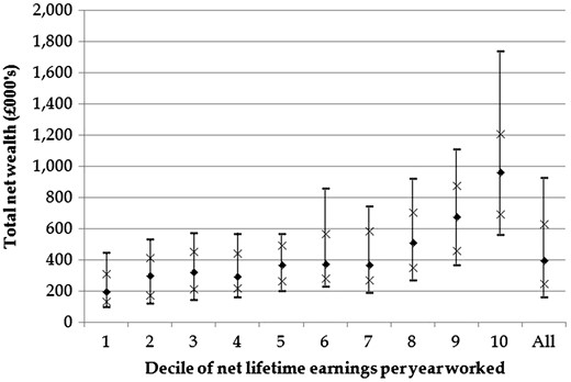
Tenth, 25th, 50th, 75th and 90th percentiles of total net wealth, by lifetime earnings decile (couples)

Notes: Sample size = 1,023; one observation per couple. The percentiles shown (from the bottom up) are the 10th, 25th, 50th, 75th, 90th percentiles. Total wealth is the sum of all financial, owner-occupied housing, state and private pension wealth, plus the value of any other physical assets (such as other property or business assets) held by the couple, less the value of any outstanding secured or unsecured debts. Non-housing wealth is total net wealth, less the (net of any outstanding mortgage) value of owner-occupied housing.

Source: ELSA data linked with NI records.

Open in new tab Download slide

Fig. 2

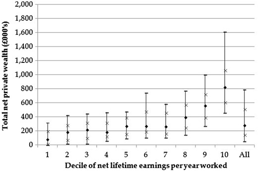
Tenth, 25th, 50th, 75th and 90th percentiles of total net private wealth, by lifetime earnings decile (couples)

Notes: Sample size = 1,023; one observation per couple. The percentiles shown (from the bottom up) are the 10th, 25th, 50th, 75th, 90th percentiles. Private wealth is the sum of all financial, owner-occupied housing and private pension wealth, plus the value of any other physical assets (such as other property or business assets) held by the couple, less the value of any outstanding secured or unsecured debts. Non-housing wealth is total net wealth, less the (net of any outstanding mortgage) value of owner-occupied housing.

Source: ELSA data linked with NI records.

Open in new tab Download slide

To test formally whether the differences we observe are statistically different, we run median regressions of the ratios of our different definitions of wealth to net lifetime earnings on quintiles of average earnings per year worked.¹⁷ Age dummies are included to control for the fact that our sample covers a reasonably wide age range and those individuals who are further into their retirement may already have started to decumulate some of the wealth.

The results are shown in Table 5. The first three columns show the results from regressions where the dependent variables are ratios of individual components of private wealth to lifetime earnings (respectively, private pension wealth, housing wealth, financial wealth). The dependent variable in the fourth column is the ratio of total private wealth to lifetime earnings. The definition of wealth used in the fifth column is state pension wealth and that in the sixth column is total wealth (the sum of private wealth and state pension wealth). The asterisks indicate whether the estimated coefficient differs statistically from the coefficient of the quintile below it (not whether there is a difference between it and the omitted category).

Table 5

Median regressions of the ratio of wealth to net lifetime earnings (using quintiles of lifetime earnings per year worked)

	(1)	(2)	(3)	(4)	(5)	(6)

	Private pension	Housing wealth	Financial wealth	Private wealth	State pension	Total wealth
Quintile of LE (rel. to lowest)
Quintile 2	2.738*	2.541**	0.620	3.728	–6.461***	–6.122**
	(1.523)	(1.061)	(0.666)	(2.564)	(0.570)	(2.401)
Quintile 3	4.307	3.132	2.136	7.806	–8.787***	–4.087
	(1.531)	(1.067)	(0.670)	(2.577)	(0.573)	(2.413)
Quintile 4	7.105*	3.170	2.498	11.199	–10.013**	–2.451
	(1.529)	(1.066)	(0.669)	(2.574)	(0.572)	(2.411)
Highest	13.420***	5.970***	5.351***	23.165***	–12.898***	6.338**
	(1.533)	(1.068)	(0.671)	(2.580)	(0.573)	(2.416)
Constant	12.645***	9.697***	1.000	29.060***	24.452***	56.834***
	(1.516)	(1.056)	(0.663)	(2.551)	(0.567)	(2.389)
Sample size	1023	1023	1023	1023	1023	1023

	(1)	(2)	(3)	(4)	(5)	(6)

	Private pension	Housing wealth	Financial wealth	Private wealth	State pension	Total wealth
Quintile of LE (rel. to lowest)
Quintile 2	2.738*	2.541**	0.620	3.728	–6.461***	–6.122**
	(1.523)	(1.061)	(0.666)	(2.564)	(0.570)	(2.401)
Quintile 3	4.307	3.132	2.136	7.806	–8.787***	–4.087
	(1.531)	(1.067)	(0.670)	(2.577)	(0.573)	(2.413)
Quintile 4	7.105*	3.170	2.498	11.199	–10.013**	–2.451
	(1.529)	(1.066)	(0.669)	(2.574)	(0.572)	(2.411)
Highest	13.420***	5.970***	5.351***	23.165***	–12.898***	6.338**
	(1.533)	(1.068)	(0.671)	(2.580)	(0.573)	(2.416)
Constant	12.645***	9.697***	1.000	29.060***	24.452***	56.834***
	(1.516)	(1.056)	(0.663)	(2.551)	(0.567)	(2.389)
Sample size	1023	1023	1023	1023	1023	1023

Notes: Standard errors in parentheses.

Sample: Couples, all lifetime earnings distribution.

Controls: We also have included age dummies in all specifications.

Asterisks indicate whether coefficients are statistically significantly different from the quintile below (rather than from zero): * $p < 0.1$ ⁠, ** $p < 0.05$ ⁠, *** $p < 0.01$ ⁠.

Table 5

Median regressions of the ratio of wealth to net lifetime earnings (using quintiles of lifetime earnings per year worked)

	(1)	(2)	(3)	(4)	(5)	(6)

	Private pension	Housing wealth	Financial wealth	Private wealth	State pension	Total wealth
Quintile of LE (rel. to lowest)
Quintile 2	2.738*	2.541**	0.620	3.728	–6.461***	–6.122**
	(1.523)	(1.061)	(0.666)	(2.564)	(0.570)	(2.401)
Quintile 3	4.307	3.132	2.136	7.806	–8.787***	–4.087
	(1.531)	(1.067)	(0.670)	(2.577)	(0.573)	(2.413)
Quintile 4	7.105*	3.170	2.498	11.199	–10.013**	–2.451
	(1.529)	(1.066)	(0.669)	(2.574)	(0.572)	(2.411)
Highest	13.420***	5.970***	5.351***	23.165***	–12.898***	6.338**
	(1.533)	(1.068)	(0.671)	(2.580)	(0.573)	(2.416)
Constant	12.645***	9.697***	1.000	29.060***	24.452***	56.834***
	(1.516)	(1.056)	(0.663)	(2.551)	(0.567)	(2.389)
Sample size	1023	1023	1023	1023	1023	1023

	(1)	(2)	(3)	(4)	(5)	(6)

	Private pension	Housing wealth	Financial wealth	Private wealth	State pension	Total wealth
Quintile of LE (rel. to lowest)
Quintile 2	2.738*	2.541**	0.620	3.728	–6.461***	–6.122**
	(1.523)	(1.061)	(0.666)	(2.564)	(0.570)	(2.401)
Quintile 3	4.307	3.132	2.136	7.806	–8.787***	–4.087
	(1.531)	(1.067)	(0.670)	(2.577)	(0.573)	(2.413)
Quintile 4	7.105*	3.170	2.498	11.199	–10.013**	–2.451
	(1.529)	(1.066)	(0.669)	(2.574)	(0.572)	(2.411)
Highest	13.420***	5.970***	5.351***	23.165***	–12.898***	6.338**
	(1.533)	(1.068)	(0.671)	(2.580)	(0.573)	(2.416)
Constant	12.645***	9.697***	1.000	29.060***	24.452***	56.834***
	(1.516)	(1.056)	(0.663)	(2.551)	(0.567)	(2.389)
Sample size	1023	1023	1023	1023	1023	1023

Notes: Standard errors in parentheses.

Sample: Couples, all lifetime earnings distribution.

Controls: We also have included age dummies in all specifications.

Asterisks indicate whether coefficients are statistically significantly different from the quintile below (rather than from zero): * $p < 0.1$ ⁠, ** $p < 0.05$ ⁠, *** $p < 0.01$ ⁠.

Private pension wealth (column 1) as a share of net lifetime earnings increases monotonically with quintiles of lifetime earnings, each coefficient being larger—and, with the exception of the third quintile, statistically significantly larger—than the one below. Turning to column 2, those in the middle three quintiles have a similar quantity of housing wealth (relative to their earnings), though this is more than that held by the bottom quintile, and less than that held by the top. Households in the bottom two quintiles hold very little financial wealth—with medians of 1% and 1.6%, respectively, of their lifetime earnings—compared to 6.4% for those in the top quintile.

Turning to all private wealth, the point estimates indicate that wealth as a share of net lifetime earnings is increasing at each quintile of the lifetime earnings distribution. While only those in the top quintile have statistically significantly more wealth than the quintile below them, both the third and fourth quintile have accumulated more wealth than those in the bottom quintile. With respect to private wealth, then, it is clear that the lifetime rich accumulate more.

The pattern is somewhat different when state pension wealth is included (column 6). The relationship between total wealth ratios to lifetime earnings and those earnings is non-monotonic. It declines between the first and second quintile—that is, couples at the bottom of the wealth distribution have higher wealth as a fraction of their lifetime earnings than those in the second quintile do. The differences between the results in columns 4 and 6 reflects the fact that the ratio of state pension wealth to lifetime earnings is negatively correlated with lifetime earnings per year worked, reflecting the fact that the state pension provides substantially more as a proportion of lifetime earnings to those with lower lifetime earnings (something that is clear from column 5). However, even on this broader measure of wealth, those in the top quintile of lifetime earnings have the highest ratios of wealth to lifetime earnings. The difference between the results in columns 4 and 6 is consistent with state pensions crowding out some private saving for those with low lifetime earnings (see Attanasio and Rohwedder [2003] for evidence of this in the UK).

Table 6 presents an alternative set of results—showing how the ratio of wealth to lifetime earnings differs across the distribution of total lifetime earnings (that is, rather than across the distribution of lifetime earnings per year worked, as is shown in Table 5). Looking at private wealth and its components, the conclusions from Table 6 are very similar to those described above. However, the relationship between total wealth and lifetime earnings is flat over the first four quintiles, with only those among the top 20% exhibiting statistically different savings behaviour.¹⁸

Table 6

Median regressions of the ratio of wealth to net lifetime earnings (using quintiles of actual lifetime earnings)

	(1)	(2)	(3)	(4)	(5)	(6)

	Private pension	Housing wealth	Financial wealth	Private wealth	State pension	Total wealth
Quintile of LE (rel. to lowest)
Quintile 2	3.769*	3.469***	1.726***	8.604***	–6.360***	0.352
	(1.680)	(1.080)	(0.616)	(2.529)	(0.529)	(2.688)
Quintile 3	4.230	4.270	2.580	10.909	–8.520***	–0.797
	(1.686)	(1.084)	(0.618)	(2.538)	(0.531)	(2.698)
Quintile 4	5.943	3.775	2.908	13.618	–10.156***	0.822
	(1.686)	(1.084)	(0.618)	(2.539)	(0.531)	(2.698)
Highest	12.876***	5.936**	5.507***	24.200***	–12.926***	7.038**
	(1.697)	(1.092)	(0.622)	(2.555)	(0.535)	(2.716)
Constant	12.722***	9.209***	0.908	26.231***	24.481***	54.500***
	(1.647)	(1.059)	(0.604)	(2.479)	(0.519)	(2.635)
Sample size	1023	1023	1023	1023	1023	1023

	(1)	(2)	(3)	(4)	(5)	(6)

	Private pension	Housing wealth	Financial wealth	Private wealth	State pension	Total wealth
Quintile of LE (rel. to lowest)
Quintile 2	3.769*	3.469***	1.726***	8.604***	–6.360***	0.352
	(1.680)	(1.080)	(0.616)	(2.529)	(0.529)	(2.688)
Quintile 3	4.230	4.270	2.580	10.909	–8.520***	–0.797
	(1.686)	(1.084)	(0.618)	(2.538)	(0.531)	(2.698)
Quintile 4	5.943	3.775	2.908	13.618	–10.156***	0.822
	(1.686)	(1.084)	(0.618)	(2.539)	(0.531)	(2.698)
Highest	12.876***	5.936**	5.507***	24.200***	–12.926***	7.038**
	(1.697)	(1.092)	(0.622)	(2.555)	(0.535)	(2.716)
Constant	12.722***	9.209***	0.908	26.231***	24.481***	54.500***
	(1.647)	(1.059)	(0.604)	(2.479)	(0.519)	(2.635)
Sample size	1023	1023	1023	1023	1023	1023

Notes: Standard errors in parentheses.

Sample: Couples, all lifetime earnings distribution.

Controls: We also have included age dummies in all specifications.

Asterisks indicate whether coefficients are statistically significantly different from the quintile below (rather than from zero): * $p < 0.1$ ⁠, ** $p < 0.05$ ⁠, *** $p < 0.01$ ⁠.

Table 6

Median regressions of the ratio of wealth to net lifetime earnings (using quintiles of actual lifetime earnings)

	(1)	(2)	(3)	(4)	(5)	(6)

	Private pension	Housing wealth	Financial wealth	Private wealth	State pension	Total wealth
Quintile of LE (rel. to lowest)
Quintile 2	3.769*	3.469***	1.726***	8.604***	–6.360***	0.352
	(1.680)	(1.080)	(0.616)	(2.529)	(0.529)	(2.688)
Quintile 3	4.230	4.270	2.580	10.909	–8.520***	–0.797
	(1.686)	(1.084)	(0.618)	(2.538)	(0.531)	(2.698)
Quintile 4	5.943	3.775	2.908	13.618	–10.156***	0.822
	(1.686)	(1.084)	(0.618)	(2.539)	(0.531)	(2.698)
Highest	12.876***	5.936**	5.507***	24.200***	–12.926***	7.038**
	(1.697)	(1.092)	(0.622)	(2.555)	(0.535)	(2.716)
Constant	12.722***	9.209***	0.908	26.231***	24.481***	54.500***
	(1.647)	(1.059)	(0.604)	(2.479)	(0.519)	(2.635)
Sample size	1023	1023	1023	1023	1023	1023

	(1)	(2)	(3)	(4)	(5)	(6)

	Private pension	Housing wealth	Financial wealth	Private wealth	State pension	Total wealth
Quintile of LE (rel. to lowest)
Quintile 2	3.769*	3.469***	1.726***	8.604***	–6.360***	0.352
	(1.680)	(1.080)	(0.616)	(2.529)	(0.529)	(2.688)
Quintile 3	4.230	4.270	2.580	10.909	–8.520***	–0.797
	(1.686)	(1.084)	(0.618)	(2.538)	(0.531)	(2.698)
Quintile 4	5.943	3.775	2.908	13.618	–10.156***	0.822
	(1.686)	(1.084)	(0.618)	(2.539)	(0.531)	(2.698)
Highest	12.876***	5.936**	5.507***	24.200***	–12.926***	7.038**
	(1.697)	(1.092)	(0.622)	(2.555)	(0.535)	(2.716)
Constant	12.722***	9.209***	0.908	26.231***	24.481***	54.500***
	(1.647)	(1.059)	(0.604)	(2.479)	(0.519)	(2.635)
Sample size	1023	1023	1023	1023	1023	1023

Notes: Standard errors in parentheses.

Sample: Couples, all lifetime earnings distribution.

Controls: We also have included age dummies in all specifications.

Asterisks indicate whether coefficients are statistically significantly different from the quintile below (rather than from zero): * $p < 0.1$ ⁠, ** $p < 0.05$ ⁠, *** $p < 0.01$ ⁠.

Given that our earnings measure relies, to an extent, on data that has been imputed, it is worth briefly discussing how measurement error could affect the interpretation of our results. Measurement error in our earnings measure will bias downwards the estimated relationship between lifetime earnings and wealth. This is for two reasons. First, lifetime earnings is both in the denominator of the dependent variable and is the basis for the regressors of interest (i.e. quintiles of earnings ability). Measurement error in lifetime earnings will generate a mechanical negative relationship between wealth to lifetime earnings ratios and quintiles of the lifetime earnings distribution and thus negatively bias the coefficient of interest. Second, reinforcing this is the bias coming from regression attenuation that occurs whenever a regressor is measured with error. These two features will bias downwards our estimate of the gradient of interest and makes our reported results conservative.

We conclude from these results that there is robust evidence using English data that those with the highest lifetime earnings—in the top 20% of lifetime earnings distribution—have the highest ratios of private wealth to earnings. In other words, there is evidence that in England the ‘rich save more’ (where the ‘rich’ are understood to be those in the top quintile).¹⁹ The relationship between lifetime earnings and wealth accumulation over the bottom 80% of the distribution depends on the measure of wealth analysed. While there is a positive relationship between accumulation of private wealth and earnings across the bottom four quintiles, those at the bottom accumulate more total wealth (include state pension wealth) that those in the middle.

Our results share some similarity with US studies. Hendricks (2007) finds that median private wealth (excluding social security wealth) accumulation rises with lifetime earnings. Additionally, our result that when public pension wealth is included, those at the bottom have more than those in the middle, has also be found by those using similar data in the US (Gustman and Steinmeier, 1999; Venti and Wise, 1998). That those in the top decile rich save more at the median has also been found by Venti and Wise (1998, see Their Table 1is on page 187, although the significance of the increase is not tested) though not Gustman and Steinmeier (1999, see their Table 6 is on Page 288 to 289).

In the remainder of this section we show results from regressions when other characteristics are included in the regression. Table 7 includes age dummies and quintiles of lifetime earnings per year worked, as well as the following additional covariates: (i) indicators of the education of each spouse (whether they have less than secondary education, have secondary education or have post-secondary education); (ii) indicators for whether each spouse self-reports that they are in either ‘poor’ or ‘fair’ health; (iii) indicators for having no children, having one or two children or having three or more children); (iv) indicators for life expectancy (their self-reported chance of living for at least another 10 or 15 years (depending on their current age); and (v) an indicator for having ‘high’ numerical ability.²⁰

Table 7

Median regressions of the ratio of wealth to net lifetime earnings

	(1)	(2)	(3)	(4)	(5)	(6)

	Private pension	Housing wealth	Financial wealth	Private wealth	State pension	Total wealth
Quintile 2	2.871	1.634	–0.147	2.697	–6.346***	–8.834***
	(1.275)	(1.184)	(0.656)	(2.336)	(0.564)	(2.505)
Quintile 3	4.600	2.221	0.683	3.874	–8.738***	–9.426
	(1.292)	(1.200)	(0.665)	(2.368)	(0.572)	(2.539)
Quintile 4	5.128	1.375	1.123	5.716	–9.630	–9.212
	(1.306)	(1.212)	(0.672)	(2.393)	(0.578)	(2.567)
Highest	7.219	0.978	1.312	7.799	–12.514***	–9.456
	(1.404)	(1.303)	(0.722)	(2.572)	(0.621)	(2.758)
Husband’s education (rel. to less than high school)
Secondary education	3.806***	3.191***	2.658***	8.809***	0.323	9.033***
	(1.025)	(0.952)	(0.527)	(1.879)	(0.454)	(2.015)
Higher education	5.536***	3.799**	2.582***	12.123***	–0.155	10.342***
	(1.440)	(1.337)	(0.741)	(2.639)	(0.638)	(2.830)
Wife’s education (rel. to less than high school)
Sec. educ.	4.298***	1.941*	1.352**	8.276***	–0.591	7.524***
	(0.957)	(0.888)	(0.492)	(1.753)	(0.424)	(1.881)
Higher education	7.510***	1.260	1.964*	13.121***	–0.334	13.871***
	(1.544)	(1.433)	(0.794)	(2.828)	(0.684)	(3.034)
Husband in fair/	–1.455	–2.920**	–0.814	–3.756*	0.259	–0.706
poor health	(0.962)	(0.893)	(0.495)	(1.763)	(0.426)	(1.891)
Wife in	–0.420	–1.543	–0.739	–3.835*	0.302	–4.947*
fair/poor health	(1.007)	(0.934)	(0.518)	(1.844)	(0.446)	(1.978)
No children	–1.843	–0.365	0.564	–2.449	0.126	1.460
	(1.618)	(1.501)	(0.832)	(2.963)	(0.716)	(3.178)
3+ children	–0.909	–0.880	–0.568	–1.495	–0.075	–1.211
	(0.860)	(0.798)	(0.442)	(1.576)	(0.381)	(1.690)
Male life expectancy	0.103	0.777	–0.306	1.489	0.280	1.854
	(0.921)	(0.855)	(0.474)	(1.688)	(0.408)	(1.811)
Female life expectancy	0.943	1.369	0.736	3.570*	–0.229	2.161
	(0.849)	(0.788)	(0.436)	(1.554)	(0.376)	(1.667)
High number	2.599**	2.614**	1.006*	8.333***	–0.418	6.911***
	(0.903)	(0.839)	(0.465)	(1.655)	(0.400)	(1.775)
Sample size	1023	1023	1023	1023	1023	1023

	(1)	(2)	(3)	(4)	(5)	(6)

	Private pension	Housing wealth	Financial wealth	Private wealth	State pension	Total wealth
Quintile 2	2.871	1.634	–0.147	2.697	–6.346***	–8.834***
	(1.275)	(1.184)	(0.656)	(2.336)	(0.564)	(2.505)
Quintile 3	4.600	2.221	0.683	3.874	–8.738***	–9.426
	(1.292)	(1.200)	(0.665)	(2.368)	(0.572)	(2.539)
Quintile 4	5.128	1.375	1.123	5.716	–9.630	–9.212
	(1.306)	(1.212)	(0.672)	(2.393)	(0.578)	(2.567)
Highest	7.219	0.978	1.312	7.799	–12.514***	–9.456
	(1.404)	(1.303)	(0.722)	(2.572)	(0.621)	(2.758)
Husband’s education (rel. to less than high school)
Secondary education	3.806***	3.191***	2.658***	8.809***	0.323	9.033***
	(1.025)	(0.952)	(0.527)	(1.879)	(0.454)	(2.015)
Higher education	5.536***	3.799**	2.582***	12.123***	–0.155	10.342***
	(1.440)	(1.337)	(0.741)	(2.639)	(0.638)	(2.830)
Wife’s education (rel. to less than high school)
Sec. educ.	4.298***	1.941*	1.352**	8.276***	–0.591	7.524***
	(0.957)	(0.888)	(0.492)	(1.753)	(0.424)	(1.881)
Higher education	7.510***	1.260	1.964*	13.121***	–0.334	13.871***
	(1.544)	(1.433)	(0.794)	(2.828)	(0.684)	(3.034)
Husband in fair/	–1.455	–2.920**	–0.814	–3.756*	0.259	–0.706
poor health	(0.962)	(0.893)	(0.495)	(1.763)	(0.426)	(1.891)
Wife in	–0.420	–1.543	–0.739	–3.835*	0.302	–4.947*
fair/poor health	(1.007)	(0.934)	(0.518)	(1.844)	(0.446)	(1.978)
No children	–1.843	–0.365	0.564	–2.449	0.126	1.460
	(1.618)	(1.501)	(0.832)	(2.963)	(0.716)	(3.178)
3+ children	–0.909	–0.880	–0.568	–1.495	–0.075	–1.211
	(0.860)	(0.798)	(0.442)	(1.576)	(0.381)	(1.690)
Male life expectancy	0.103	0.777	–0.306	1.489	0.280	1.854
	(0.921)	(0.855)	(0.474)	(1.688)	(0.408)	(1.811)
Female life expectancy	0.943	1.369	0.736	3.570*	–0.229	2.161
	(0.849)	(0.788)	(0.436)	(1.554)	(0.376)	(1.667)
High number	2.599**	2.614**	1.006*	8.333***	–0.418	6.911***
	(0.903)	(0.839)	(0.465)	(1.655)	(0.400)	(1.775)
Sample size	1023	1023	1023	1023	1023	1023

Notes: Standard errors in parentheses.

Sample: Couples, all lifetime earnings distribution.

Controls: Dummies for age and decile of lifetime earnings per year worked included in all specifications. ‘Life expectancy’ is an indicator of whether the man/woman in the couple reported at least a 75% chance of surviving for another 10–15 years.

Asterisks on quintile dummies indicate whether coefficients are statistically significantly different from the quintile below (rather than from zero). Asterisks on other coefficients show statistical difference from zero: * $p < 0.1$ ⁠, ** $p < 0.05$ ⁠, *** $p < 0.01$ ⁠.

Table 7

Median regressions of the ratio of wealth to net lifetime earnings

	(1)	(2)	(3)	(4)	(5)	(6)

	Private pension	Housing wealth	Financial wealth	Private wealth	State pension	Total wealth
Quintile 2	2.871	1.634	–0.147	2.697	–6.346***	–8.834***
	(1.275)	(1.184)	(0.656)	(2.336)	(0.564)	(2.505)
Quintile 3	4.600	2.221	0.683	3.874	–8.738***	–9.426
	(1.292)	(1.200)	(0.665)	(2.368)	(0.572)	(2.539)
Quintile 4	5.128	1.375	1.123	5.716	–9.630	–9.212
	(1.306)	(1.212)	(0.672)	(2.393)	(0.578)	(2.567)
Highest	7.219	0.978	1.312	7.799	–12.514***	–9.456
	(1.404)	(1.303)	(0.722)	(2.572)	(0.621)	(2.758)
Husband’s education (rel. to less than high school)
Secondary education	3.806***	3.191***	2.658***	8.809***	0.323	9.033***
	(1.025)	(0.952)	(0.527)	(1.879)	(0.454)	(2.015)
Higher education	5.536***	3.799**	2.582***	12.123***	–0.155	10.342***
	(1.440)	(1.337)	(0.741)	(2.639)	(0.638)	(2.830)
Wife’s education (rel. to less than high school)
Sec. educ.	4.298***	1.941*	1.352**	8.276***	–0.591	7.524***
	(0.957)	(0.888)	(0.492)	(1.753)	(0.424)	(1.881)
Higher education	7.510***	1.260	1.964*	13.121***	–0.334	13.871***
	(1.544)	(1.433)	(0.794)	(2.828)	(0.684)	(3.034)
Husband in fair/	–1.455	–2.920**	–0.814	–3.756*	0.259	–0.706
poor health	(0.962)	(0.893)	(0.495)	(1.763)	(0.426)	(1.891)
Wife in	–0.420	–1.543	–0.739	–3.835*	0.302	–4.947*
fair/poor health	(1.007)	(0.934)	(0.518)	(1.844)	(0.446)	(1.978)
No children	–1.843	–0.365	0.564	–2.449	0.126	1.460
	(1.618)	(1.501)	(0.832)	(2.963)	(0.716)	(3.178)
3+ children	–0.909	–0.880	–0.568	–1.495	–0.075	–1.211
	(0.860)	(0.798)	(0.442)	(1.576)	(0.381)	(1.690)
Male life expectancy	0.103	0.777	–0.306	1.489	0.280	1.854
	(0.921)	(0.855)	(0.474)	(1.688)	(0.408)	(1.811)
Female life expectancy	0.943	1.369	0.736	3.570*	–0.229	2.161
	(0.849)	(0.788)	(0.436)	(1.554)	(0.376)	(1.667)
High number	2.599**	2.614**	1.006*	8.333***	–0.418	6.911***
	(0.903)	(0.839)	(0.465)	(1.655)	(0.400)	(1.775)
Sample size	1023	1023	1023	1023	1023	1023

	(1)	(2)	(3)	(4)	(5)	(6)

	Private pension	Housing wealth	Financial wealth	Private wealth	State pension	Total wealth
Quintile 2	2.871	1.634	–0.147	2.697	–6.346***	–8.834***
	(1.275)	(1.184)	(0.656)	(2.336)	(0.564)	(2.505)
Quintile 3	4.600	2.221	0.683	3.874	–8.738***	–9.426
	(1.292)	(1.200)	(0.665)	(2.368)	(0.572)	(2.539)
Quintile 4	5.128	1.375	1.123	5.716	–9.630	–9.212
	(1.306)	(1.212)	(0.672)	(2.393)	(0.578)	(2.567)
Highest	7.219	0.978	1.312	7.799	–12.514***	–9.456
	(1.404)	(1.303)	(0.722)	(2.572)	(0.621)	(2.758)
Husband’s education (rel. to less than high school)
Secondary education	3.806***	3.191***	2.658***	8.809***	0.323	9.033***
	(1.025)	(0.952)	(0.527)	(1.879)	(0.454)	(2.015)
Higher education	5.536***	3.799**	2.582***	12.123***	–0.155	10.342***
	(1.440)	(1.337)	(0.741)	(2.639)	(0.638)	(2.830)
Wife’s education (rel. to less than high school)
Sec. educ.	4.298***	1.941*	1.352**	8.276***	–0.591	7.524***
	(0.957)	(0.888)	(0.492)	(1.753)	(0.424)	(1.881)
Higher education	7.510***	1.260	1.964*	13.121***	–0.334	13.871***
	(1.544)	(1.433)	(0.794)	(2.828)	(0.684)	(3.034)
Husband in fair/	–1.455	–2.920**	–0.814	–3.756*	0.259	–0.706
poor health	(0.962)	(0.893)	(0.495)	(1.763)	(0.426)	(1.891)
Wife in	–0.420	–1.543	–0.739	–3.835*	0.302	–4.947*
fair/poor health	(1.007)	(0.934)	(0.518)	(1.844)	(0.446)	(1.978)
No children	–1.843	–0.365	0.564	–2.449	0.126	1.460
	(1.618)	(1.501)	(0.832)	(2.963)	(0.716)	(3.178)
3+ children	–0.909	–0.880	–0.568	–1.495	–0.075	–1.211
	(0.860)	(0.798)	(0.442)	(1.576)	(0.381)	(1.690)
Male life expectancy	0.103	0.777	–0.306	1.489	0.280	1.854
	(0.921)	(0.855)	(0.474)	(1.688)	(0.408)	(1.811)
Female life expectancy	0.943	1.369	0.736	3.570*	–0.229	2.161
	(0.849)	(0.788)	(0.436)	(1.554)	(0.376)	(1.667)
High number	2.599**	2.614**	1.006*	8.333***	–0.418	6.911***
	(0.903)	(0.839)	(0.465)	(1.655)	(0.400)	(1.775)
Sample size	1023	1023	1023	1023	1023	1023

Notes: Standard errors in parentheses.

Sample: Couples, all lifetime earnings distribution.

A number of points are worth stressing. First, in all specifications, measures of further education have significant positive coefficients. That is, we find that higher levels of education are associated with higher levels of wealth, even after controlling for lifetime earnings. This could be driven by a tendency for those with low discount rates both to invest more in education and to save more or could be indicative of a causal effect of education on saving behaviour.

Second, the indicator of having ‘high’ numerical ability has a large, positive and significant coefficient. Even controlling for education and lifetime earnings, individuals who are able to compute compound interest rates seem to exhibit higher wealth to earnings ratios than less numerate individuals. This measure of cognitive ability could act as proxy for low time preference and/or an ability to earn higher returns on savings.

The coefficients on the measures of poor health, expectations of survival and having children are not statistically significantly different from zero in most cases. However, the signs on some of these coefficients are perhaps interesting. Those who expect a higher probability of surviving for another 10 to 15 years have higher wealth to earnings ratios. This is consistent with the fact that they should expect to have a greater fraction of their lives left to fund. Those who are in poor health tend to have lower wealth to earnings ratios than those in better health. This is consistent with them having incurred health-related expenses earlier in life.

Turning to the coefficients on lifetime earnings quintile, the qualitative findings regarding private wealth and its components are the same as those found in Table 5. While in all cases the coefficients on quintiles 4 and 5 are statistically different from that on quintile 1 (the omitted category), we are not able to reject that adjoining quintiles have statistically different results. The main difference with respect to the results in Table 5 are found for total wealth including state pensions. As in the results in Table 5 those in the bottom earnings quintile accumulate more wealth relative to earnings than those in the next quintile. However, we no longer find a positive association with being in the top 20% of the lifetime earnings distribution and accumulating the most wealth. The extra wealth that we observe for those in the top 20% in the raw data is explained by a combination of their higher education and greater numerical ability; those with the most lifetime earnings conditional on these actually accumulate less than those with the least.

These additional results should not be considered tests of the underlying mechanism are that generate our primary results (the gradients of different measures of wealth accumulated with respect to lifetime earnings). The positive relationship between education (which explains at least some of our primary results), for example, could represent a causal effect of greater education or it could represent an underlying propensity to save (driven, perhaps by greater patience) among those who select into greater education. Further research will, hopefully, shed greater light on these mechanisms.

5. Conclusion

Using newly available and previously unexploited English administrative data on employment since 1948 and earnings since 1975 linked with ELSA, this paper looks at the relationship between wealth to earnings ratios and various measures of lifetime earnings. We have shown that there is a robust positive relationship between the ratio of private wealth to lifetime earnings (that is wealth excluding public pension wealth) and earnings ability. The effect is strongest among those in the top quintile of the lifetime earnings distribution—they have substantially greater wealth relative to their earnings than those in the bottom 80% of the distribution.

While there is a monotonic relationship between saving in private forms and lifetime earnings, once the measure of wealth is defined to include state pension wealth, the relationship becomes non-monotonic. Those in the top 20% still accumulate more wealth than those in the rest of the distribution, but those in the bottom quintile exhibits higher levels of this broader wealth measure than those in the middle of the distribution. The fact that the UK state pension system gives the highest replacement rates to those workers who have earned the least more then offsets the lesser private saving of those in the bottom of the lifetime earnings distribution relative to those in the middle. Those in the middle of the lifetime earnings distribution have the lowest total wealth to earnings ratios. As a proportion of their lifetime earnings, these households have lower state pension wealth than the poorest, and have accumulated less private wealth than the richest.

A caveat to our results is that we make no claim that our results are generalizable to the behaviour of extremely wealthy households. Our data do not oversample the very wealthy and, therefore, we cannot say much about the behaviour of the ‘top 1%’, who have been of such interest to the general public and researchers alike (Alvaredo et al., 2013, 2016). The saving behaviour of this group is an interesting topic for future research.

Supplementary material

Supplementary material (the Appendix) is available online at the OUP website. The ELSA data were supplied by the UK Data Archive and the copyright is held jointly by the Institute for Fiscal Studies, the National Centre for Social Research and University College London. Access to ELSA respondents’ National Insurance records was kindly granted by HM Revenue and Customs and the ELSA Linked Data Advisory Committee (ELDAC). The Stata do files to replicate the results have been made available on the website.

Funding

This work was supported by the IFS Retirement Saving Consortium; the Economic and Social Research Council (‘Centre for the Microeconomic Analysis of Public Policy’ [grant reference: ES/M010147/1] and Secondary Data Analysis Initiative Grant ‘Adequacy and Optimality of Retirement Provision: Household Behaviour and the Design of Pensions’ [grant reference: ES/N011872/1] to COD); and the European Research Council [grant reference: ERC-2010-AdG Grant Agreement Number 269440 – WSCWTBDS] to AB and COD. The English Longitudinal Study of Ageing (ELSA) is funded by the National Institute on Aging and a consortium of UK government departments.

Footnotes

The result that saving and accumulated wealth are proportional to lifetime earnings does, however, continue to hold if uncertainty of some very specific types is introduced (see Bar-Ilan, 1995).

The results that we will present are very similar when an interest rate (another obvious candidate) is used to calculate the present value.

Additionally if years in work is mismeasured this division could increase the effect that measurement error has on our results.

For a history of state pensions in the UK see Bozio et al. (2010b).

As discussed later, neither of these groups are included in our sample.

For a more detailed discussion of the extent to which the linked sample is representative of the full sample see Bozio et al. (2010a).

Unfortunately, only the first wave of ELSA has been linked to the NI records.

Accrued state pension income is calculated using the administrative data. A household’s state pension wealth is the present discounted value of their accrued stream of income. Details on how it is calculated are given in Section 3.1 of Crawford et al. (2014). For further details on the calculation of private pension wealth in ELSA see Banks et al. (2005).

The proportion of our sample who have censored earnings in a particular year varies between 8.6% and 15.9%. Twenty per cent of our sample have earnings censored in one year between 1975 and 1996.

The fixed-effect Tobit, when the length of the panel is fixed, is known to yield inconsistent results due to the incidental parameters problem. However, Greene (2004) investigates, using Monte Carlo methods, its properties and finds that parameters of the fixed effects Tobit model are little affected by this problem even with panel of lengths substantially shorter than our panel (which has length 29). Further, an examination of selected quantiles of earnings through time using the censored and imputed data prior to 1997 and the uncensored data from 1997 onwards shows only a very small discontinuity in 1997.

Net earnings are calculated using the UK’s NI and income tax schedules in each year from 1948 to 2002. Details can be found in Appendix B.

While our measure of wealth includes pension wealth that is due to employer contributions, our measure of lifetime earnings will not include these flows. If these contributions increase (decrease) in proportionate terms with lifetime earnings, our results will be somewhat biased in favour (against) a finding of increased saving by the rich.

The only component of wealth not shown here is physical wealth (vehicles, jewellery, etc.), which accounts for 5% of average wealth.

The public pension system that applied to our cohort of interest is briefly described in Appendix C—a more detailed treatment is give in Bozio et al. (2010b).

Gross earnings are adjusted for taxes paid, but not for benefits received. Our data are not sufficient to go from this measure of earnings net of taxes to net income—inclusive of all state transfers. The analysis will therefore under-represent the actual degree of redistribution produced by the tax and benefit system.

These are obtained by calculating the ratio of wealth to lifetime earnings for each couple in the sample and then taking the median. This median ratio differs from the ratio of the medians which involves taking the ratio of median wealth to median lifetime earnings for each decile. The latter approach yields almost identical results.

Specifically, we divide each partner’s earnings by their number of years in paid work and sum these annual earnings between the ages of 16 and 64.

The differences between the results in these two tables can be understood by considering the implications of the different definition of lifetime earnings used to construct the quintiles. Those in the bottom decile in regressions reported in Table 5 have lower earnings per year but work more years than those in the bottom decile in Table 6. The state pension system provides greater payments to the former group who work for more years.

The results are robust to restricting the sample to only those who have been married once (for those who were previously married, we may be missing earnings data from former spouses) and to restricting it to those aged between 60 and 65 (who are nearer retirement).

This variable indicates respondents are able to perform correctly a calculation that involves an understanding of compound interest, see Banks et al. (2010) for more detail on how it is constructed.

Acknowledgements

We thank James Banks, Richard Blundell, Thomas F. Crossley, Peter Diamond, Richard Disney, Michael Hurd, Tullio Jappelli, Paul Johnson, Guy Laroque, David Wise, Stephen Zeldes, two anonymous referees as well as seminar participants at the NBER Summer Institute for useful comments. Responsibility for interpretation of the data, as well as for any errors, is the authors’ alone.

References

Alan

Atalay

Crossley

T.F.

(

2015

)

Do the rich save more? Evidence from Canada

Review of Income and Wealth

739

–

Month:	Total Views:
May 2017	51
June 2017	26
July 2017	10
August 2017	11
September 2017	7
October 2017	80
November 2017	35
December 2017	57
January 2018	43
February 2018	65
March 2018	65
April 2018	65
May 2018	143
June 2018	74
July 2018	37
August 2018	43
September 2018	52
October 2018	40
November 2018	58
December 2018	40
January 2019	46
February 2019	48
March 2019	47
April 2019	46
May 2019	49
June 2019	29
July 2019	32
August 2019	43
September 2019	69
October 2019	61
November 2019	51
December 2019	38
January 2020	26
February 2020	63
March 2020	73
April 2020	31
May 2020	34
June 2020	68
July 2020	54
August 2020	30

Article Contents

Do the rich save more? Evidence from linked survey and administrative data

Abstract

1. Introduction

2. Theoretical background

2.1 A simple life cycle model

2.2 Departures from this model

3. Methodology and data

3.1 Empirical approach

3.2 Data

3.3 Descriptive statistics

4. Results

5. Conclusion

Supplementary material

Funding

Footnotes

Acknowledgements

References

Supplementary data

Citations

Views

Altmetric

Email alerts

Citing articles via

Latest

Most Read

Most Cited

This Feature Is Available To Subscribers Only