


Abstract
The paper considers the austerity measures introduced in the wake of the financial and economic crisis in the late 2000s in relation to their distributional impact across households and potential effects on aggregate demand. We determine the size, composition and effects of fiscal consolidation using a ‘bottom-up’ measurement strategy and find notable cross-country variation. We show that while richer households tend to bear a greater burden in most countries, combined cuts in public wages and transfers are more likely to affect liquidity-constrained households and thereby aggregate demand, casting doubts on the presumed effectiveness of such measures for macro-economic recovery. This suggests that in order to reach robust policy conclusions it is important to consider the distributional patterns of detailed policy measures.
1. Introduction
Following the financial and economic crisis which started in the late 2000s, governments introduced extensive fiscal consolidation measures to address budget deficits. The way in which fiscal consolidation is achieved and the cost of the crisis is distributed has implications for the prospects for macro-economic recovery and financial stability, as well as for the political acceptability of pathways in this direction.
Several studies have suggested that fiscal adjustments based on spending cuts, including both cuts in government services and public transfers to households, are more effective in reducing public debt and less harmful to economic growth than fiscal adjustments based on tax increases (e.g. Alesina and Perotti, 1995, 1997; McDermott and Wescott, 1996; Alesina and Ardagna 1998, 2010, 2013; von Hagen and Strauch, 2001; IMF, 2010; Guajardo et al., 2011; Alesina et al., 2012).1 Nevertheless, recent studies based on structural macro models shed some light on the fact that cuts in (unproductive) government spending are associated with long-run benefits but they can have short-run adjustment costs and pronounced distributional effects. In particular, some studies highlight the potentially detrimental effects of cuts in public transfers that are borne by liquidity-constrained households (Coenen et al., 2008, 2012; Forni et al., 2010; Clinton et al., 2011).
Such studies, however, tend to take a macro-economic perspective and overlook how measures affect the whole distribution of household incomes, which could be a critical element for determining the impact of policies on aggregate demand. Indeed, it is increasingly recognized in the economic literature that it is important to consider the heterogeneity of agents in order to avoid aggregation bias (e.g. Blundell and Stoker, 2005). For example, one might expect that cuts in non-contributory public transfers place a greater burden on the lower part of household income distribution, while tax increases require relatively bigger contributions from richer households who have a lower marginal propensity to consume, resulting in a smaller effect on aggregate demand. As recognized in Coenen et al. (2008), it is important to stress that the distributional effects depend on the overall design of the tax-benefit systems and also vary notably among specific benefit and tax instruments, pointing to the need to consider even more disaggregated categories.
Nevertheless, the distributional consequences of fiscal consolidation have been recognized to be of potential importance (Coenen et al., 2008). For example, Perotti (1996, p. 108) already stated: ‘The crucial question, however, remains the impact of fiscal consolidations on the distribution of disposable income. On this, there is very little information, because very rarely does the timing of income-distribution surveys allow an analysis of its evolution before and after a fiscal consolidation …’. His claim is still valid after almost 20 years in spite of the generally wider availability of microdata than in the 1990s. Although, more recently, there has been a notable increase in concern about the distributional consequences of the economic crisis, fiscal stimulus packages and fiscal consolidation measures, an assessment of the effect on the income distribution is still lacking not least because of data availability and difficulties in linking various budget items to specific household characteristics and in building a proper counterfactual scenario (Joumard et al., 2012).
The aim of this paper is to fill a gap in the fiscal consolidation literature regarding distributional effects, taking a cross-country perspective to give a stronger base for generalizing the results. First, considering the actual design of the fiscal consolidation measures, we provide evidence on the distributional impact of the austerity measures implemented in EU countries up to 2012. Second, we explore to what extent the design of the measures is associated with the potential impact on the consumption reactions of individuals and households facing the burden of the austerity measures. To the best of our knowledge we are the first to quantify the size, the distributive effects and the incidence on liquidity-constrained households of the fiscal consolidation measures actually faced by the household sector. This evidence does not only matter in its own right but can in principle offer valuable insights into the macro-economic performance of fiscal adjustments, complementing the flourishing macro-economic literature. Moreover, our paper provides a methodological approach for estimating (ex ante) the impact of fiscal consolidation measures on household disposable income that can be fed into macro-models. For example, our approach could potentially offer micro-based estimates to enrich the calibration of the structural parameters of the fiscal structure of macro models (e.g. Coenen et al., 2012), allowing for the definition of scenarios which track the policy rules implemented in reality rather than stylized scenarios which are often not plausible specifications for a given country (e.g. Clinton et al., 2011).
We make use of microsimulation techniques, which allow us to simulate tax-benefit policy changes in detail and estimate their effect on disposable income for each household in a nationally representative sample, with the help of relevant counterfactual scenarios. Aggregating the impact across all households yields a measure of total fiscal consolidation in the household sector, providing an alternative, ‘bottom-up’ measurement strategy to the usual approaches in the macro-economic literature. Specifically, we employ EUROMOD, the only EU-wide tax-benefit model, and concentrate our analysis on the Southern European countries (Greece, Italy, Portugal and Spain), the Baltic countries (Estonia, Latvia and Lithuania) and Romania which experienced the largest budget deficits and/or reductions in economic output during the crisis. These countries are also among those developed economies which have implemented or announced the largest fiscal consolidation, ranging between 6% and 18% of GDP (OECD, 2012; Sutherland et al., 2012).
Our paper has common elements with the strand of fiscal consolidation literature that uses a narrative approach to identify discretionary changes in fiscal policy (e.g. IMF, 2010; Romer and Romer, 2010) rather than statistical methods (e.g. Alesina and Perotti, 1995; Alesina and Ardagna, 1998; Blanchard and Perotti, 2002). However, unlike other studies relying on a narrative approach, we exploit the microsimulation model to derive our own estimates of fiscal consolidation measures, and their incidence across the income distribution, in a common framework rather than relying on official assessments by governments. An additional advantage of the microsimulation method in this context is that it allows for a focus on the design of the consolidation measures and an assessment of policy changes in great detail as we can consider each individual policy instrument separately as well as in combination.
Overall, our study is the first attempt to model the (short-term) effect of fiscal consolidation measures on the full income distribution. Previous studies focusing on the distributional impact of fiscal consolidation measures (often identified based on statistical methods) take a time-series perspective using episodes of fiscal consolidation for a sample of countries over a long period, to estimate the impact on aggregate inequality or poverty and to analyse the determinants of cross-country variations in income inequality (Ball et al., 2013; Woo et al., 2013; Agnello and Sousa, 2014). In contrast, we have estimated the distributional effects of a specific (and important) episode for a number of countries, identifying and modelling fiscal consolidation policies in great detail.
The degree of deficit reduction that the countries which are included in our analysis set out to achieve, influenced by the Stability and Growth Pact rules, naturally varied, and so did the policy mix chosen to achieve it. Our analysis addresses the question of how changes to direct and indirect (personal) taxes, cash benefits and public sector pay – which have a direct impact on household (cash) resources – affected different income groups. We focus on these instruments as they provide governments with better control on distributional outcomes and offer more explicit choices, while macro-economic and labour market policies – and even cuts in public services – are blunt instruments in terms of their distributional effects.
The extent to which a decrease in disposable income due to fiscal consolidation measures reduces household spending on goods and services provides a link between our micro-based approach and the macro literature on fiscal consolidation. We exploit the variation in income among households and link such a change to the potential reduction in their consumption, depending on the liquidity constraints they face (Auerbach and Feenberg, 2000; Coenen et al., 2012). Our approach shows the importance of the interactions between the design of fiscal consolidation measures and the income distribution; these matter on their own but also for the prospects for macro-economic recovery.
We find notable variation in the size, composition and first order effects of fiscal consolidation. Overall, richer households tend to bear a greater burden in most countries, though this differs a lot between types of tax-benefit instruments. Such heterogeneity tends to be less visible when measures are grouped as cuts of public transfers and tax increases, a dichotomy which is typically used in the fiscal adjustment literature. Moreover, our finding that combined cuts in public wages and transfers are more likely to affect liquidity-constrained households casts doubts about such measures being less detrimental for aggregate demand than increases in taxes. This suggests that it is not the type of policy instrument per se which matters but how it affects different parts of income distributions, hence our emphasis on the need to consider more disaggregated evidence to reach robust policy conclusions.
The remainder of the paper is structured as follows. Section 2 discusses methodology and summarizes the fiscal consolidation measures taken in each country and the scope of our analysis. Section 3 presents an analysis of the composition and distributional effects of the measures in the eight countries considered and shows how the different policy mixes each have their own distributional implications as well as certain common features. Section 4, provides micro-based insights to the macro-economic effects of austerity policies, by combining the design aspects of the austerity measures with their potential impact on aggregate demand, taking into account the liquidity constraints faced by households in the crisis period. The final section concludes by summarizing our policy relevant findings.
2. Methodology
2.1 Fiscal microsimulation
We focus on policy measures which directly impact household budgets and household aggregate demand, and which were introduced explicitly in order to cut the public deficit or stem its growth. These policy changes were not only many but also typically applied across the board, affecting large parts of population to some extent or another, and therefore provided no natural control groups for estimating causal effects on household incomes and demand. We therefore make use of fiscal microsimulation techniques (Bourguignon and Spadaro, 2006; Figari et al., 2015) to define and construct a counterfactual scenario: what would have happened in the absence of the fiscal consolidation measures.
In essence, fiscal or ‘tax-benefit’ microsimulation modelling applies detailed tax-benefit policy rules to a representative sample of households, using survey or register information on household characteristics and market income as input. It enables the derivation of disposable income for each household as well as the overall distribution under existing tax-benefit systems and, more importantly, the effect of tax-benefit policy changes on the household income distribution. In doing so, the heterogeneity in household budget constraints due to the interactions between the detailed tax-benefit rules and personal and household characteristics is fully taken into account. The focus on the entire distribution of changes in the target variable (rather than change for an average person or in the mean value alone) is one of the key distinctions from regression techniques or macro models. The first-order impact of tax-benefit policy changes on household incomes, i.e. the mechanical effect, is estimated without imposing any behavioural relationships and is strictly atheoretical. Static calculations also represent an important element of behavioural models, where these are combined with behavioural assumptions or a (detailed) choice mechanism.
We depart from purely arithmetic calculations and capture not only the first-order effects but also the extent to which these translate into changes in aggregate demand given that households have different capacities to absorb income shocks (due to liquidity constraints) and were affected by different types of policy measures (benefit cuts vs tax increases). Our micro-based approach is novel in the literature on fiscal consolidation, which is typically based on macro-economic evidence alone. Microsimulation modelling has already been used to consider the role of tax-benefit policies in stabilizing aggregate household demand to (hypothetical) income or unemployment shocks in the presence of liquidity constraints (Dolls et al., 2012), while our study is the first to consider the effect of actual policy changes in this context. Our analysis is partial as it does not attempt to cover wider general equilibrium or dynamic effects. We focus on household demand and liquidity constraints, leaving aside potential labour supply changes (as these are likely to be of second order in terms of magnitude) as well as other sectors in the economy (businesses, government spending on public goods and services).
2.2 The counterfactual
We identify and simulate changes in national legislation regarding individual tax and benefit instruments introduced for austerity reasons since the beginning of the economic downturn in 2008. We evaluate the effect of such austerity measures in 2012, the reference point in time of our simulations, at which point fiscal adjustments were at their maximum in most of the countries considered. The starting point from which measures were introduced is different across countries depending on many factors, including the timing of the national macro-economic and budgetary reactions to the financial crisis in order to respect the formal fiscal rules imposed by the Stability and Growth Pact. Among the countries included in the analysis, the Baltic countries (Estonia, Latvia and Lithuania) and Portugal started introducing fiscal consolidation measures in 2009 and followed with further measures in 2010 to 2012. Other countries (Greece, Spain and Romania) started fiscal consolidation in 2010 and Italy introduced its first measures in 2011.
Our aim is to distinguish between changes that were part of a ‘business as usual’ scenario and those introduced for austerity reasons. While the latter mostly involved tax increases and cuts in social benefits and public sector pay, such policy changes also included increases in some benefits or reductions in taxes for certain groups to compensate or alleviate the impact of other measures. On the other hand, we do not consider the expiry of fiscal stimulus measures as part of the fiscal consolidation package if those were intended to be temporary from the beginning. Overall, we follow the spirit of other studies relying on historic sources (e.g. IMF, 2010; Romer and Romer, 2010; Devries et al., 2011). We have chosen to interpret the ‘absence of the fiscal consolidation measures’, i.e. our counterfactual scenario, as the continuation of pre-fiscal consolidation policies, indexed according to standard practice and official assumption, or law. Such indexation of monetary values of tax-benefit policies is not the same across countries under consideration. Apart from public pensions, most of the countries do not regularly index fiscal policies and instead change these occasionally on an ad hoc basis. The only countries not applying any indexation are Greece and Lithuania.
To estimate the effect of policies we apply both the actual 2012 tax-benefit policies and the (indexed) pre-fiscal consolidation policies to the same households, keeping their characteristics (including market incomes) constant. This allows us to isolate the policy effect from changes in other dimensions (e.g. demographics or labour market outcomes). It is important to note that the estimation of policy effects is, however, conditional on market income and household characteristics in a particular moment in time, which we have chosen to be the year of our simulations (i.e. 2012). A more formal methodological presentation is provided in Appendix 1. Overall, we present a positive analysis of the design and redistributive effects of fiscal consolidation measures. A normative analysis providing welfare considerations based on how society weighs costs and benefits of simulated policy changes is beyond the scope of the paper.
2.3 The European tax-benefit model EUROMOD and data
Simulations are carried out using the EU-wide tax-benefit model EUROMOD (Sutherland and Figari, 2013), which is the only comparative model available for European countries. It has a unique design within which the different country specific tax-benefit systems are modelled in a common conceptual and technical framework, with the aim to maximize cross-country comparability. It also serves as the main or only national model in a number of EU member states.
EUROMOD simulates (non-contributory) cash benefit entitlements and personal tax and social insurance contribution (SIC) liabilities on the basis of the tax-benefit rules in place and information on original and replacement incomes as well as socio-demographic characteristics from the underlying survey data. The base simulations refer to the mid-point of a given policy year (30 June). Annual tax-benefit policy changes for each country are summarized in EUROMOD Country Reports, along with technical notes and validation results.2 The base model provides estimates of the first-order impact of tax-benefit changes and is non-behavioural. Overall, the comparison of the simulated income distribution (with taxes and benefits simulated by EUROMOD) and the distribution reported in the survey reveals a very good match as shown in Table A1 and Fig. A1 in the online Appendix. EUROMOD is publicly available and has been widely applied in academic research3 and policy analysis4, representing a further layer of cross-checks and validation.
The version of EUROMOD used in this paper is based on information on personal and household characteristics (including market incomes) from the 2008 EU Statistics on Incomes and Living Conditions (EU-SILC) micro-data (or its more detailed national version where available). EU-SILC is a nationally representative annual household survey collecting detailed income information, in this wave for 2007 calendar year. Sample sizes range from about 12,000 to13,000 individuals in Portugal, Estonia, Latvia and Lithuania to more than 50,000 people in Italy.
Due to the gap between the data collection year (which was before the financial and economic crisis) and the reference time of our analysis, we adjust the input data to account for the most important labour market changes up to 2012 when the measures covered in our analysis were in place. As the economic crisis deepened, the countries considered here experienced reductions in labour market activity. We predict transitions from employment into short- or long-term unemployment and from being out of work into employment, based on the changes in employment as indicated by 2007 and 2011 Labour Force Survey (LFS) data. Transitions are applied within 18 strata of characteristics – according to age group (3), gender and educational level (3), selecting (randomly) for each stratum a required number of people for whom employment status is changed. This method builds on previous work by Figari et al. (2011) and is explained in detail in Navicke et al. (2014). We also adjust the nominal level of market incomes by source, in line with actual changes since the income reference period. Finally, where relevant, some calibrations are adopted to take into account tax evasion (Greece, Italy) and non-take-up of certain means-tested benefits (Estonia, Greece, Latvia, Romania), assuming behaviour in this respect to be the same before and after the policy changes.
The labour market changes are of course due to many factors (and their interactions) and may partly reflect the fiscal consolidation measures themselves. We cannot disentangle these factors a priori – in fact, the very purpose of the paper is to measure the impact of discretionary policy measures on household disposable incomes at the micro-level and how that in turn may affect aggregate demand. Such an aggregate demand shock is likely to have contributed to further reduce economic output and labour market activity.
The effects of fiscal consolidation measures are assessed on the market income distribution at the reference point of the analysis. This is the only distribution known to policymakers when they take decisions on policy changes and makes the choice of this counterfactual scenario of interest and relevance (Matsaganis and Leventi, 2014).
As a robustness check for redistributive effects of fiscal consolidation measures, we show results based on unadjusted population characteristics as well (Table A3 and Fig. A4 in the online Appendix). Regardless of whether or not there was a causal relationship between the austerity policies and the labour market changes in 2007–11, our assessment of the distributional effects of the fiscal consolidation measures is not greatly affected by our adjustment for labour market changes.
2.4 Scope of simulations
We focus on measures which have a direct impact on household resources, i.e. changes in cash benefits, public pensions, direct personal taxes, social contributions and indirect taxes as well as public sector pay cuts, the latter measured net of any reduction in income tax and social contributions. We chose to exclude changes in employer contributions on the grounds that these are unlikely to affect disposable income in the short-term.
EUROMOD base simulations do not cover indirect taxes as there is no comprehensive information collected on household expenditures in EU-SILC. Nevertheless, as indirect tax changes have been an important part of fiscal consolidation packages, we approximate the effects of changes in the VAT rates (in terms of household disposable income) based on extrapolations from the latest estimates for the incidence of VAT across the income distribution in the pre-crisis period. Specifically, we use estimates from Võrk et al. (2008) for Estonia, Matsaganis and Leventi (2013) for Greece, IFS (2011) for Spain, Taddei (2012) for Italy, Ivaškaitė-Tamošiūnė (2013) for Lithuania and Avram et al. (2013) for the other countries, which draw on information from Household Budget Surveys (HBS) on the distribution of expenditure by COICOP categories (by income decile/quintile group). The original estimates are shown in Table A2 in the online Appendix. We then derive the effect of VAT rate increases by scaling the pre-crisis estimates in proportion to the VAT rate changes up to 2012.
Table 1 summarizes the types of fiscal consolidation measures that have been used in each country within the scope of our analysis (up to 2012). The table shows that all countries have cut cash benefits and/or pensions and, all of the countries except Lithuania and Romania increased income taxes or workers’ social insurance contributions. Greece further introduced additional new taxes and contributions. All countries also cut (or froze or somehow limited) public sector pay, though in Estonia public pay had risen again (similar to the average wage in the private sector) by the end of the period in question. A number of countries also increased property taxes: these have been simulated in Greece and Italy, where the change in the tax revenue over the period 2008–2012 accounted for about 0.4 and 0.8 percentage points of GDP, respectively. In Spain, Latvia, Lithuania, Portugal and Romania it is not possible to simulate the changes in property tax due to lack of relevant information in the data: however, the size of such changes in these countries were more limited, accounting for about 0.1 percentage points of GDP (European Commission, 2013). Finally, all countries have also increased the rate(s) of VAT. Detailed information on the changes in each country can be found in Avram et al. (2013).
Type of introduced household income-related fiscal consolidation measures
| Type of measures | EE | EL | ES | IT | LV | LT | PT | RO |
|---|---|---|---|---|---|---|---|---|
| Benefit/pension cuts (or freezing) | Yes | Yes | Yes | Yes | Yes | Yes | Yes | Yes |
| Increased income taxes/reduced tax concessions | Yes | Yes | Yes | Yes | Yes | No | Yes | No |
| Increased worker social insurance contributions | Yes | Yes | No | Yes | Yes | No | Yes | No |
| Public sector pay-cuts (or freezing) | No | Yes | Yes | Yes | Yes | Yes | Yes | Yes |
| Increased property taxes | No | Yes | (Yes) | Yes | (Yes) | (Yes) | (Yes) | (Yes) |
| Increased rates of VAT | Yes | Yes | Yes | Yes | Yes | Yes | Yes | Yes |
| Start period of measures | 2009 | 2010 | 2010 | 2011 | 2009 | 2009 | 2009 | 2010 |
Notes: ‘Yes’ in bold indicates that measures are simulated in our analysis. (Yes) in parenthesis indicates that measures were introduced but are not possible to simulate given data limitations. The fiscal consolidation measures included here are those that have a direct effect on household income plus increases in the VAT rate(s) as of June 2012.
3. The redistributive effects of fiscal consolidation measures
Our estimates of the extent and composition of the ‘fiscal consolidation packages’ analysed here are shown in Table 2. As noted above, the aggregate measure of fiscal consolidation is derived from micro-data and, hence, can provide a useful complement to typical approaches in the fiscal adjustments macro literature.
Aggregate effect of simulated consolidation measures in place in 2012 as a percentage of total household disposable income, by type of policy
| Country | Public sector salaries | Public pensions | Means- tested benefits | Non means- tested benefits | Income taxes | Workers SIC | Total effect on disposable income | Effect of VAT changes on disposable income |
|---|---|---|---|---|---|---|---|---|
| EE | 0.00 | −1.64 | 0.15 | −0.21 | −0.32 | −1.96 | −3.98 | −1.22 |
| EL | −2.52 | −1.92 | −0.02 | −0.17 | −6.57 | −0.53 | −11.73 | −3.33 |
| ES | −1.27 | −0.92 | 0.03 | −0.11 | −2.13 | 0.00 | −4.41 | −2.55 |
| IT | −0.20 | −0.36 | 0.00 | 0.00 | −0.92 | −0.15 | −1.63 | −0.49 |
| LV | −2.28 | −1.05 | 0.04 | −2.65 | −1.26 | −2.03 | −9.23 | −2.96 |
| LT | −0.40 | 0.00 | 0.42 | −2.63 | −0.04 | −0.28 | −2.93 | −2.12 |
| PT | −2.16 | −2.69 | −1.33 | −0.32 | −0.33 | −0.05 | −6.88 | −1.33 |
| RO | −1.15 | −4.72 | 0.15 | −0.55 | 0.56 | 0.00 | −5.71 | −3.30 |
Notes: The measures included here are those that have a direct effect on household disposable income (changes to direct taxes, cash benefits and public sector pay) and increases in the VAT rate(s) (see Table A2 in the online Appendix). Source: own calculations with EUROMOD. A negative sign indicates a reduction in household income.
Measured as a percentage of pre-austerity total disposable income (i.e. the counterfactual is given by the incomes in 2012 without the fiscal consolidation measures), the overall fiscal consolidation generated by tax increases and cuts in public transfers (including cuts in public wages as well) faced by the household sector varies from 1.6% of disposable income in Italy to 9.2% in Latvia and 11.7% in Greece. Table 2 also shows the relative importance of the different types of measures and how countries differ in terms of the main source of consolidation: increases in income tax in Greece, Spain and Italy; increases in worker social insurance contributions in Estonia; cuts in non-means-tested benefits in Lithuania and Latvia; cuts in public pensions in Romania and Portugal. Pay cuts in the public sector played a major role in Greece, Latvia and Portugal. Means-tested benefits were cut in Portugal while in the other countries, spending on these benefits tended to increase, partly making up for reductions in other incomes. There are also interactions between pension and benefit cuts and income tax (and in some countries, social contributions) payable on these benefits. The figures for income tax increases are net of reductions due to the decreased tax base in these respects. The net effect is positive in Romania where there were no consolidation-related changes to income tax.
While changes to indirect taxes do not have an effect on household disposable income they do impact directly each household’s consumption potential. The last column of Table 2 shows the increase in VAT payment due to the increase in the VAT rates (mainly the standard rate; reduced rates have been increased in Greece and Italy and we simulate these increases as well) as a proportion of disposable income. In doing so, we focus again on first order effects and have assumed that: (1) there is no change in pre-tax expenditure or in pre-tax relative prices; and (2) the VAT increases are proportional to the pre-reform VAT payments. The effect of VAT increases ranges from less than 1% of disposable income in Italy to more than 3% in Greece and Romania and is clearly substantial compared to other components considered here.
To the best of our knowledge, the simulated size of each policy offers a unique quantification of the consolidation measures faced by the household sector across countries. As stressed in Anderson et al. (2015), who use aggregate data from the IMF World Economic Outlook, ‘information on the composition of the adjustment on a country basis is not readily available’. Indeed, one of the aims of our paper is to provide alternative and more precise (bottom-up) measures of fiscal consolidation faced by the household sector than what is usually presented in the macro-economic literature. In interpreting these figures it is important to remember that they do not reflect the scale of the fiscal consolidation effort as a whole in each country but they indicate the scale of immediate and direct losses in monetary resources experienced by households. Nevertheless, as shown in Fig. A2 in the online Appendix, there is clear correlation between the simulated measures with an immediate impact on household resources (expressed in terms of total household disposable income) and the total fiscal consolidation (expressed in terms of GDP), as estimated by the OECD and the European Commission using macro-based approaches, which supports the cross-country comparability of our analysis.
The implications of the fiscal consolidation measures across the income distribution are illustrated in Fig. 1. First, the figure shows (dashed line) the average proportional change in household disposable income by decile group caused by the fiscal consolidation measures with a direct effect on household disposable income (increases in income taxes and contributions, cuts in public transfers; not including VAT changes here). The largest group of countries (Greece, Spain, Italy, Latvia, Romania), show progressive reductions in income on the whole, i.e. richer income groups contributing more in relative terms. Portugal and, to a lesser extent, Lithuania show an inverted U-shape pattern where middle income groups contribute less compared to low and high income groups. Estonia is the only country with a strong regressive distribution of income losses, although the effect is mitigated for the poorest decile group. Second, the solid line shows the distributive effects of the consolidation measures including increases in VAT rates. As expected, the effect of the VAT changes is regressive across the income distribution in each of the countries and, generally, makes the combined effect flatter. The relative degree of regressivity across countries is due to: (1) differences in the structure of VAT and how it relates to consumption patterns, i.e. the extent to which goods with lower tax rates are consumed by those on low incomes; and (2) the effective savings rate across the income distribution. In all of the countries spending is much higher than income in the lower income decile groups, especially in Greece. The impact of VAT changes is naturally larger in countries with bigger increases in the standard VAT rate but what is important to note is that in several countries (Spain, Latvia, Lithuania, and Romania) the effects of VAT changes alone are of similar magnitude to those due to the measures affecting household incomes directly, highlighting their importance.
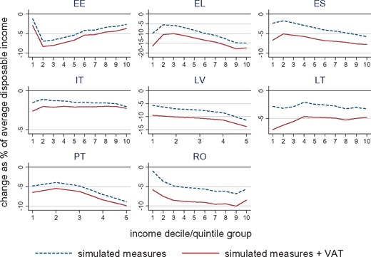
Percentage change in household disposable income due to simulated household income-based fiscal consolidation measures by household income decile group
Notes: The measures included here are those that have a direct effect on household disposable income (changes to direct taxes, cash benefits and public sector pay) and increases in the VAT rate(s). Deciles are based on equivalized household disposable income in 2012 in the absence of fiscal consolidation measures and are constructed using the modified OECD equivalence scale. The charts are drawn to different scales, but the interval between gridlines on each of them is the same. Source: own calculations with EUROMOD.
Looking at the design of the austerity measures (Table 3), in four countries (Estonia, Greece, Spain, and Italy) tax increases represent roughly 50% or more of aggregate austerity measures even without the VAT changes (the first column). At the other extreme, in Romania the net effect of tax changes resulted in lower tax revenue due to a substantial erosion of the tax base stemming from cuts in public pensions. Including VAT (the second column) shifts the overall balance between cuts in public transfers and tax increases further towards the latter. Public wage and benefit cuts remain clearly a dominant source of consolidation in Portugal and Romania (70% or more), while tax increases account for 67–74% of consolidation in Estonia, Greece, Spain, and Italy. Unlike other countries, Lithuania and Latvia have roughly an equal mix. Nevertheless, there is no clear association between the design of the austerity measures and the change in inequality of disposable income.
The design of austerity measures and effect on inequality
| Austerity measures design | Effect on Inequality | ||
|---|---|---|---|
| % of austerity measures as taxes | % of austerity measures as taxes, including VAT | % change in P90/P10 | |
| Estonia | 57.29 | 67.31 | 3.69 |
| Greece | 60.44 | 69.19 | −11.64 |
| Spain | 48.30 | 67.24 | −3.79 |
| Italy | 65.64 | 73.58 | −0.43 |
| Latvia | 35.64 | 51.27 | −4.31 |
| Lithuania | 10.92 | 48.32 | 0.40 |
| Portugal | 5.52 | 20.83 | −4.55 |
| Romania | −9.81 | 30.41 | −4.85 |
Source: own calculations with EUROMOD.
To have a better understanding of the extent to which the design of the austerity measures is related to their distributional pattern, Fig. 2 shows the variation in disposable income due to tax increases and cuts in public transfers by income decile groups. It is important to note that the tax increases are net of any automatic tax reductions due to public sector pay cuts or other taxable benefits. The overall effect from cuts of public transfers tends to be progressive in all countries but Estonia. The main drivers of such a distributional pattern are public wage cuts which show a strong progressive pattern while cuts in public pensions and other benefits show mixed results (see Fig. A3 in the online Appendix). The large size of the public sector wage cuts drives the overall progressivity observed in Greece, Latvia, and Romania and determines the contributions of those at the top of the income distribution in Portugal. The distributional incidence of cuts to public pensions depends on the design of the changes and the location of pensioners in the income distribution. In most of the countries where public pensions were reduced, this was implemented in the form of suspending pension indexation and freezing their nominal values (with higher losses for the pensioners in the lower-middle decile groups as in Spain and Latvia) or limiting the indexation for higher pensions (with losses larger in percentage terms in the middle and top of the distribution than at the bottom, as in Greece, Italy, and Portugal). In Estonia, the change in the indexation of public pensions resulted in the average pension being almost 10% lower in 2012 than it would have been otherwise, with a regressive effect because of the location of pensioners towards the bottom of the distribution. Cuts to non-pension benefits are notable only in a few countries though their incidence across the income distribution is very diverse (progressive in Latvia, regressive in Portugal, flat in Lithuania). There are important interactions in all countries, in the form of means-tested benefits absorbing part of income losses due to other instruments. However, this is only evident for countries like Estonia (where social assistance was also made more generous), Spain and Romania; while in other countries the negative effect from cuts in non means-tested benefits (Greece, Lithuania) or even in means-tested benefits themselves (Portugal) dominates.
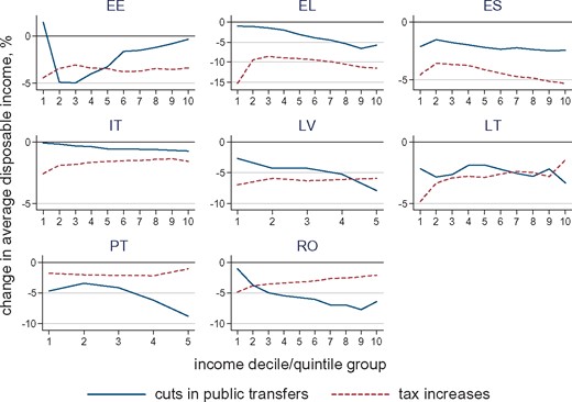
Percentage change in household disposable income due to cuts in public transfers and tax increases by household income decile group
Notes: See Fig. 1.
On the revenue side, the pattern of the distribution of tax increases is regressive in Lithuania and Romania but is generally quite flat in other countries with the exception of the larger burden faced by individuals in the first decile in several instances. In the case of the Baltic countries, small progressive increases from worker contributions are balanced with small regressive tax increases. Stronger progressive effects can be seen for Greece (with the exception of the first decile group) and Spain, where the tax increases are incident mainly on the top decile group.
4. Micro-based insights on the macro-economic effects of austerity policies
It is widely recognized that the way fiscal consolidation is achieved has implications for the prospects for macro-economic recovery and financial stability. In this context, the controversy regarding the impact of fiscal consolidation on economic output (i.e. fiscal multipliers) has dominated the academic and policy debate since the outset of the Great Recession. Nowadays it is broadly agreed that the short term effects of fiscal consolidation measures are more severe than originally thought, with fiscal multipliers (i.e. the output loss associated with a percentage point of fiscal consolidation) ranging between 0.9 and 1.7 rather than the assumed 0.5 at the beginning of the crisis (IMF, 2012; Blanchard and Leigh, 2013).
The debate on the fiscal multipliers is about the consequences of the fiscal consolidation measures on the intensity of the economic crisis which are two aspects clearly linked at least in the short term. On the one hand, austerity measures can result in a fall in aggregate demand with wider consequences for the economy in terms of firms’ output, salaries and jobs availability. On the other hand, a depressed level of economic activity can undermine the effects of the austerity measures in terms of deficit reduction. Nevertheless, Blanchard and Leigh (2013, p. 20), stress that ‘the short term effects of fiscal policy on economic activity are only one of the many factors that need to be considered in determining the appropriate pace of fiscal consolidation for any single country’.
Building on the detailed counterfactual established in the previous section, we explore the extent to which austerity measures impact directly on the aggregate level of demand of the household sector. In other words, we provide an estimate of how the decrease in real income due to such measures is transmitted through to reduction in expenditures for goods and services in a partial equilibrium setting. It seems reasonable to assume that the channel through which the distributional impact of fiscal adjustments is likely to matter the most for macro-economic performance is the effect on aggregate demand. Consumption patterns usually differ between income groups with low-income households showing a much larger marginal propensity to consume than affluent households (Jappelli and Pistaferri, 2010, 2014; Parker, 2011).
Following Auerbach and Feenberg (2000) one can assume that if the income shock is perceived as transitory and households can borrow, their demand does not change. However, according to Auerbach and Feenberg (2000) and Galì et al. (2007) it is also usual to assume that households who face liquidity constraints fully adjust consumption expenditure after changes in disposable income or, in other words, consume their entire after-tax income each year (Clinton et al., 2011). Our identification of the liquidity (and credit) constrained households follows the usual practice in the micro-based literature (Jappelli et al., 1998) and uses survey questions to define who is liquidity constrained. In our analysis, we consider liquidity-constrained households to be those who declare themselves as not having ‘the capacity to face unexpected financial expenses’ (see Dolls et al., 2012, for a robustness check with respect to the alternative questions included in the Survey of Consumer Finances). Given the estimates found in the literature (Jappelli et al., 1998), the identification of liquidity-constrained households through direct survey evidence represents an upper bound.5 We rely on the information included in the EU-SILC 2011 to predict the probability of being liquidity constrained in 2012 given income and other socio-economic characteristics of the household and taking into account the simulated effects of austerity measures and labour market adjustments. The percentage of liquidity-constrained individuals ranges from around 35% in Greece, Spain, Italy, and Portugal to 76% in Latvia (see Table 4) showing an increasing trend since the beginning of the economic crisis.6
Percentage of liquidity-constrained individuals and incidence of austerity measures
| % of liquidity- constrained individuals | % of austerity measures on liquidity-constrained individuals | % of austerity measures, including VAT, on liquidity- constrained individuals | |
|---|---|---|---|
| Estonia | 42.18 | 35.93 | 35.38 |
| Greece | 34.48 | 15.86 | 17.80 |
| Spain | 33.01 | 19.50 | 22.27 |
| Italy | 35.57 | 20.25 | 23.11 |
| Latvia | 75.93 | 59.80 | 60.38 |
| Lithuania | 61.66 | 49.83 | 51.29 |
| Portugal | 30.16 | 16.57 | 17.42 |
| Romania | 53.82 | 45.36 | 44.95 |
Notes: Liquidity-constrained individuals based on the out-of-sample prediction of the probability of being liquidity constrained taking into account the simulated effects of austerity measures and labour market adjustments. Per cent of austerity measures in terms of the aggregate revenue. Source: Own calculations with EUROMOD.
In aggregate terms, liquidity-constrained individuals face a relatively small share of total austerity measures (taking into account VAT increases as well), ranging from less than 20% in Greece and Portugal to 35% in Estonia and 45% in Romania, while in Lithuania and above all in Latvia, most of the austerity measures fall on their shoulders.
Assuming that households who face liquidity constraints fully adjust consumption expenditure after changes in disposable income, we can derive a lower bound for the effect on aggregate household demand as the effect of fiscal consolidation measures faced by the liquidity constrained (Table 5).7 The potential impact on aggregate demand, considering the effects of increases in indirect taxes as well, is highly diverse and ranges from less than 1% (of total household disposable income) in Italy to more than 7% in Latvia.
Potential reduction in the aggregate demand due to austerity measures
| Austerity measures faced by liquidity-constrained households as % of total household disposable income | ||
|---|---|---|
| Excluding VAT | Including VAT | |
| Estonia | 1.43 | 1.84 |
| Greece | 1.86 | 2.68 |
| Spain | 0.86 | 1.55 |
| Italy | 0.33 | 0.49 |
| Latvia | 5.52 | 7.36 |
| Lithuania | 1.46 | 2.59 |
| Portugal | 1.14 | 1.43 |
| Romania | 2.59 | 4.05 |
Source: Own calculations with EUROMOD.
In order to explore the potential channels through which fiscal consolidation can affect aggregate demand, and assuming that variation in income translates into a reduction in household consumption due to liquidity constraints, we look at the associations between the size and the design effects and the probability of being liquidity constrained. Table 6 shows the results of ordinary least squares (OLS) regressions where the probability of being liquidity constrained is regressed over a measure of the size and the design of austerity measures. From the results it emerges that the size of the austerity measures (expressed as a percentage of household disposable income) is negatively correlated with the probability of being liquidity constrained in all countries except Estonia and Romania. This is expected given the distributive pattern of the austerity measures, being progressive in all countries but Estonia and Romania (showing a somewhat U-shaped pattern). The design effect, in turn, shows that a greater reliance on taxes is also associated with a lower probability of being liquidity constrained, in other words households more likely to be liquidity constrained tend to be more affected by cuts in public transfers rather than tax increases. It is important to bear in mind that cuts in public transfers include both reductions in public sector pay and in benefits, the latter often being an important source of income for liquidity-constrained households. Assuming that liquidity-constrained households are more responsive in terms of consumption to income shocks, then cuts in public transfers can be seen as having more detrimental effects on aggregate demand than tax increases. The same pattern is observed even controlling for income decile groups, with the exception of Estonia and Romania, which is consistent with the distributive pattern observed in those countries. Once changes in VAT are included, as expected given the regressivity of VAT, in some countries we observe that higher reliance on taxes is associated with higher probability of being liquidity constrained but the association is still negative and significant in four countries.
Size and design effects of austerity measures on the probability of being liquidity constrained
| Estonia | Greece | Spain | Italy | Latvia | Lithuania | Portugal | Romania | |
|---|---|---|---|---|---|---|---|---|
| Size | −0.12 | −1.44*** | −1.92*** | −7.19*** | −1.22*** | −0.36*** | −1.18*** | 0.61*** |
| (0.106) | (0.048) | (0.066) | (0.164) | (0.063) | (0.088) | (0.059) | (0.055) | |
| Design | −0.11*** | −0.11*** | −0.19*** | −0.01* | −0.14*** | −0.06*** | −0.25*** | −0.10*** |
| (0.009) | (0.011) | (0.006) | (0.006) | (0.007) | (0.013) | (0.012) | (0.035) | |
| Constant | 49.21*** | 57.67*** | 49.65*** | 46.71*** | 94.12*** | 65.41*** | 43.77*** | 52.13*** |
| (0.888) | (1.028) | (0.452) | (0.597) | (0.646) | (0.468) | (0.626) | (0.526) | |
| R2 | 0.03 | 0.12 | 0.12 | 0.09 | 0.10 | 0.01 | 0.13 | 0.02 |
| Controlling for income decile groups | ||||||||
| Size | −0.31*** | −0.09** | −0.30*** | −5.58*** | −0.28*** | −0.31*** | 0.06 | 1.12*** |
| (0.095) | (0.044) | (0.067) | (0.141) | (0.052) | (0.070) | (0.059) | (0.047) | |
| Design | 0.06*** | −0.08*** | −0.05*** | −0.07*** | −0.09*** | −0.08*** | −0.05*** | −0.02 |
| (0.008) | (0.009) | (0.006) | (0.005) | (0.006) | (0.011) | (0.011) | (0.028) | |
| Constant | 15.30*** | 8.86*** | 11.91*** | 31.18*** | 66.21*** | 53.04*** | 25.20*** | 61.60*** |
| (1.335) | (1.426) | (0.996) | (0.704) | (0.993) | (1.122) | (1.23) | (0.932) | |
| Controls for decile groups | yes | yes | yes | yes | yes | yes | yes | yes |
| R2 | 0.41 | 0.46 | 0.27 | 0.34 | 0.47 | 0.39 | 0.39 | 0.37 |
| Including changes in the VAT in the Austerity measures | ||||||||
| Size | −0.32*** | −0.11** | −0.16* | −5.37*** | −0.47*** | −0.12 | 0.16** | 0.70*** |
| (0.094) | (0.046) | (0.081) | (0.145) | (0.055) | (0.076) | (0.074) | (0.134) | |
| Design | 0.07*** | −0.09*** | −0.01 | −0.05*** | −0.14*** | 0.09*** | −0.01 | −0.07*** |
| (0.009) | (0.013) | (0.009) | (0.007) | (0.009) | (0.012) | (0.014) | (0.021) | |
| Constant | 14.75*** | 10.53*** | 8.80*** | 32.06*** | 72.71*** | 45.67*** | 22.96*** | 16.97*** |
| (1.415) | (1.793) | (1.430) | (0.838) | (1.240) | (1.529) | (1.590) | (2.284) | |
| Controls for decile groups | yes | yes | yes | yes | yes | yes | yes | yes |
| R2 | 0.41 | 0.45 | 0.27 | 0.33 | 0.47 | 0.39 | 0.38 | 0.37 |
| N. Obs. | 4,744 | 6,504 | 13,014 | 20,928 | 5,196 | 4,823 | 4,454 | 7,805 |
Notes: OLS regressions at household level. Dependent variable: Probability of being liquidity constraint. Size: Austerity measures as % of household disposable income. Design: % of Austerity measures as taxes. Standard errors in brackets; ***significant at 1%; ** at 5%; * at 10%. Source: Own calculations with EUROMOD.
Overall, our finding that cuts in public transfers are more likely than tax increases to affect liquidity-constrained households casts doubts over previous findings in the macro-economic literature about the effectiveness of such measures for macro-economic recovery (Alesina and Perotti, 1995, 1997; Alesina and Ardagna, 1998, 2010, 2013) and supports the view that cuts in public transfers borne by liquidity-constrained households can have potential detrimental effects (Coenen et al., 2008, 2012; Forni et al., 2010; Clinton et al., 2011).
This suggests that it is important to distinguish between reductions in general government spending and cuts in benefits targeted on households and it is not the type of policy instrument per se which matters but how it affects different parts of the income distribution. This could be another source of variation adding to relevant aspects of country heterogeneity in the context of fiscal consolidation as discussed elsewhere (e.g. Favero et al., 2011). Disaggregated data and micro-based analysis seem necessary to reach robust policy conclusions.
5. Conclusion
The design and distributional effects of fiscal consolidation measures are of great relevance, not only because inequality, and any driver of growth in it, matters in its own right, but also because they have implications for the effectiveness of policy for macro-economic recovery.
We contribute to the literature on fiscal consolidation by estimating the distributional effects of recent policy reforms in eight EU countries which were intended to reduce budget deficits. Using the microsimulation approach, we identify and quantify fiscal consolidation measures introduced through cuts in cash benefits, increases in direct and indirect taxes and workers’ social contributions and cuts in public sector pay. Our ‘bottom-up’ measure shows that there is wide cross-country variation in the scale of the resulting aggregate reduction in household monetary resources (from 2% to 15%), and in the combinations of policy instruments that were adopted, resulting in variation in the distributional profiles of income losses. Most are progressive on the whole, although it should be emphasized that even if the poor contribute a lower proportion of their income than the rich, in some countries the scale of the reductions in their income is still large (e.g. in Greece). Including the effect of increases in VAT, which have been introduced in all the countries, reduces any progressive effect. The latter are also substantial in absolute terms, in several countries being of similar magnitude to the changes resulting from the measures affecting household incomes directly.
The distributional pattern of austerity measures is not only relevant in its own right but can also have important implications for macro-economic prospects. Based on previous episodes of fiscal consolidation over the period 1971–2009, Kaplanoglou et al. (2013, p. 7) conclude that ‘ameliorating the effects of adjustment on the weaker parts of society is crucial and … “fair fiscal adjustments” [may] provide the double dividend of promoting social cohesion, and enhancing the probability of success of the adjustment’.
The distributional impact of fiscal adjustments can matter for macro-economic dynamics, for example, through the effect on aggregate demand as consumption patterns usually differ between income groups. More disaggregated data and micro level modelling are needed in order to provide indications for the macro-economic performance of the fiscal adjustments. Our finding that combined cuts in public wages and transfers are more likely to affect liquidity-constrained households shows that these measures are not necessarily less detrimental for aggregate demand and thereby more effective than increases in taxes. This suggests that it is not the type of policy instrument per se which matters but how it affects different parts of income distributions, hence emphasizing the need to consider more disaggregated data to reach robust policy conclusions.
In interpreting our analysis there are some caveats to be borne in mind. Most importantly, our analysis does not include the impact of cuts in in-kind benefits and services on specific households. These would require additional information on the way in which cuts in public spending translate into a reduction of services available for households by their characteristics. Such data are not available in a comparable way across countries.
Supplementary material
Supplementary material – the Appendix – is available online at the OUP website.
Funding
This work was supported by the European Commission through the Social Situation Monitor; and the Economic and Social Research Council (ESRC) through the Research Centre on Micro-Social Change (MiSoC) at the University of Essex [grant number ES/L009153/1].
Acknowledgements
We are grateful to the Editor, two anonymous referees, S. Avram, C. Leventi, H. Levy, J. Navicke, M. Matsaganis, E. Militaru and O. Rastrigina for their help. We would also like to thank A. Brandolini, F. Bourguignon, H. Immervoll as well as the participants of the 8th Winter School on Social Cohesion and Public Policy (Canazei, 2013), the IZA Workshop on the Future of Labor (Bonn, 2013), the 2013 LIS Summer Lecture (Luxembourg), the 5th Meeting of ECINEQ (Bari, 2013), the 2013 ImPRovE Conference (Brussels), the 2016 York Fiscal Policy Symposium for their useful comments. We use EUROMOD F6.0 and acknowledge the contribution of all past and current members of the EUROMOD consortium. We use microdata from the 2008 EU Statistics on Incomes and Living Conditions (EU-SILC) made available by Eurostat under contract EU-SILC/2011/55 (for Latvia, Lithuania, Portugal and Romania) and the national 2008 SILC data made available by respective national statistical offices (for Estonia, Greece, Spain, and Italy).
It should be noted that there are some differences between early studies in terms of whether some items have been considered as part of spending or tax adjustments. For example, Alesina and Perotti (1995) include cash transfers in spending, while Blanchard and Perotti (2002) deduct these from taxes.
See https://www.euromod.ac.uk/using-euromod/country-reports (last accessed on 30 September, 2016).
For example, see Immervoll et al. (2011), Dolls et al. (2012), Bargain et al. (2014).
The prime examples of the EU-level policy analysis with EUROMOD are its regular use for the Social Situation Monitor (http://ec.europa.eu/social/main.jsp?catId=1049& – last accessed on 4 August, 2016) and increasing occurrence in annual country assessments as part of the European Semester (http://ec.europa.eu/economy_finance/eu/index_en.htm – last accessed on 4 August, 2016). In addition, EUROMOD has been applied in numerous policy analyses at the national level.
In addition to the effects on household spending capacity, liquidity constraints might cause the recession to be deeper and more prolonged through their effects on firm productivity. As supported by recent empirical evidence, credit to enterprises is positively and significantly associated with economic growth (Beck et al., 2012), while the effect of household credit on economic growth seems ambiguous.
According to the SILC in 2008 the share of liquidity constrained individuals ranged from around 20% in Estonia to 57% in Latvia.
The implications for the overall aggregate demand can be different in a general equilibrium setting taking into account, among other factors, changes in government debt, future expectations, factor costs, sovereign risk, cross-country linkages, and monetary policy as shown, e.g. in Coenen et al. (2008), Clinton et al. (2011), and Anderson et al. (2015).
The full list of tax-benefit instruments simulated in EUROMOD for each country, the order of calculation and underlying rules in a given year are documented in EUROMOD Country Reports (available at https://www.euromod.ac.uk/using-euromod/country-reports/ – last accessed on 4 August, 2016). All components of household disposable income are also indicated in EUROMOD Statistics on the Distribution and Decomposition of Disposable Income (see https://www.euromod.ac.uk/using-euromod/statistics – last accessed on 4 August, 2016).
References
Appendix 1: Formal presentation of modelling approach
To present our modelling approach in more formal terms, we draw on the framework suggested in Bargain and Callan (2010) for decomposing (observed) changes in the income distribution over time and its adaption in Figari et al. (2015) to a broader range of tax-benefit microsimulation applications. Following the latter, we denote labour market (and socio-demographic) characteristics of a given household with a vector c and household original income with a vector x. (We omit a subscript denoting the household.) Household original income consists of income from private and public employment, self-employment, property, investments etc, , which are separately recorded in the input data. Where relevant below, we distinguish public wages from other components of original income .
Each component – such as personal income tax, property tax, child benefit and social assistance to name a few – is calculated in steps that closely follow actual policy rules. The rules are often complex and highly non-linear and modelled in as much detail as possible given the information on relevant individual and household characteristics available in the input datasets. The list of individual instruments and the order of their calculation are specific to the country and the period in question.8 Furthermore, the nested summation-term in eq. (2) captures potential interactions between instruments (e.g. a benefit might be means-tested on the basis of income net of taxes, some non means-tested benefits are taxable), indexed by j, which in turn determine the order of calculations in a given country.
The first term on the right hand side of eq. (3), , represents disposable income in 2012 simulated according to actual policy rules and (projected) household characteristics and original incomes (including cuts and freezes in public wages). The second term on the right hand side, , is our counterfactual disposable income in 2012 with pre-consolidation tax-benefit policy rules (after adjusting monetary values of policy parameters, , according to statutory indexation rules A) applied to the same household characteristics and original incomes apart from public wages , which have been adjusted to reflect their counterfactual levels without enacted cuts and freezes. The difference between the two terms is our estimate of the effect of fiscal consolidation measures on disposable income at the household level. In Bargain and Callan’s (2010) terminology, we estimate the policy effect conditional on end-period household characteristics. This is not to be confused with the redistributive properties of a given tax-benefit system, which focuses on how the distribution of x and y differ from each other.
