


Abstract
Stereotactic radiosurgery (SRS) for the treatment of brain metastases delivers a high dose of radiation with excellent local control but comes with the risk of radiation necrosis (RN), which can be difficult to distinguish from tumor progression (TP). Magnetization transfer (MT) and chemical exchange saturation transfer (CEST) are promising techniques for distinguishing RN from TP in brain metastases. Previous studies used a 2D continuous-wave (ie, block radiofrequency [RF] saturation) MT/CEST approach. The purpose of this study is to investigate a 3D pulsed saturation MT/CEST approach with perfusion MRI for distinguishing RN from TP in brain metastases.
The study included 73 patients scanned with MT/CEST MRI previously treated with SRS or fractionated SRS who developed enhancing lesions with uncertain diagnoses of RN or TP. Perfusion MRI was acquired in 49 of 73 patients. Clinical outcomes were determined by at least 6 months of follow-up or via pathologic confirmation (in 20% of the lesions).
Univariable logistic regression resulted in significant variables of the quantitative MT parameter 1/(RA·T2A), with 5.9 ± 2.7 for RN and 6.5 ± 2.9 for TP. The highest AUC of 75% was obtained using a multivariable logistic regression model for MT/CEST parameters, which included the CEST parameters of AREXAmide,0.625µT (P = .013), AREXNOE,0.625µT (P = .008), 1/(RA·T2A) (P = .004), and T1 (P = .004). The perfusion rCBV parameter did not reach significance.
Pulsed saturation transfer was sufficient for achieving a multivariable AUC of 75% for differentiating between RN and TP in brain metastases, but had lower AUCs compared to previous studies that used a block RF approach.
Magnetization transfer and chemical exchange saturation transfer MRI can distinguish radiation necrosis from tumor progression.
Sufficient radiofrequency saturation using a continuous-wave approach is necessary.
Stereotactic radiosurgery (SRS) for the treatment of brain metastases delivers a high dose of radiation with excellent local control but comes with the risk of radiation necrosis (RN), which can be difficult to distinguish from tumor progression (TP). Magnetization transfer (MT) and chemical exchange saturation transfer (CEST) are promising techniques sensitive to tumor metabolism and microstructure for distinguishing RN from TP in treated brain metastases. Previous studies demonstrate high accuracy with a 2D continuous-wave MT/CEST approach. The present study extended the previous one to 3D, using a different sequence design incorporating a pulsed saturation MT/CEST approach, to determine its ability, along with perfusion MRI, for distinguishing RN from TP in brain metastases. The pulsed saturation approach may also allow for translational significance with a broader clinical application of RN/TP differentiation. Results showed that MT/CEST in combination with perfusion MRI helps in determining brain metastasis outcomes compared to standard MRI methods.
Stereotactic radiosurgery (SRS) delivers a high dose of radiation for the treatment of brain metastases (BM).1–3 Despite improving intracranial control,4 a fraction of patients may develop tumor progression (TP) or the high dose can lead to radiation necrosis (RN) in up to 5–25% of patients.5 Lesion enhancement in RN is similar to TP,6 and it is challenging based on standard MRI scans alone (ie, pre/post-gadolinium T1-weighted, T2-weighted, and/or fluid-attenuated inversion recovery [FLAIR]) to differentiate RN from TP without at least several months of follow-up.7 Accurate and timely diagnosis of TP or RN may influence clinical management,8 helping to guide optimal therapy including the need for resection and/or re-irradiation, or the use of steroids or anti-angiogenic therapy.
In the past, PET9 and SPECT10 have been used to distinguish TP from RN. These techniques have the advantage of being sensitive to metabolism but suffer from low spatial resolution. Early studies include diffusion MRI11,12 and magnetic resonance spectroscopy (MRS).13,14 Perfusion MRI15,16 is promising for evaluating tumor lesions and has demonstrated variable efficacy for differentiating RN from TP in glioma17 and in BM.18 In 30 BM subjects with previous SRS treatment, Kuo et al.19 have demonstrated promising results from dynamic susceptibility contrast (DSC) perfusion. However, more investigation is needed for these techniques to be fully implementable in the clinical setting.
Recently, continuous-wave saturation transfer MRI, including chemical exchange saturation transfer (CEST) and magnetization transfer (MT),20–22 have been able to differentiate RN from TP in BM patients with high accuracy.23,24 CEST MRI25,26 is capable of indirectly detecting, in low concentrations, exchangeable protons including those of amide groups that exist in endogenous proteins and peptides. MT/CEST have shown promise in numerous applications of central nervous system tumors including tumor grading,27,28 predicting correlation with genetic signatures,29,30 and therapy response assessment.31–37 In glioma, amide proton transfer (APT) CEST improves the accuracy, compared to perfusion MRI, for identifying low-grade tumors that mimic high-grade tumors as well as for differentiating TP from treatment-related effects in glioblastoma.38,39 Another study combining perfusion, diffusion, and MRS in glioma patients with prior radiotherapy has demonstrated perfusion imaging to be more reliable for differentiating between TP and RN, compared to proton MRS or diffusion.16 With the exception of several studies of BM lesions23,24,32 and one that included both glioma and BM,37 the above-mentioned CEST studies investigated only gliomas.26–31,33–36,38,39
Previous MT/CEST studies for differentiating RN from TP have been demonstrated only in a single MRI vendor using a block RF saturation pulse and a 2D approach.23,24 To ensure adequate MT or CEST saturation, the pulse sequence requires an RF pulse with a long duration on the order of seconds (ie, continuous wave), with the pulse on for the entire duration using a so-called rectangular or “block.” However, due to limitations in the RF amplifiers in certain scanners, this cannot always be achieved and instead, a “pulsed” (ie, on and off) approach is used, albeit resulting in less MT/CEST saturation. The ability to use pulsed saturation instead of a block pulse for differentiating RN from TP may allow for broader clinical applications, including scanners with hardware that cannot sustain a continuous RF pulse for long durations.37,40 The present study extended our initial study of BM lesions24 to another MRI vendor using a pulsed RF saturation technique (ie, train of Gaussian pulses) for 3D MT/CEST. To our knowledge, this study is the first where a combination of quantitative (qMT), CEST, and perfusion MRI in BM lesions is performed to help distinguish RN from TP. We evaluated qMT/CEST with the relative cerebral blood volume (rCBV) measurements obtained from DSC perfusion MRI to gather complementary information toward the development of a predictive model. qMT and CEST parameters were assessed in 73 patients, with the rCBV from DSC-MRI in a subset (49 patients), for distinguishing RN from TP.
Materials and Methods
Study Design
This study was approved by the Institutional Research Ethics Board (REB #2621). Informed consent was obtained. Recruitment included patients with BM, previously treated with SRS or fractionated SRS, with lesions indeterminate between RN and TP. Clinical outcomes were determined by a radiation oncologist, after at least 6 months of clinical and radiologic follow-up unless via pathology confirmation after MT/CEST imaging. If a lesion required resection (with pathologic confirmation of residual/recurrent tumor) or retreatment with radiation after the MT/CEST scan, then the clinical outcome was classified as TP. A diagnosis of RN was based on pathology confirming RN without active tumor, or radiographic follow-up demonstrating stability or contraction of the lesion without retreatment. The decision to retreat was undertaken when there was sufficient evidence that the lesion was in fact tumor—this required one or a combination of histopathology, serial MRI that clearly identified a growing mass, or perfusion imaging with high rCBV. Changes in lesion size over follow-up scans were assessed visually and also by the lesion measurements reported by neuroradiologists based on the post-contrast T1-weighted image. Neuroradiologists had reported on all the diagnostic imaging as per standard of care. Then, a single observer, a radiation oncologist with more than 10 years of experience, utilized neuroradiology reports to determine TP or RN outcomes. Lesions were considered indeterminate on standard MRI if there was an observed increase in the contrast-enhancing lesion on serial follow-up without a clear indication that there was tumor recurrence or progression. The research scans for this cohort were acquired between June 2021 and June 2023.
MRI Acquisition
Whole-brain saturation transfer-weighted scans were acquired with a prototype MT/CEST sequence at 3T (MAGNETOM Prisma; Siemens Healthcare, Erlangen, Germany). The saturation pulse train for MT/CEST consisted of 10 Gaussian pulses of 90-ms duration with 2.5-ms inter-pulse delay. MT/CEST scans were acquired with multiple saturation B1 amplitudes (2.5 and 3.5 µT continuous-wave power equivalent for qMT; 0.625 and 2.5 µT for CEST), slightly increased from that in our previous work to better match the CEST Z-spectrum magnetization transfer ratio (MTR) contrast. The saturation duration was chosen to approximately match our previous work.24 This study was started before the consensus recommendation41 of 2 s has been published. For MT, 11 logarithmically spaced frequency offsets were acquired between 3 and 300 ppm. For CEST, 27 offsets were acquired between ±6 ppm (at intervals of 0.25 ppm near the amide/NOE peaks between ±2.5 and ±4.5 ppm, and 0.5 or 1.0 ppm intervals outside of the amide/NOE peaks). Reference scans were collected at 783 ppm. The frequency-offset list is provided in Supplementary Table 1. Structural sequences included 3D pre-/post-contrast T1-weighted and precontrast FLAIR scans. If available, the post-contrast scans from the patient’s clinical examination were used. B0/B1/T1/T2 mapping was performed to support model fitting. The total acquisition time was 51 min. All MT/CEST MRI scans had 2 mm isotropic resolution and whole-brain coverage.
DSC perfusion imaging was performed with an echo-planar imaging (EPI) readout. The majority of perfusion scans were conducted as part of a separate diagnostic examination. For the gadolinium contrast injection, there was leakage correction in the form of preloading42 where half of the total dose by weight (0.1 mmol/kg) was given immediately before the perfusion scan, with the rest of the dose given at the start of the sixth phase of the scan. The majority of perfusion scans (47/49) were done as part of patients’ clinical examinations (ie, in a different imaging session from the MT/CEST scan, with a median interval of 6 weeks apart). Two perfusion scans were done in the same session as MT/CEST. The imaging parameters for MT/CEST/DSC perfusion are summarized in Supplementary Table 1.
Image Processing
Tumor regions of interest (ROIs) were drawn in 3D over the enhancing regions and any centrally hypointense regions. Automatic white-matter (WM) segmentation was performed with FSL FAST43 after brain extraction with HD-BET.44 Post-contrast T1-weighted (T1C) scans were coregistered to the MT/CEST maps.
For the subset of 49 patients (91 lesions) with DSC perfusion scans, the scanner-generated rCBV maps were coregistered to MT/CEST maps and normalized to a normal-appearing deep WM region in the same patient. The WM regions were selected to have a consistent ROI size (of 5 × 5 × 5 voxels) and chosen to be in the contralateral side of the lesion (or in an unaffected area of the brain). As the DSC coverage in the superior–inferior direction was limited, lesions outside of the slab were omitted from the rCBV quantification.
Statistical Analysis
MT/CEST parameters only.—
Welch’s 2-sample t-test was computed for each parameter. Univariable and multivariable analyses were used for evaluating the MT/CEST parameters for predicting RN versus TP. Statistical analysis was performed using R software (v4.3.1x64: R Core Team, Vienna, Austria).
For univariable logistic regression, the AUC and Akaike information criterion (AIC) were obtained. The AIC measures the model fit while penalizing overfitting and is useful for comparing different models with a lower AIC indicating better performance.
All available data were used to train the final multivariable logistic regression model. A bidirectional (both forward and backward) stepwise parameter selection method was used to generate the most parsimonious multivariable logistic regression model using the AIC as the selection criterion, and cross-validated AUCs were computed. To address the issue of potential overfitting with stepwise selection, competing models were generated through 10-fold cross-validation, and the model with the best performance only after cross-validation was chosen as the final model. Performance statistics for the final model were calculated in the overall cohort. A P-value below .05 was considered statistically significant. For patients with repeated scans, 1 representative scan was selected (eg, closest in time and prior to pathology) to reduce bias from correlated lesion values. To address the issue of certain groups of predictor variables showing high intragroup correlation, principal component analysis (PCA) was applied for dimensional reduction within these groups. Separate multivariable logistic regression was performed using the principal components instead of individual predictor variables from these groups to see whether the principal components showed better predictive ability.
Calibration and net benefit plots for the multivariable stepwise AIC models (without and with PCA) with the best performance after cross-validation were also generated using the “gmish” package in R (v4.3.1x64: R Core Team, Vienna, Austria). The net benefit of a model is defined as the fraction of patients treated correctly minus those treated incorrectly, where the latter is weighted by the odds of the risk threshold (also called the threshold probability) to choose treatment, normalized by the total sample size.45 This is plotted versus the risk threshold.
MT, CEST, and relative cerebral blood volume perfusion parameters.—
Since perfusion was only performed on a subset of patients, multiple imputation or “mice” package in R (v4.3.1x64: R Core Team, Vienna, Austria) was used to fill in the data using 20 imputation datasets before analyzing in combination with MT/CEST parameters. PCA was applied to reduce each of the apparent exchange-dependent relaxation (AREX) and MTR parameters to remove collinearity. Univariable and multivariable analyses were performed. Additional analyses included the subset of 30 lesions with histopathology confirmation of RN and TP.
Results
Clinical outcomes were obtained for 86 patients (185 lesions) with BM who were scanned with MT/CEST after prior SRS or fractionated SRS treatment. A total of 13 patients (36 lesions) were excluded for the following reasons: insufficient follow-up (2 patients, 3 lesions); scan issue (7 patients); lesions with indeterminate outcomes (3 patients, 3 lesions); and a patient with only hemorrhagic lesions (1 patient, 30 lesions). After exclusion, there were 73 patients (149 lesions) included in the analysis, as shown in Figure 1.
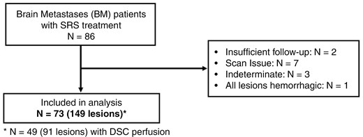
Patient flowchart. Patient characteristics are shown for the patients who were included in the analyses. N represents the number of patients.
Of the 149 lesions, 103 (69%) were classified as RN, and 46 (31%) were classified as TP outcomes. There were 30 (20%) lesions with histopathology confirmation of TP or RN. rCBV values were obtained from 91 (61%) lesions that had DSC perfusion. The patient characteristics are shown in Table 1.
Patient Characteristics
| Patient and lesion characteristics | |
|---|---|
| Number of patients | 73 |
| Median age [range] (years) | 62 [38−89] |
| Number of lesions | 149 |
| Lesions with histopathology | 30 (20%) |
| Lesions with dynamic susceptibility contrast (DSC) perfusion | 91 (61%) |
| Number of patients with repeated MT/CEST scans | 24 (33%) |
| Sex | |
| Female | 50 (68%) |
| Male | 23 (32%) |
| Lesion outcome | |
| Radiation necrosis (RN) | 103 (69%) |
| Tumor progression (TP) | 46 (31%) |
| Lesion location | |
| Supratentorial | 116 (78%) |
| Infratentorial | 33 (22%) |
| Primary tumor type (per patient) | |
| Lung | 32 (44%) |
| Breast | 21 (29%) |
| Melanoma | 10 (14%) |
| Renal cell carcinoma | 3 (4%) |
| Ovarian | 2 (3%) |
| Other (colorectal, esophagus, fallopian tube, head and neck, cholangiocarcinoma) | 5 (7%) |
| Treatment (dose/fraction) | |
| 15.0–24.0 Gy / 1 Fr | 79 (53%) |
| 21.0–27.0 Gy / 3 Fr | 9 (6%) |
| 25.0–35.0 Gy / 5 Fr | 61 (41%) |
| SRS treatment date for lesion (months before CEST scan) | |
| 6−12 months | 68 (46%) |
| 12−36 months | 62 (42%) |
| >36 months | 19 (13%) |
Characteristics of the patient cohort, including age, sex and primary tumor type, are summarized. Lesion characteristics included the outcome and radiation treatment.
Figure 2 shows parameter maps for representative patients with TP and RN. These include (i) structural images (ie, T2-weighted FLAIR images and pre- and post-contrast T1-weighted); (ii) the observed T1 and T2 from quantitative mapping; (iii) MTRAmide,0.625µT and MTRAmide,2.5µT maps which consist of a mixture of MT/CEST/T1/T2-weighting; (iv) MTRAsym,0.625µT and MTRAsym,2.5µT, which are derived from the voxelwise subtraction of MTRAmide from MTRNOE maps and which are equivalent to the APT maps commonly used in CEST literature; (v) qMT-fitted maps of R·M0B/RA (which is proportional to the semisolid fraction M0B); (vi) 1/(RA·T2A) and T2A, related to the direct effect, and (vii) AREXAmide,0.625µT and AREXAmide,2.5µT, to isolate the CEST effect from MT and direct effects.46 The nuclear Overhauser effect (NOE) maps for MTR and AREX are not shown in Figure 2 but were included in the analysis. The rCBV maps from DSC perfusion showed a hyperintense signal for the TP example and hypointense signal for the RN example.

Parameter maps for example patients. Structural images (pre- and post-contrast T1-weighted and FLAIR) and maps qMT, CEST, T1 and T2 mapping, and DSC perfusion are shown for example patients with tumor progression (top) and radiation necrosis (bottom). The ROI overlay shows the whole-tumor contours for each patient. Patients had prior SRS with radiation doses of 16 Gy in 1 fraction (top) and 25 Gy in 5 fractions (bottom).
Figure 3 shows violin plots of each (RN or TP) outcome and parameter with the median values and interquartile ranges (IQRs) listed in Table 2. Univariable analysis of the MT/CEST parameters only (Table 2) showed significant differences in the 1/(RA·T2A) qMT parameter, where RA is 1/T1 and T2A is the T2 of the free water pool from quantitative MT fitting (5.9 ± 2.7 for RN and 6.5 ± 2.9 for TP with P = .030 for t-test and P = .024 for univariable logistic regression). This was followed closely by the low-power MTR asymmetry (−1.6 ± 0.9% for RN and −1.3 ± 0.7% for TP, with P = .029 for t-test and P = .068 for univariable logistic regression) and the observed T1 relaxation time, T1 (2.0 ± 0.5 s for RN and 1.9 ± 0.4 s for TP with P = .083 for t-test and P = .11 with univariable logistic regression), which showed a trend but did not reach significance for logistic regression. The c-statistic goodness-of-fit and Brier scores for each parameter are shown in Supplementary Table 3, where lower Brier scores, between 0 and 1, indicate better calibration of predictions.
Univariable analyses
| This work | Mehrabian et al. | ||||||||||
|---|---|---|---|---|---|---|---|---|---|---|---|
| Parameter | RN | TP | Welch’s 2-sample t-test | Univariable logistic regression | RN | TP | Univariable logistic regression | ||||
| Median value [IQR] | P-value | P-value | AUC | AIC | Median value [IQR] | P-value | AUC | AIC | |||
| MTRAmide,0.625µT | 12.8 [3.1] % | 12.6 [3.9] % | .939 | .939 | 0.51 | 188.2 | 9.0 [0.9] % | 7.3 [1.4] % | <.0001 | 0.87 | 72.8 |
| MTRAmide,2.5µT | 53.3 [8.4] % | 55.1 [7.9] % | .973 | .974 | 0.51 | 188.2 | 48.2 [2.2] % | 42.2 [5.1] % | <.0001 | 0.88 | 67.3 |
| MTRNOE,0.625µT | 14.4 [3.8] % | 14.0 [3.6] % | .424 | .452 | 0.55 | 187.6 | 10.2 [1.4] % | 8.3 [1.6] % | <.0001 | 0.82 | 78.4 |
| MTRNOE,2.5µT | 52.3 [8.9] % | 52.4 [8.3] % | .744 | .751 | 0.53 | 188.1 | 46.5 [2.7] % | 41.2 [5.0] % | <.0001 | 0.83 | 77.9 |
| MTRAsym,0.625µT | −1.6 [0.94] % | −1.3 [0.69] % | .029 | .068 | 0.63 | 184.7 | −1.2 [1.3] % | −1.0 [1.2] % | .70 | 0.52 | 105 |
| MTRAsym,2.5µT | 1.8 [1.3] % | 2.1 [0.9] % | .319 | .402 | 0.61 | 187.5 | 1.7 [1.5] % | 1.2 [2.0] % | .23 | 0.58 | 103 |
| T1 | 1.95 [0.49] s | 1.92 [0.42] s | .083 | .106 | 0.56 | 185.5 | 1.77 [0.19] s | 1.94 [0.32] s | .01 | 0.69 | 98.3 |
| T2 | 179 [82] ms | 162 [88] ms | .433 | .410 | 0.55 | 187.5 | 114 [26] ms | 140 [34] ms | <.001 | 0.74 | 92.0 |
| R·M0B / RA | 0.8 [0.5] | 0.8 [0.4] | .707 | .636 | 0.46 | 188.0 | 1.4 [0.2] | 1.2 [0.3] | .009 | 0.66 | 97.6 |
| 1 / (RA·T2A) | 5.9 [2.7] | 6.5 [2.9] | .030 | .024 | 0.60 | 182.8 | 29 [4] | 26 [6] | .005 | 0.73 | 96.6 |
| AREXAmide,0.625µT | 0.040 [0.019] s-1 | 0.040 [0.025] s-1 | .250 | .250 | 0.55 | 186.8 | 2.1 [0.6] s-1 | 1.5 [0.9] s-1 | 0.002 | 0.81 | 94.7 |
| AREXAmide,2.5µT | 0.23 [0.13] s−1 | 0.25 [0.15] s−1 | .948 | .948 | 0.51 | 188.2 | 7.6 [3.2] s−1 | 5.8 [2.7] s−1 | .01 | 0.68 | 98.3 |
| AREXNOE,0.625µT | 0.052 [0.020] s−1 | 0.041 [0.024] s−1 | .874 | .878 | 0.51 | 188.1 | 2.8 [1.2] s−1 | 2.0 [0.7] s−1 | <.001 | 0.72 | 91.7 |
| AREXNOE,2.5µT | 0.19 [0.13] s−1 | 0.22 [0.12] s−1 | .670 | .684 | 0.50 | 188.0 | 5.5 [2.5] s−1 | 4.6 [2.0] s−1 | .09 | 0.62 | 102.1 |
| rCBV | 1.6 [1.3] | 1.7 [1.6] | N/A | N/A | N/A | N/A | N/A | N/A | N/A | N/A | N/A |
| After application of PCA to MTR and AREX parameters: | |||||||||||
| MTRPC1 | N/A | N/A | .922 | .929 | 0.48 | 188.1 | N/A | N/A | N/A | N/A | N/A |
| MTRPC2 | N/A | N/A | .251 | .296 | 0.57 | 187.1 | N/A | N/A | N/A | N/A | N/A |
| AREXPC1 | N/A | N/A | .066 | .098 | 0.56 | 185.3 | N/A | N/A | N/A | N/A | N/A |
| AREXPC2 | N/A | N/A | .051 | .054 | 0.62 | 184.2 | N/A | N/A | N/A | N/A | N/A |
The median and interquartile ranges are shown for the radiation necrosis (RN) and tumor progression (TP) cohorts for each parameter. Welch’s 2-sample t-test was computed for each parameter. Univariable logistic regression was performed where the area under the receiver-operating characteristic curve (AUC) and Akaike information criterion (AIC) were obtained for each parameter. The values from Mehrabian et al.24 are also shown to allow for direct comparison of the results. Values with P-values below .05 are bolded.
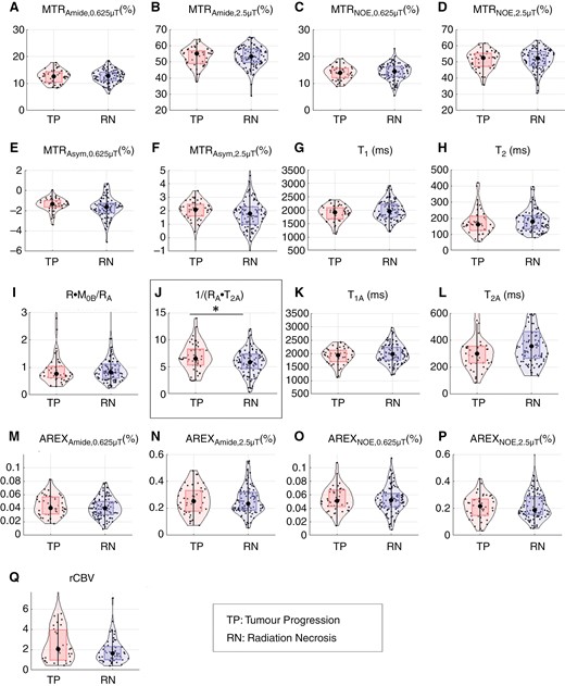
Violin plots of quantitative MRI parameters for tumor progression and radiation necrosis groups. Violin plots are shown for the tumor progression (TP) and radiation necrosis (RN) groups for each parameter. Dots represent lesion median ROI values. Median values and interquartile ranges (IQRs) are shown in Table 3. Significant differences from univariable logistic regression between TP and RN groups are shown with asterisks and boxed.
PCA was applied to the MTR (amide and NOE) and AREX parameter groups since the first principal component of each was able to explain the majority of the variability in the data suggesting that these parameters were highly correlated. PCA was applied to only the MTR (amide and NOE) and AREX parameter groups due to the high correlation found among those parameters. A heat map of the correlation between MT/CEST parameters is shown in Supplementary Figure 1. The application of PCA to the MTR and AREX group of 4 parameters for amide and NOE, did not result in additional significant parameters for the combined parameters.
Supplementary Figure 2 shows plots for the subset of 30 lesions with histopathology confirmation of RN and TP. Although none of the parameters were significant in this subset analysis, the direction of parameter value change between RN and TP groups reflects that of the overall cohort. Specifically, a higher median MTR asymmetry in the 1/(RA·T2A) qMT parameter for TP compared to RN was found in both the histopathology-only subset of 30 lesions and the entire cohort of 149 lesions. The speculated reason for not reaching statistical significance is that using a pulsed RF approach results in greater overlap between TP and RN values as compared to a block RF approach, especially when applied to relatively few lesions in this subset.
The results of multivariable logistic regression models are shown in Table 3. For MT/CEST parameters only, the stepwise AIC model resulted in four parameters being significant: AREXAmide,0.625µT (P = .013), AREXNOE,0.625µT (P = .008), 1/(RA·T2A) (P = .004), and T1 (P = .004) with a resulting AUC of 75% and AIC of 178.95. When PCA was applied to the MTR and AREX amide/NOE parameter groups, MTRAsym,0.625µT and 1/(RA·T2A) were significant variables, together yielding an AUC of 71% and AIC of 178.94. rCBV was included as part of the multivariable analyses after applying multiple imputation to address the missing rCBV data. rCBV did not reach significance in the multivariable step AIC model (P = .077), but the quantitative MT parameter 1/(RA·T2A) (P = .012), the observed T1 (P = .028), and the low-power CEST AREXAmide,0.625µT (P = .047) and AREXNOE,0.625µT (P = .026) parameters were significant. When PCA was applied, only the variable 1/(RA·T2A) was significant with P = .017. Multivariable analysis of only the MT/CEST parameters without PCA resulted in the highest AUC (75%).
Multivariable analyses
| Multivariable model | Significant parameters for multivariable logistic regression | Multivariable logistic regression, P-value | AUC with cross-validation | AIC |
|---|---|---|---|---|
| 1. Step AIC model | AREXAmide,0.625µT | 0.013 (*) | 0.75 | 178.95 |
| AREXNOE,0.625µT | 0.008 (**) | |||
| 1/(RA·T2A) | 0.004 (**) | |||
| T1 | 0.004 (**) | |||
| 2. Step AIC model with PCA | MTRAsym,0.625µT | 0.014 (*) | 0.71 | 178.94 |
| 1/(RA·T2A) | 0.030 (*) | |||
| Multivariable analysis including perfusion rCBV with multiple imputation | ||||
| 3. Step AIC model | 1/(RA·T2A) | 0.012 (*) | 0.67 [0.67, 0.67] | N/A |
| T1 | 0.028 (*) | |||
| AREXAmide,0.625µT | 0.047 (*) | |||
| AREXNOE,0.625µT | 0.026 (*) | |||
| 4. Step AIC model with PCA | 1/(RA·T2A) | 0.017 (*) | 0.67 [0.65, 0.69] | N/A |
Multivariable logistic regression was performed with and without perfusion rCBV values included. Principal component analysis (PCA) was used to reduce the AREX and MTR parameters in Model 2, whereas Model 1 used all the individual MT/CEST variables as input. Where rCBV was included (ie, Models 3 and 4), multiple imputation was used to deal with missing data. Significant parameters and values are bolded, and asterisks (*) and (**) indicate P-values below .05 and .01, respectively. For AUCs with multiple imputation and cross-validation, the 1st and 3rd quartile are shown in brackets.
The calibration and net benefit plots for the multivariable models in rows 1 and 2 of Table 3 are shown in Supplementary Figures 3 and 4, respectively. Both stepwise AIC models (without and with PCA) with the best performance after cross-validation show good agreement between predicted probabilities and observations (Supplementary Figure 3). The stepwise AIC model (without PCA) with the best performance after cross-validation offers the same or greater net benefit compared to the best stepwise AIC model with PCA after cross-validation across all threshold probabilities (Supplementary Figure 4). The greatest net benefit of the stepwise AIC model (without PCA) of 0.045–0.06 occurs approximately at a threshold probability between 0.4 and 0.5.
Discussion
The current study used a 3D implementation of MT/CEST with whole spectra for CEST. The total scan time was 51 min (with 6 min 3 s for MT and 10 min 51 s for CEST, per saturation amplitude) while producing whole-brain coverage with isotropic voxel size (2 × 2 × 2 mm3) and dense Z-spectrum sampling around ±3.5 ppm. Results from univariable and multivariable logistic regression showed promise for the differentiation of TP from RN in BM patients.
The number of patients in our study was similar to that of our previous study of BM lesions.24 However, major differences in the present study included a 3D MT/CEST implementation (instead of single slice), a Gaussian pulse train for RF saturation (instead of a block pulse) with RF spoiling, the addition of DSC perfusion MRI to the dataset, the exclusion of hemorrhagic regions from the whole-lesion contours, and more lesions with histopathological confirmation.
As the MTR (amide and NOE) parameters were only semiquantitative, the lack of significant differentiation in this cohort compared to our previous studies23,24 could have been related to pulse sequence differences resulting in differing contributions of MT, CEST, and the direct saturation effect. For comparison between studies using the amide or NOE MTR, it is likely that the signal needs to be modeled fully for each sequence implementation (eg, pulse train or block saturation) as part of future work by propagating the signal through the Bloch equations.
MTR asymmetry is a commonly used metric across APT studies41 and we observed higher values in TP compared to RN (consistent with higher values associated with higher glioma grades41), the parameter did not reach significance in the univariable or multivariable analyses. This may be due to higher inherent noise in this parameter compared to others.
The purpose of AREX is to remove the effects of T1 that are found in MTR. AREX was one of the predictors in the multivariable step AIC logistic regression models prior to PCA, suggesting that including AREX parameters can help for differentiation between RN and TP as shown in previous BM studies.23,24 However, the AUCs for this parameter in the univariable analyses were substantially lower (with AREX AUCs of 0.55, 0.51, 0.51, and 0.50 for Amide 0.625µT, Amide 2.5µT, NOE 0.625µT, and NOE 2.5µT, respectively, whereas Mehrabian et al.24 had AUCs of 0.81, 0.68, 0.72, and 0.62 for the same parameters). This could have been due to the following differences between the current study and that of Mehrabian et al.24:
Saturation RF pulse design: As these studies were acquired on different MRI vendors, there were inherent differences in the MT/CEST RF pulse. While a block pulse was used before,24,32 our current implementation required a pulsed approach with the major advance being a 3D sequence of similar scan times as the previous study.
RF spoiling: Spoiling between successive TRs was used only in the current study, which is recommended.47 No spoiling was used in Mehrabian et al. and could have rendered the MTR amide/NOE contrast similar to SSFP (T1/T2)-weighting in addition to MT/CEST/rNOE.
Repeated scans of the same lesion: Both studies contained patients who were scanned more than once. However, multiple scans of the same lesion, if treated as separate lesions in the analysis,24 may lead to biases as the signal cannot be considered independent. Here, only one instance of each repeated lesion was analyzed to minimize bias.
Results of the current study, in comparison to Mehrabian et al.,24 suggest that more CEST saturation (ie, using a block RF approach) is needed for accurate differentiation. A block pulse of equivalent duration to a pulse train should have a greater MT/CEST effect and subsequently greater contrast. Other improvements in the current study over the previous one24 (including the 3D acquisition, RF spoiling, not counting repeated lesions) are considered to be minor and less likely to affect the accuracy of differentiation since these affect a minority of the patients in the cohort in contrast with RF pulse differences.
This study extended our previous studies in BM23,24 by including DSC perfusion. rCBV values were available in 61% of the lesions analyzed. However, due to data availability in only a fraction of lesions, multiple imputation had to be employed in the statistical analyses before the inclusion of rCBV values with other MT/CEST parameters in the multivariable analyses. Although the rCBV parameter was not significant, TP showed higher rCBV (1.7 ± 1.6 in TP compared with 1.6 ± 1.3 in RN); the direction was consistent with literature in glioma where lesions with higher rCBV are more likely to be tumors.16 Improvements to the sequence could focus on reducing the susceptibility artifacts from air–tissue interfaces from the EPI readout used in the DSC-MRI sequence, which degraded the image quality in some cases. Other methods including arterial spin labeling for obtaining perfusion metrics can be explored in the future.48
The relatively long scan time for MT/CEST is a limitation of this work. A future extension to speed up the acquisition can be achieved by gathering a subset of the MT/CEST frequency offsets instead of the whole spectra, or by employing fast imaging approaches such as compressed sensing and parallel imaging in combination with CEST.49,50 The use of multiple imputation in 39% of patients due to missing DSC acquisition is another limitation of the study. Although multiple imputation is a popular method of filling in missing data, it may artificially reduce the variation or exaggerate the multivariate relationships in the data.51–53 See Supplementary Table 2 for additional analyses performed without multiple imputation on the subset of 91 lesions for which perfusion and MT/CEST data are available. As stated in the Methods section, multiple testing was not performed. One of the major limitations is that the variables would no longer be significant with Bonferroni correction. Stepwise parameter selection using AIC has been known to lead to poor modeling and overfitting; other methods such as LASSO may be explored but will require more data. Another limitation is that the conclusions were drawn from the entire cohort, which comprises varied patient characteristics (eg, lesion types or SRS fractionation) and could have decreased the accuracy. Future work will involve addressing model fairness and subgroup analyses with more uniform lesion characteristics; however, higher numbers for each subgroup will be necessary. The predictive model will need to be validated using a larger dataset and according to rigorous predictive modeling requirements.54
MT and CEST are promising techniques for distinguishing RN from TP in BM, but sufficient RF saturation is likely necessary for higher AUCs. This study investigated the rCBV derived from DSC perfusion. While the rCBV values reflected the trends in literature, results showed that MT/CEST parameters had greater efficacy compared to rCBV for differentiating RN from TP in BM. In conclusion, pulsed saturation transfer is sufficient for achieving a multivariable AUC of 75% for differentiating RN from TP in BM lesions. However, the pulsed RF method used in the current study had lower AUC compared to previous work that had used a block RF pulse approach.
Funding
This work was supported by the Terry Fox Research Institute (New Frontiers Program Project Grant); the Canadian Institutes of Health Research (Project Grant); and the Canadian Cancer Society.
Acknowledgments
We thank Colleen Bailey for help with patients; Andrew Stanisz for technical assistance; Fred Tam (SRI) and Gerald Moran (Siemens Healthcare) for help with pulse sequences; Dylan Young and Athavan Gananathan for assistance with various aspects of the study; Dr. James Perry and Dr. Nir Lipsman for advice and lesion information and Maged Goubran for discussions related to segmentation.
Conflict of Interest
A.S.: Elekta/Elekta AB: Research grant, Consultant, Honorarium for past educational seminars, Travel Expenses. Varian: Honorarium for past educational seminars. BrainLab: Research grant, Consultant, Honorarium for educational seminars, Travel Expenses. AstraZeneca: Honorarium for educational seminars. ISRS: President of the International Stereotactic Radiosurgery Society (ISRS). Seagen Inc: Honorarium for education seminars and research grants. Cerapedics: Honorarium for educational seminars, Travel Expenses. CarboFIX: Honorarium for educational seminars. Servier: Honorarium for educational seminars.
C.-L.T.: Travel accommodations/expenses & honoraria for past educational seminars by Elekta; belongs to the Elekta MR-Linac Research Consortium; advisor/consultant with Sanofi and AbbVie.
S.M.: Research support from Novartis AG, honoraria from Novartis AG and Ipsen. None related to this work.
Authorship statement
Study design: G.J.S., H.S., A.S., H.M., H.C. Scan methodology: R.W.C., W.W.L., P.J.M., G.J.S. Sequence implementation: P.L. Data analyses: R.W.C., W.W.L., L.M., D.D. Statistical analyses: H.C. Patient recruitment: A.S., C.L.T., S.M. (Sten Myrehaug), J.D., H.S., H.C., M.J.L.F., K.R. Informed consent: A.T. Patient scanning and support: R.E., S.M. (Sankyu Moon), R.W.C., W.W.L., L.M., A.T., B.L., D.D. Clinical information: H.S., B.Z., A.S., H.C., C.L.T., S.M. (Sten Myrehaug), J.D., H.C., M.J.L.F., K.R., B.M.K. All authors read and approved the final manuscript.
Data availability
The data, study protocol, or code will be made available upon reasonable request. The intention is for this dataset to made publicly available in the future.
References
Author notes
Rachel W Chan and Wilfred W Lam contributed equally as first authors.
Hany Soliman and Greg J Stanisz contributed equally as Principal Investigators.
