


Abstract
Littoral zone aquatic habitat is an important component of sport fish population dynamics in freshwater lakes and reservoirs and is a primary target of fisheries management actions. However, habitat data for these systems are often minimal or nonexistent due to the cost and time‐consuming nature of traditional aquatic habitat sampling methods. Side‐scan sonar has been identified as a potential tool that can address these limitations, allowing quantification of habitat features over large areas. Side‐scan sonar is available in two forms: recreational (consumer grade) and professional (survey grade). Our goal was to compare these two grades of side‐scan sonar by analyzing their ability to map littoral habitat features in three Ohio reservoirs.
We used a Lowrance Active Imaging 3‐in‐1 system (≈US$2000) recreational sonar and an EdgeTech 6205 system (≈$150,000) survey‐grade sonar to collect imagery in the littoral zones of reservoirs. We manually quantified submerged woody debris, standing timber, aquatic vegetation, and benthic substrate in a geographical information system (GIS) using imagery from each sonar system and compared habitat estimates and GIS processing times. We analyzed how differences in image resolution between the two sonar systems affected the level of variation in habitat classification values generated by individual analysts.
We found small differences in habitat classification values and accuracy between the two sonar systems, and trade‐offs existed in spatial accuracy and ability to image dense vegetation. However, side‐scan data acquisition, postprocessing, and habitat classification were generally less time‐intensive with the recreational Lowrance system than with the survey‐grade EdgeTech system. Unexpectedly, the lower quality Lowrance imagery had less user‐based variation in GIS habitat classification.
Recreational side‐scan sonar systems such as the Lowrance system provide sufficient imagery resolution, habitat classification values, and accuracy at a lower cost and with less processing time than survey‐grade side‐scan sonar systems and are useful tools for quantifying littoral habitat features in reservoirs.
Habitat is likely a critical driver of fish populations but is difficult to measure. Our project compares the utility and efficiency of readily available, low‐cost recreational sonar to those of survey‐grade sonar for use in measuring habitat features along the edges of reservoirs.
INTRODUCTION
Aquatic habitat is a critical component of sport fish population dynamics in freshwater lakes and reservoirs, and aquatic habitat improvement, inventorying, and monitoring in these systems often constitute a primary focus of fisheries managers (Fisher et al. 2012). However, traditional aquatic habitat sampling methods have several limitations. Specifically, traditional transect‐based methods of surveying aquatic habitat can be arduous and time‐intensive (Kaeser and Litts 2008, 2010). Moreover, these methods fail to provide spatially continuous data, and their implementation can often be impracticable, especially in deep or turbid environments (Richter et al. 2016). These limitations of traditional sampling methods have consistently resulted in shortages of aquatic habitat data for many freshwater systems (Richter et al. 2016; Schooley and Neely 2018).
Side‐scan sonar has been identified as a potential solution for combatting the disadvantages of traditional aquatic habitat sampling (Kaeser and Litts 2008; Richter et al. 2016). Side‐scan sonar allows for the efficient collection of spatially continuous benthic imagery in lakes and reservoirs, and its use is generally not limited by depth or turbidity (Richter et al. 2016). The first side‐scan sonar systems were produced in the late 1960s and allowed for the collection of qualitative data about the acoustic properties of the ocean floor (Johnson and Helferty 1990). Today, side‐scan sonar exists in two different forms: recreational (consumer grade) and professional (survey grade; Fleming et al. 2018). Recreational side‐scan sonar systems are widely available, low‐cost systems that are generally marketed toward anglers (Buscombe et al. 2016; Bodine et al. 2022). These systems contain minimal hardware, are notable for their ease of use (Halmai et al. 2020; Bodine et al. 2022), and do not require any external software for operation. In contrast, survey‐grade side‐scan sonar systems are relatively expensive, are hardware‐intensive, and are not widely available in the retail marketplace. Furthermore, the operation of survey‐grade sonar systems requires a significant amount of professional training and involves the use of external software to operate the equipment. The primary benefit of using a survey‐grade side‐scan sonar system is higher signal‐to‐noise imagery with greater positional accuracy than data from recreational systems (Halmai et al. 2020).
Regardless of the difference in data quality, recreational side‐scan sonar systems have accounted for the majority of ecological side‐scan sonar applications in freshwater systems. In 2008, a foundational study for the measurement of freshwater aquatic habitat was published (Kaeser and Litts 2008), in which recreational side‐scan sonar was used to measure and quantify submerged logs in a Georgia river. Since then, many studies have used recreational side‐scan sonar for the collection of aquatic habitat data. Several of these studies have focused on the classification and measurement of benthic substrates, often with reference to a specific fish species and associated spawning habitat requirements (Kaeser and Litts 2010; Kaeser et al. 2013; Powers et al. 2015; Cheek et al. 2016; Litts and Kaeser 2016; Richter et al. 2016; Walker and Alford 2016; Graham et al. 2017; Schooley and Neely 2018; Parker et al. 2020). Other studies have concentrated on the ability of recreational side‐scan sonar to quantify and map other habitat features, such as aquatic vegetation (Daugherty et al. 2015; Greene et al. 2018; Bennett et al. 2020) and woody debris (Kitchingman et al. 2013; Daugherty et al. 2015).
Many of the ecological studies using side‐scan sonar have focused on the manual classification and identification of features that are visible on the imagery. Because these manual processes inherently involve human interpretation, there is a significant potential for interpreter bias to influence survey results and accuracy (Gonzalez‐Socoloske and Olivera‐Gomez 2012; Fleming and Daugherty 2021). This interpreter bias can result in the misclassification of features during the imagery analysis process (Gonzalez‐Socoloske and Olivera‐Gomez 2012). Recently, however, there has also been a significant amount of work devoted to the automated classification and delineation of benthic substrate types by using recreational side‐scan sonar imagery (Buscombe et al. 2016; Hamill et al. 2016, 2018; Buscombe 2017; Bodine et al. 2022). This is due not only to the biological importance of benthic substrate habitats in freshwater ecosystems, but also to the difficulties and inconsistencies associated with manual delineation of substrate class boundaries on side‐scan imagery (Richter et al. 2016; Walker and Alford 2016; Graham et al. 2017).
Survey‐grade side‐scan sonar units are used less frequently in freshwater systems for fisheries applications, and most of these uses have either been in coastal rivers or in the Laurentian Great Lakes. For example, Flowers and Hightower (2013) used an EdgeTech 4125‐P dual‐frequency, survey‐grade side‐scan unit to survey Atlantic Sturgeon Acipenser oxyrinchus in several coastal rivers of North Carolina and South Carolina. Similarly, Boase et al. (2014) used an EdgeTech 4100‐P side‐scan sonar unit to survey Lake Sturgeon A. fulvescens habitat in the St. Clair River. Redman et al. (2017) used an L3‐Klein System 3000 dual‐frequency side‐scan system to map Lake Trout Salvelinus namaycush reef habitats in Lake Michigan. Otherwise, most ecological uses of survey‐grade side‐scan sonar have been in marine environments (e.g., Hewitt et al. 2004; Hartstein 2005; Teixeira et al. 2013).
The objective of this study was to compare the relative utility of recreational and survey‐grade side‐scan sonar systems for use in reservoir fisheries management. Reservoirs provide important recreational fishing opportunities to communities throughout the United States (Daugherty et al. 2015). However, aging processes, such as sedimentation, shoreline erosion, and structural habitat degradation, make reservoir management a challenging and complex endeavor (Harris et al. 2018). Moreover, reservoir managers often lack the habitat data that are required to properly inform sport fish management decisions (Daugherty et al. 2015). We wanted to determine which grade of side‐scan sonar is the more practical option for mapping and inventorying reservoir habitat features that are considered relevant for sport fish populations at the water body scale. To accomplish this task, we performed side‐scan sonar surveys of three reservoirs in southwest Ohio using a recreational Lowrance side‐scan sonar system (≈US$2000) and an EdgeTech 6205 survey‐grade side‐scan sonar system (≈$150,000, including associated equipment and software). We focused specifically on the littoral (nearshore) zone of each reservoir because nearly all reservoir fisheries sampling in Ohio is conducted in the littoral zone. Moreover, woody debris, aquatic vegetation, spawning substrates, and other physical structures, which serve as important habitat components for fish (and a variety of other organisms), tend to be found in the littoral zone (Daugherty et al. 2015; Richter et al. 2016). Therefore, littoral zone habitat composition can significantly influence both fish abundance and distribution within a lake (Ahrenstorff et al. 2009).
We sought to determine whether survey‐grade sonar substantially outperforms recreational sonar as a tool for inventorying and quantifying littoral habitat in reservoirs. Because survey‐grade sonar systems provide higher resolution side‐scan imagery with greater positional accuracy than their recreational counterparts, we expected that habitat classification accuracy and classification precision between analysts would be higher with survey‐grade side‐scan data. However, we also expected that the more detailed imagery and relatively large file sizes associated with the survey‐grade sonar data would reduce processing efficiency by increasing the amount of time required to identify and classify habitat features.
METHODS
Study sites
Data for this study were collected at three reservoirs in southwest Ohio that were specifically selected to provide imagery of a range of representative habitat features of interest. Acton Lake is a small (≈240‐ha), highly eutrophic, shallow reservoir with approximately 14.2 km of shoreline and a maximum depth of approximately 9.1 m. The northernmost portion of Acton Lake is generally nonnavigable by boat due to heavy sedimentation from the two primary tributaries to the lake and has a relatively simple shoreline, with an overflow dam and riprap wall at its southern end. Rocky Fork Lake contains approximately 50 km of shoreline, is approximately 791 ha in size, and has a maximum depth of about 12.2 m. Rocky Fork Lake was selected due to the relatively high amount of aquatic vegetation present throughout the lake. Caesar Creek Lake was the largest reservoir in this study (≈1136 ha), with 58.4 km of shoreline and a maximum depth of 35 m. Caesar Creek Lake is composed of two separate basins and is notable for its diversity of habitat types, including a significant presence of drowned standing timber. All three reservoirs typically have low visibility (Secchi depth ≤ 1 m) throughout the year. These reservoirs typically stratify during summer at approximately 5–8 m and have hypoxic conditions in the hypolimnion during the stratified period.
All three study reservoirs are monitored via standardized electrofishing surveys by the Ohio Department of Natural Resources–Division of Wildlife as part of its Inland Management System (IMS). In brief, the survey protocol divides the navigable portion of these reservoirs' littoral zones into individual sampling transects (“IMS sampling sites”) that parallel the shoreline and are approximately 500 m in length, with the number of sites dictated by the shoreline of the lake (Acton Lake: 14 sites; Rocky Fork Lake: 49 sites; Caesar Creek Lake: 92 sites). Habitat data in this study were quantified at the scale of an individual IMS sampling site.
Equipment
The survey‐grade sonar system used for this project was an EdgeTech 6205 dual‐frequency (550‐ and 1600‐kHz) side‐scan sonar and bathymetry system (hereafter, “EdgeTech system”). This sonar system simultaneously collects side‐scan sonar imagery and multi‐beam, point‐cloud swath bathymetry data. The physical components of the EdgeTech system include a submersible sonar transducer (759 × 208 × 244 mm [length × width × height]), a 6205‐R rack‐mount interface box, and a 20‐m deck cable that was used to connect the sonar head to the interface box. The sonar transducer was mounted to the starboard side of the survey boat using a rigid aluminum mast (Over‐the‐Side Mini Mount; Marine Survey Fabrication) that allowed the transducer to be tilted fore and aft as well as raised from and lowered into the water. The transducer was submerged approximately 0.3 m below the surface of the water. The EdgeTech system was paired with the Applanix POS MV SurfMaster system (Applanix), which obtains precise position, heading, attitude, heave, and velocity data. The Applanix POS MV SurfMaster system consists of two Global Navigation Satellite System (GNSS) antennas, an inertial measurement unit (IMU), and an interface box. The two GNSS antennas and the IMU were mounted in fixed positions on the boat and were connected to the interface box. An onboard dual‐monitor computer setup was used to run the sonar acquisition software programs (HYPACK 2020 [Xylem] and Discover Bathymetric [EdgeTech]). Exact positions and offsets relative to the boat's center of gravity were recorded for the sonar head, IMU, and GNSS antennas. During data collection, all equipment was powered using a 2000‐W, onboard gas‐powered generator. Approximately 30 min of equipment setup and startup time were required prior to the start of each day of EdgeTech data collection.
The recreational side‐scan sonar system used in this study consisted of a Lowrance HDS 12 Carbon fish finder/chart plotter, a Lowrance Active Imaging 3‐in‐1 sonar transducer (257 × 67 × 35 mm [length × width × height]; 800 and 455 kHz), and a Lowrance Point‐1 Global Positioning System (GPS) antenna and heading sensor (hereafter, “Lowrance system”; Navico Group). The fish finder unit powers the sonar transducer, records data on a removable memory chip, and serves as a means of visualizing the side‐scan imagery while on the boat. The Lowrance transducer was mounted on a movable pole, which was mounted in front of the bow of the survey boat, and the transducer was submerged approximately 0.2 m below the surface of the water. The transducer was mounted off the bow rather than the stern (typical install location for recreational boats) to minimize the impact of turbulence and bubbles from the outboard motor, which would reduce image quality (Kaeser and Litts 2008). Less than 5 min of equipment setup and startup time were required prior to the start of each day of Lowrance data collection.
Sonar data collection
Sonar data collection was performed in the summer of 2021 and in the spring and summer of 2022. Side‐scan sonar imagery of the littoral zone was collected with both types of sonar systems by driving the boat approximately 30–40 m offshore and parallel to the shoreline at speeds of approximately 4.5–6.5 km/h (Richter et al. 2016). All accessible areas of shoreline with IMS sampling sites (i.e., areas with sufficient depth for boat access and no navigational restrictions) were scanned. Although the EdgeTech system is capable of recording at both frequencies, due to swath width limitations at the 1600‐kHz frequency, we only used the 550‐kHz imagery. Lowrance side‐scan imagery was collected at a frequency of 455 kHz. The total swath width for both systems was set at 100 m (i.e., 50 m on either side of the boat). This range setting was a compromise between achieving the recommended depth‐to‐range ratio of 0.1–0.2 for high‐quality sonar imagery (Kaeser and Litts 2010) and minimizing the potential for crashing the EdgeTech transducer into submerged obstacles (actual depth‐to‐range ratios: Acton Lake: 0.06–0.07; Caesar Creek Lake: 0.1; Rocky Fork Lake: 0.06–0.07). During data collection, real‐time kinematic (RTK) GPS corrections were applied to the EdgeTech data using the Ohio Real Time Network. This resulted in a positional accuracy of less than 3 cm for the EdgeTech side‐scan imagery (as reported in real time by the data‐logging software). Data collected with the Lowrance system had a positional accuracy of about 3 m when paired with the Point‐1 GPS antenna (Halmai et al. 2020).
EdgeTech sonar data processing
Side‐scan sonar files collected with the EdgeTech 6205 system were processed and mosaicked by using SonarWiz 7 software (Chesapeake Technology Inc.). The bottom tracking and slant range correction functions were used to remove the water column and georectify the imagery, and empirical gain normalization and the nadir filter were applied to visually optimize the imagery. The side‐scan mosaic of the entire lake was exported as tiled GeoTIFF images.
Lowrance side‐scan data processing
Side‐scan sonar files collected with the Lowrance system were processed and mosaicked with ReefMaster version 2.0 (ReefMaster Software Ltd.). After the files were imported to the program, the water column was subsequently removed from the imagery using the “water column offset” feature. The files were then added to a mosaic, where the sharpness, gain, brightness, and contrast of the image were adjusted for optimum visibility. Lastly, the mosaics were exported as MBTiles files, which were then imported into QGIS version 3.20.1 (QGIS.org) for habitat mapping and quantification.
Manual habitat quantification
Sonar imagery was imported into QGIS version 3.20.1 for habitat analyses. A single researcher (T. Fletcher) delineated the patches of littoral zone woody debris, standing timber, aquatic vegetation, and benthic substrate that were visible in each set of sonar imagery (Figure 1). We defined the quantification area of the littoral zone as the region between the lake shoreline (using existing geographical information system [GIS] layers for lake shorelines) and 30 m out into the water using an internal buffer. We quantified the areal coverage of submerged woody debris and aquatic vegetation by delineating all visible pieces of wood and patches of vegetation as polygon features (N = 56 IMS sampling sites). If multiple pieces of woody debris overlapped with one another, they were grouped together in a single polygon to avoid double counting the area of overlap. Standing timber within the littoral zone was quantified by marking each individual standing tree or stump as a point feature (N = 42 IMS sampling sites). Areal estimates of each habitat patch type (e.g., wood or vegetation) were summed within each IMS sampling site. Since IMS sites varied to some degree in their total area due to shoreline complexity, areas were converted to percent cover and points were converted to count per 1000 m2 by dividing by the quantification area of the IMS site.
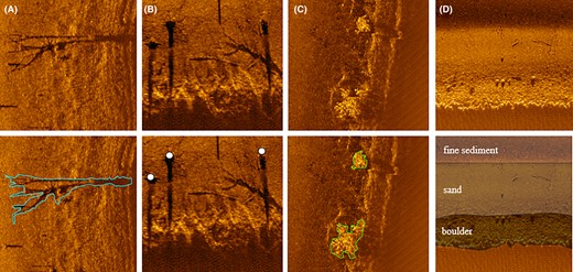
Examples of delineated habitat features: (A) submerged woody debris polygons, (B) standing timber points, (C) submerged aquatic vegetation polygons, and (D) benthic substrate polygons.
Benthic substrate was quantified by dividing a polygon of the littoral area of an individual IMS site into sections based on discernible substrate type (N = 38 IMS sampling sites). These polygon sections were given a specific classification as “boulder,” “cobble,” “gravel,” “sand,” “fine sediment,” or “other” (artificial structures; e.g., concrete boat ramps, bridge pilings, etc.). Each polygon section was also given a broad classification as “coarse,” “fine,” or “other.” The “coarse” category included areas classified as “boulder” and “cobble,” whereas the “fine” category included areas classified as “gravel,” “sand,” and “fine sediment.” The classification of “other” was the same for both the specific and broad categories. Areas of blank imagery adjacent to the shore (i.e., areas where the sonar beam failed to reach the shoreline due to shallow depth, dense vegetation, etc.) were labeled as “unclassified” (Figure S1 available in the Supplement in the online version of this article). Classification was performed using a training set of reference images of the different substrate types that were taken from areas of known substrate composition. The minimum size for all classifiable sections (i.e., sections not designated as “unclassified”) was 3 × 3 m. Within each IMS site, areas of each substrate type were summed and divided by the total area of the IMS site to obtain the percent areal coverage of both the specific and broad substrate categories. The GIS mapping times for each habitat feature were also recorded at a subset of IMS sampling sites from each lake to assess how image quality from each sonar system affected processing efficiency.
We used Wilcoxon's signed rank tests to compare Lowrance and EdgeTech site‐level habitat values for submerged woody debris, standing timber, and aquatic vegetation and to compare site‐level processing times for each habitat feature. For submerged woody debris specifically, we divided the 30‐m‐wide littoral area in half and compared the amount of submerged woody debris observed on each set of imagery in both the shoreline‐to‐15‐m zone and the 15–30‐m zone. We also used Wilcoxon's signed rank tests to compare both the number and size of individual polygons drawn in the shoreline‐to‐15‐m zone. A chi‐square test of homogeneity was used to compare the manually classified substrate compositions from the Lowrance and EdgeTech imagery. We used major axis regression to determine the relationship between the submerged woody debris, standing timber, and aquatic vegetation habitat values from each set of sonar imagery because both axes have measurement error. We estimated slopes and intercepts for each habitat feature using the package lmodel2 (Legendre 2018) in the R statistical environment (R Core Team 2024). We tested regression slopes for significance by determining whether their 95% confidence intervals included 1.0 (the confidence intervals including 1.0 indicated nonsignificance) because our null hypothesis was that the sonars do not differ in their estimate of habitat cover.
Ground‐truthing data collection
We collected ground truth data for the aquatic vegetation and benthic substrate habitats in the summer of 2022 to quantify our GIS classification accuracy for these habitat types. A subset of IMS sampling sites was randomly selected from each reservoir for ground‐truthing, and the number of sites sampled was dictated by the surface area of the reservoir (Acton Lake: 6 sites; Rocky Fork Lake: 12 sites; Caesar Creek Lake: 18 sites). Due to the high turbidity levels in the reservoirs, visual verification of habitat features was generally not possible. To combat this issue, we devised alternative ground‐truthing methods for these two habitat types. We also attempted to ground‐truth the submerged woody debris and standing timber habitats. However, the ground truth technique that was devised for these habitat types proved unreliable.
Vegetation and substrate ground‐truthing methods were based on the methods implemented by the Ohio River Valley Water Sanitation Commission (2021). For both substrate and vegetation ground‐truthing, six transects of points were collected at each IMS site. These transects were spaced approximately 100 m apart. The collection of ground truth points for each transect began at the shoreline and proceeded offshore until 11 points were recorded or until water depth exceeded the length of the rake or copper pole. To ensure the spatial accuracy (<0.1 m) of the aquatic vegetation and substrate ground‐truthing data, aquatic vegetation and substrate were measured directly below an RTK GPS receiver (Emlid Reach RS2 RTK GNSS receiver; Emlid Tech Kft.) mounted at the bow of the boat. The GPS receiver was connected via Bluetooth to a smart tablet running data collection software (QFieldCloud; OPENGIS.ch GmbH) and allowed us to record data as attributes in a shapefile layer, which could then be directly uploaded via the cloud into an existing QGIS project.
To ground‐truth aquatic vegetation, a technician standing at the bow of the boat pressed a custom‐fabricated, 3.7‐m, double‐sided rake into the lake bottom; rotated the rake twice (720°); and lifted the rake from the water. The density of aquatic vegetation covering the rake was then recorded on a qualitative scale of 0 (no vegetation present) to 3 (rake entirely covered). Two types of emergent vegetation—lily pads (Family Nymphaeaceae) and American water willow Justicia americana—were less amenable to the raking procedure, so their presence was simply recorded from visual observations without a density rating. In total, 1154 vegetation ground‐truthing points were recorded. We measured ground‐truthing accuracy for aquatic vegetation on a presence/absence basis using a point‐in‐polygon overlay in QGIS. If a ground‐truthing point that contained some level of vegetation overlapped with a manually drawn vegetation polygon, then vegetation was considered to be correctly classified at that point. Similarly, if a ground‐truthing point that contained no vegetation (score = 0) fell outside of the vegetation polygon layer, vegetation (or a lack thereof) was considered to be correctly classified at that point. We used the buffer function in QGIS to account for potential inaccuracy in the location of side‐scan imagery. Specifically, 1‐, 3‐, and 5‐m buffers were inserted around each ground truth point at a misclassified location to determine whether the misclassification could potentially be attributed to the positional inaccuracy of the side‐scan imagery. If a ground truth point at a misclassified location was within 5 m or less of an area of matching classification, then the misclassification could potentially be attributed to the positional inaccuracy of the side‐scan imagery.
Substrate ground truth readings were taken from the bow of the boat. A single technician probed the lake bottom with a 6‐m copper pole; based on the tactile and auditory sensations, the technician classified the substrate as boulder, cobble, gravel, sand, fine sediment, or any combination thereof (up to three different substrate classes). To ensure the accuracy of this method, prior to data collection, technicians performed this procedure in areas of known substrate composition and took note of the tactile and auditory responses that were characteristic of each substrate class. In total, 2121 substrate ground‐truthing points were recorded. We used a point‐in‐polygon overlay in QGIS to analyze benthic substrate classification accuracy for both sets of side‐scan sonar imagery. Classification accuracy for each specific and broad substrate class was quantified by calculating the proportion of ground truth points that overlapped polygons with matching substrate designations. For specific substrate classes, only ground truth points that contained a single type were used for assessing classification accuracy. For broad substrate comparisons, only ground truth points where all classifications were within the same category were used (e.g., points classified as cobble/sand were not used, but those classified as boulder/cobble were used). We used ground truth points as our reference to calculate classification accuracy statistics, including overall accuracy (proportion of correctly classified points), user's accuracy (proportion of correctly classified points), and producer's accuracy (correctly identified habitat features; Congalton and Green 1999). The recommended target level of overall accuracy is 85%, with a minimum of 70% accuracy per class (Anderson et al. 1976). We used the vcd package (Meyer et al. 2023) in program R to calculate a kappa statistic () and its approximate standard error, and we tested whether the agreement between the classified data and the reference data was greater than random using a Z‐test. The Z‐values were considered statistically significant (α = 0.05) at a value of 1.96 or greater (Congalton and Green 1999). We performed pairwise comparisons of between sonar types for each lake following the method of Congalton and Green (1999); to account for the multiple comparisons (n = 3) required by pairwise analysis within each sonar type among the lakes, we applied a Bonferroni correction, resulting in an adjusted critical Z‐value of 2.14.
Analyst variation in GIS processing
Because previous side‐scan work has noted the potential for subjective differences in feature classification among observers (Gonzalez‐Socoloske and Olivera‐Gomez 2012; Flowers and Hightower 2013; Fleming and Daugherty 2021), three separate GIS analysts, including T. Fletcher, quantified habitat features (submerged woody debris, aquatic vegetation, and benthic substrate) for all 14 IMS sampling sites at Acton Lake using both Lowrance and EdgeTech imagery. The additional GIS analysts did not have prior experience in the interpretation of sonar imagery, and they received training in feature classification from T. Fletcher prior to quantification. All analysts employed a reference image library for comparison of features during habitat classification. Using a one‐way analysis of variance for each habitat feature type and sonar system combination, we compared habitat area (percent cover) at the IMS scale among analysts.
RESULTS
Wood value comparisons
Overall, areal estimates of submerged woody debris derived from the Lowrance imagery were significantly higher than those derived from the EdgeTech imagery (Z = 2.125, p = 0.029, N = 56 sites; Figure 2A; Figure S2A). The mean areal coverage of woody debris from the Lowrance imagery was 1.9 ± 0.3% (mean ± SE), whereas the mean areal coverage from the EdgeTech imagery was 1.7 ± 0.3%. This difference amounts to approximately 30 m2 of submerged woody debris per site.
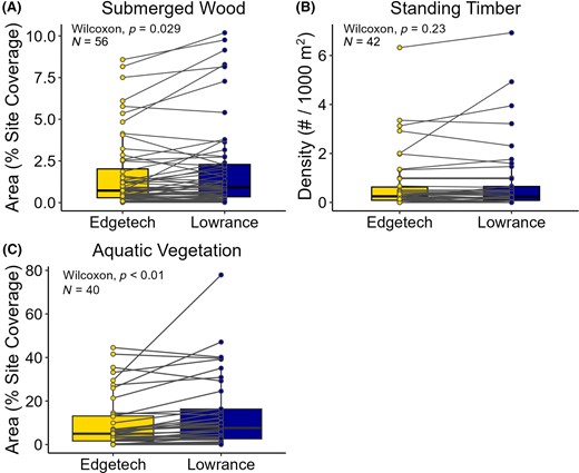
Comparisons of habitat values generated from the EdgeTech 6205 and Lowrance Active Imaging 3‐in‐1 side‐scan sonar imagery: (A) submerged woody debris, (B) standing timber, and (C) aquatic vegetation. Points connected by lines are paired values from a single Inland Management System sampling site.
In the shoreline‐to‐15‐m zone, mean areal estimates from the Lowrance imagery were significantly higher than those from the EdgeTech imagery (mean pairwise difference = 0.53%; Z = 2.819, p < 0.01), but no significant difference in areal estimates was observed in the 15–30‐m zone (Z = 0.779, p = 0.44; Figure S3). The two sets of sonar imagery did not vary significantly in terms of the number of polygons drawn in the shoreline‐to‐15‐m zone (Z = 1.202, p = 0.23; Figure S4). However, when we compared the areal size of 86 pairs of corresponding polygons (i.e., polygons delineating the same piece of wood in each set of imagery) in the shoreline‐to‐15‐m zone, polygons from the Lowrance imagery were significantly larger than those from the EdgeTech imagery (mean pairwise difference = 1.7 m2; Z = 5.757, p < 0.01; Figure S3 and Figure 3). Overall, areal estimates of submerged woody debris had a positive linear relationship, but we rejected the null hypothesis that areal estimates were equal between the two sonar systems (R2 = 0.89, p < 0.01; Figure S5).
Standing timber density estimates from the Lowrance imagery were not significantly different than those from the EdgeTech imagery (Z = 1.201, p = 0.23, N = 42 sites; Figure 2B; Figure S2B). The mean standing timber density from the Lowrance imagery was 0.8 ± 0.2 (mean ± SE) pieces per 1000 m2, whereas the mean standing timber density from the EdgeTech imagery was 0.7 ± 0.2 pieces per 1000 m2. Overall, standing timber density estimates from both sonar systems had a positive linear relationship, but we rejected the null hypothesis that densities were equal between the sonar systems (R2 = 0.89, p < 0.01; Figure S6).
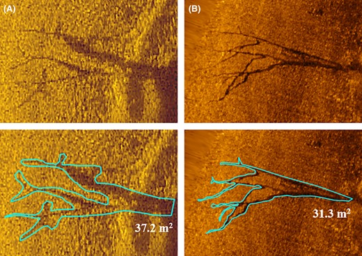
Comparison of woody debris appearance and polygon size in the 0–15‐m zone from the (A) Lowrance Active Imaging 3‐in‐1 side‐scan sonar imagery (polygon size = 37.2 m2) and (B) EdgeTech 6205 side‐scan sonar imagery (polygon size = 31.3 m2). (Scale = 1:200).
Vegetation value comparisons
Areal estimates of aquatic vegetation derived from the Lowrance imagery were significantly higher than those derived from the EdgeTech imagery (Z = 4.550, p < 0.01, N = 40 sites; Figure 2C; Figure S2C). The mean areal coverage of aquatic vegetation from the Lowrance imagery was 13.8 ± 2.7% (mean ± SE), whereas the mean areal coverage from the EdgeTech imagery was 9.8 ± 2.0%. This difference amounts to approximately 617 m2 of aquatic vegetation per site. Only 40 of the 56 total IMS sites were used for the vegetation metric comparison because no vegetation was observed in the remaining 16 sites. Overall, there was a positive correlation between aquatic vegetation areal coverage estimates from the two sonars, but we rejected the null hypothesis that areal estimates were equal between the sonar systems (R2 = 0.75, p < 0.01; Figure 4).

Linear relationship between aquatic vegetation areal estimates from the EdgeTech 6205 and Lowrance Active Imaging 3‐in‐1 side‐scan sonar imagery using major axis regression. The thick line is the linear fit, the thin lines represent the upper and lower 95% confidence limits, and the dotted line represents the null hypothesis that the slope is equal to 1.0. IMS, Inland Management System.
Substrate value comparisons
Mean IMS site‐level substrate composition estimates derived from the Lowrance and EdgeTech imagery were not significantly different (χ2 = 0.564, df = 5, p = 0.990, N = 38 sites; Figure 5; Figure S7). For each specific substrate type, the percent coverage estimates derived from the two sets of sonar imagery were within less than 3%. For the broad substrate categories, percent coverage estimates of “coarse” and “fine” substrates were within less than 1.5% for both sets of imagery. The EdgeTech imagery had more unclassified area per IMS site than the Lowrance imagery, with a mean difference of about 2.5%. Lastly, both sets of imagery had equal estimates (0.1%) of area classified as “other” (i.e., artificial structures) within the littoral area.
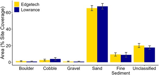
Comparison of mean site‐level benthic substrate composition values (±SE) generated from the EdgeTech 6205 and Lowrance Active Imaging 3‐in‐1 side‐scan sonar imagery (N = 38 Inland Management System sampling sites). The “other” category is excluded from this plot (areal proportion was ≈0.1% for both sonar systems).
Vegetation ground‐truthing accuracy
EdgeTech imagery was only available for early spring of 2022, prior to any significant vegetation growth, so the relationship between vegetation ground‐truthing and side‐scan data could only be assessed for the Lowrance imagery. All accuracy comparisons are based on classification by a single researcher (T. Fletcher). Total accuracy for aquatic vegetation mapping was approximately 90.2%, with 1041 of the 1154 ground truth points falling within a correctly classified area (Table 1). Accuracy was highest in sites with no vegetation present (score = 0; 766 of 828 points; ≈92.5%), areas of moderate vegetation density (score = 2; 37 of 38 points; ≈97.4%), and areas of high vegetation density (score = 3; 26 of 27 points; ≈96.3%). Accuracy was lowest in areas with low vegetation density (score = 1; 130 of 170 points; ≈76.5%). Areas with emergent vegetation were typically classified correctly (lily pads: 7 of 8 points, 87.5%; American water willow: 75 of 83 points, ≈90.4%). Overall classifications were significantly better than random ( = 0.76, variance = 0.0005, Z = 35.85). However, classification performance varied among the reservoirs (Table S1), with highest accuracy at Acton Lake ( = 0.84, variance = 0.001, Z = 24) and similar values at Rocky Fork Lake ( = 0.64, variance = 0.001, Z = 16.12) and Caesar Creek Lake ( = 0.63, variance = 0.004, Z = 9.52). The majority of misclassifications were at low vegetation density.
Vegetation classification accuracy results for the Lowrance Active Imaging 3‐in‐1 side‐scan sonar imagery. Scored ground truth points were overlaid on vegetation polygons within a geographical information system to determine whether presence/absence was accurately classified within the GIS vegetation layer. Numbers highlighted in gray shading indicate correct classifications.
| Classified data and producer's accuracy | Reference data | |||||||
| 0 (no vegetation) | 1 (low) | 2 (moderate) | 3 (high) | Lily pads | American water willow | Row total | User's accuracy (%) | |
| No vegetation | 766 | 40 | 1 | 1 | 1 | 8 | 817 | 94.0 |
| Vegetated | 62 | 130 | 37 | 26 | 7 | 75 | 337 | 82.0 |
| Column total | 828 | 170 | 38 | 27 | 8 | 83 | 1154 | |
| Producer's accuracy (%) | 92.5 | 76.5 | 97.4 | 96.3 | 87.5 | 90.4 | 90.2 (overall accuracy) | |
Among all three reservoirs, there was a total of 113 ground‐truthing points that were located at misclassified areas. Of these 113 points, 62 were false‐positive classifications (i.e., vegetation was not present and ground truth score = 0, but vegetation was classified on side‐scan imagery). To account for potential inaccuracy in the location of side‐scan imagery, we estimated the distance between each ground truth point at a misclassified location and the nearest vegetation polygon. We determined that 47 (≈75.8%) of these 62 false‐positive misclassifications were within 5 m of a matching zone (i.e., area with no vegetation polygon), 37 (≈59.7%) were within 3 m, and 17 (≈27.4%) were within 1 m. The remaining 51 points that were located at a misclassified area were false‐negative classifications (vegetation was present and ground truth score = 1–3, but vegetation was not identified in the imagery). Of these 51 false‐negative misclassifications, 27 (≈52.9%) were within 5 m of a matching zone (i.e., a vegetation polygon), 18 (≈35.3%) were within 3 m, and 9 (≈17.6%) were within 1 m.
Substrate ground‐truthing accuracy
We used a total of 1573 ground‐truthing points to determine accuracy rates for the manual substrate classification process. All accuracy comparisons are based on classification by a single researcher (T. Fletcher). In the Lowrance imagery, 175 of these 1573 points fell within an area labeled as “unclassified” and the remaining 1398 points fell within classified substrate polygons. Of the 1398 classified ground‐truthing points, 900 were recorded as having only a single substrate type present. Multiple substrates were recorded at the remaining 498 points. In the EdgeTech imagery, 252 of 1573 points fell within an area labeled as “unclassified” and the remaining 1321 points fell within classified substrate polygons. Of the 1321 classified ground truth points, 861 were recorded as having only a single substrate type present. Multiple substrates were recorded at the remaining 460 points.
Under the manual classification scheme for specific substrate types (i.e., boulder, cobble, gravel, sand, and fines; Table 2), 687 (≈76.3%) of 900 single‐substrate points were correctly classified in the Lowrance imagery. In the EdgeTech imagery, 667 (≈77.5%) of 861 single‐substrate points were correctly classified. For both sets of imagery, points containing sand had the highest classification accuracy (Lowrance: 90.9%; EdgeTech: 92.6%), whereas points containing gravel had the lowest classification accuracy (Lowrance and EdgeTech: 0.0%). Overall classifications were significantly better than random for both sonar systems (EdgeTech: = 0.425, variance = 0.001, Z = 13.23; Lowrance: = 0.403, variance = 0.001, Z = 12.72). Classification performance between sonar types did not differ significantly among the study lakes (Table S2; Acton Lake: Z = 0.592, Rocky Fork Lake: Z = 0.567, Caesar Creek Lake: Z = 0.465). However, classification performance was greater for both sonars at Acton Lake than at either Rocky Fork Lake (EdgeTech: Z = 4.03; Lowrance: Z = 3.36) or Caesar Creek Lake (EdgeTech: Z = 3.36; Lowrance: Z = 2.34).
Manual substrate classification results using single‐substrate ground‐truthing points for the EdgeTech 6205 and Lowrance Active Imaging 3‐in‐1 (AI31) side‐scan sonar imagery. Ground truth points were overlaid on manually drawn substrate polygons. Numbers highlighted in gray shading indicate correct classifications.
| Classified data and producer's accuracy | Reference data | ||||||
| Boulder | Cobble | Gravel | Sand | Fines | Row total | User's accuracy (%) | |
| Edgetech 6205 | |||||||
| Boulder | 4 | 0 | 0 | 5 | 1 | 10 | 40.0 |
| Cobble | 1 | 6 | 2 | 4 | 1 | 14 | 42.9 |
| Gravel | 0 | 0 | 0 | 5 | 3 | 8 | 0.0 |
| Sand | 3 | 5 | 19 | 560 | 111 | 698 | 80.2 |
| Fines | 3 | 0 | 0 | 31 | 97 | 131 | 74.0 |
| Column total | 11 | 11 | 21 | 605 | 213 | 861 | |
| Producer's accuracy (%) | 36.4 | 54.5 | 0.0 | 92.6 | 45.5 | 77.5 (overall accuracy) | |
| Lowrance AI31 | |||||||
| Boulder | 8 | 5 | 0 | 5 | 0 | 18 | 44.4 |
| Cobble | 0 | 7 | 0 | 6 | 0 | 13 | 53.8 |
| Gravel | 0 | 3 | 0 | 17 | 0 | 20 | 0.0 |
| Sand | 2 | 10 | 4 | 579 | 42 | 637 | 90.9 |
| Fines | 2 | 1 | 2 | 114 | 93 | 212 | 43.9 |
| Column total | 12 | 26 | 6 | 721 | 135 | 900 | |
| Producer's accuracy (%) | 66.7 | 26.9 | 0.0 | 80.3 | 68.9 | 76.3 (overall accuracy) | |
Under the manual classification scheme for broad substrate categories, total classification accuracy was comparable for both the Lowrance (96.8%) and EdgeTech (96.9%) side‐scan data (Table 3). A vast majority (>88.5%) of the ground truth points contained only “fine” substrates, and the classification accuracy for these points was slightly higher with the EdgeTech system (98.3%) than with the Lowrance system (97.8%). For both sets of imagery, a small proportion (<4.0%) of ground truth points contained only “coarse” substrates. The classification accuracy for these “coarse” substrate points was higher with the Lowrance system (72.5%) than with the EdgeTech system (43.8%). Overall classifications were significantly better than random for both sonar systems (Table S3; EdgeTech: = 0.408, variance = 0.006, Z = 5.25; Lowrance: = 0.627, variance = 0.003, Z = 11.67). Classification performance between sonar types differed significantly only for Caesar Creek Lake (Z = 2.18; Acton Lake: Z = 1.54; Rocky Fork Lake: Z = 0.49), primarily due to misclassification of coarse sediments. Classification performance was greater for EdgeTech at Acton Lake than at Caesar Creek Lake (Z = 3.49) and was greater for Lowrance at Acton Lake than at Rocky Fork Lake (Z = 4.12). Moreover, for both the Lowrance and EdgeTech imagery, ground truth points containing only “coarse” substrates were 2.5 times more likely to fall within an area labeled as “unclassified” than ground truth points containing only “fine” substrates (Figure S1; Table 4).
Manual substrate classification results for broad (i.e., “coarse” vs. “fine”) classification scheme substrate types for the EdgeTech 6205 and Lowrance Active Imaging 3‐in‐1 (AI31) side‐scan sonar imagery. Ground truth points were overlaid on manually drawn substrate polygons. Numbers highlighted in gray shading indicate correct classifications.
| Classified data and producer's accuracy | Reference data | |||||||||||
| Boulder | Cobble | Boulder/cobble | Gravel | Sand | Fine sediment | Gravel/sand | Gravel/fine sediment | Sand/fine sediment | Gravel/sand/fine sediment | Row total | User's accuracy (%) | |
| Edgetech 6205 | ||||||||||||
| Coarse | 5 | 6 | 3 | 2 | 9 | 2 | 7 | 0 | 0 | 0 | 34 | 41.2 |
| Fine | 6 | 5 | 7 | 19 | 596 | 211 | 153 | 4 | 181 | 13 | 1195 | 98.5 |
| Column total | 11 | 11 | 10 | 21 | 605 | 213 | 160 | 4 | 181 | 13 | 1229 | |
| Producer's accuracy (%) | 45.5 | 54.5 | 30.0 | 90.5 | 98.5 | 99.1 | 95.6 | 100 | 100 | 100 | 96.9 (overall accuracy) | |
| Lowrance AI31 | ||||||||||||
| Coarse | 13 | 7 | 17 | 3 | 12 | 3 | 6 | 1 | 2 | 0 | 64 | 57.8 |
| Fine | 5 | 6 | 3 | 17 | 625 | 209 | 163 | 2 | 187 | 13 | 1230 | 98.9 |
| Column total | 18 | 13 | 20 | 20 | 637 | 212 | 169 | 3 | 189 | 13 | 1294 | |
| Producer's accuracy (%) | 72.2 | 53.8 | 85.0 | 85.0 | 98.1 | 98.6 | 96.4 | 66.7 | 98.9 | 100 | 96.8 (overall accuracy) | |
Manual substrate classification results depicting the proportion of unclassified “coarse” and “fine” ground truth points from the EdgeTech 6205 and Lowrance Active Imaging 3‐in‐1 (AI31) side‐scan sonar imagery.
| Ground truth points | Total number | EdgeTech unclassified | Lowrance AI31 unclassified |
| Points with only coarse substrates | 70 | 38 (54.3%) | 19 (27.1%) |
| Points with only fine substrates | 1375 | 178 (12.9%) | 132 (9.6%) |
| Ground truth points | Total number | EdgeTech unclassified | Lowrance AI31 unclassified |
| Points with only coarse substrates | 70 | 38 (54.3%) | 19 (27.1%) |
| Points with only fine substrates | 1375 | 178 (12.9%) | 132 (9.6%) |
Comparisons of GIS processing time
Overall, GIS processing of the different habitat types generally took longer with the EdgeTech imagery than with the Lowrance imagery (Table 5). The GIS processing of submerged woody debris took significantly longer with the EdgeTech imagery than it did with the Lowrance imagery (mean pairwise difference = 3.3 min/site; Z = 3.509, p < 0.01, N = 24 sites). Significantly more woody debris polygons were drawn using the EdgeTech imagery (mean pairwise difference = 10.5 polygons/site; Z = 2.647, p < 0.01). The GIS processing of vegetation also took significantly longer with the EdgeTech imagery than it did with the Lowrance imagery (mean pairwise difference = 0.9 min/site; Z = 2.980, p < 0.01, N = 24 sites). Similarly, GIS processing of benthic substrate also took significantly longer with the EdgeTech imagery (mean pairwise difference = 0.9 min/site; Z = 2.885, p < 0.01, N = 24 sites). However, there was no significant difference in the number of polygons drawn from each set of imagery for vegetation (EdgeTech: 4.0 ± 0.7 polygons/site; Lowrance: 5.0 ± 0.7 polygons/site; Z = 1.798, p = 0.072) or benthic substrate (EdgeTech: 9.1 ± 1.0 polygons/site; Lowrance: 7.7 ± 0.7 polygons/site; Z = 1.419, p = 0.16). Lastly, GIS processing times for standing timber were similar between the two sets of sonar imagery (EdgeTech: 2.6 ± 0.7 min/site; Lowrance: 2.7 ± 0.7 min/site; Z = 0.542, p = 0.59, N = 16 sites).
Processing time comparison for all habitat types from the EdgeTech 6205 and Lowrance Active Imaging 3‐in‐1 side‐scan sonar imagery. Processing time (mean ± SE) is given in minutes per Inland Management System (IMS) site. Values in bold are statistically significant (α = 0.05).
| Habitat type | Lowrance processing time (min/IMS site) | EdgeTech processing time (min/IMS site) | Z | p |
| Submerged woody debris | 12.7 ± 1.6 | 16.0 ± 2.4 | 3.509 | <0.01 |
| Aquatic vegetation | 5.8 ± 0.6 | 6.7 ± 0.7 | 2.980 | <0.01 |
| Substrate | 8.5 ± 0.2 | 9.4 ± 0.4 | 2.885 | <0.01 |
| Standing timber | 2.7 ± 0.7 | 2.6 ± 0.7 | 0.542 | 0.59 |
Analyst variation/bias in GIS processing
The magnitude of analyst bias in GIS processing varied among habitat types (Table 6). Specifically, our analysis of GIS analyst bias for both sets of sonar imagery revealed that analyst identity had no significant influence on submerged woody debris (Lowrance: F2, 39 = 0.116, p = 0.891; EdgeTech: F2, 39 = 0.088, p = 0.916) or aquatic vegetation (Lowrance: F2, 39 = 1.267, p = 0.293; EdgeTech: F2, 39 = 0.584, p = 0.562) habitat estimates. However, analyst identity did have a significant influence on benthic substrate habitat values that were derived from the EdgeTech imagery. Specifically, analyst identity significantly impacted both “coarse” (F2, 39 = 4.071, p = 0.025) and “fine” (F2, 39 = 6.247, p < 0.01) substrate estimates from the EdgeTech imagery. These differences were primarily attributable to significant variation in estimates of both cobble (F2, 39 = 4.34, p = 0.02) and sand (F2, 39 = 4.168, p = 0.023). Analyst identity had no influence on “coarse” (F2, 39 = 0.324, p = 0.725) or “fine” (F2, 39 = 0.386, p = 0.682) substrate estimates derived from the Lowrance imagery, and no significant difference in estimates among analysts was observed for any specific substrate type.
One‐way analysis of variance results of analyst bias (N = 3 analysts) from habitat classification at Acton Lake (N = 14 Inland Management System [IMS] sampling sites), Ohio, using the EdgeTech 6205 and Lowrance Active Imaging 3‐in‐1 (AI31) side‐scan sonar imagery. Values in bold are statistically significant (α = 0.05).
| Sonar and habitat type | Range of analyst means (%; per IMS site) | F | p |
| Lowrance AI31 | |||
| Submerged woody debris | 3.47–4.13 | 0.116 | 0.891 |
| Aquatic vegetation | 6.63–8.80 | 1.267 | 0.293 |
| Coarse substrate | 6.79–10.68 | 0.324 | 0.725 |
| Boulder | 0.57–1.58 | 0.430 | 0.653 |
| Cobble | 5.66–9.69 | 0.368 | 0.695 |
| Fine substrate | 75.14–80.63 | 0.386 | 0.682 |
| Gravel | 0.00–2.95 | 1.162 | 0.323 |
| Sand | 63.89–70.82 | 0.557 | 0.577 |
| Fine sediment | 1.37–10.62 | 3.003 | 0.06 |
| EdgeTech 6205 | |||
| Submerged woody debris | 2.87–3.33 | 0.088 | 0.916 |
| Aquatic vegetation | 3.43–4.25 | 0.584 | 0.562 |
| Coarse substrate | 5.98–18.71 | 4.071 | 0.025 |
| Boulder | 0.43–1.16 | 0.38 | 0.686 |
| Cobble | 4.82–18.27 | 4.340 | 0.02 |
| Fine substrate | 63.69–81.28 | 6.247 | <0.01 |
| Gravel | 0.00–0.25 | 3.011 | 0.06 |
| Sand | 47.02–67.75 | 4.168 | 0.023 |
| Fine sediment | 11.92–20.00 | 2.087 | 0.138 |
DISCUSSION
In this study, we used both recreational (Lowrance) and survey‐grade (EdgeTech) side‐scan sonar imagery to manually quantify submerged woody debris, standing timber, aquatic vegetation, and benthic substrate in the littoral zone within three highly eutrophic Ohio reservoirs. Despite substantial differences in image resolution, clarity, and contrast, we were generally able to quantify habitat features in the imagery from both sonar systems at the scale of 500‐m IMS sampling sites, with broadly similar results. However, through this comparison, we found trade‐offs between recreational and survey‐grade sonar units. Data acquisition, data processing, and habitat mapping were more time‐intensive with the EdgeTech imagery than with the Lowrance imagery. Moreover, despite (or due to) the high resolution of the EdgeTech imagery, separate GIS analysts had greater variation in delineating substrate. The Lowrance sonar unit was able to capture imagery closer to the shoreline and was less impacted by the presence of dense aquatic vegetation than the EdgeTech sonar. However, the relatively low‐resolution imagery from the Lowrance unit contained higher levels of distortion and overestimated the area of certain habitat types within the littoral zone. Ultimately, although survey‐grade sonar systems like the EdgeTech provide high‐quality imagery with increased positional accuracy, our data indicate that for habitat assessment in the littoral zones of reservoirs, recreational sonar units such as the Lowrance sonar can provide similar data with lower investments in equipment and time.
After classifying individual habitat types across the three study reservoirs, we found that habitat values derived from both sonar systems' imagery were generally similar. For woody habitat, no difference in standing timber density estimates was observed. However, imagery from the Lowrance unit did produce significantly higher estimates of submerged woody debris than the EdgeTech imagery. Further analyses revealed that this was primarily attributable to larger woody debris polygon sizes in the nearshore (0–15‐m) area for the Lowrance imagery. It is well understood that sonar signals suffer distortion from numerous sources during transmission, propagation, and reception (Bjørnø 2017). Moreover, distortion on side‐scan imagery is more frequently observed at longer ranges and lower frequencies (Cobra et al. 1992). Fleming et al. (2018) noted that recreational side‐scan units generally operate at lower frequencies than survey‐grade systems and produce lower resolution imagery. In this case, the lower transmission frequency of the Lowrance system (455 kHz) relative to the EdgeTech system (550 kHz) likely caused higher levels of distortion in the nearshore areas of the imagery that were furthest from the boat path. This distortion made pieces of submerged woody debris appear larger and with less defined edges on the Lowrance imagery, which likely resulted in an overestimate of the areal coverage of submerged woody debris in the littoral zone. However, it should be noted that site‐level estimates of submerged woody debris from both sonars were strongly related, and an exact measurement of the amount of woody debris is likely to be less important than a relative estimate for most ecological applications. Accordingly, this result further highlights the ability of side‐scan sonar to accurately map and quantify the presence of woody debris in freshwater environments (Kaeser and Litts 2008; Kitchingman et al. 2013; Daugherty et al. 2015). Due to visibility constraints, we were unable to assess classification accuracy for the submerged woody debris and standing timber habitats. Given the discrete and conspicuous appearance of both submerged woody debris and standing timber on side‐scan imagery, it is unlikely that such features were misidentified, but their exact dimensions may be inaccurate.
The Lowrance imagery also produced significantly higher estimates of aquatic vegetation than the EdgeTech imagery. Although some of this variation may be attributable to the same distortion that caused the disparity in areal woody debris estimates, the relative ability of each sonar system to penetrate through areas of dense vegetation and capture imagery up to the shoreline appears to be the primary driver of this difference in aquatic vegetation estimates (Figure S8). Fleming et al. (2018) noted that survey‐grade sonar systems are relatively large devices, which have several limitations that restrict their use as a survey tool in many freshwater environments. Recreational sonar units, on the other hand, are smaller in size and can be more easily deployed in shallow lakes and rivers (Halmai et al. 2020). Due to the high turbidity and eutrophic nature of the sampled reservoirs, vegetation was generally only present in shallow littoral areas. In areas of minimal to moderate vegetation growth, the two sonar systems provided similar estimates of areal vegetation coverage. However, in zones of dense, expansive vegetation, the Lowrance system was generally able to obtain imagery closer to the shoreline edge than the EdgeTech system, resulting in larger, more accurate areal vegetation estimates. These results, along with our relatively high rate of classification accuracy (90.2%), corroborate the findings of past studies that emphasized the utility of recreational side‐scan sonar in mapping aquatic vegetation (Daugherty et al. 2015; Greene et al. 2018; Bennett et al. 2020).
Mean site‐level estimates of benthic substrate composition were also comparable between the two sonar systems. Specifically, mean values for each substrate type derived from the Lowrance imagery were within less than 3% of those derived from the EdgeTech imagery. To our knowledge, only one prior study (Hamill et al. 2018) has directly compared proportional substrate estimates derived from recreational and survey‐grade sonar data. In that study, automated substrate classification was performed using recreational side‐scan imagery, and estimated reach‐scale proportions of sand, gravel, and boulder were likewise found to be within 3% of estimates derived from survey‐grade multibeam sonar maps. Our manual substrate classification accuracy was also similar between the two sonar systems. Accurate classification of substrates from side‐scan imagery has been historically challenging, and reported accuracy rates from individual studies have varied widely (Graham et al. 2017). For example, Walker and Alford (2016) attempted to map Lake Sturgeon spawning habitat in the upper Tennessee River and reported substrate classification accuracy rates between 29% and 33% using eight individual substrate classes. Conversely, Richter et al. (2016) sought to map Walleye Sander vitreus spawning substrates in a group of northern Wisconsin lakes and reported a classification accuracy rate of 93% using six individual substrate classes. In our project, both sonar systems had similar performance: under the specific classification scheme (six substrate classes), overall classification accuracy was between 76% and 78%, while under the broad classification scheme (coarse vs. fine), accuracy was between 96% and 97%. Ultimately, substrate classification accuracy with side‐scan sonar imagery will depend heavily on the total number of substrate classes being used. Fewer and broader classes will generally produce higher accuracy rates (Walker and Alford 2016). However, the number and type of classes selected also need to be relevant to the desired biological objectives. Therefore, a balance between classification accuracy, substrate data resolution, and the number of dominant substrate types present is always an important consideration when determining the appropriate number of substrate classes.
It should be noted that the reservoirs sampled as part of this study have a relatively simple substrate structure, with a significant majority of the benthic zone being composed of sand and fine sediment. Larger substrates, such as boulder and cobble, are generally rare in these reservoirs and tend to be concentrated in shallow areas close to the shoreline (Daugherty et al. 2015). The asymmetric presence of fine‐grain substrates in our sampled reservoirs not only resulted in relatively high rates of classification accuracy for “fine” substrate types (97.8–98.3% under the broad classification scheme) but also disproportionately increased the overall classification accuracy rates. Indeed, classification accuracy for “coarse” substrates was substantially lower than the overall accuracy rates (Lowrance: 72.5%; EdgeTech: 43.8%). Richter et al. (2016) likewise found that despite a relatively high classification accuracy rate of 93%, a substantial percentage of their substrate misclassifications occurred among coarse substrates. This discrepancy in coarse‐substrate classification accuracy was ultimately attributed to embeddedness (Richter et al. 2016). Embeddedness occurs when coarse substrates are heavily surrounded by sand and fine sediment, which causes coarse substrates to have a more smooth and uniform appearance on side‐scan imagery (Richter et al. 2016). This may ultimately result in coarse substrates being misclassified as a finer sediment type (Richter et al. 2016). In our case, the overwhelming presence of sand and fine‐sediment substrates appears to have resulted in some degree of embeddedness, which ultimately reduced classification accuracy for larger substrates, such as boulder, cobble, and gravel. Compared to other rocky substrates, gravel is especially vulnerable to misclassification when surrounded by sand due to its relatively small grain size (0.02–0.064 m) relative to side‐scan pixel width (0.05–0.075 m in this study), which often results in a more uniform appearance on side‐scan imagery (Kaeser and Litts 2010; Richter et al. 2016). Indeed, gravel was never correctly classified in our sonar imagery (i.e., accuracy = 0%) and was most frequently classified as sand (85% of the time).
In addition to habitat quantities and classification accuracy, we also compared the relative efficiency of data acquisition, data processing, and habitat classification between the EdgeTech and Lowrance sonar systems. Overall, data acquisition with the EdgeTech system was 6–10× more time‐intensive than it was with the Lowrance system in both field data collection and postprocessing. Although the process of collecting side‐scan data (i.e., driving the boat around the perimeter of the lake at relatively low speed) was generally the same for both sonars, the large size of the EdgeTech sonar head made it more vulnerable to collisions with underwater obstructions, such as standing timber. These findings are consistent with prior studies, which have noted that survey‐grade sonar systems like the EdgeTech sonar are of limited use in shallow environments due to their relatively large size (Fleming et al. 2018; Halmai et al. 2020) as well as the significant costs, operational complexities, and additional time and expertise required for data processing and analysis (Tian 2011).
We expected that the improved quality of survey‐grade imagery would result in greater consistency among analysts when manually delineating habitat. Instead, we found greater variation in substrate habitat values generated by separate GIS analysts from EdgeTech imagery, particularly in estimates of sand and cobble substrates. In contrast, there was no significant difference among the habitat values generated by different analysts with the Lowrance imagery. Compared to recreational sonar systems, the higher signal‐to‐noise ratio of survey‐grade systems like the EdgeTech gives them a superior ability to resolve and capture imagery of features and objects in the path of the sonar beam (Fleming et al. 2018). This seems to have resulted in more detail and textural heterogeneity appearing in the image, which ultimately resulted in greater differences of opinion among the individual interpreters regarding the benthic substrate composition. Conversely, the relatively low level of detail in the Lowrance imagery likely resulted in a more uniform appearance, which reduced the amount of interpretive bias among GIS analysts in the manual substrate classification process (but does not necessarily improve classification accuracy). However, variation in GIS analyst experience with side‐scan imagery is also an important factor to consider. Among the analysts in our project, only one had extensive experience in the interpretation of side‐scan imagery. Less experienced users seem likely to have less internal and among‐user consistency, which is magnified by the more detailed EdgeTech imagery because more potential features may be visible. It is possible that this interpretive bias would have been reduced (and classification accuracy would have increased) if all analysts had similar and higher levels of experience. The among‐user variation observed highlights the need for shared reference libraries and co‐training on delineation with a subset of imagery to maximize among‐user consistency, similar to approaches with other visual methods employed in fisheries (e.g., otoliths).
Our goal in this study was to compare the performance of the EdgeTech and Lowrance sonar systems by quantifying habitat features in the littoral zones of reservoirs. We focused our efforts on littoral areas because of the biological importance of littoral habitats for sport fish (Daugherty et al. 2015; Richter et al. 2016). However, because our study design focuses only on littoral areas at the spatial scale of the IMS site, it fails to highlight some of the major advantages associated with survey‐grade sonar—namely, accurate positioning, a high signal‐to‐noise ratio, and the ability to collect swath bathymetry concurrently with side‐scan imagery. Since our zone of interest could be completely captured within a single swath width (100 m), the limited spatial accuracy of the recreational sonar primarily means that the imagery is unlikely to represent the exact position of habitat features and, to some extent, their size. Therefore, understanding fish associations with specific habitat features, which is often an objective of telemetry projects, could be difficult when using recreational‐grade sonars. In areas of swath overlap, habitat features are likely to be misaligned or duplicated on the processed imagery collected using a recreational sonar. The high spatial accuracy (<10 cm) of survey‐grade sonar data allows accurate mosaicking of overlapping swaths of imagery. In addition, within deeper, offshore areas, the higher power and signal‐to‐noise ratio of the EdgeTech system provide more consistent image quality, which is particularly relevant when a larger portion of the side‐scan swath is occupied by the water column. Our study approach did not incorporate the EdgeTech system's high‐resolution, multi‐beam bathymetry, which can be used to correct the brightness of side‐scan imagery for depth—a potentially useful feature for classifying substrate.
Although beyond the scope of our project, clearly there are promise and interest in automating the classification of habitat from side‐scan imagery (Buscombe et al. 2016; Hamill et al. 2016, 2018; Buscombe 2017; Bodine et al. 2022), and future work should investigate the potential trade‐offs in image classification between recreational and survey‐grade side‐scan data, where more detailed imagery may facilitate the achievement of high classification accuracy from algorithmic approaches. Ultimately, we believe that recreational side‐scan sonar systems such as the Lowrance system are an efficient and practical solution for mapping littoral habitat features in reservoir environments. Given the context of our interest in littoral zone habitat, the shortcomings of the recreational system were minimal and its ease of use and ability to record imagery for shallow nearshore regions were evident. Moreover, we observed little difference in habitat classification values and accuracy between the two types of sonar systems, and processing times and interpreter variation were minimized with the Lowrance imagery. These factors, combined with the enormous reduction in cost, make recreational side‐scan sonar systems a useful tool for littoral habitat surveying in reservoirs.
ACKNOWLEDGMENTS
Financial support for this research was provided by the Federal Aid in Sport Fish Restoration Program (F‐69‐P; Fish Management in Ohio), administered jointly by the U.S. Fish and Wildlife Service and the Ohio Department of Natural Resources–Division of Wildlife as State Project FADR85. We thank Rob Tewes and Ryan Argo (Ohio River Valley Water Sanitation Commission) for their assistance with the ground‐truthing process. We also appreciate Lisa Wolfe (Echo 81 LLC) for her help with the training and rental of the EdgeTech 6205 sonar system. Lastly, we thank all individuals within the University of Cincinnati's Department of Biological Sciences that assisted with data collection, data processing, and other portions of the study.
CONFLICT OF INTEREST STATEMENT
Although this study used particular brands and models of equipment in comparing sonar technology for use in mapping habitat, the mention of these specific products or brands does not constitute endorsement by the authors or their agencies. None of the authors has any personal, professional, or financial affiliation with the companies whose equipment was used in this study, all equipment was purchased or rented for the study, and the contents of the manuscript were not discussed with outside entities.
DATA AVAILABILITY STATEMENT
Data are available from the Environmental Data Initiative data repository: https://doi.org/10.6073/pasta/85b5702b786c05ffbe4263dfd755663f.
ETHICS STATEMENT
There were no ethical guidelines applicable to this study.
