


Abstract
To comply with legal mandates, meet local management objectives, or both, many federal, state, and tribal organizations have monitoring groups that assess stream habitat at different scales. This myriad of groups has difficulty sharing data and scaling up stream habitat assessments to regional or national levels because of differences in their goals and data collection methods. To assess the performance of and potential for data sharing among monitoring groups, we compared measurements made by seven monitoring groups in 12 stream reaches in northeastern Oregon. We evaluated (1) the consistency (repeatability) of the measurements within each group, (2) the ability of the measurements to reveal environmental heterogeneity, (3) the compatibility of the measurements among monitoring groups, and (4) the relationships of the measurements to values determined from more intensive sampling (detailed measurements used as a standard for accuracy and precision in this study). Overall, we found that some stream attributes were consistently measured both within and among groups. Furthermore, for all but one group there was a moderate correlation (0.50) between the group measurements and the intensive values for at least 50% of the channel attributes. However, none of the monitoring groups were able to achieve high consistency for all measured stream attributes, and few of the measured attributes had the potential for being shared among all groups. Given the high cost of stream habitat monitoring, we suggest directing more effort to developing approaches that will increase the consistency and compatibility of measured stream attributes so that they will have broader utility. Ultimately, local monitoring programs should consider incorporating regional and national objectives so that data can be scaled up and the returns to limited monitoring dollars can be maximized across spatial scales.
To meet management objectives and respond to environmental laws and regulations, many state, federal, and tribal agencies monitor the status and trend of stream habitat (Johnson et al. 2001; Whitacre et al. 2007). Physical characteristics of stream habitat are often monitored as a cost‐effective surrogate for direct assessments of biological condition (Fausch et al. 1988; Budy and Schaller 2007). These data can also be used to assess watershed condition (Buffington et al. 2003) and degree of landscape disturbance (Woodsmith and Buffington 1996; Kershner et al. 2004). Understanding current stream conditions and how they change through time can be a critical first step to better understanding cause‐and‐effect relationships between measured stream attributes and the environmental processes that form and alter them. For example, evaluation of historic and long‐term monitoring data has resulted in a better understanding of the effects of timber harvest on stream habitat and salmonid production in western North America (McIntosh et al. 1994; Hartman et al. 1996; Isaak and Thurow 2006; Smokorowski and Pratt 2007; Honea et al. 2009). Determining these cause‐and‐effect relationships is often recognized as a key factor for improving management of stream systems and implementing successful restoration programs (Bilby et al. 2004).
Many aquatic monitoring groups collect data on the status and trend of stream habitat at mesoscales associated with group‐specific jurisdiction (e.g., state or management unit levels), but few collect data at broad enough scales and sufficient sampling intensity to evaluate regional or national conditions (Bernhardt et al. 2005; but see EPA 2006a for the exception). If data could be combined across multiple monitoring groups, it would enable larger‐scale assessments and greatly increase the statistical power of regional and national assessments (Urquhart et al. 1998; Larsen et al. 2007; Whitacre et al. 2007). Examples of national and regional assessments that could benefit from being able to combine data from different monitoring programs include the U.S. Environmental Protection Agency's (EPA) assessment of surface waters (EPA 2006a) and the National Oceanic and Atmospheric Administration's (NOAA) effort to monitor the recovery of salmon Oncorhynchus spp. and steelhead O. mykiss in the Pacific Northwest (Crawford and Rumsey 2009). Both of these assessments have general objectives of conducting “baseline status and trend monitoring” and would benefit from increased sample sizes and more widespread sampling.
A review of attributes measured by monitoring groups reveals a large number of commonly measured attributes (Johnson et al. 2001). However, combining data across disparate monitoring groups can be difficult because of differences in group objectives, site selection processes, methods for measuring specific stream attributes (both in general terms and specific details of how and where), and the amount and type of training that monitoring crews receive (Bonar and Hubert 2002; Whitacre et al. 2007). Even when monitoring groups have similar objectives and measure the same attributes, the measured values may be inherently different from one another because of the above differences. Nevertheless, the potential still exists to combine data across monitoring groups if the measurements within each group are consistent (repeatable) and are correlated to results from other groups. However, consistency and correlation do not guarantee accuracy of measurements, which also must be evaluated. Ideally, attribute measurements for status‐and‐trend monitoring should be consistent, precise, accurate, and capable of detecting environmental heterogeneity and change.
The goal of this paper is to assess the performance and compatibility of measurements obtained from seven monitoring groups that all use different monitoring protocols to assess stream habitat throughout the Pacific Northwest. This analysis expands on previous work defining acceptable levels of variability within stream habitat protocol data (Kaufmann et al. 1999; Whitacre et al. 2007). To address these issues, we examine (1) the consistency of the measurements within monitoring groups, (2) the ability of each monitoring protocol to detect environmental heterogeneity, (3) the compatibility of the measurements between monitoring groups, and (4) the relationships of the measurements to more intensive stream measurements that may better describe the true character of stream habitat (discussed further below). Understanding how the results of different monitoring programs are related to each other may foster improvement in the quality of stream habitat data, increase the sharing of data across monitoring groups, and increase statistical power to detect environmental trends (Larsen et al. 2007).
Study Sites
Data were collected from 12 streams in the John Day River basin in northeastern Oregon, which ranges in elevation from 80 m at the confluence with the Columbia River to over 2,754 m in the headwaters of the Strawberry Mountain Range (Figure 1; Table 1). This location was selected for several reasons: there was an ongoing collaborative agreement between different state and federal agencies in the state of Oregon; several of the groups had sample sites in the basins; and the logistics of organizing numerous groups were optimal (access, proximity of monitoring groups, and timing).
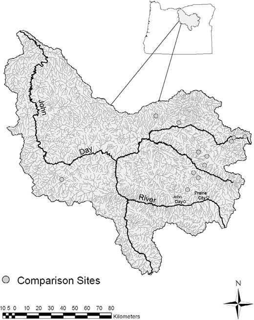
Locations of the study sites within the John Day River basin (modified from Roper et al. 2008).
Characteristics of the 12 streams sampled in the John Day basin. The values for gradient, bank‐full width (BFW), and the bank‐full width‐to‐depth ratio (W:D) are averages across all monitoring protocols and field crews. The values for sinuosity, residual pool depth (RPD), and median particle size (D50) are averages across all of the groups that collected these attributes. Large woody debris (LWD) is defined as pieces having a length of 3 m or more and a diameter of 0.1 m or more and includes data from four groups (AREMP, EMAP, PIBO, and ODFW; see text)
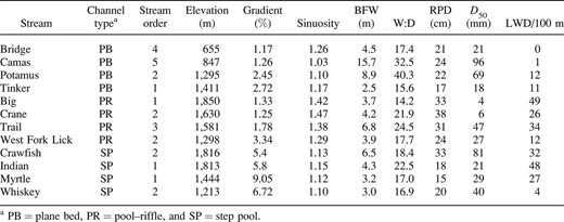
Characteristics of the 12 streams sampled in the John Day basin. The values for gradient, bank‐full width (BFW), and the bank‐full width‐to‐depth ratio (W:D) are averages across all monitoring protocols and field crews. The values for sinuosity, residual pool depth (RPD), and median particle size (D50) are averages across all of the groups that collected these attributes. Large woody debris (LWD) is defined as pieces having a length of 3 m or more and a diameter of 0.1 m or more and includes data from four groups (AREMP, EMAP, PIBO, and ODFW; see text)
The John Day basin is located within the Blue Mountains ecoregion (Clarke and Bryce 1997), which encompasses a wide range of climates (semiarid to subalpine) and vegetation types (grassland, sagebrush [Artemisia spp.], and juniper [Juniperus spp.] at lower elevations to mixed fir [Abies spp.], spruce [Picea spp.], and pine [Pinus spp.] forests at higher elevations). The study sites are underlain by pre‐Tertiary accreted island arc terrains, Cretaceous–Jurassic plutonic rocks, and Tertiary volcanics (Valier 1995; Clarke and Bryce 1997).
We used a composite list of randomly selected stream reaches produced by several of the monitoring groups to select our study reaches. We selected sites that were in fish‐bearing, wadeable streams that represented a range of channel and habitat types: SP, PB, and PR channels (Figure 2; Montgomery and Buffington 1997), four replicates of each channel type comprising a range of channel complexity (simple, self‐formed alluvial channels versus complex, wood‐forced ones; Buffington and Montgomery 1999). The result was a set of stream reaches encompassing a range of channel size, slope, and morphology that could be used to detect differences in the performance, compatibility, and accuracy of different monitoring protocols (Table 1).
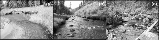
Channel types examined: (a) pool–riffle (Crane Creek), (b) plane bed (Camas Creek), and (c) step pool (Crawfish Creek) (from Faux et al. 2009).
Methods
Habitat measurements were made at each of the 12 sites using monitoring protocols developed, or used, by seven monitoring groups. We define monitoring groups as independent groups that assess a suite of stream habitat attributes. Protocols are defined as the monitoring group's specific methodologies (including operational definitions, procedures, and training) used to evaluate a suite of attributes. The seven monitoring groups evaluated in this study were the U.S. Forest Service and Bureau of Land Management (USFS–BLM; aquatic and riparian effectiveness monitoring program [AREMP]; AREMP 2005), the California Department of Fish and Game (CDFG; Downie 2004), the U.S. Environmental Protection Agency (environmental monitoring assessment program [EMAP]; EPA 2006b), the Northwest Indian Fisheries Commission (NIFC; Pleus and Schuett‐Hames 1998; Pleus et al. 1999; Schuett‐Hames et al. 1999), the Oregon Department of Fish and Wildlife (ODFW; Moore et al. 1997), the USFS–BLM (biological opinion effectiveness monitoring program [PIBO]; Dugaw and coworkers, unpublished manual on monitoring streams and riparian areas [available: http://www.fs.fed.us/]), and the upper Columbia monitoring strategy (UC; T. W. Hillman, unpublished report on a monitoring strategy for the upper Columbia basin). The references cited here for each group refer specifically to their 2005 field methods, which were used during this study.
Field crews from each monitoring group sampled a suite of stream habitat attributes at each site following their program's protocols (see exception below), each crew beginning at the same starting point and moving upstream a length defined by their protocol (reach lengths of 20–40 bank‐full widths). Average reach lengths evaluated by the monitoring groups ranged from 150 to 388 m (overall average = 256 m; SD = 104 m). Three groups—CDFG, NIFC, and ODFW—evaluated a shorter length of stream than their protocols normally require (approximately 40 times bank‐full width) to facilitate comparisons for this study. Modification of a group's standard protocol could lead to nonrepresentative results, but our goal was to compare results obtained over similar sampling domains (i.e., reaches that were 20–40 bank‐full widths in length).
Each monitoring group evaluated a stream reach using a minimum of two independent crews. All crews conducted surveys during summer low flow (July 15 to September 12, 2005) and were instructed to “tread lightly” to minimize impact to the channel parameters being measured over the course of the site visits by each of the monitoring groups and their crews. Visual inspection of channel characteristics before and after the study showed little impact of the crews on the measured parameters. Crews completed measurements at each stream in a single day, and all reaches were worked on by only one crew at a time except when precluded by logistics. Of the 236 total site visits conducted for this study, two crews were at the same site on the same day only 13 times (<6% of the time).
Crews were selected from each group based on availability and logistics, and not on experience; as such, results from each crew are considered typical for a given monitoring group. The sampling objective was to maximize the total number of crews each group used and randomize their sampling effort across the sampling time frame. Logistical constraints, however, led to differences in the number of unique crews each monitoring group used as well as the time period within which each group took to complete all sampling (i.e., the total number of days from the first to last day of sampling; AREMP = 6 crews/7 d to sample all sites, CDFG = 3 crews/15 d, EPA = 3 crews/27 d, NIFC = 3 crews/25 d, ODFW = 2 crews/37 d, PIBO = 6 crews/33 d, and UC = 3 crews/10 d).
We present data on a selection of 10 physical attributes that were measured by the majority of the monitoring groups. These attributes can be divided into four broad classes: (1) overall reach characteristics (channel gradient and sinuosity), (2) channel cross‐section characteristics (mean bank‐full width and width‐to‐depth ratio), (3) habitat composition (percent pools, pools/km, and mean residual pool depth [RPD]), and (4) bed material and channel roughness (median particle size [D50], percent fines, and large woody debris [LWD]/100 m). We provide definitions of the above attributes and a summary of how each monitoring group collected these data in Appendix 1. Many of the groups use methods borrowed from one another, with modifications in some instances, but the approaches are largely variants on the same theme.
In addition to the data collected by the monitoring groups, intensive (i.e., more‐detailed) measurements were conducted by staff from the U.S. Forest Service's Rocky Mountain Research Station (RMRS) in an effort to gain more accurate and precise estimates of attribute values compared with the rapid field techniques used by the monitoring groups in this study. Previous studies have compared internal consistency within groups (e.g., Marcus et al. 1995; Roper and Scarnecchia 1995; Olsen et al. 2005) and compatibility across groups (Wang et al. 1996; Larsen et al. 2007; Whitacre et al. 2007), but not accuracy of measurements. Accuracy and precision may be an issue with the monitoring groups examined in this study as they employ rapid measurement techniques designed to allow sampling of one or more sites per day, resulting in fewer measurements with generally less‐precise equipment than the intensive measurements conducted by RMRS (Appendix 1).
The RMRS crew measured attributes over reaches that were 40 bank‐full widths in length, channel and flood plain topography being surveyed with a total station (874–2,159 points surveyed per site; 0.4–3.7 points/m2; 21–57 points per square bank‐full width). Cross sections were spaced every half bank‐full width along the channel (81 cross sections per site), and the bed material was systematically sampled using a grid‐by‐number pebble count (Kellerhals and Bray 1971; 10 equally spaced grains per cross section, 810 particles per reach), grains being measured with a gravelometer (e.g., Bunte and Abt 2001). At each site, a longitudinal profile of the channel center line was surveyed with the total station, and the number, position, and function of LWD was inventoried (Robison and Beschta 1990; Montgomery et al. 1995), LWD defined as having a length of 1 m or more and a diameter of 0.1 m or more (Swanson et al. 1976). Pools were visually identified as bowl‐shaped depressions (having a topographic head, bottom and tail), residual depths being determined from total station measurements of pool bottom and riffle crest elevations. The average width and length of each pool were measured based on channel morphology and topographic breaks in slope rather than on wetted geometry. Pools of all size were measured, without truncating the size distribution for requisite pool dimensions, and were classified as either self‐formed or forced by external obstructions (Montgomery et al. 1995; Buffington et al. 2002). These RMRS surveys required three people, working 4–9 d at each site, depending upon stream size and complexity. A single crew was used for all sites, and no repeat sampling was conducted. Because of time constraints, RMRS data were only collected at 7 of the 12 study reaches (PB = two streams, PR = two streams, and SP = three streams).
Overall, the RMRS crew used more precise instruments than the monitoring groups (Appendix 1): the total station yields millimeter‐ to centimeter‐level precision for measuring stream gradient, channel geometry (width, depth), sinuosity, and RPDs; and the gravelometer reduces observer bias in identifying and measuring b‐axis diameters of particles (Hey and Thorne 1983). Furthermore, the much higher sampling density of measurements conducted by RMRS provided more precise estimates of parameter values (mean, variance). Finally, the RMRS crew was generally more experienced, composed of graduate students and professionals trained in fluvial geomorphology, while the monitoring groups typically employ seasonal crews with more diverse backgrounds and less geomorphic training. For these reasons, the RMRS measurements were assumed to be of higher precision and accuracy and therefore used as a standard for comparison in this study.
Attribute evaluations
To assess performance and the potential for data sharing among monitoring groups, we evaluated (1) consistency of measurements within a monitoring group, (2) ability to detect environmental heterogeneity among streams, (3) compatibility of measurements among monitoring groups, and (4) relation of measurements to values determined from the more intensive sampling. While statistical tests are used where appropriate in our analysis, most of our comparisons are evaluated in terms of threshold criteria. Furthermore, because many environmental variables have skewed distributions that often fit the lognormal distribution (Limpert et al. 2001) and are often log transformed prior to analysis, we evaluated how transformations might affect our conclusions based on these criteria. We present results of two attributes that are commonly log transformed (D50 and LWD/100 m) in both untransformed units (additive error) and in logarithmically transformed values (multiplicative error; Limpert et al. 2001). We used the natural log (loge) for all transformations and added 0.1 to all LWD values prior to transformation to remove zero values at sites where no LWD was observed.
Consistency of measurements within a monitoring group
We assessed a monitoring group's consistency by calculating the root mean square error (RMSE = the square root of the among‐crew variance [i.e., SD]) and the coefficient of variation (CV = [RMSE/mean] × 100) for each attribute measured by each monitoring group. The RMSE of a given channel characteristic represents the average deviation of crew measurements within a given monitoring group across all sites, and the CV is a dimensionless measure of variability scaled relative to the grand mean across all sites (Zar 1984; Ramsey et al. 1992; Kaufmann et al. 1999). Using these measures, if all crews within a monitoring group produce identical results at each site, both RMSE and CV would be 0. We used analysis of variance (ANOVA [each of the 12 streams as a block]) to estimate the grand mean (mean value of the 12 streams averaged over the crew observations for each stream), RMSE, and CV for each of the attributes evaluated by each of the monitoring groups.
The exact value of RMSE defining high, moderate, and low consistency is expected to differ by attribute and by differences in protocols among monitoring groups. Use of RMSE as a measure of consistency is best done when the investigator understands the attribute of interest and how much change in the attribute is meaningful (Kaufmann et al. 1999). Since the use of RMSE as a criterion is dependent upon the situation, we specify the values we consider to represent high, moderate, and low consistency for each parameter examined in this study (Table 2). These RMSE criteria represent what we consider to be meaningful differences in the measured attributes; however, care should be used when applying these criteria to other situations.
Root mean square error values used as indicators of consistency (repeatability) among observers. The values chosen for high consistency were indicative of observer differences that would have small biological or physical consequences, while those chosen for low consistency would have substantial consequences. Abbreviations are defined in Table 1
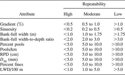
Root mean square error values used as indicators of consistency (repeatability) among observers. The values chosen for high consistency were indicative of observer differences that would have small biological or physical consequences, while those chosen for low consistency would have substantial consequences. Abbreviations are defined in Table 1
In contrast to RMSE, CV is a normalized parameter that can be compared across attributes and groups. We defined a protocol as having high consistency when the CV was less than 20%. This value was chosen because when the CV is low it greatly reduces the number of samples necessary to detect changes (Zar 1984; Ramsey et al. 1992). We defined CV values between 20% and 35% as having moderate consistency. While the upper value (35%) is somewhat subjective, it was chosen because values within this range should facilitate classification (e.g., deciding which class a stream is in) but would be less reliable for comparing mean values across time or space without numerous samples. Finally, CVs greater than 35% were defined as having low consistency because the average difference among observers within a group is greater than one‐third the mean. This would suggest that meaningful classification might be difficult (e.g., different observers within the same monitoring group could classify the same stream differently; Roper et al. 2008), making statistical comparisons in time or across locations extremely expensive or impossible due to sample size requirements. A caveat regarding the use of CV is that results can be misleading if regional values are applied to specific field applications because the local and regional means may differ (Kaufmann et al. 1999). Overall, values of RMSE and CV in this study resulted in similar estimates of consistency. When these two metrics differed, we used the value that suggested the greater consistency. We used the value that suggested the higher consistency for comparisons in this paper but suggest researchers decide this on a case‐by‐case basis depending on how important detection of change in a specific metric is to their particular study.
Adequacy of a monitoring group's protocol to detect environmental heterogeneity
The ability of a protocol to detect environmental heterogeneity was evaluated using a signal‐to‐noise (S:N) ratio, which quantifies the difference among streams (signal) relative to the difference among individuals evaluating a stream (noise; Kaufmann et al. 1999). To determine the S:N ratio, a random‐effects ANOVA model was used to decompose the total variance into that associated with differences among streams versus variation in crew observations at a stream (all error not due to the main effect of stream site is treated as observer variability; Roper et al. 2002). An S:N ratio of 1 indicates that the variation in an attribute among a set of streams is equal to the variation among observers in evaluating those streams. For reasons described in the next section, we characterize the likelihood of detecting environmental heterogeneity as high when S:N ratio is greater than 6.5, moderate when S:N ratio is between 2.5 and 6.5, and low when S:N ratio is less than 2.5.
Relationships among protocols for a given attribute: Data crosswalks and sharing
For monitoring groups to share data, the values for a measured attribute must be related to each other (i.e., correlated). Correlation requires that S:N ratios, as reflected in the following equation, be high (Faustini and Kaufmann 2007):

where  is the theoretical maximum coefficient of determination (r2) between two protocols, and the numeric subscripts indicate the respective protocols. Based on the above equation, if protocols for the same attribute measured by two different monitoring groups had S:N ratios greater than 6.5, then
  could be 0.75 or higher. As such, if S:N ratios are high, it becomes possible to determine whether one protocol is highly correlated to another. In contrast, S:N ratios of ∼2.5 would result in an
  of only 0.5 (moderate correlation). When S:N ratios are less than 2.5, they are considered low because even if monitoring groups are measuring the same attribute, variation among observers within a group precludes detecting a relationship (low correlation). While the exact S:N thresholds are somewhat subjective, they meet our objective of providing criteria that assess the likelihood for monitoring groups to share data.
In addition to correlation, results obtained by each monitoring group should be accurate; correlation among groups does not guarantee accuracy of their measurements. Since it is difficult to know the true value of a given attribute, we evaluated compatibility of data among the monitoring groups using two approaches: (1) assessing whether attribute values were correlated between monitoring groups and across channel types (both in terms of the above S:N criteria and  ‐values), and (2) by comparing the results of each monitoring group to the RMRS data (intensive measurements that are used as a standard for accuracy in this study, as discussed above). (For the second approach, we considered correlations to be high when r2 > 0.75, moderate when 0.5 < r2 < 0.75, and low when r2 < 0.5.) We also calculated Cook's distance for each regression to determine if any stream had a significant effect on the relationship. As a rule of thumb, an observation has a heavy influence on a relationship when Cook's distance exceeds 1 (Dunn and Clark 1987).
To further compare results of the monitoring groups with each other, we evaluated whether mean estimates of a given attribute in a given channel type (PB, PR, and SP) were related. We used channel types for this comparison to minimize the influence of individual crew observations at a single stream (i.e., by using group means within streams). Replicates within channel types permitted estimation of both main effects (channel type and monitoring group) and interactions (see below).
Furthermore, channel attributes are expected to differ among channel types (e.g., Rosgen 1996; Buffington et al. 2003), and these differences should be detectable by each of the groups as part of their status‐and‐trend monitoring. Moreover, there is the potential for protocols to be biased by channel type; because of how a given protocol is defined or implemented, it may systematically over‐ or underestimate a given attribute. To examine these issues, we tested for a significant interaction (P < 0.1) using ANOVA, channel type and monitoring groups as the main effects and observers within a stream as a repeated measure (i.e., average of all crews for each stream). A significant interaction effect can be present if one group has a consistent measurement bias that varies with channel type. For example, if group A consistently measures bank‐full width wider than group B in PB channel types but group A measures bank‐full width narrower than group B in PR channel types, then this will result in an interaction effect. Alternatively, even if the same trend across channel types is observed for an attribute among all protocols (e.g., PB > PR > SP), a significant interaction can exist if the difference in mean among protocols changes among channel types. Examples of these types of interactions are presented in graphical form in Results.
Ideally, data could be shared among groups even if both main effects (channel type and monitoring group) were significantly different as long as there was no significant interaction. This result would suggest that the underlying attribute that the monitoring groups are measuring is different but correlated. When significant interactions were found, we graphed the resulting data to determine which monitoring groups exhibited patterns that differed from the others. If these graphs suggested such a result, we reran the analysis after excluding data from monitoring protocols that differed from the others to determine if the interaction was still significant.
Results
Consistency of Measurement within a Monitoring Group
Gradient and sinuosity were generally measured with high internal consistency (Table 3). Four of the six monitoring groups that measured gradient had RMSE values less than 0.5%, while the other two groups had values between 0.5% and approximately 1.0%. The four groups that measured gradient with RMSE less than 0.5% also had CV less than 20% (high consistency); the other two groups had CV less than 35% (moderate consistency for gradient). All four monitoring groups that measured sinuosity had RMSE less than 0.1 and CV less than 20%.
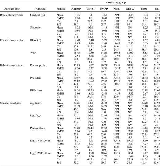
Descriptive statistics for attribute data collected by individual monitoring groups for all channel types combined. Statistical abbreviations are as follows: RMSE = root mean square error; CV = coefficient of variation; and S:N = signal–noise ratio; NM = not measured. See Table 1 for other abbreviations and text for monitoring group acronyms
Descriptive statistics for attribute data collected by individual monitoring groups for all channel types combined. Statistical abbreviations are as follows: RMSE = root mean square error; CV = coefficient of variation; and S:N = signal–noise ratio; NM = not measured. See Table 1 for other abbreviations and text for monitoring group acronyms
Consistency in measuring mean bank‐full width and width‐to‐depth ratio was lower (Table 3). Three of the seven monitoring groups had values of RMSE less than 1 m and CV less than 20% for bank‐full width. Two monitoring groups had CV values less than 20% for measurements of width‐to‐depth ratio, but none had RMSE less than 2. Consistency in measuring habitat composition was mixed; RPD was generally measured with high internal consistency (RMSE ≤ 5 cm and CV < 20% for six out of seven monitoring groups), while measurements of percent pools and pools per kilometer were less consistent (none of the monitoring groups had a CV < 20% or RMSE < 5 for either of these attributes). The percent fines was generally measured with moderate to low consistency, while D50 was generally measured with low consistency and estimates of LWD/100 m varied from high to low consistency (Table 3).
Although consistency of sediment metrics was generally low (D50) to moderate (% fines), these metrics were likely sufficient to distinguish broad differences in D50 (i.e., differentiating sand‐, gravel‐, and cobble‐bedded channels) and to distinguish critical thresholds for fine sediment (e.g., the 20% threshold for declining survival to emergence of salmonid embryos; Bjornn and Reiser 1991). The use of logarithmic transformations for D50 did not change results in terms of CV categories (low, moderate, high consistency). In contrast, logarithmic transformation of LWD/100 m had a negative effect on consistency estimates; two monitoring groups (ODFW and PIBO) went from moderate or high internal consistency (CV < 35%) to low internal consistency (CV > 35%).
Adequacy of a Monitoring Group's Protocol to Detect Environmental Heterogeneity
Three attributes (channel gradient, mean bank‐full width, and loge [LWD/100 m]) had moderate (>2.5) or high S:N ratios (>6.5) across all monitoring groups (Table 3). Two other attributes (RPD and loge [D50]) had S:N ratios greater than 2.5 for the majority of the monitoring groups that measured them (Table 3). The remaining five (variables, sinuosity, width‐to‐depth ratio, percent pools, pools per kilometer, and percent fines) had low S:N ratios (<2.5) for at least 50% of the monitoring groups. Two of the seven monitoring groups (ODFW and NIFC) had S:N ratios greater than 2.5 for more than 80% of the channel attributes evaluated when transformed values of D50 and LWD/100 m were considered (Table 3). Two groups (AREMP and EMAP) had S:N ratios greater than 2.5 for 70% of the attributes. One monitoring group (PIBO) had S:N ratios greater than 2.5 for 60% of the measured attributes. Two groups (UC and CDFG) had S:N ratios greater than 2.5 for 50% or less of their measured attributes.
Relationships among Protocols for a Given Attribute: Data Crosswalks and Sharing
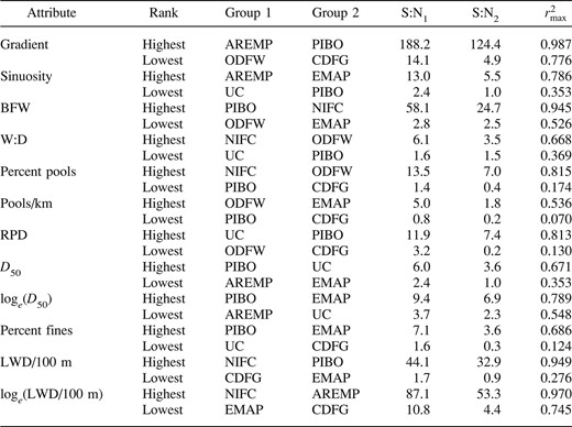
The potential to share data were highly dependent upon the attribute and the monitoring group. For example, measurements of channel gradient had very high S:N ratios (>10) for five of the six monitoring groups, suggesting that data for this attribute have a high potential of being shared (Tables 3, 4). In contrast, six of the seven groups that determined pools per km had an S:N ratio less than 2.5 (low likelihood of sharing), the remaining group having an S:N ratio of 5. The generally high S:N ratio (all but one group > 2.5) for measurements of gradient, bank‐full width, RPD, loge (D50) and loge (LWD/100 m) suggest that these attributes have the greatest potential for being shared among groups (Tables 3, 4). In contrast, values of width to depth, percent pools, and pools per kilometer may be difficult to share because of generally low S:N ratios (<2.5).
Theoretical maximum correlation coefficients (  ; Faustini and Kaufmann 2007) for attribute values measured by different pairs of monitoring groups for all channel types combined. The
  = values are presented for the highest and lowest S:N results for each attribute. See text for a list of monitoring group and attribute acronyms
Theoretical maximum correlation coefficients ( ; Faustini and Kaufmann 2007) for attribute values measured by different pairs of monitoring groups for all channel types combined. The = values are presented for the highest and lowest S:N results for each attribute. See text for a list of monitoring group and attribute acronyms
Protocols used by monitoring groups to measure channel gradient, sinuosity, pools per kilometer, and D50 had similar trends across channel types (no significant interactions; P > 0.1; see gradient and D50 for examples in Figure 3). Statistically significant interactions (indicating systematic differences among protocols) were found for bank‐full width, width‐to‐depth ratio, percent pools, RPD, percent fines, and LWD. Because the characteristics of LWD and percent fines are defined differently by different monitoring groups (Appendix 1), it is not surprising to see a significant interaction for these attributes. Consequently, those data may be more difficult to share because the monitoring groups are not measuring the same underlying condition (i.e., different LWD size categories and different definitions of how and where fine sediment is measured; Appendix 1).
![Comparison of monitoring groups' results for six attributes averaged by channel type (plane bed [PB], pool–riffle [PR], and step pool [SP]). There are no interactions between the measurements for two attributes—channel gradient and median grain size (D50)—but significant interactions between those for the other attributes. See Methods for descriptions of the types of interactions and group acronyms.](https://oup.silverchair-cdn.com/oup/backfile/Content_public/Journal/najfm/30/2/10.1577_M09-061.1/5/m_nafm0565-fig-0003-m.jpeg?Expires=1750758751&Signature=v3HgvubPmANwJPC1VVdSNn5oUZXZowMbKgmCCiqT5H1Jsku8sHJAdZKvIFXO3BBKH71BqVIazz4lXBS296Frn79Eq5xxormDp5sOit9LHjgMiw-rhA-THE64zf3ZXxh6Ze9xqsjVwhc-Yc7xqZDEKuB9CKjaJLsMa2kucDDY08S~hPC~O7Y14Z9dhh-n6TpSnYxBydQ5ZGchdhlVh2tYKkZtzMwS04jcZxKOSa7CWpN3XOrL7aNSvyKmer6etiZHu1UWoy89WZkUTpPLIjCcJ5uZeqnJO5AmpwmMnJfwG84jFdWi-ycCwLykU9pxuTWquU9RtJ8P7YA6UiigLh8vxw__&Key-Pair-Id=APKAIE5G5CRDK6RD3PGA)
Comparison of monitoring groups' results for six attributes averaged by channel type (plane bed [PB], pool–riffle [PR], and step pool [SP]). There are no interactions between the measurements for two attributes—channel gradient and median grain size (D50)—but significant interactions between those for the other attributes. See Methods for descriptions of the types of interactions and group acronyms.
We found that significant interactions in several of the attributes (bank‐full width, width‐to‐depth ratio, and percent pools) became nonsignificant when results from one or two monitoring groups were removed. Percent pools no longer had a significant interaction when CDFG and EMAP data were removed; this was because these two groups observed smaller percentages of pools in pool–riffle streams than in step‐pool and plane‐bed channels, while the remaining groups found that pool–riffle sites had a greater percentage of pools than step‐pool and plane‐bed streams (Figure 3). The width‐to‐depth ratio interaction was no longer significant when AREMP and CDFG data were removed; this was because these groups observed larger width‐to‐depth ratios in step‐pool streams than in pool–riffle channels, while the remaining groups observed the reverse. The interaction in RPD was due to the EMAP and NIFC groups finding greater pool depths in plane‐bed channels than in pool–riffle streams, while the remaining groups found the opposite. Results for bank‐full width differed from those above because the significant interaction arose from the magnitude of the differences among channel types rather than differences in their trends (Figure 3). Although there was no significant interaction for pools per kilometer, the high within‐group variation in measuring this attribute results in low statistical power to detect differences among groups and poor potential for sharing this attribute (Tables 3, 4).
Comparison of measured attributes with results obtained by the RMRS team was similarly uneven (Table 5). We found that the monitoring groups' measurements of channel gradient, sinuosity, and D50 (both transformed and untransformed) were highly correlated with the RMRS measurements of those attributes (r2 > 0.75). Measurements of bank‐full width were moderately correlated with the RMRS values (0.50 < r2 <0.75), but this correlation would have been higher (r2 > 0.80) if not for consistent differences between the monitoring groups and the RMRS measurements at two sites (Figure 4; Bridge and Crane creeks). Correlations between width‐to‐depth values measured by the monitoring groups and the RMRS team were uniformly low (r2 < 0.50). There was a generally high correlation between monitoring group and RMRS measurements of percent pools for six of the seven monitoring groups. However, the relationship was dominated by Crane Creek, which had the largest abundance of pools (Cook's distance = 1–55 across the monitoring groups). Consequently, additional data collection over a broader range of conditions is warranted to further test the observed relationships. In contrast, the between‐group correlation of pools per kilometer is uniformly poor.
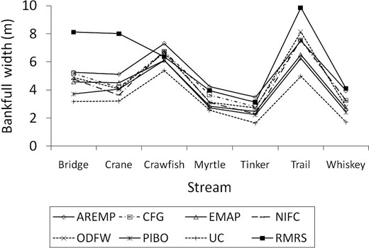
Comparison of mean bank‐full width as determined by the seven monitoring groups and via the more intensive data collection (RMRS) at 7 of the 12 study sites.
Coefficients of determination (r2) between the values of the more intensively measured attributes and those obtained by individual monitoring groups for all channel types combined. See text for monitoring group and attribute acronyms
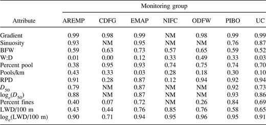
Coefficients of determination (r2) between the values of the more intensively measured attributes and those obtained by individual monitoring groups for all channel types combined. See text for monitoring group and attribute acronyms
We found that the strength of between‐group relationships for measured wood loading (LWD/100 m) was partially dependent on whether the data were transformed or not. Five of seven groups had r2 greater than 0.5 for untransformed values, but transformation resulted in all groups achieving r2 greater than 0.5. Inspection of these relationships reveals that they are dominated by data from a single site. The relationships for untransformed LWD/100 m are driven by agreement across all groups that Bridge Creek has no LWD. When transformed, Bridge Creek became an outlier (Cook's distance > 8 for all monitoring groups) because its wood count was many units less than the other sites (e.g., loge [0 + 0.1] = −2.3 for 0 pieces of wood versus loge [1 + 0.1] = 0.095 for 1 piece/100 m). In contrast, the regression for the untransformed data had no heavily weighted observation (Cook's distance < 1 for all but one monitoring group). Overall, there was a moderate correlation (r2 > 0.50) between monitoring groups and RMRS values for at least 50% of the channel attributes except for the CDFG group (Table 5).
Summary
In almost every case, there were one or more groups that either measured an attribute with less consistency or seemed to be measuring a slightly different underlying environmental condition than the other groups (Table 5). However, the study results indicate that measurements were relatively consistent within each monitoring group (moderate to high consistency) and that there is a moderate to high likelihood for sharing data if monitoring groups alter their protocols for attributes that had significant interactions. Overall, four of the seven monitoring groups measured at least 80% of the evaluated attributes with moderate or high consistency (CV < 35%, high‐to‐moderate RMSE, or both; AREMP, 80% of the evaluated attributes; NIFC, 83.3%; ODFW, 88%; and PIBO, 80% [note that these summaries include the best of the raw or log‐transformed values]). Two of the remaining monitoring groups (EMAP, UC) measured the majority of the attributes with moderate or high consistency, while CDFG measured 50% of the attributes with moderate or high consistency (Table 6).
Overall assessment of the performance of monitoring groups, scored as high (H), moderate (M), or low (L); NM = not measured. Three performance characteristics are scored for each monitoring group: Internal consistency (CV, RMSE, or both), environmental heterogeneity (S:N), and likelihood for sharing data (correlations with intensive data); H, M, and L values are defined in the text for each of these parameters. See text for a list of monitoring protocol and attribute acronyms

Overall assessment of the performance of monitoring groups, scored as high (H), moderate (M), or low (L); NM = not measured. Three performance characteristics are scored for each monitoring group: Internal consistency (CV, RMSE, or both), environmental heterogeneity (S:N), and likelihood for sharing data (correlations with intensive data); H, M, and L values are defined in the text for each of these parameters. See text for a list of monitoring protocol and attribute acronyms
Two attributes, channel gradient and sinuosity, were consistently measured within monitoring groups (low‐to‐moderate CV and RMSE) and produced values that were correlated both among monitoring groups and with the RMRS data (high r2; Tables 4, 5). Gradient also had generally high environmental heterogeneity (S:N > 6.5), but sinuosity varied over a relatively narrow range, leading to low S:N values (<2.5) for two of the four protocols that measured it. Data on a third attribute (RPD) also was measured with high consistency, had high S:N ratios, and could likely be shared among a majority of the groups. Evaluations of LWD/100 m had moderate‐to‐high internal consistency but would be difficult to share because of differences in sampling protocols (Appendix 1) and resultant differences in measured values (Figure 3).
Bank‐full width, D50 (both transformed and untransformed), percent pools, and percent fines were generally measured with less consistency within each group and typically had smaller S:N ratios than the previously listed attributes, but had values that were moderately or highly correlated with each other and to the RMRS data. Width‐to‐depth ratios and pools per kilometer were generally inconsistently measured, had low environmental heterogeneity, and were weakly correlated to the RMRS data.
Overall, we found that five monitoring groups (AREMP, EMAP, ODFW, PIBO, and UC) measured two‐thirds or more of the attributes with high internal consistency, had moderate S:N ratios, and produced results that were at least moderately related to those of the other groups and the RMRS data. One group (NIFC) measured attributes with high internal consistency but had fewer attributes related to the results of the other groups or to the RMRS data and collected fewer of the commonly evaluated stream attributes. California Department of Fish and Game measured attributes with lower average internal consistency and were not as strongly correlated to the results of the other monitoring groups.
Discussion
Our comparison of seven stream habitat monitoring groups from the Pacific Northwest suggests considerable variability in each group's ability to consistently and accurately measure some stream attributes. Reasons for differences in observer measurements have been studied elsewhere and include differences in the duration of training (Hannaford et al. 1997; Whitacre et al. 2007; Heitke et al. 2008), level of experience (Wohl et al. 1996; Heitke et al. 2008), operational definitions for the attribute of interest (Kaufmann et al. 1999; Heitke et al. 2008; Roper et al. 2008), intensity of measurements (Wolman 1954; Wang et al. 1996; Robison 1997), when and where the attribute is measured (Olsen et al. 2005; Roper et al. 2008), and characteristics of the sampled stream reach (Whitacre et al. 2007).
Regardless of the exact reason for poor performance of a monitoring group (e.g., low repeatability, poor accuracy, etc.), we argue improvement can only occur if groups and protocols are regularly evaluated and training and oversight are thorough and ongoing. Assessment of groups and protocols may identify weaknesses that can then be remedied. For example, in an earlier study by Whitacre et al. (2007), it was found that PIBO had a higher internal consistency in measuring stream gradient than AREMP. This difference occurred even though AREMP used an instrument with greater precision (total station versus hand level). Whitacre et al. (2007) speculated that the presence of dense riparian vegetation caused the total station to be moved multiple times, resulting in greater cumulative survey errors by AREMP. Following this study, AREMP altered its protocols for measuring stream gradient and increased training. Results of the current comparison indicate that both PIBO and AREMP now measure gradient with high consistency. Comparison of results among monitoring groups, such as the one above, not only provides feedback on what is possible but can also provide incentive for improving a monitoring group's protocols.
Two concerns identified prior to implementing our study were how declining stream flows during the summer sampling period and different numbers of crews would affect study results. We found no strong evidence supporting either of these concerns. Changes in flow have the potential to cause variability within and between monitoring groups whose protocols rely on wetted channel dimensions. With the exception of RMRS, all of the groups examined in this study use wetted dimensions to some degree in their measurements (Appendix 1). Stream gradient, percent pools, and pools per kilometer depend on wetted dimensions for all groups, as does percent fines (except in the UC protocol). Three additional parameters (reach length, sinuosity, and D50) depend on wetted dimensions for the EMAP protocol. To document changes in flow during the study period, staff gauges were installed at each site. The maximum change in reach‐average width and depth was 17% and 33%, respectively, on average across the sites during the study period (excluding Tinker Creek, which went dry). The corresponding changes in stream gradient were small (0.8% on average across sites), but the effects of changing flow on the above‐listed parameters are not easily quantified. Examination of the within‐ and between‐group variability over the study period may offer some insight into the potential effects of declining flows. Both PIBO and NIFC maintained high consistency within their groups even though observers sampled over an entire month during which stream flows declined. In contrast, CDFG crews had lower repeatability even though they sampled over a 2‐week period. One reason why AREMP may have been able to determine pool attributes more consistently than PIBO was because base flows were more stable over the shorter time frame they sampled (7 versus 33 d). However, this would not explain why ODFW was able to consistently determine pool attributes despite sampling over a 37‐d time frame. Overall, these observations suggest that declining flows did not have a strong influence on internal consistency, but further examination of this issue is warranted. Sampling over a shorter period reduces within‐group variability due to changing flows but does not account for between‐group differences that may result from groups sampling different flows at different times of the study period.
The number of crews used (two to six) also seemed to have little relationship with consistency. The monitoring groups that sent more crews (AREMP and PIBO) may have been slightly more consistent, but ODFW only had two crews and were also consistent (Table 3). A possible reason for greater consistency with a larger number of crews is that anomalous results may be damped. For example, if a single crew provides a slightly different evaluation of a stream attribute, their results will have less impact if it is one of six crews rather than one of three crews. Certainly, the changes in base flow and the number of observers had some impact on the comparisons made in this study, but they do not appear to be significant.
Our results also anecdotally suggest that additional training may be required when crews are unfamiliar with the channel types they are sampling. All monitoring programs other than the CDFG had previous experience sampling streams similar to those present in the John Day River basin. The lack of experience in monitoring these systems may partially explain the lack of consistency within this program.
Comparing monitoring group results with more intensive site measurements (e.g., RMRS data) provided additional insight into the types of common errors associated with rapid monitoring protocols, such as those evaluated in this study. For example, in all but two streams there was a high correlation between bank‐full width measurements made by the monitoring groups and those determined from the RMRS data (Figure 4; Bridge and Crane creeks). This difference can be explained by examining cross‐section transects common to all of the field crews (five transects were established in each stream reach where all monitoring groups, including the RMRS team, measured the exact same cross section).
Bank‐full width is clearly visible in the cross section surveyed by the RMRS team at Bridge Creek (Figure 5), but monitoring groups consistently underestimated bank‐full width at this location. Based on photographs taken at the site and subsequent field visits at different times of year, it became apparent that the observed differences in bank‐full width measurements were due to dense seasonal riparian vegetation that obscured the bank morphology during the summer sampling period, causing field crews to underestimate channel dimensions. Comparisons of this sort highlight the value of periodically evaluating protocols and having quality assurance–quality control (QA–QC) plans. This was accomplished in this study by obtaining intensive measurements, establishing common sampling locations for calibrating and comparing the results of monitoring groups, interpreting discrepancies, and identifying areas for additional training (e.g., identifying bank‐full in brushy streams). Overall, the correlations between many of the attributes measured by the monitoring groups and the RMRS data were high (Table 5). This finding is encouraging considering that the monitoring group evaluations were conducted over different stream lengths (same starting point, but different ending locations), reach length potentially having a significant impact when comparing results among and within monitoring groups (Whitacre et al. 2007).
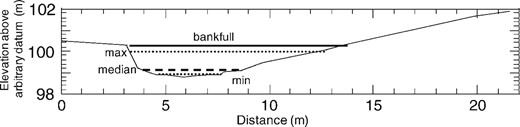
One of five cross sections at Bridge Creek that was measured by all monitoring groups and surveyed by the RMRS team. The line labeled “bank‐full” was determined from the RMRS data and field indicators. The maximum, minimum, and median bank‐full values were determined from the values reported by the monitoring groups. Most of the groups tended to underestimate the bank‐full width at this cross section (the median value is closer to the minimum) because vegetation obscured the bank‐full morphology.
We found that transforming data could affect estimates of internal consistency, S:N ratios, and relationships with more intensive measurements. Comparisons between transformed and untransformed data for both D50 and LWD/100 m suggest that the effects of transformation on CV and S:N ratios were mixed (Table 3), the exact effect dependent on the distribution of data across streams and among observers. However, transformations consistently had a positive effect on the correlation between measurements made by monitoring groups and the RMRS data collection. For D50, this improvement was due, in part, to the fact that the underlying data distribution was lognormal, even though the observer error distribution was not. In contrast, the improved correlation with transformation of the LWD/100 m was due to the influence of a single site (Bridge Creek) and its lack of LWD.
The use of logarithmic transformation often has biological or physical basis and has the advantages of offering a convenient approach for interpreting multiplicative effects and for producing confidence intervals that are always positive (Limpert et al. 2001). Use of this transformation can therefore aid our understanding of the system. This is not true of all transformations (such as ranks used for nonparametric tests or arcsine square root transformations), which may address statistical concerns but do not improve data interpretation (Johnson 1995). The possibility that different monitoring groups might have different error structures (e.g., if one group bins pebble size with the phi scale [Krumbein 1936] while another measures to the nearest millimeter) complicates the ability to join data because one must account for differences in both means and the error structure.
From a Blue Mountains ecoregion perspective, the relationship among monitoring groups and the RMRS data suggests the possibility of being able to combine (share) data from attributes with high internal consistency (CV < 20%, relatively low RMSE values, or both), high S:N ratios (>6.5), and high correlation (r2 > 0.75) with the intensive measurements (RMRS). In order to combine these data, it first would be necessary to clearly define the target population of interest (e.g., fish‐bearing streams) and provide consistent representation of the distribution of that target population across the landscape (e.g., a digital map of the stream network and potential habitat; Buffington et al. 2004) so that weights could be determined for each reach sampled by a monitoring group (Larsen et al. 2007).
The simplest way to analyze the combined data would be to treat monitoring groups as a block effect in a larger ANOVA design. Because of the difference in overall means among monitoring groups, this approach may not be helpful in assessing status, but it would help to evaluate trend since correlated protocols should show the same change over time. The second approach would be to combine data using the rank order of the reach (percentile) within a sample of stream reaches. This approach would be bolstered if specific stream reaches were measured by all monitoring groups so as to serve as comparison–correlation sites. Such an approach might permit the construction of cumulative frequency histograms using conditional probability analysis (Paul and McDonald 2005).
Both of these approaches will be hampered where interactions occur among values measured by different monitoring groups. A significant interaction will influence how a stream attribute is perceived to change through time. This can affect the rank order of stream attributes among monitoring groups (i.e., how consistently a monitoring group measures an attribute compared with other groups) and will prevent data crosswalks. Therefore, combining data among monitoring groups, though conceptually straightforward, should be done with care and, in some cases, may not be feasible.
Conclusions and Recommendations
For each of the 10 attributes we evaluated, at least one monitoring group was able to simultaneously achieve at least moderate internal consistency (CV< 35% and low‐to‐moderate RMSE) and moderate detection of environmental heterogeneity (S:N > 2.5). However, none of the monitoring groups were able to achieve this standard for all their measured parameters, suggesting that there is room for improvement in all the monitoring groups evaluated in this study, both for internal program success and the possibility of sharing data and scaling up results to regional and national levels.
This study was conducted on a limited number of streams, over a limited area, and over a protracted sampling period that could have influenced the results due to changes in streamflow. We also recognize that the criteria used here for evaluating protocol performance and compatibility will not necessarily fit every situation or management objective. However, some sort of criteria are needed for evaluating data collected by monitoring groups; poorly measured attributes add little to our understanding of streams and provide fodder for articles questioning the need for, or validity of, large‐scale monitoring groups (GAO 2000, 2004; Stem et al. 2005; Nichols and Williams 2007). To ensure that data are efficiently collected, we suggest that agencies and organizations either adopt standards such as those used in this analysis or develop other meaningful criteria for aquatic habitat data, and implement an annual QA–QC program. There is always a trade‐off between rigor at a site and the benefits gained from visiting more sites. However, greater measurement precision and consistency increase the likelihood that data can be combined across groups, in turn increasing the number of monitoring sites available for combined analysis.
We recognize that the loss of legacy data are a primary concern for monitoring groups when considering new or modified protocols (Bonar and Hubert 2002). The power of using protocols that capture legacy data are well demonstrated by McIntosh et al. (1994; historic changes in pool size and frequency in the Columbia basin) and Rodgers et al. (2005; use of basin surveys to augment random surveys in an assessment of carrying capacity for juvenile coho salmon Oncorhynchus kisutch in Oregon coastal drainages). However, if legacy data cannot be integrated into regional assessments or do not allow trend detection because of low measurement repeatability, there is little justification for spending limited resources to continue acquiring these data.
Our results, in combination with an earlier study (Whitacre et al. 2007), suggest that major improvement in monitoring group precision and consistency can occur without changing protocols. To do this it is first necessary to identify inconsistent protocols. Once a procedure within a protocol has been identified as being inconsistent (e.g., by evaluating how different observers make observations at a variety of selected locations; Figure 5), the protocol can be altered by either clarifying the operational definition or by providing additional training focused on aspects of the protocol that have been applied inconsistently.
The compelling reason to improve current protocols is the growing need to determine status and trends of stream habitat at a regional and national scale while being fiscally responsible (GAO 2000, 2004; EPA 2006a). There has been progress on (1) sampling designs that foster regional and national estimates of aquatic conditions (Urquhart et al. 1998; Larsen et al. 2001), (2) methods for combining data based on different sampling designs (Larsen et al. 2007), and (3) understanding which stream habitat attributes should be measured (MacDonald et al. 1991; Bauer and Ralph 2001; Montgomery and MacDonald 2002), but there has been little progress toward ensuring that monitoring groups incorporate QA–QC as part of their monitoring procedures. From an accountability standpoint, we think it is incumbent on managers of stream monitoring groups to be able to demonstrate that long‐term stream habitat monitoring efforts provide a cost‐effective assessment of habitat trends (Lovett et al. 2007). This goal will be best achieved by continually having monitoring groups assess data quality and by increasing coordination among monitoring organizations to improve data quality, reduce redundancy, and promote data sharing.
Acknowledgments
We thank the Independent Scientific Advisory Board (Northwest Power and Conservation Council) for study plan comments, and we thank two anonymous reviewers and the associate editor for constructive comments that improved the manuscript. The University of Idaho provided field equipment that was ably used by Patrick Kormos, Darek Elverud, Russ Nelson, Brian Ragan, and Kathy Seyedbagheri. This project was a collaborative effort of the Pacific Northwest Aquatic Monitoring Partnership and was funded by US Forest Service, Environmental Protection Agency, Bureau of Land Management, NOAA Fisheries, U.S. Fish and Wildlife Service, Bonneville Power Administration, the states of Washington, Oregon, and California, and the Northwest Indian Fisheries Commission.
Appendix 1
Monitoring Group Protocols
Summary of monitoring group protocols for measuring stream attributes examined in this study. Some protocols modified as noted in the descriptions presented here
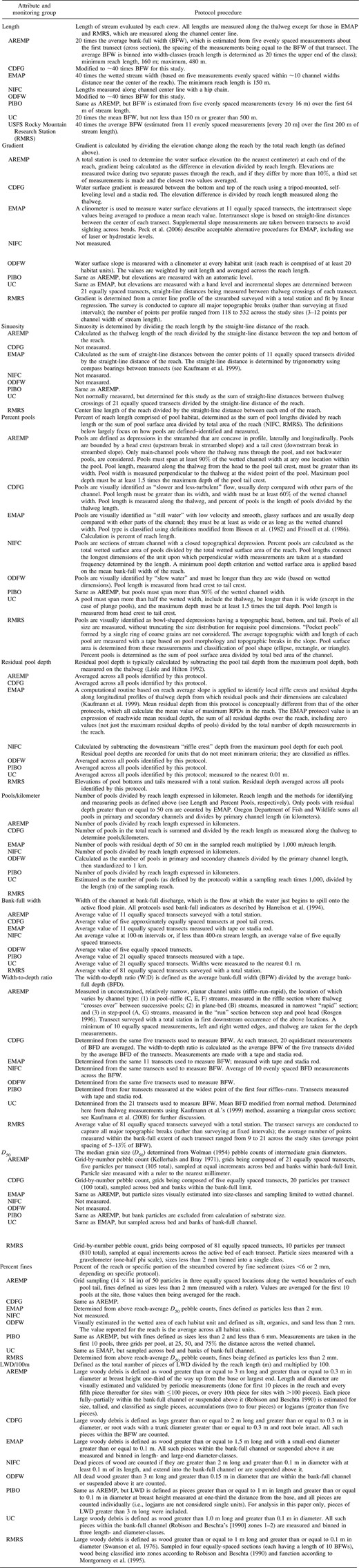
Summary of monitoring group protocols for measuring stream attributes examined in this study. Some protocols modified as noted in the descriptions presented here
