


ABSTRACT
In this paper, we propose a new approach to determining cosmological distances to active Galactic nuclei (AGNs) via light travel-time arguments, which can be extended from nearby sources to very high redshift sources. The key assumption is that the variability seen in AGNs is constrained by the speed of light and therefore provides an estimate of the linear size of an emitting region. This can then be compared with the angular size measured with very long baseline interferometryer to derive a distance. We demonstrate this approach on a specific well-studied low-redshift (z = 0.0178) source 3C 84 (NGC 1275), which is the bright radio core of the Perseus Cluster. We derive an angular diameter distance including statistical errors of |$D_{\mathrm{ A}} = 72^{+5}_{-6}$| Mpc for this source, which is consistent with other distance measurements at this redshift. Possible sources of systematic errors and ways to correct for them are discussed.
1 INTRODUCTION
2 METHODS
3 OBSERVATIONS
We obtained publicly available1 high-resolution maps of the source at 7 mm (43 GHz) observing wavelength from the Boston University blazar monitoring (VLBA-BU-BLAZAR) program (Jorstad et al. 2005, 2017). In practice, VLBI observations are measuring the incomplete Fourier transform of the sky brightness distribution, from which an image is produced using the clean algorithm (Högbom 1974) and phase and amplitude self-calibration. In order to parametrize features within these images, we fitted elliptical or circular Gaussian models directly to the interferometric visibilities, providing us with angular size and flux density measurements of emission regions within the map. We performed this analysis using standard routines in the program difmap (Shepherd 1997). To ensure amplitude calibration accuracy, the total VLBI flux densities were compared against total intensity measurements of the source and corrected accordingly if needed (e.g. Kim et al. 2019). The maps are shown in Fig. 1. We use these model-fitted flux densities as the measurements from which the light curve shown in Fig. 2 is derived. The flux density, radius of the major axis of the full width at half-maximum (FWHM) of the fitted Gaussians and the beam sizes is presented in Table 1. As the variability time-scale is a one-dimensional quantity and the model-fits are two-dimensional, we must choose an axis to compare the size against. We consider the major axis to be the most conservative approach. This is nevertheless an assumption, which we discuss further in Section 4.2. In order to convert the FWHM of the Gaussian to a more realistic spherical or thin-disc geometry, we multiply the Gaussian by either a factor of 1.6 or 1.8, respectively (Marscher 1977). Since we are unsure of the true geometry, we use a compromise scaling factor of 1.7 and include the ambiguity in the error analysis. Because the source is at a low redshift of z = 0.0178 (Strauss et al. 1992), peculiar velocities can introduce systematic errors (Falco et al. 1999; Davis et al. 2011). We have introduced a conservative 10 per cent error (Hudson et al. 1997) on the redshift to account for this.
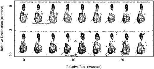
43 GHz (7 mm) VLBI maps of 3C 84 from 2015 May 11 (MJD 57153) until 2017 January 14 (MJD 57767). Contours: −1, 1, 2, 4, 8, 16, 32, 64 per cent of peak flux density. The emitting region used for the distance measurement is pointed out with a black arrow. The size and flux density is determined by Gaussian model-fitting the emitting region directly. The results of this fitting are found in Table 1. The flux densities obtained are used in the light curve shown in Fig. 2.
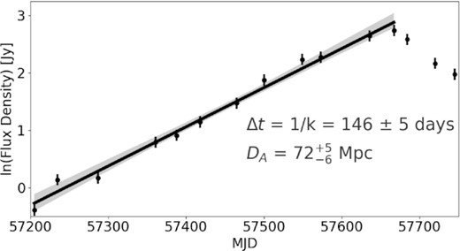
The light curve of the emitting region, as determined from directly model-fitting the maps is shown in Fig. 1. The variability time-scale is defined as the reciprocal of the slope, k, fit to the log of the flux densities between the minimum and maximum flux densities observed during a flare in the source. The solid black line is the best fit to the slope and the grey shaded area is the 95 per cent confidence interval. Assuming that this variability is reasonably constrained by the speed of light, this provides an estimate of the linear size of the emitting region. This is compared with the angular radius of the emitting region measured using VLBI (θVLBI = 0.20 ± 0.02 mas) in order to determine a angular diameter distance of |$D_{\mathrm{ A}} = 72^{+5}_{-6}$| Mpc.
Table of Gaussian model-fitted values used in this paper.
| MJD | Flux density | Half FWHM | Beam (maj |$\times$| min, PA) |
|---|---|---|---|
| (Jy) | (mas) | (mas |$\times$| mas), (°) | |
| 57205 | 0.67 ± 0.07 | 0.16 ± 0.01 | 0.160 |$\times$| 0.337, 5.27 |
| 57235 | 1.14 ± 0.15 | 0.29 ± 0.02 | 0.154 |$\times$| 0.280, 7.87 |
| 57287 | 1.18 ± 0.18 | 0.07 ± 0.01 | 0.166 |$\times$| 0.311, 3.49 |
| 57361 | 2.21 ± 0.22 | 0.11 ± 0.01 | 0.169 |$\times$| 0.276, 6.01 |
| 57388 | 2.48 ± 0.25 | 0.08 ± 0.01 | 0.168 |$\times$| 0.327, 7.48 |
| 57418 | 3.14 ± 0.31 | 0.08 ± 0.01 | 0.158 |$\times$| 0.281, 4.73 |
| 57465 | 4.36 ± 0.44 | 0.07 ± 0.01 | 0.162 |$\times$| 0.314, 3.16 |
| 57500 | 6.53 ± 0.65 | 0.18 ± 0.02 | 0.158 |$\times$| 0.278, 5.67 |
| 57549 | 9.33 ± 0.93 | 0.22 ± 0.02 | 0.164 |$\times$| 0.314, 15.90 |
| 57573 | 9.73 ± 0.97 | 0.20 ± 0.02 | 0.161 |$\times$| 0.302, 13.91 |
| 57636 | 14.06 ± 1.44 | 0.18 ± 0.01 | 0.160 |$\times$| 0.312, 1.50 |
| 57667 | 15.68 ± 1.53 | 0.20 ± 0.02 | 0.185 |$\times$| 0.423, 24.24 |
| 57684 | 13.25 ± 1.64 | 0.21 ± 0.02 | 0.161 |$\times$| 0.295, 13.97 |
| 57720 | 8.73 ± 0.87 | 0.23 ± 0.02 | 0.161 |$\times$| 0.300, 5.75 |
| 57745 | 7.21 ± 0.72 | 0.20 ± 0.02 | 0.160 |$\times$| 0.289, 7.82 |
4 RESULTS
The VLBI morphology of the source is currently dominated by two main emitting regions: the region thought to be near the central SMBH, which is the northernmost bright emission region in the maps shown in Fig. 1, and a slowly moving emission feature to the south and which has been studied recently by several authors (Nagai et al. 2016; Hiura et al. 2018; Hodgson et al. 2018). The slowly moving emission feature had a large flare occur in it, beginning in mid-2015, which is pointed out with black arrows (Hodgson et al. 2018). It should be noted that the relevant quantity is not the relative motion of the emission region from the SMBH but its flux density and size. We use this flare and directly model-fit it (acquiring the size and flux density information of the emitting region directly) to perform our distance measurements. The critical epochs are the beginning and peak of a flare. We discuss this in the next paragraph. In order to determine the variability (light-crossing, Δt) time-scale, we fit the slope, k, to the logarithmic flux density (ln S) as a function of time (modified Julian date, MJD) in a range of flux density from Smin to Smax (see Fig. 2). We determined Smin to be the first epoch in which the emission region was reliably detected in the VLBI images. See Appendix A for a more in-depth discussion. The variability time-scale is then 1/k (i.e. the e-folding time-scale of the flare), which is a standard method in the literature (Terasranta & Valtaoja 1994; Valtaoja et al. 1999; Jorstad et al. 2005; Hovatta et al. 2009; Jorstad et al. 2017). We determined a variability time-scale of Δt = 145 ± 5 d. The radius of the FWHM fitted to the emitting region at the peak of the flare is measured to be θVLBI = 0.20 ± 0.02 mas, with the component being easily resolved by the interferometer. We measure the size at the peak of the flare. This is because if one imagines a photon travelling across the source at the speed of light, it would necessarily be at least restricted to the size that we measure at the peak, since a photon would have had to travel at least that distance in order to make the size that we measure.
4.1 Error analysis
Errors were propagated using a Monte Carlo approach by creating a normal distribution for each observable. The mean of the distribution was set as the observed value and the standard deviation of the distribution was set as the error on the observed value. A distribution made of 10 000 samples was made for each variable and these distributions were used in the place of the variables presented in the equations shown in this paper. The 1σ final errors were determined by finding the 68 per cent limits of the final distribution. This leads to an estimate for the angular diameter distance of |$D_{\mathrm{ A}} = 72^{+5}_{-6}$| Mpc (corresponding to a Hubble constant of |$H_{0}=73^{+5}_{-6}$| km s−1 Mpc−1).
4.2 Sources of systematic error
A major source of systematic errors can come from the observations themselves. A limitation of the results presented here is that we are highly cadence and resolution limited using existing telescopes and monitoring programmes. These data were observed with a roughly monthly cadence. It is possible that there are flares that are shorter than a month in duration, that are missed due to the limited cadence of the observations. Similarly, we may not measure the correct size due to not observing exactly at the peak of a flare. VLBI flux density calibration can be somewhat uncertain and include flux-scaling errors. This can require comparison with total-intensity measurements (e.g. Kim et al. 2019) which could also lead to systematic errors. While angular resolution is not a problem with these observations, if we observe at high redshift, it could be possible that the source becomes unresolved. In this case, we could place limits on the size of the emitting region by using the major and minor axes of the observing beam (Gurvits et al. 1999; Cao et al. 2015). Furthermore, the results obtained here were achieved at an observing frequency of 43 GHz. According to AGN jet models (e.g. Blandford & Königl 1979; Bloom & Marscher 1996), the variability time-scale is expected to vary as a function of frequency. We, therefore, suggest continued observations at both higher and lower frequencies to further verify our methods. Nevertheless, even with perfect observations, there are several other potential sources of systematic errors. They include (i) the assumption that the variability is constrained by the speed of light; (ii) uncertainties in the geometry of the emission region; and (iii) determining when a flare begins and ends. (i) The key assumption of the method is that the observed variability is reasonably constrained by the speed of light. On a physical level, the emission from 3C 84 is due to synchrotron radiation by electrons (or other charged particles) being accelerated around magnetic field lines travelling at nearly the speed of light. Given the physics of the radiation, we believe it likely that the emission is tightly constrained by the speed of light, but not exactly. This assumption has been indirectly investigated by Liodakis & Pavlidou (2015) and Liodakis et al. (2018). In these studies, they investigated different methods for determining the Doppler factor in a large sample of AGN. They found that the variability Doppler factor – which depends on the causality assumption – best-fits the population. Implicitly this suggests that the causality assumption is valid. However, the results of Liodakis & Pavlidou (2015) are model dependent, because it assumes a source distribution model. Additionally, a way to directly test the assumption would be to use this method on microquasars with known parallax distances (e.g. Reid et al. 2014). We intend to perform these observations in the future. (ii) There is also some uncertainty regarding the geometry of the emission region. In this proof-of-concept paper, we are unable to differentiate between a spherical geometry, a thin-disc geometry or non-face-on orientations of thin disc geometries or more complex geometries (e.g. Protheroe 2002). However with careful analysis of the visibilities of sufficiently high resolution observations, it should be possible to determine the true source geometry (Pearson 1995). Furthermore, we assume that the variability time-scale equates to the radius of the emitting region, and that we are sensitive to the longest axis of a project ellipsoid. Given that the emitting regions are likely shock-fronts, we believe this to be a reasonable assumption. However with a careful analysis of visibilities in simple sources, this can be accounted for or potentially also modelled. (iii) Determining the variability time-scale is a critical parameter in deriving distances, with the critical parameters being when a flare begins and ends. This is discussed in Appendix A. Some potential ways to correct for uncertainties in the variability time-scale could be to use γ-ray flaring as a proxy for a flare onset or using polarization measurements. In the case of 3C 84, we are nevertheless confident that we are reasonably accurately measuring the variability time-scale, as the distance we derive is consistent with other methods. In particular, the presence of a type Ia supernova in the galaxy allows a distance measurement of 62.5–82.8 Mpc (Hicken et al. 2009), while Tully–Fisher measurements to the brightest galaxy yield a distance of 53.9–68.9 Mpc (Theureau et al. 2007). We should emphasize that systematic errors such as these should not have any redshift dependence. This means that these errors can affect the absolute scaling of the distance measurements, but not the shape as a function redshift. Therefore, this can affect measurements of the Hubble Constant, but should not affect measurements of the energy content of the universe. However, quasars and blazars exhibit relativistic effects that must be taken into account in order to determine accurate distances at the highest redshifts. In an upcoming paper, we will investigate other sources and demonstrate how these relativistic effects can be accounted for and therefore applied to a larger range of sources, and potentially bridging the gap between supernova and CMB measurements. However, for strongly relativistic sources, there could be redshift-dependent systematic errors. This could arise from a selection bias, where we preferentially select only the most relativistic sources at the highest redshifts. How an effect like this would manifest itself in practice is not yet clear. For radio galaxies which are only mildly relativistic, we can apply our method directly.
5 CONCLUSIONS
We have presented a proof-of-concept measurement of an angular diameter distance that is independent of cosmological model assumptions and of the distance ladder. It is worth noting that this method can also be applied to non-AGN-type sources. In order for our method to work, a source need only have its flux density variability reasonably approximated by the speed of light and be resolvable by our instruments. In order to perform these observations, cadence and high-resolution monitoring will be required. Within this context, there are currently plans to convert the Mopra telescope in Australia to be compatible with the quasi-optics of the Korean VLBI Network. The KVN is capable of observing at four frequencies simultaneously (Lee et al. 2014; Hodgson et al. 2016), allowing us to confirm that the variability time-scales and sizes change as a function of frequency. We will be able to perform multifrequency, high-cadence, and high-resolution monitoring of AGNs over a large range of redshifts, allowing us to constrain both the Hubble constant and the matter density of our Universe.
ACKNOWLEDGEMENTS
The author would like to acknowledge the help of Alan Marscher and Svetlana Jorstad for their help in preparing this manuscript and providing the data for 3C 84. This work by Jeffrey A. Hodgson was supported by Korea Research Fellowship Program through the National Research Foundation of Korea (NRF) funded by the Ministry of Science and ICT (2018H1D3A1A02032824). This study makes use of 43 GHz VLBA data from the VLBA-BU Blazar Monitoring Program (VLBA-BU-BLAZAR; http://www.bu.edu/blazars/VLBAproject.html), funded by NASA through Fermi Guest Investigator grant 80NSSC17K0649. The VLBA is an instrument of the National Radio Astronomy Observatory. BL would like to acknowledge the support of the National Research Foundation of Korea (NRF-2019R1I1A1A01063740). This work was supported by the Samsung Science and Technology Foundation under Project Number SSTF-BA1801-04.
Footnotes
Maps available from https://www.bu.edu/blazars/VLBA_GLAST/0316.html
REFERENCES
APPENDIX A:
DETERMINING THE VARIABILITY TIME-SCALE
Accurately determining the variability time-scale (Δt) is of critical importance for determining the distance, with it being sensitive to determining the onset of the flare. In this case, we consider the flare to begin in the first epoch that the flaring component was reliably detected in the VLBI images. Furthermore, a very bright γ-ray flare has been associated with the emergence of this component (Hodgson et al. 2018), with it peaking in 2015.81 (MJD 57318), although its onset is approximately 2015.6–2015.7 (MJD 57240–57280), which is consistent with the emergence of the component. Nevertheless, we can explore how the distance measurement is affected by different flare definitions. In Fig. 2, we can see that the flux density slightly decreases at ∼MJD 57300. If we select this epoch as when the flare begins, we derive a distance of |$D_{\mathrm{ A}}=70^{+6}_{-6}$| Mpc, which makes a ∼1 per cent difference and is still consistent with distances measured using other methods (Theureau et al. 2007; Hicken et al. 2009). We plan to fully investigate the most appropriate way to determine the variability time-scales in our upcoming project.
