


Abstract
We report the first analytical expression purely constructed by a machine to determine photometric redshifts (zphot) of galaxies. A simple and reliable functional form is derived using 41 214 galaxies from the Sloan Digital Sky Survey Data Release 10 (SDSS-DR10) spectroscopic sample. The method automatically dropped the u and z bands, relying only on g, r and i for the final solution. Applying this expression to other 1417 181 SDSS-DR10 galaxies, with measured spectroscopic redshifts (zspec), we achieved a mean 〈(zphot − zspec)/(1 + zspec)〉 ≲ 0.0086 and a scatter σ(zphot − zspec)/(1 + zspec) ≲ 0.045 when averaged up to z ≲ 1.0. The method was also applied to the PHAT0 data set, confirming the competitiveness of our results when faced with other methods from the literature. This is the first use of symbolic regression in cosmology, representing a leap forward in astronomy-data-mining connection.
1 INTRODUCTION
A novel methodology was recently proposed to automatically search for underlying analytical laws in data (Schmidt & Lipson 2009). Its importance has been highlighted in astronomy by Graham et al. (2013), and this Letter is the first attempt to use it in a cosmological context. We applied the aforementioned method to derive an analytic expression for photometric redshift (photo-z) determination from Sloan Digital Sky Survey 10th data release (SDSS-DR10, Ahn et al. 2014) spectroscopic sample of galaxies. Our goal here is to demonstrate the potential of machine proposed analytical relations in providing simple and reliable photo-z.
Due to the variety of spectra occurring in nature (as there are several types of galaxies of different ages, metalicities, star-forming histories, merging histories, etc.), the unicity of photometric redshift estimates is not assured for any sample. Nevertheless, the large amount of data expected to be observed by surveys like the Large Synoptic Survey Telescope1 (LSST Science Collaboration: Abell et al. 2009), Euclid2 (Refregier et al. 2010) or Wide-Field Infrared Survey Telescope3 (Green et al. 2012) makes it infeasible to obtain spectroscopic redshifts for all their objects with the current and likely near future technology. Therefore, making photo-z is the only viable solution for estimating redshifts in such large scale.
Photo-z methods have been widely used in fields as diverse as gravitational lensing (e.g. Mandelbaum et al. 2008; Zitrin et al. 2011; Nusser, Branchini & Feix 2013), baryon acoustic oscillations (e.g. Nishizawa, Oguri & Takada 2013), quasars (e.g. Richards et al. 2009), luminous red galaxies (LRGs; de Simoni et al. 2013) and supernovae (e.g. Kessler et al. 2010). At the same time, numerous efforts to accurately determine photo-z were reported (for a glimpse on the diversity of existent methods, see Hildebrandt et al. 2010; Abdalla et al. 2011; Zheng & Zhang 2012, and references therein). To deepen our understanding of the differences between photo-z techniques, Abdalla et al. (2011) compared results from six methods applied to LRGs. They show 1σ scatters between 0.057 and 0.097 when averaged over the considered redshift range (0.3 ≤ z ≤ 0.8), systematically presenting poor accuracy at low (z ≤ 0.4) and high (z ≥ 0.7) redshifts. More recently, Hildebrandt et al. (2010) presented a wider comparison enclosing 16 different methods. The methods perform better in simulated than real data, with empirical codes showing smaller biases than template-fitting ones.
The existing approaches are usually divided in two classes: empirical (e.g. Connolly et al. 1995; Collister & Lahav 2004; Wadadekar 2005; Miles, Freitas & Serjeant 2007; O'Mill et al. 2011; Reis et al. 2012; Carrasco Kind & Brunner 2013) and template-fitting-based methods (e.g. Benítez 2000; Bolzonella, Miralles & Pelló 2000; Ilbert et al. 2006). The former uses magnitudes and/or colours of a spectroscopically measured sample for training the method, which is then applied to the photometric sample. The latter, try to find spectral template and redshift which best fit the photometric observations using a library of well known observational or synthetic spectra.
The main advantage of the approach adopted in this Letter is that without any a priori physical information nor ad hoc functional form, it empirically derives analytical expressions from the data. Besides that, the error propagation from the observables can be straightforwardly performed into the redshift estimate. Also, due to its analytic nature, the outcomes are more tractable, and thus interpretable, than the outcomes of other methods, such as neural networks or support vector machines, for instance. Finally, the resulting expressions are promptly portable, and might even be incorporated on the fly via Structured Query Language (sql) when retrieving catalogue data, for instance.
The outline of this Letter is as follows. In Section 2, we give a broad picture of the methodology followed in this Letter. Then, Section 3 provides an overview of the adopted data set. Afterwards, we present our results and compare with the recent literature in Section 4. Finally, conclusions are presented in Section 5.
2 METHODOLOGY
The ultimate goal of symbolic regression-based techniques is to find a functional form that explains hidden associations in data sets, while optimizing a given error metric (e.g. Schmidt & Lipson 2009). This is fundamentally distinct from linear and non-linear regression methods that fit parameters for an a priori analytical expression. In symbolic regression, the machine searches the best expression and the optimal coefficients simultaneously.
We used the software eureqa4 (Schmidt & Lipson 2009) to test the application of symbolic regression for photo-z determination. It allows the user to choose atomic function blocks (basic mathematical operations, exponentials, logarithms, boolean operators, trigonometric functions, etc.). Then, eureqa scans through the data and a variety of combinations between the atomic function blocks are evolved through genetic programming (Koza 1992), optimizing conciseness and accuracy. Lastly, the outcome functions are ordered according to their complexity and quality of the fit.
The application of eureqa to our problem follows a straightforward approach. First, a subset of galaxies with measured spectroscopic redshifts is used to derive an analytical expression that optimally predicts the redshift from the magnitude and colour data. In other words, an expression whose evaluation minimizes the mean absolute error when compared to the data. To seek simplicity while keeping accuracy, we only allowed the use of simple mathematical operations (+, −, *, /). Afterwards, the obtained expression is applied to a larger sample of galaxies with spectroscopic measurements, to perform a strict validation of the expression's predictive capability against real spectroscopic redshifts.
3 DATA
The data adopted in this work were selected from the SDSS-DR10 spectroscopic sample. This includes hundreds of thousands of new galaxies and quasar spectra from the Baryon Oscillation Spectroscopic Survey5 in addition to all imaging and spectra from prior SDSS data releases.
From this data set, we selected all objects with spectroscopic measurements (table SpecObj) classified as galaxies (flag SpecObj.class = ‘GALAXY’) and whose spectra were free from known problems (flag SpecObj.zWarning = 0). Moreover, only sources with clean photometric measurements (flag PhotoObj.CLEAN = 1) were accepted. The sql query used in SDSS CasJobs6 service was:
SELECT s.specObjID, g.u, g.g, g.r, g.i, g.z,
s.z AS redshift
INTO mydb.specObjAllz_cleanphoto
FROM SpecObj AS s JOIN Galaxy AS g
ON s.specobjid = g.specobjid, PhotoObj
WHERE class = 'GALAXY' AND zWarning = 0
AND g.objId = PhotoObj.ObjID
AND PhotoObj.CLEAN=1
where s.specObjID is the object identification in the spectral tables and g.u, g.g, g.r, g.i, g.z, s.z represent the SDSS's ugriz model magnitudes and measured spectroscopic redshift, respectively. This resulted in a data set containing 1458 404 objects, from which we retained only galaxies with zspec < 1.0. Additionally, all possible colour combinations based on the available photometric bands were computed.
We divided the data into two subsets, one for deriving the analytic expression and another for validation and error assessment. To mitigate biases created by unbalanced data, we randomly selected 5000 galaxies per redshift bin (width Δzspec = 0.1) up to zspec = 0.8. For 0.8 ≤ zspec < 1.0, half of all available objects in each redshift bin were used for deriving the expression. This comprises a total of 41 214 galaxies that were used for searching the expression. Then, the accuracy (systematic errors) and precision (random errors) of this expression were assessed based on other 1417 181 objects. We only considered objects with zspec > 0.
Finally, we did not apply any cuts in magnitude, quality of spectroscopic redshift measurement nor galaxy types. This ensures that our results are not biased towards high signal-to-noise data, a particular galaxy type nor optimal observation conditions in comparison with the SDSS-DR10 spectroscopic sample.
4 RESULTS
This represents a rather simple empirical relation between photometric measurements and redshifts of galaxies calibrated for the SDSS-DR10 spectroscopic sample.7 Given its analytical nature, equation (1) allows a straightforward error propagation from the uncertainties in the measured magnitudes to the final photometric redshift. Note the missing u and z bands in the former equation. Such behaviour was observed in several equations constructed by eureqa, suggesting that a competitive performance might be reached using only three SDSS photometric bands.8
Interestingly, the two SDSS filters kept out of the derived equation are those which do not bracket the main spectral feature for imprinting redshift signature in photometry, for the redshift range considered in this work: the ∼4000 Å break. This does not mean that these filters carry null information. Instead, it only highlights that the bulk of information relevant to photometric redshift determination relies on the other filters. Due to a compromise between error and complexity during the optimization procedure, only the most relevant filters survive to the output equations. Moreover, the expressions assembled by eureqa are not simply high-order polynomials with additional terms, but more intricate combinations of magnitudes in different filters. Accordingly, expressions with more terms are not necessarily expected to improve redshift estimates, as additional terms might even introduce degeneracies.
To test the performance of equation (1), we applied it to the photometric data of 1417 181 galaxies. Fig. 1 summarizes our results, showing a comparison between zspec and zphot. One can promptly notice that zspec is well recovered by zphot with reasonable accuracy. Furthermore, a reasonable match between zspec and zphot distributions can be observed (upper and right-hand panels, respectively). This indicates that equation (1) recovers the underlying redshift distribution over a significant fraction of the explored redshift range.
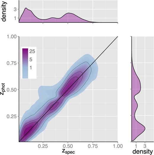
Kernel density distribution of photometric (zphot) versus spectroscopic (zspec) redshifts for more than one million SDSS-DR10 galaxies. The colour scale is logarithm, so a difference of 1 is equivalent to a density variation by a factor of e. Distributions for zspec and zphot redshifts are shown on the top and right-hand panels.
The left-hand panel of Fig. 2 shows the probability distribution functions (PDF) of (zphot − zspec)/(1 + zspec) in each redshift bin (width Δzspec = 0.1) for 0 ≤ zspec < 1.0, represented as violin plots. Each ‘violin’ centre represents the median of the distribution, while the shape its the mirrored PDF. The drop in medians at high redshifts (zspec ≳ 0.7) indicates that zphot systematically underestimates zspec at this range. This might be caused by poor statistics: in the full data set, at zspec ≥ 0.8 there are only 2428 objects, while for zspec ≥ 0.7 there are 25 439. This underweighs the contribution of high-z objects to the construction of equation (1). Accordingly, for bins with equally balanced number of galaxies (zspec ≤ 0.7), no obvious systematic effects are seen.
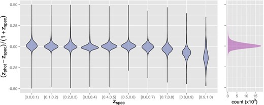
Left-hand panel shows the photometric redshift error distributions estimated from equation (1), in redshift bins of width Δzspec = 0.1. Right-hand panel displays the error distribution for more than one million galaxies in SDSS-DR10 as a histogram with bins of width Δ((zphot − zspec)/(1 + zspec)) = 0.001.
The right-hand panel of Fig. 2 shows a histogram of (zphot − zspec)/(1 + zspec), with bins of 0.001, forming a nearly perfect normal error distribution. As the mean and standard deviation are known to be sensitive to outliers, we removed the extreme tails of zphot distribution prior to computing them (117 events, or less than 0.008 per cent of the sample). This rejection is performed directly in the zphot distribution without any prior knowledge about zspec. The mean is 〈(zphot − zspec)/(1 + zspec)〉 ≈ 0.0086, while the scatter is |$\sigma _{(z_{\rm phot}-z_{\rm spec})/(1+z_{\rm spec})} \approx 0.0449$|.9 Albeit using a different data set, Hildebrandt et al. (2010) obtained similar values (0.005 ≤ |〈(zphot − zspec)/(1 + zspec)〉| ≤ 0.039 and |$0.034 \le \sigma _(z_{\rm phot}-z_{\rm spec})/(1+z_{\rm spec}) \le 0.076$|). Nevertheless, given the different adopted data sets, we refrain from performing a direct comparison with our results. Notwithstanding, these figures suggest that equations derived by eureqa might be competitive against more elaborated methods.
Using a homogeneous sample of LRGs, Abdalla et al. (2011) tested six different methods, reporting 0.0014 ≤ |〈zphot − zspec〉| ≤ 0.0302 and |$0.0575 \le \sigma _{(z_{{\rm phot}}-z_{{\rm spec}})} \le 0.0973$|. These values are compatible with those obtained by equation (1), 〈zphot − zspec〉 ≈ 0.0104, with a scatter10 of |$\sigma _{(z_{{\rm phot}}-z_{{\rm spec}})} \approx 0.0570$|. This reinforces the relevance of results achieved by the analytical expression derived with eureqa. Despite its simple nature, it was able to deliver competitive accuracy and precision from a rather diverse and inhomogeneous sample.
To estimate the level of bias introduced by equation (1) into a given cosmological inference, it is necessary to discuss the number of catastrophic errors, i.e. cases when photo-z is above a given tolerance threshold (Bernstein & Huterer 2010). These authors consider catastrophic errors as |zphot − zspec| ≳ 1, while Hildebrandt et al. (2010) defined them as |zphot − zspec| > 0.15(1 + zspec) or >0.5. Molino et al. (2014) consider redshift-dependent limits in terms of median and MAD, which in our context means |zphot − zspec| ≥ 0.2 at z = 0 and 0.39 at z = 1.0. Fig. 3 shows the catastrophic error rate obtained from equation (1) as a function of zspec for three different scenarios: |zphot − zspec| > 0.1, 0.25 and 0.5. The choice of three independent criteria gives a glimpse of how equation (1) performs in a wide range of accuracy requirements. In each panel, the bar plots are given in logarithm scale, where face-down bars indicate less than 1 per cent of catastrophic errors according to the criteria on the right.
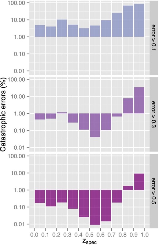
Percentual of catastrophic errors resulting from the photo-z estimation at each redshift bin for three different scenarios: |zphot − zspec| > 0.1, 0.3 and 0.5, from top to bottom.
5 CONCLUSIONS
This work is the first attempt to use a heuristic machine assistant to propose new analytical relationships for photo-z estimation. It provides a simple and accurate functional form based on photometric information of SDSS spectroscopic sample galaxies. Although we started the search using all five SDSS bands, several solutions relied only on three of them. Hence, showing that for SDSS bands, a competitive performance can be attained even with a moderate number of filters.
We adopted a set of 41 214 galaxies for determining the photo-z expression. Afterwards, it was used to estimate zphot for another 1417 181 galaxies with known zspec. Our results achieved 〈(zphot − zspec)/(1 + zspec)〉 ≲ 0.0086 and a scatter |$\sigma _{(z_{\rm phot} - z_{\rm spec})/(1+z_{\rm spec})}\lesssim 0.045$| when averaged up to z ≲ 1.0. These results indicate that symbolic regression is competitive against other methods available in the literature. An inspection of the (zphot − zspec)/(1 + zspec) distributions per redshift bin reveals systematic effects at zspec ≳ 0.7. Such behaviour might be caused by the poor statistics at high redshifts.
The conciseness of the outcomes obtained by eureqa is stressed by how easily they can be adopted by the astronomical community. The functions can even be directly incorporated into simple sql queries. Such level of portability is unattainable by the majority of photo-z methods currently available (but see e.g. Connolly et al. 1995; Hsieh et al. 2005). Moreover, the error propagation can be straightforwardly achieved by deriving the redshift as a function of photometric observables (e.g. Collister & Lahav 2004; Oyaizu et al. 2008).
Finally, the possibility to use computers to unveil hidden analytical relationships in data sets, a heretofore task exclusive of humans, is astonishing (e.g. Schmidt & Lipson 2009; Graham et al. 2013). Astronomy is already being flooded by an unprecedented amount of data, and this tendency is expected to increase even more in the next decade. Therefore, the possibility to connect these novel systems to data bases, and particularly allowing them to perform text mining in scientific literature (as in Leach et al. 2009), might represent a new paradigm for astronomical exploration. These methods are coming to stay, and although still incipient and naive, they host a great potential to help humankind in its endeavour to unravel the Universe.
We thank Reinaldo Ramos de Carvalho, Andressa Jendreieck, Laerte Sodré Jr, Filipe Abdalla, Jon Loveday, Matias Carrasco, Jonatan D. Hernandez Fernandez and Ana Laura O'Mill for interesting suggestions and comments. EEOI and RSS thank the SIM Laboratory of the Universidade de Lisboa for hospitality during the development of this work. This work was partially supported by the ESA VA4D project (AO 1-6740/11/F/MOS). AKM thanks the Portuguese agency Fundação para Ciência e Tecnologia, FCT, for financial support (SFRH/BPD/74697/2010). EEOI thanks the Brazilian agencies FAPESP (2011/09525-3) and CAPES (9229-13-2) for financial support. Funding for SDSS-III has been provided by the Alfred P. Sloan Foundation, the Participating Institutions, the National Science Foundation and the US Department of Energy Office of Science. The SDSS-III website is http://www.sdss3.org/. This work was written on the collaborative sharelatex platform.
We stress that this expression was calibrated for the SDSS-DR10 spectroscopic sample, and should not be extrapolated out of this scope.
A more robust statistical estimator against outliers are the median and median absolute deviation values (MAD). For this data set, we obtained a median of 0.0048 and MAD = 0.0318.
Using robust statistics, we obtain a median of 0.0062 and MAD = 0.0414.
REFERENCES
APPENDIX A: COMPARISON OTHER METHODS
To compare symbolic regression with other methods and better situate our results, we adopted a publicly available data set that was previously submitted to different photo-z codes. The PHoto-z Accuracy Testing (PHAT) was an international initiative to identify the most promising photo-z methods and guide future improvements. Two observational photometric catalogues were provided: PHAT0 with simulations and PHAT1 with real observations. A total of 17 photo-z codes were submitted. As a direct comparison using PHAT1 is not possible, as the answers of the challenge are not openly available, we applied symbolic regression to PHAT0 and compared its results to those reported by Hildebrandt et al. (2010).
This expression, when applied to the validation data set, yields 〈(zphot − zspec)/(1 + zspec)〉 = 0.001, |$\sigma _{(z_{\rm phot} - z_{\rm spec})/(1+z_{\rm spec})} = 0.039$| and an outlier fraction of 4.331 per cent. Here, we report the outlier fraction as |zphot − zspec| > 0.15(1 + zspec), according to the definition adopted by Hildebrandt et al. (2010). Results for all 17 photo-z codes submitted to PHAT for the PHAT0 data set can be summarized as −0.05 ≤ (zphot − zspec)/(1 + zspec) ≤ 0.001, |$0.010 \le \sigma _{(z_{\rm phot} - z_{\rm spec})/(1+z_{\rm spec})} \le 0.049$| and outlier fraction between 0.010 per cent and 18.202 per cent. Comparing these results, we confirm that the accuracy of our results are within the values reported by other widely used methods.
Finally, Fig. 4 shows the error distributions per redshift bin. Most of the data used to derive the expression (≈99.5 per cent) are concentrated at z ≤ 1.45, which not surprisingly corresponds to the interval where the photo-z determination is more accurate. On the other hand, the expression shows a degraded performance at higher redshifts (which contain less than ≈0.5 per cent of the data). This is similar to the results found for the SDSS-DR10 sample, indicating that in cases where a homogeneous data distribution is available, the symbolic regression results are competitive to available methods.
SUPPORTING INFORMATION
Additional Supporting Information may be found in the online version of this article:
Figure 4. Left-hand panel shows the photometric redshift error distributions for the PHAT0 data set and equation (A1) in redshift bins of width Δzspec = 0.2 in the range |$[0 \text{--} 2.2)$|. Right-hand panel displays the error distribution of all the galaxies (bins of width Δ((zphot − zspec)/(1 + zspec)) = 0.001) (http://mnrasl.oxfordjournals.org/lookup/suppl/doi:10.1093/mnrasl/slu067/-/DC1).
Please note: Oxford University Press is not responsible for the content or functionality of any supporting materials supplied by the authors. Any queries (other than missing material) should be directed to the corresponding author for the paper.
