


ABSTRACT
Recent work has suggested that, during reionization, spatial variations in the ionizing radiation field should produce enhanced Ly |$\alpha$| forest transmission at distances of tens of comoving Mpc from high-redshift galaxies. We demonstrate that the Sherwood–Relics suite of hybrid radiation-hydrodynamical simulations are qualitatively consistent with this interpretation. The shape of the galaxy–Ly |$\alpha$| transmission cross-correlation is sensitive to both the mass of the haloes hosting the galaxies and the volume averaged fraction of neutral hydrogen in the IGM, |$\bar{x}_{\rm H\,I}$|. The reported excess Ly |$\alpha$| forest transmission on scales |$r \sim 10~{\rm cMpc}$| at |$\langle z \rangle \approx 5.2$| – as measured using C iv absorbers as proxies for high-redshift galaxies – is quantitatively reproduced by Sherwood–Relics at |$z=6$| if we assume the galaxies that produce ionizing photons are hosted in haloes with mass |$M_{\rm h}\ge 10^{10}~h^{-1}\, {\rm M}_\odot$|. However, this redshift mismatch is equivalent to requiring |$\bar{x}_{\rm H\,I}\sim 0.1$| at |$z\simeq 5.2$|, which is inconsistent with the observed Ly |$\alpha$| forest effective optical depth distribution. We suggest this tension may be partly resolved if the minimum C iv absorber host halo mass at |$z>5$| is larger than |$M_{\rm h}=10^{10}~h^{-1}\, {\rm M}_\odot$|. After reionization completes, relic IGM temperature fluctuations will continue to influence the shape of the cross-correlation on scales of a few comoving Mpc at |$4 \le z \le 5$|. Constraining the redshift evolution of the cross-correlation over this period may therefore provide further insight into the timing of reionization.
1 INTRODUCTION
Between the first hundred million years and the first billion years, the hydrogen gas permeating the Universe transitioned from cold and neutral to warm and (re)ionized. A wide variety of observational constraints place the mid-point of reionization between |$7 \lesssim z \lesssim 8$| (e.g. Bañados et al. 2018; Davies et al. 2018; Greig, Mesinger & Bañados 2019; Jung et al. 2020; Planck Collaboration VI 2020; Gaikwad et al. 2023; Jin et al. 2023; Ďurovčíková et al. 2024; Umeda et al. 2024). The rapid evolution of the mean free path of Lyman-limit photons between |$5< z < 6$| (Becker et al. 2021; Zhu et al. 2023; Satyavolu et al. 2024), the distribution of the Ly |$\alpha$| forest transmission (Bosman et al. 2022), and the presence of damping wings in the spectra of |$z< 6$| quasars (Becker et al. 2024; Spina et al. 2024; Zhu et al. 2024a) are furthermore consistent with the last neutral hydrogen islands persisting to |$z < 6$|. This suggests reionization may have finished around |$z \approx 5.3$| (Kulkarni et al. 2019; Keating et al. 2020a, b; Nasir & D’Aloisio 2020).
Concurrently, JWST is opening up a new window on galaxy formation at |$z \gtrsim 8$| (e.g. Naidu et al. 2022; Arrabal Haro et al. 2023; Castellano et al. 2024; Harikane et al. 2024; Zavala et al. 2025). Constraints from deep observations with JWST suggest that faint, low-mass galaxies are efficient at producing ionizing photons, and can provide the majority of the ionizing photons required for reionization (Atek et al. 2024; Begley et al. 2024; Saxena et al. 2024; Simmonds et al. 2024, although see also Gazagnes et al. 2024). The discovery of many faint active galactic nuclei (AGNs; e.g. Harikane et al. 2023) also means that a contribution to the ionizing photon budget by faint AGNs is plausible (Asthana et al. 2024a; Grazian et al. 2024; Madau et al. 2024; Maiolino et al. 2024).
A promising route for connecting the properties of the IGM with these high-redshift ionizing sources is a cross-correlation with intergalactic Ly |$\alpha$| transmission. At low redshifts (|$z< 5$|), well after the end of reionization, the galaxy–Ly |$\alpha$| transmission correlation has been extensively studied (Adelberger et al. 2005; Tummuangpak et al. 2014; Turner et al. 2014; Bielby et al. 2017; Banerjee et al. 2024; Matthee et al. 2024). The low-redshift (|$2\lesssim z \lesssim 4$|) picture that has emerged is one of a strong decrease in Ly |$\alpha$| transmission approaching galaxies, driven by enhanced overdensities and the clustering and infall of neutral hydrogen in the regions where these galaxies reside. Models of this low-redshift deficit in transmission at small impact parameters (|$b\lesssim 1~{\rm cMpc}$|) also suggest that stellar feedback plays an important role in setting the level of Ly |$\alpha$| transmission (Meiksin, Bolton & Puchwein 2017; Sorini, Davé & Anglés-Alcázar 2020).
At higher redshifts, the picture is less clear. Kakiichi et al. (2018) used a small sample of spectroscopically confirmed Lyman break galaxies (LBGs) at |$5.3 < z < 6.4$| in the field of a |$z=6.42$| quasi-stellar object (QSO) to examine the impact of local ionization on Ly |$\alpha$| transmission. They cross-correlated the positions of these LBGs with the Ly |$\alpha$| forest, finding that there was some evidence (tempered by the small sample size) for an enhancement of Ly |$\alpha$| transmission in proximity to galaxies. This enhancement they attributed not solely to the observed LBGs, but also to the ionizing radiation produced by nearby, faint, and therefore undetected, sources. Meyer et al. (2019) computed the 1D correlation between C iv absorbers and Ly |$\alpha$| transmission in the spectra of 25 QSOs at |$4.5 < z < 6.3$|, finding reduced transmission at |$r\lesssim 7~{\rm cMpc}$| [qualitatively similar to the low-redshift results discussed previously, though quantitatively the deficit in transmission in Meyer et al. (2019) is somewhat stronger] and statistically significant enhanced Ly |$\alpha$| transmission relative to the mean at distances of |$r\sim 15$|–|$45~{\rm cMpc}$|. In a follow-up work, Meyer et al. (2020) characterized the galaxy–Ly |$\alpha$| transmission correlation at |$z\sim 6$|, but were unable to reproduce the findings of Meyer et al. (2019), which they attribute to a small sample size and noise. Additionally, Kashino et al. (2023) reported a measurement of the galaxy–Ly |$\alpha$| transmission correlation from a single QSO sightline from the EIGER survey at |$5.3< z < 5.7$| and |$5.7< z < 6.14$|. Finally, while this work was being completed, measurements of the galaxy–Ly |$\alpha$| transmission correlation over the redshift range |$5.4 < z< 6.5$| from the JWST ASPIRE survey were released (Kakiichi et al. 2025). Using five QSO fields, these authors reported |$2\sigma$| evidence for excess Ly |$\alpha$| transmission on scales of 20–|$40\rm \, cMpc$| from [O iii] emitting galaxies at |$\langle z \rangle = 5.86$|.
Modelling of the high-redshift galaxy–Ly |$\alpha$| transmission correlation using reionization simulations has also returned a variety of results. Garaldi, Gnedin & Madau (2019) performed the first examination of the transmission correlation in the high-redshift context, using the CROC simulations of cosmic reionization (Gnedin 2014). Garaldi et al. (2019) compared the results of the CROC simulation to the Meyer et al. (2019) observational constraints, finding that their models show a reduction in transmission close to galaxies (in a similar fashion to the low-z observations) but do not reproduce the enhanced transmission at larger radii reported by Meyer et al. (2019). Zhu, Gnedin & Avestruz (2024b) performed a further analysis of the CROC simulations and confirmed the absence of an excess in transmission. In contrast, Garaldi et al. (2022) showed that, in the THESAN simulations (Kannan et al. 2022; Smith et al. 2022), the galaxy–Ly |$\alpha$| transmission correlation shows both reduced transmission close to galaxies and excess transmission at larger distances. This is qualitatively similar to Meyer et al. (2019), although good agreement with the Meyer et al. (2019) results occurs at a different (higher) redshift in the models. Garaldi et al. (2022) also demonstrated that, in the context of the THESAN model, the galaxy–Ly |$\alpha$| transmission correlation is largely independent of the source model when reionization history is accounted for (e.g. by comparing the correlation at fixed neutral fraction |$x_{\rm H\,I}$|, as opposed to fixed redshift). Recently, Garaldi & Bellscheidt (2024a) performed a deeper analysis of the galaxy–Ly |$\alpha$| transmission correlation in THESAN, focusing on its observability. They noted that the selection criteria for galaxies (e.g. C iv absorption, [O iii] flux) appears to have little impact on the correlation in their models.
In this context, we examine the galaxy–Ly |$\alpha$| transmission correlation in the Sherwood–Relics1 simulation suite (Puchwein et al. 2023). In this work, we focus on the high-redshift (|$z\ge 4.2$|) galaxy–Ly |$\alpha$| transmission correlation, at distances |$r\gtrsim {\rm few~cMpc}$| from galaxies. Sherwood–Relics has demonstrated excellent agreement with observations for a range of IGM properties at |$z\lesssim 6$| (see e.g. Gaikwad et al. 2020; Molaro et al. 2022; Feron et al. 2024). The simulations differ from other numerical models in several ways. First, they have been designed specifically for modelling the properties of the Ly |$\alpha$| forest at the tail end of reionization, making them ideal for investigating the galaxy–Ly |$\alpha$| transmission correlation at |$z\sim 6$|. Secondly, instead of full radiation-hydrodynamics, Sherwood–Relics uses a novel hybrid radiative transfer (RT) scheme (see Section 2.1) that captures the hydrodynamical response of the gas to the inhomogeneous photoheating and photoionization associated with reionization. This allows different reionization histories to be examined at relatively low computational cost.
The paper is structured as follows: In Section 2.1, we briefly describe the simulations used in this work, and in Section 2.2 we perform an initial examination of the Ly |$\alpha$| transmission around galaxies in our fiducial model to gain intuition. Next, in Section 3 we explore the galaxy–Ly |$\alpha$| transmission correlation in Sherwood–Relics, and in Section 4 we explore the effect of different modelling assumptions in an attempt to elucidate the physical origin of the galaxy–Ly |$\alpha$| transmission correlation, both during and after reionization. Finally, we conclude in Section 5. We assume a flat |$\Lambda$|cold dark matter cosmology with |$\Omega _\Lambda =0.692$|, |$\Omega _{\rm m}=0.308$|, |$\Omega _{\rm b}=0.0482$|, |$\sigma _8=0.829$|, |$n_\mathrm{ s}=0.961$| and |$h=0.678$| (Planck Collaboration XVI 2014). Unless otherwise specified, distance units are comoving (and may be explicitly specified as such by the prefix ‘c’).
2 MODELLING LY α TRANSMISSION
2.1 Sherwood–Relics simulations
The simulations used in this work form part of the Sherwood–Relics project (see Puchwein et al. 2023, for details). The Sherwood–Relics suite of simulations are a series of high-resolution cosmological hydrodynamical simulations performed using a modified version of p-gadget-3 (itself a modified version of gadget-2, described in Springel 2005). In this study, we use runs with box sizes of |$40~h^{-1}\, {\rm Mpc}$| (40-2048) and |$160~h^{-1}\, {\rm Mpc}$| (160-2048), each containing |$2 \times 2048^3$| particles. In addition, for testing the convergence of our results with mass resolution, we also employ variants of the |$40~h^{-1}\, {\rm Mpc}$| box that are identical to 40–2048, except they were run with |$2\times 1024^3$| (40-1024) and |$2\times 512^3$| particles (40-512). See Table 1 for a summary of the runs used in this work.
Overview of the Sherwood–Relics runs employed in this study (see also Puchwein et al. 2023). Listed in columns are the name used to refer to the run; linear comoving box size in |$h^{-1}\, {\rm cMpc}$| (|$L_{\rm box}$|); total initial number of dark matter and gas particles (|$N_{\rm part}$|); dark matter particle mass in |$h^{-1}\, {\rm M}_\odot$| (|$M_{\rm d}$|); gas particle mass in |$h^{-1}\, {\rm M}_\odot$| (|$M_{\rm g}$|); redshift at which the global volume-averaged neutral fraction drops below |$10^{-3}$| (|$z_{\rm r}$|); and the output redshifts for snapshots |$z_{\rm snap}$|. The lowest redshift snapshot for all models is |$z=4.2$|.
| Name | |$L_{\rm box}$| (|$h^{-1}\, {\rm cMpc}$|) | |$N_{\rm part}$| | |$M_{\rm d}$| |$(h^{-1}\, {\rm M}_\odot)$| | |$M_{\rm g}$| |$(h^{-1}\, {\rm M}_\odot)$| | |$z_{\rm r}$| | |$z_{\rm mid}$| | |$z_{\rm snap}$| |
|---|---|---|---|---|---|---|---|
| 40–2048 (fiducial) | 40 | |$2 \times 2048^3$| | |$5.37\times 10^5$| | |$9.97\times 10^4$| | 5.7 | 7.5 | Every |$\Delta z =0.2$| |
| 40–2048 (late) | 40 | |$2 \times 2048^3$| | |$5.37\times 10^5$| | |$9.97\times 10^4$| | 5.3 | 7.2 | |$z=7, 6, 5.4, 4.8,4.2$| |
| 40–2048 (mid) | 40 | |$2 \times 2048^3$| | |$5.37\times 10^5$| | |$9.97\times 10^4$| | 6.0 | 7.3 | |$z=7, 6, 5.4, 4.8,4.2$| |
| 40–2048 (early) | 40 | |$2 \times 2048^3$| | |$5.37\times 10^5$| | |$9.97\times 10^4$| | 6.6 | 8.0 | |$z=7, 6, 5.4, 4.8,4.2$| |
| 40–1024 | 40 | |$2 \times 1024^3$| | |$4.30\times 10^6$| | |$7.97\times 10^5$| | 5.7 | 7.5 | Every |$\Delta z=0.2$| |
| 40–512 | 40 | |$2 \times 512^3$| | |$3.44\times 10^7$| | |$6.38\times 10^6$| | 5.7 | 7.5 | Every |$\Delta z=0.2$| |
| 160–2048 | 160 | |$2 \times 2048^3$| | |$3.44\times 10^7$| | |$6.38\times 10^6$| | 5.3 | 7.2 | Every |$\Delta z=0.2$| |
The Sherwood–Relics project uses a novel hybrid RT scheme to capture the hydrodynamical effects of inhomogeneous reionization, without incurring the expense of fully coupled radiation-hydrodynamical (RHD) simulations. Here we briefly outline key points of the method, but for the full exposition see Puchwein et al. (2023). In this scheme, the monochromatic radiative transfer of ultraviolet (UV) photons is followed using the moment-based, M1-closure RT code aton (Aubert & Teyssier 2008). aton is run in post-processing mode (i.e. on a periodically refreshed, rather than continuously evolving, density field, meaning that the evolution of the density is not coupled to that of the radiation) on a base p-gadget-3 simulation, with input snapshots spaced every |$\Delta t=40~{\rm Myr}$|. In order to use the density fields from the base p-gadget-3 run with aton, the gas particles are first deposited on a uniform grid using the smoothed particle hydrodynamics (SPH) kernel. From this aton simulation, we extract three-dimensional maps of the inhomogeneous H i photoionization rate |$\Gamma _{\rm H\,I}$| at each redshift. These |$\Gamma _{\rm H\,I}$| maps then serve as inputs to a new p-gadget-3 simulation, thus allowing the hydrodynamic response of the gas to the spatially varying radiation field to be captured without running expensive RHD simulations. The luminosity of an ionizing source is assumed to be proportional to its halo mass, and the minimum mass of ionizing sources is |$M_{\rm h} > 10^9~h^{-1}\, {\rm M}_\odot$|. Ionizing photons have mean energy |$18.6~{\rm eV}$|, which corresponds to a blackbody spectrum with temperature |$T=4\times 10^4~{\rm K}$|. The exact emissivity of each halo is not a prediction but is determined by fixing the redshift evolution of the total ionizing emissivity, thus allowing the exact reionization history to be calibrated (Kulkarni et al. 2019; Keating et al. 2020b).
In Fig. 1, we show the redshift evolution of the volume-averaged neutral fraction |$\bar{x}_{\rm H\,I}$| and the mean transmission, |$\bar{F}$|, of the Ly |$\alpha$| forest in 50 |$h^{-1}\, {\rm cMpc}$| skewers for all the models used in this work. Note that the 40–1024 and 40–512 models use the same reionization history as the fiducial 40–2048 model. Two of the models we use are calibrated to match measurements of |$\bar{F}$|: the fiducial 40–2048 model is calibrated to the Bosman et al. (2018) and Eilers, Davies & Hennawi (2018) measurements, while the 160–2048 model is calibrated to match the Bosman et al. (2022) measurements. In addition to the calibrated reionization histories, we also use three other models where reionization ends at: |$z_{\rm r}=5.3$| (late), |$z_{\rm r}= 6.0$| (mid), and |$z_{\rm r}=6.7$| (early). These models are not calibrated to measurements of |$\bar{F}$|, but are useful for observing the effect of an altered reionization history. Note also that despite using the same reionization history as the fiducial 40–2048 model, differences in mass resolution mean that the 40–1024 and 40–512 models do not exactly match the Bosman et al. (2018) and Eilers et al. (2018) results.
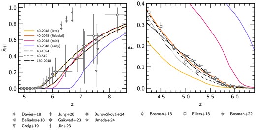
Left: evolution of the volume-averaged neutral fraction |$\bar{x}_{\rm H\,I}$| in the 40–2048 (coloured solid), 40–1024 (dot–dashed), 40–512 (dotted), and 160–2048 (long-dashed) runs. For the 40–2048 run, we show four different reionization models: late (gold), fiducial (orange), mid (dark pink), and early (purple) – see Table 1 for details. Also shown are observational constraints on |$\bar{x}_{\rm H\,I}$| derived from the effective optical depth of the Ly |$\alpha$| forest (Gaikwad et al. 2023); quasar damping wings (Bañados et al. 2018; Davies et al. 2018; Greig et al. 2019; Ďurovčíková et al. 2024, shown for the aton model constraints); the Ly |$\alpha$| emitter equivalent width distribution (Jung et al. 2020); Ly |$\alpha$| and Ly |$\beta$| dark pixel fractions (Jin et al. 2023); and galaxy damping wings (Umeda et al. 2024). Right: the mean transmission in the Ly |$\alpha$| forest over 50 |$h^{-1}\, {\rm cMpc}$| skewers, with constraints from Bosman et al. (2018), Eilers et al. (2018), and Bosman et al. (2022). The fiducial 40–2048 model is calibrated to reproduce the Bosman et al. (2018) and Eilers et al. (2018) results, while the 160–2048 model is calibrated to reproduce the Bosman et al. (2022) results.
The Sherwood–Relics project is primarily concerned with modelling the high-redshift IGM, and so does not include detailed subgrid physics models for galaxy formation. Instead, a computationally efficient density removal scheme – the ‘quick Ly |$\alpha$|’ approach – is employed, where gas particles with overdensity |$\rho _{\rm g}/\bar{\rho }_{\rm g} = \Delta > 1000$| and temperature |$T< 10^5~{\rm K}$| are converted to collisionless star particles (Viel, Haehnelt & Springel 2004). The simulations do not include any prescription for stellar feedback. Halo finding is performed using the inbuilt friends-of-friends (FoF) halo finder with a linking length of 0.2 times the mean interparticle spacing (Springel 2005). When we discuss ‘halo masses’, we are referring to the total FoF group mass |$M_{\rm h} = M_{\rm h,d}+ M_{\rm h,g} + M_{\rm h, \star }$|, where |$M_{\rm h,d}$|, |$M_{\rm h,g}$|, and |$M_{\rm h, \star }$| are the dark matter, gas, and stellar components of the FoF group, respectively.
Sightlines are drawn through the simulation volume to extract the relevant quantities for computing mock Ly |$\alpha$| absorption spectra. We draw 5000 such sightlines, with a spatial resolution of |$28.8~{\rm ckpc}$| (|$115.2~{\rm ckpc}$|) for the |$40~h^{-1}\, {\rm Mpc}$| (|$160~h^{-1}\, {\rm Mpc}$|) box. These sightlines are then post-processed to compute the Ly |$\alpha$| optical depths, using the approximation to the Voigt line profile due to Tepper-García (2006) and including, unless otherwise stated, the effects of peculiar velocities. Note that we do not attempt to model observational effects (e.g. noise, spectral resolution, total spectrum length) in these mock spectra, instead deferring a study of these effects for future work (see also Garaldi & Bellscheidt 2024a, for a recent study exploring the impact of these effects).
2.2 Real-space Ly α transmission
Before proceeding further, to develop some intuition about the nature of the galaxy–Ly |$\alpha$| transmission correlation, following Kulkarni et al. (2015) we consider the real-space Ly |$\alpha$| transmission. We will return to examining the full line-of-sight calculation of Ly |$\alpha$| optical depths, including redshift space distortions, in Section 3. The real-space Ly |$\alpha$| transmission is defined as
where |$\lambda _\alpha =1216~\rm{\mathring{\rm A}}$| is the rest-frame Ly |$\alpha$| wavelength, |$\Lambda _\alpha =6.265\times 10^{-8}{~\rm s^{-1}}$|, |$H(z)$| is the Hubble parameter, |${\bar{n}}_{\rm H}$| is the mean number density of hydrogen, |$\Delta$| is the overdensity, and |$x_{\rm H\,I}$| is the neutral hydrogen fraction, which depends on both the photoionization rate, |$\Gamma _{\rm H\,I}$|, and the gas temperature, T. Note that equation (1) is equal to |$\operatorname{exp}(-\tau _{\rm GP})$|, where |$\tau _{\rm GP}$| is the Gunn–Peterson optical depth (Gunn & Peterson 1965) and, unlike the calculations performed in the rest of this work, equation (1) ignores the effect of peculiar velocities and thermal line broadening on the Ly |$\alpha$| optical depth, and assumes that the line profile is a Dirac delta function at |$\lambda =\lambda _{\alpha }$|.
We calculate |$F_{\rm real}$| by first depositing the particles in the simulation on to a uniform grid using the SPH kernel; the Ly |$\alpha$| transmission can then be computed for each pixel independently. Next, we must select the haloes that host galaxies in the simulation. Measurements of the galaxy–Ly |$\alpha$| transmission correlation often use different methods for the detection of galaxies, such as C iv absorption or [O iii] emission. Given these differing detection methods, it is not immediately clear how to relate the sources of absorption in the observations to the structures in our simulations. Meyer et al. (2019) used abundance matching arguments to relate the incidence of C iv absorbers per absorption distance |${\rm d}\mathcal {N}/{\rm d}X$| to the halo mass function and thus obtain an approximate lower mass limit on the haloes hosting these absorbers, finding |$M_{\rm h}\gtrsim 10^{9.8}~h^{-1}\, {\rm M}_\odot$|. Their measurement of the C iv absorber bias is very uncertain, however, and is consistent with host halo masses as large as |$M_{\rm h}\sim 10^{12.4}~h^{-1}\, {\rm M}_\odot$|. Pizzati et al. (2024) use the FLAMINGO simulations (Schaye et al. 2023) to reproduce observations of the cross-correlation of high-z galaxies (selected through [O iii] emission), finding that the characteristic host halo mass of an [O iii] emitter is |$\approx 10^{10.7}~h^{-1}\, {\rm M}_\odot$|. However, Garaldi et al. (2022) and Garaldi & Bellscheidt (2024a) found that the exact choice of selection criteria (e.g. C iv column density or halo mass) makes only a small impact on the galaxy–Ly |$\alpha$| transmission correlation. Motivated by these arguments, here and throughout the rest of this work we therefore compute the galaxy–Ly |$\alpha$| transmission correlation for haloes with |$M_{\rm h} \ge 10^{10}~h^{-1}\, {\rm M}_\odot$|, unless otherwise specified. Finally, we extract a slice of depth |$115.2~{\rm ckpc}$| for each halo with |$M_{\rm h}\ge 10^{10}~h^{-1}\, {\rm M}_\odot$| in the fiducial 40–2048 simulation, by recentring the grids on the centre of mass of every halo. We stack slices to compute the average value of |$F_{\rm real}$| in each pixel, before normalizing by the global volume-averaged transmission |$\bar{F}_{\rm real}$|.
Fig. 2 displays the normalized stacked transmission |$F_{\rm real}/\bar{F}_{\rm real}$| at |$z=7,6,5.4,~{\rm and}~4.2$|. We show the result for the fiducial 40–2048 simulation, but note that the general features are the same for the other reionization models (aside from differences in timing due to the different reionization histories). At all redshifts shown in Fig. 2, there is a central region (|$\sim$| few cMpc in extent) where |$\log _{10}(F_{\rm real}/{\bar{F}}_{\rm real}) \ll 0$| (i.e. the Ly |$\alpha$| transmission is lower than average). At |$z=7$|, this region of low transmission is followed by an annulus of excess transmission (i.e. |$\log _{10}(F_{\rm real}/{\bar{F}}_{\rm real}) > 0$|), extending out to a radius of |$\sim 10{~\rm cMpc}$|. Beyond this region, the transmission again drops below the average. The picture is similar for |$z=6$| and |$z=5.4$|, but the central reduction in transmission is stronger, and the excess transmission begins at a larger distance from the halo, extends further, and is weaker. By |$z=4.2$| the central region of low transmission is the only feature that is still visible in the map.
![Logarithm of the normalized real-space Ly $\alpha$ transmission in stacked slices, each centred on a halo with mass $M_{\rm h} \ge 10^{10}~h^{-1}\, {\rm M}_\odot$ for the fiducial 40–2048 model. Each slice has width $40~h^{-1}\, {\rm cMpc}$ and depth $115.2~{\rm ckpc}$. We show the stacked transmission fluctuation at fixed redshifts of (from left to right) $z=7.0$, 6.0, 5.4, and 4.2, where each stack is produced from 2431, 4540, 6191, and 10 706 slices, respectively. To highlight the structure of the transmission correlation, we clip the dynamic range of the colour scale to be from $\bar{F}_{\rm real}/4$ to $4 \bar{F}_{\rm real}$, as indicated by the arrows on the colour bar. Also shown for comparison (see Section 3.3 for a discussion) is the distance at which the halo–Ly $\alpha$ transmission correlation (calculated without including peculiar velocities) is largest [‘$r(\delta _{F,{\rm max}})$’, black solid circle], and the mean free path of Lyman limit photons around haloes from Feron et al. (2024) (‘$\Lambda _{\rm mfp}$’, black dashed circle).](https://oup.silverchair-cdn.com/oup/backfile/Content_public/Journal/mnras/539/3/10.1093_mnras_staf648/2/m_staf648fig2.jpeg?Expires=1750220199&Signature=5EA37gLxqtym5e-lGDY8SboYCsh4UnBK8HpEsTqsfOa4wewAoNDTCRiHF-17pkSczgtIqzZOoTW7FOMRx7lNXOjWM5JZNJtNoNTmR8roiw-AKW2emcUgHcg9CAUkPu2diOM2G4AEQDB6LGjskXM5Wuisb7HdgPqmnSPgraa17qstccWgOUphWeegUiHAc8x9kpdp6mHMjWfGG6rwFZRNN~uIXplGzaq0o-qEcGXcT~7Ejp2334ArGDmZPx93g80q9WD8jjj8plvfjEt8F5doOBWmaV89GA-BXS3zWTbOjCTyc~x0aJtYncwp5gomSv7DIV2nTfxsKtPLUSFHpchxYg__&Key-Pair-Id=APKAIE5G5CRDK6RD3PGA)
Logarithm of the normalized real-space Ly |$\alpha$| transmission in stacked slices, each centred on a halo with mass |$M_{\rm h} \ge 10^{10}~h^{-1}\, {\rm M}_\odot$| for the fiducial 40–2048 model. Each slice has width |$40~h^{-1}\, {\rm cMpc}$| and depth |$115.2~{\rm ckpc}$|. We show the stacked transmission fluctuation at fixed redshifts of (from left to right) |$z=7.0$|, 6.0, 5.4, and 4.2, where each stack is produced from 2431, 4540, 6191, and 10 706 slices, respectively. To highlight the structure of the transmission correlation, we clip the dynamic range of the colour scale to be from |$\bar{F}_{\rm real}/4$| to |$4 \bar{F}_{\rm real}$|, as indicated by the arrows on the colour bar. Also shown for comparison (see Section 3.3 for a discussion) is the distance at which the halo–Ly |$\alpha$| transmission correlation (calculated without including peculiar velocities) is largest [‘|$r(\delta _{F,{\rm max}})$|’, black solid circle], and the mean free path of Lyman limit photons around haloes from Feron et al. (2024) (‘|$\Lambda _{\rm mfp}$|’, black dashed circle).
The behaviour of the transmission in Fig. 2 may be understood by examining Fig. 3, where we show averages of the key quantities used in equation (1), namely gas overdensity |$\Delta$|, photoionization rate |$\Gamma _{\rm H\,I}$|, neutral hydrogen fraction |$x_{\rm H\,I}$|, and gas temperature T.2 The stacks in Fig. 3 are calculated in the same fashion as in Fig. 2. At all redshifts, |$\Delta$| is centrally concentrated with a value at |$r\gtrsim 20~{\rm cMpc}$| that gradually becomes smaller with time as structure formation progresses. At |$z=7$|, the local radiation field around the haloes is clearly visible in the excess |$\Gamma _{\rm H\,I}$| at |$r\lesssim 15~{\rm cMpc}$|. This drives a corresponding decrease in |$x_{\rm H\,I}$| and excess in T due to photoionization and photoheating, respectively (i.e. from the ionized bubbles around the sources). This is also demonstrated by the dashed circles in and Figs 2 and 3 which show the Lyman-limit mean free path around haloes, |$\Lambda _{\rm mfp}$|, from Feron et al. (2024).3 This implies the local radiation field from ionizing sources plays an important role in setting the galaxy–Ly |$\alpha$| transmission correlation. We return to discuss the solid circles in Figs 2 and 3 in Section 3.3.
![Stacked slices of the key quantities that set the real-space Ly $\alpha$ transmission displayed in Fig. 2 (the slices used to produce the stacks are the same as those used to make Fig. 2). From left to right, the columns show the fluctuations in gas density $\log _{10}\Delta =\log _{10}(\rho _{\rm g}/\bar{\rho }_{\rm g})$; hydrogen photoionization rate $\log _{10}(\Gamma _{\rm H\,I}/\bar{\Gamma }_{\rm H\,I})$; neutral hydrogen fraction $\log _{10}(x_{\rm H\,I}/\bar{x}_{\rm H\,I})$; and gas temperature $\log _{10}(T/\bar{T})$. In each case, barred quantities indicate the global volume average of a quantity. From top to bottom, the rows display the stacks for $z=7,6,5.4$, and 4.2. Note that in each case we clip the dynamic range of the colour map, in order to centre the mean and highlight structure (the clipped end of the colour bar is triangular). As in Fig. 2, we also show the distance at which the halo–Ly $\alpha$ transmission correlation is largest [‘$r(\delta _{F,{\rm max}})$’, solid circle], and the mean free path of Lyman limit photons around haloes from Feron et al. (2024) (dashed circle).](https://oup.silverchair-cdn.com/oup/backfile/Content_public/Journal/mnras/539/3/10.1093_mnras_staf648/2/m_staf648fig3.jpeg?Expires=1750220199&Signature=IVyxnc2f9fU5VriQVd21gzmrduk~EFN0dhQUYwKOzKCb6f0bTUT7IXc7o4iMOET2-tZfy8g0HXbsR5QbYG0JkwioJ8nBOVpF-NL~f5K-~6KUmPdPn2-cwv2ZPcd6WA~GWE92H3mWRipE4VrJnPihiqJkma77Cz9KgjhdqYSPi8bcN~Vzkncg72FQ3RnYIJkKqdwKBUIqOxuxMNQkhBJ6FvD9FxiC0L05ztlSyv5LULgp~oXbuWIHQoe37v9QDsMAzqp8l8aAknldul-jg7U6xzi1s7bEAY7jOzi4apQ5M0yE0SRcitfcfplU~-5tbTIWWQD3mhrNB04m8nkvcK4MBA__&Key-Pair-Id=APKAIE5G5CRDK6RD3PGA)
Stacked slices of the key quantities that set the real-space Ly |$\alpha$| transmission displayed in Fig. 2 (the slices used to produce the stacks are the same as those used to make Fig. 2). From left to right, the columns show the fluctuations in gas density |$\log _{10}\Delta =\log _{10}(\rho _{\rm g}/\bar{\rho }_{\rm g})$|; hydrogen photoionization rate |$\log _{10}(\Gamma _{\rm H\,I}/\bar{\Gamma }_{\rm H\,I})$|; neutral hydrogen fraction |$\log _{10}(x_{\rm H\,I}/\bar{x}_{\rm H\,I})$|; and gas temperature |$\log _{10}(T/\bar{T})$|. In each case, barred quantities indicate the global volume average of a quantity. From top to bottom, the rows display the stacks for |$z=7,6,5.4$|, and 4.2. Note that in each case we clip the dynamic range of the colour map, in order to centre the mean and highlight structure (the clipped end of the colour bar is triangular). As in Fig. 2, we also show the distance at which the halo–Ly |$\alpha$| transmission correlation is largest [‘|$r(\delta _{F,{\rm max}})$|’, solid circle], and the mean free path of Lyman limit photons around haloes from Feron et al. (2024) (dashed circle).
Toward lower redshift the fluctuations in |$\Gamma _{\rm H\,I}$| fade away as the intensity of the UV background (UVB) increases, and by |$z=5.4$| only the very central excess is visible. The effect of the diminishing UVB fluctuations are again mirrored in the behaviour of the neutral hydrogen fraction (and hence also |$F_{\rm real})$|. Lastly, at |$z=4.2$| (after the end of reionization) all the gas in the IGM is highly ionized and the central region in the stacked slice is more neutral than average due to the larger gas density (i.e. |$x_{\rm H\,I} \propto \Delta$| for gas in ionization equilibrium).
The behaviour of the temperature fluctuations, displayed in the right column of Fig. 3, is slightly different. The central region at all redshifts contains hot gas associated with shocks from structure formation. At |$z=7$|, the region around the stacked haloes (|$r\lesssim 15~{\rm cMpc}$|) is dominated by recently photoheated gas, which produces an excess in T relative to the average. By |$z=6$|, the excess in temperature is still present, but at larger distances (|$10\lesssim r/{\rm cMpc}\lesssim 30$|); regions further away from the sources have been more recently photoheated and have had less time to cool. Gas in the low-density IGM cools adiabatically via the expansion of the Universe and also through inverse Compton scattering off cosmic microwave background photons (an important process at these redshifts, see e.g. Puchwein et al. 2019), so the gas closer to the sources (|$1\lesssim r/{\rm cMpc}\lesssim 10$|) is instead now cooler than average. At |$z=5.4$| the picture is similar to |$z=6$|, but the excess in temperature occurs still further away from sources (|$r \gtrsim 15~{\rm cMpc}$|). By |$z=4.2$| the coherent radial fluctuations in temperature have largely faded, and the temperature more closely correlates with the density field (i.e. the IGM is relaxing toward a power-law temperature–density relation, |$T=T_{0}\Delta ^{\gamma -1}$|). The fact that–due to the long cooling time-scale for the low density IGM–relic fluctuations in temperature persist longer than the fluctuations in photoionization rate will have consequences for the post-reionization galaxy–Ly |$\alpha$| transmission correlation (see also D’Aloisio et al. 2018; Keating, Puchwein & Haehnelt 2018; Molaro et al. 2023, for related work). We will discuss this further in Section 4.3.
3 THE GALAXY–LY |${\alpha} $| TRANSMISSION CORRELATION IN SHERWOOD–RELICS
3.1 Computing the galaxy–Ly |${\alpha} $| transmission correlation
We now turn to examine the galaxy–Ly |$\alpha$| transmission correlation using our mock Ly |$\alpha$| forest spectra that include redshift space effects. We do this by selecting each halo that satisfies a given mass constraint (usually |$M_{\rm h}\ge 10^{10}~h^{-1}\, {\rm M}_\odot$|) and then calculating the distance to each pixel in our Ly |$\alpha$| forest sightlines. We then use bins of width |$\Delta r=147~{\rm ckpc}$| and average the transmission over many sightlines to obtain |$\langle F(r) \rangle$|. The galaxy–Ly |$\alpha$| transmission correlation is then
where |$\bar{F}$| is the global volume-averaged Ly |$\alpha$| transmission at that redshift, computed from the simulated spectra. Throughout the remainder of this work we therefore also refer to the galaxy–Ly |$\alpha$| transmission correlation as |$\delta _F$|. For the sake of clarity, we note that |$\delta _F< 0$| corresponds to less transmission than the average, and |$\delta _F>0$| corresponds to more.
3.2 Comparison with observational data
We begin with a comparison to observational data at |$z< 4$|, well after reionization has completed. In Fig. 4, we compare these data to |$\delta _F$| as a function of distance r from haloes with |$M_{\rm h}\ge 10^{10}~h^{-1}\, {\rm M}_\odot$| in the 40–2048 and 160–2048 models at |$z \le 5.4$|. This redshift corresponds roughly to the endpoint of reionization in the simulations (i.e. where the volume-averaged neutral fraction |$\bar{x}_{\rm H\,I} \le 10^{-3}$|, see Table 1). In both the 40–2048 and 160–2048 runs, |$\delta _F < 0$| close to the haloes, where |$\delta _F$| decreases rapidly with decreasing distance. Furthermore, at fixed r, |$\delta _F$| increases with decreasing redshift. For the 40–2048 run, |$\delta _F$| drops below |$-0.1$| at |$r\lesssim 5$|–|$10{~\rm cMpc}$|, depending on redshift, while for 160–2048 the same decrease in |$\delta _F$| occurs at |$r\lesssim 10$|–|$20{~\rm cMpc}$|. This decrement in |$\delta _F$| over larger distances in the 160–2048 run is due to the more massive haloes present in the larger volume, which sit in larger associated overdensities (see Fig. A1). For |$r>20{~\rm cMpc}$| (|$50~{\rm cMpc}$|) in the 40–2048 (160-2048) run, the transmission approaches the mean value (i.e. |$\delta _F\rightarrow 0$|).
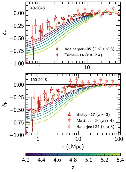
The low-redshift (|$z\le 5.4$|) galaxy–Ly |$\alpha$| transmission correlation (|$\delta _F$|, see equation 2) as a function of distance r from haloes with mass |$M_{\rm h} \ge 10^{10}~h^{-1}\, {\rm M}_\odot$| in the fiducial 40–2048 (solid, top panel) and 160–2048 (dashed, bottom panel) simulations. Both models are shown every |$\Delta z= 0.2$| between |$z=4.2$| and |$z=5.4$|. We also show constraints from |$2 \le z \le 4$| due to Adelberger et al. (2005), Turner et al. (2014), Bielby et al. (2017), Banerjee et al. (2024), and Matthee et al. (2024). Note the different ranges in r between the top and bottom panels. Redshift differences between the data and simulations mean we do not expect quantitative agreement.
The shape of |$\delta _F$| predicted by the models is in qualitative agreement with observations, and where the redshift of the data points and simulations are similar (|$z\sim 4$|) the agreement is reasonable. However, we do not expect perfect quantitative agreement between our models and observations, given that the observations are at (often much) lower redshift (the closest observations to our lowest redshift snapshot at |$z=4.2$| are the Matthee et al. 2024 results, at |$z\approx 4$|). In addition, we note again that the lack of a detailed subgrid model for galaxy formation and feedback (which may be important for matching observations of |$\delta _F \ll 0$| close to galaxies, see Meiksin et al. 2017; Sorini et al. 2020) in Sherwood–Relics means that we do not expect good agreement close to (|$r \lesssim 1{~\rm cMpc}$|) haloes.
In Figs 5–8, we now focus on the data at redshifts approaching the reionization era. We show |$\delta _F$| for |$z > 5.4$| compared to observational constraints from Meyer et al. (2019, 2020), Kashino et al. (2023), and Kakiichi et al. (2025), respectively. Beginning with the general features of |$\delta _F$| in our models at high z, we observe a similar rapid decrease in |$\delta _F$| close to haloes as observed at lower z, but now |$\delta _F > 0$| further away from haloes (|$r\gtrsim {\rm few ~cMpc}$|). For both the 40–2048 and 160–2048 models, the amplitude of this excess is larger at higher z, when there is very little transmission in the IGM (i.e. the excess is not driven by a very large |$\langle F(r)\rangle$|, but rather the contrast with small |$\bar{F}$|). As redshift decreases, the peak of the excess shifts to larger distances, from |$r\approx 6{~\rm cMpc}$| (|$r\approx 12{~\rm cMpc}$|) at |$z=7$| for 40–2048 (160-2048) to |$r \sim 20 {~\rm cMpc}$| at |$z=6$| for both models, although around |$z=6$| the ‘peak’ becomes very broad. For |$r \gtrsim 20~{\rm cMpc}$| (|$r\gtrsim 60~{\rm cMpc}$|) at |$z\ge 6$|, |$\delta _F$| becomes negative again in the 40–2048 (160-2048) model, due to gas in the IGM that has not yet been highly ionized.
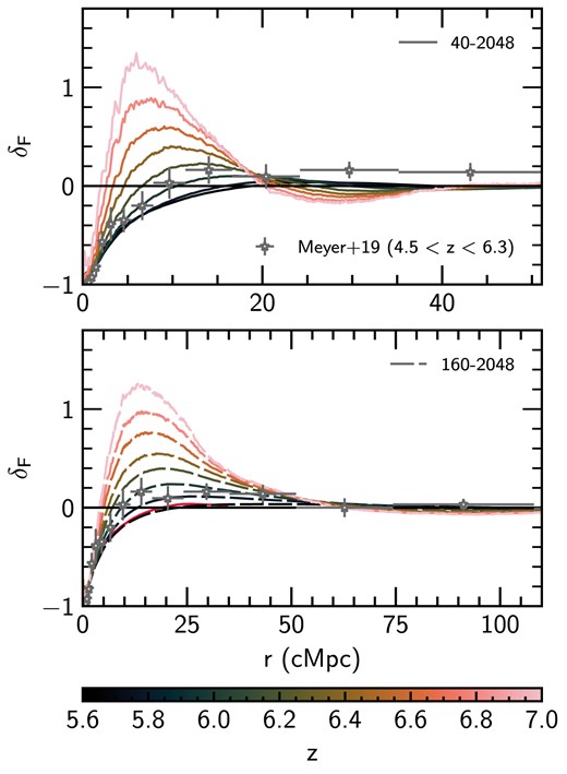
The high-redshift (|$z > 5.4$|) galaxy–Ly |$\alpha$| transmission correlation (|$\delta _F$|, see equation 2) as a function of distance r from haloes with mass |$M_{\rm h} \ge 10^{10}~h^{-1}\, {\rm M}_\odot$| in the fiducial 40–2048 (solid, top and bottom panels) and 160–2048 (dashed, bottom panel) simulations. We show |$\delta _F$| at |$z=6$| from the 40–2048 model in the bottom panel (solid, red) to aid comparison. Both models are shown every |$\Delta z= 0.2$| between |$z=5.6$| and |$z=7.0$|. Also shown are observational constraints due to Meyer et al. (2019), calculated using C iv absorbers over the redshift range |$4.5 < z_{\rm C\, {\small IV}} < 6.3$| (with mean redshift |$\langle z_{\rm C\, {\small IV}}\rangle = 5.18$|) as proxies for galaxies (see Section 2.2 for a discussion on the selection criteria for haloes). Note the different ranges in r between the top and bottom panels.

![As in Fig. 5, but shown over a smaller range in r and with constraints from Kashino et al. (2023), where [O iii] emitters were used in the calculation of $\delta _F$. In the interests of readability, the higher (lower) redshift (Kashino et al. 2023) points have been offset by 0.2 ($-0.2$) cMpc and we do not show the full extent of the higher redshift (Kashino et al. 2023) data, which extends up to $\delta _F \approx 3$ at $r\approx 5 {~\rm cMpc}$. Note that both the top and bottom panels now share the same range in r.](https://oup.silverchair-cdn.com/oup/backfile/Content_public/Journal/mnras/539/3/10.1093_mnras_staf648/2/m_staf648fig7.jpeg?Expires=1750220199&Signature=j8AcsB4IYoxr3IyKzv2L7SnKeHcfQ1zepnmJ~yVACLX4IMRhGrZuW-tGJUbfaMlb-euCr1ZB2q5io3v8R9GWw1m5smcNwLrG6XJR6D27AFZotzaE2p0zCxe1DLbvtagWrzHrXaWtOPELm17UtlRjHGkhKxMUIlLBxaCGL9BtKLswPyv46iLQEQ3rcC-jUCIebLcn27CP71QLI1tpyquxBFZa-jmi8B6q8BxYdCmmWHnL7X1aoNcuLedBFFia29aFdtkKFmaMOU1v61LKbrkV~ud8oJpnQQFihbcTCkMGN~~Px58HOT-p072yLnP64elEccPY7CHnx6Er0LtAGxcfHA__&Key-Pair-Id=APKAIE5G5CRDK6RD3PGA)
As in Fig. 5, but shown over a smaller range in r and with constraints from Kashino et al. (2023), where [O iii] emitters were used in the calculation of |$\delta _F$|. In the interests of readability, the higher (lower) redshift (Kashino et al. 2023) points have been offset by 0.2 (|$-0.2$|) cMpc and we do not show the full extent of the higher redshift (Kashino et al. 2023) data, which extends up to |$\delta _F \approx 3$| at |$r\approx 5 {~\rm cMpc}$|. Note that both the top and bottom panels now share the same range in r.
![As in Fig. 5, but with constraints from Kakiichi et al. (2025), where $\delta _F$ is computed for [O iii] emitters over the redshift range $5.4 < z_{\rm [O\, {\small III}]} < 6.5$ (with mean redshift $\langle z_{\rm [O\, {\small III}]}\rangle = 5.86$).](https://oup.silverchair-cdn.com/oup/backfile/Content_public/Journal/mnras/539/3/10.1093_mnras_staf648/2/m_staf648fig8.jpeg?Expires=1750220199&Signature=z5~nA-lis64tSOncYG1cx70z34oLC-Fzs28H1zu72Z0z2Yt9Zrx5bphAymFgOjiIuuQ~T8m75C6Y~9ck7WwZg5CfNi~tWFGH0UhVYoESbPWR3wvmgFCgNISRHHl2xLP5bZvv51arn2kLv-Dh1l1xIscuuDqJR8IIEcXUDx5uNNbNeoEEiv6O7mlfXXtOXV7J0Z-eKfsrfe-GXZPdrfiePbVEetA9cljmgAlYQW2gFe7A8MK-fKFKDL7xklyWnmBQluU7f63SoFoveBgic9qYEUlNGM51KG9jyqfPtA~TRR4lBm54GWlRK58gE1H9bl0IkEjsGkeWC9-1OCTck2pxJg__&Key-Pair-Id=APKAIE5G5CRDK6RD3PGA)
Turning now to comparing the high-z |$\delta _F$| in our models to observational data, we begin with Fig. 5 and the Meyer et al. (2019) constraints. Meyer et al. (2019) use the positions of C iv absorbers over the redshift range |$4.5 < z_{\rm C\, {\small IV}} < 6.3$| (with mean redshift |$\langle z_{\rm C\, {\small IV}} \rangle = 5.18$|) as proxies for galaxies when computing |$\delta _F$|. As discussed in Section 2.2, they argue that these absorbers approximately correspond to halo masses |$M_{\rm h} \gtrsim 10^{9.8}~h^{-1}\, {\rm M}_\odot$|, although note the observed C iv bias they report is uncertain and is consistent with host halo masses as large as |$M_{\rm h}=10^{12.4}~h^{-1}\, {\rm M}_\odot$|. For |$r \lesssim 20~{\rm cMpc}$|, we find excellent agreement (|$< 1\sigma$|) between the Meyer et al. (2019) results and our fiducial 40–2048 model, but at |$z=6$| as opposed to |$\langle z_{\rm C\, {\small IV}} \rangle = 5.18$|. Interestingly, a qualitatively similar result was also independently noted by Garaldi et al. (2022) using the THESAN simulations, where these authors found simulation outputs at |$z\sim 6.2$| were in better agreement with the Meyer et al. (2019) data. In addition to the timing discrepancy, for |$r \gtrsim 20~{\rm cMpc}$| we are unable to reproduce the observed |$\delta _F>0$| at any of the redshifts shown. For the 160–2048 model, we also find excellent agreement at |$z=6$| (mostly |$< 1\sigma$|) over the entire range shown (|$110~{\rm cMpc}$|).4 Again, this redshift, at which the 160–2048 model best agrees with the data, is higher than the average redshift of C iv absorbers in the Meyer et al. (2019) data set. This is perhaps surprising, given that our simulations are calibrated to reproduce observations of the mean transmission in the Ly |$\alpha$| forest at |$z\lesssim 6$|, but it is equivalent to requiring |$\bar{x}_{\rm H\,I}\sim 0.1$| at |$z=5.2$|. For comparison, the distribution of Ly |$\alpha$| effective optical depths at |$z \le 5.2$| are consistent with a fully reionized IGM and a homogeneous UV background, suggesting there is little scope for delaying the end of reionization below this redshift (Bosman et al. 2022).
We move now to Fig. 6 and the follow-up work of Meyer et al. (2020), where the cross-correlation is computed for LBGs and Ly |$\alpha$| emitters (LAEs) at |$z\sim 6$| as opposed to C iv absorbers at slightly lower redshift. In contrast to the Meyer et al. (2019) result, we find poor agreement with the Meyer et al. (2020) constraints, except for the negative |$\delta _F$| at small (|$r\lesssim 5~{\rm cMpc}$|) scales. Indeed, Meyer et al. (2020) note that their measurement is impacted by the small sample size and noise, and argue that the two-point cross-correlation function between transmission spikes (high signal-to-noise pixels with |$F>0.02$|) and galaxy positions should provide a more robust measurement. We briefly discuss this statistic in Appendix B, but focus on the more widely used |$\delta _F$| throughout the main portion of this work.
Next, we turn to Fig. 7 and the comparison with the Kashino et al. (2023) constraints from a single QSO field from the EIGER survey. Kashino et al. (2023) use [O iii]-emitting galaxies when calculating |$\delta _F$| and, while we do not directly model [O iii] emission, it has been shown that these [O iii] emitters tend to reside in haloes with |$M_{\rm h}\approx 10^{10.7}~h^{-1}\, {\rm M}_\odot$| (Pizzati et al. 2024, see also discussion in Section 2.2). For |$z\sim 7$|, we reproduce some general features of the Kashino et al. (2023) measurement for |$r\lesssim 10 {~\rm cMpc}$|, namely |$\delta _F< 0$| at small distances (|$r\lesssim 4{~\rm cMpc}$|) and a strongly peaked excess in |$\delta _F$| at slightly larger distances (|$r \approx 6{~\rm cMpc}$|), but are unable to match the extreme value of |$\delta _F\approx 3$| at |$r\approx 5\rm \, cMpc$| (not shown in Fig. 7, see figure caption) or the behaviour of |$\delta _F$| for |$r\gtrsim 10{~\rm cMpc}$|. Our analysis is consistent with the interpretation of Garaldi & Bellscheidt (2024a), who suggest that the Kashino et al. (2023) result is likely dominated by stochasticity, given that it focuses on a single QSO sightline. Future results from all six QSO fields in the EIGER survey could provide interesting new insights into the nature of the galaxy–Ly |$\alpha$| transmission correlation at high z. In the context of modelling, varying the source model in our simulations could also prove instructive, particularly for small r.
While this work was being completed, new results on the [O iii] emitter–Ly |$\alpha$| transmission correlation were released by the JWST ASPIRE survey (Kakiichi et al. 2025) using five QSO fields. In Fig. 8, we show the Kakiichi et al. (2025) results compared to our fiducial 40–2048 and 160–2048 models. For the 40–2048 model at |$z=5.8$| – approximately the mean redshift of the [O iii] emitters used in Kakiichi et al. (2025) – the simulation is within |$1\sigma$| of the Kakiichi et al. (2025) results for |$r \lesssim 20~{\rm cMpc}$|. However, the 40–2048 model does not match the shape of |$\delta _F$| (which peaks around |$r\approx 30~{\rm cMpc}$|) at larger |$r\gtrsim 20~{\rm cMpc}$|. For the 160–2048 model at |$z=5.8$|, the agreement is much better and the simulation is within |$1.5 \sigma$| of the Kakiichi et al. (2025) results over the entire range of r shown, although the peak in |$\delta _F$| occurs at a smaller |$r\approx 20~{\rm cMpc}$| in the 160–2048 model than in the observational data. As we will discuss in Section 4.1, selecting a larger minimum halo mass for the haloes used in the calculation of |$\delta _F$| may improve the agreement further (cf. Fig. 9). A box size larger than |$160~h^{-1}\rm \, cMpc$| may also be required to fully capture the largest ionized bubbles and the ionizing sources clustering around massive haloes.
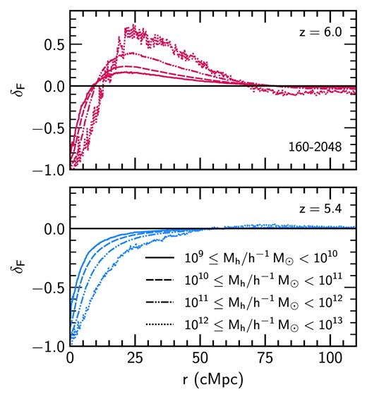
Impact of halo mass used in the calculation of the galaxy-Ly |$\alpha$| transmission fluctuation correlation in the 160–2048 run at |$z=6.0$| (top panel, pink) and |$z=5.4$| (bottom panel, blue). We show the correlation between our simulated spectra and haloes in bins spanning four decades in mass: |$10^{9}\le M_{\rm h}/h^{-1}\, {\rm M}_\odot < 10^{10}$| (solid), |$10^{10}\le M_{\rm h}/h^{-1}\, {\rm M}_\odot < 10^{11}$| (dashed), |$10^{11}\le M_{\rm h}/h^{-1}\, {\rm M}_\odot < 10^{12}$| (dash–dot–dotted), and |$10^{12}\le M_{\rm h}/h^{-1}\, {\rm M}_\odot < 10^{13}$| (dotted).
3.3 The galaxy–Ly |${\alpha} $| transmission correlation and the local mean free path around haloes
Finally, we explore the connection between the location of the peak of |$\delta _F$| in Figs 5–8 and the local mean free path of Lyman-limit photons around galaxies, as highlighted recently by Garaldi & Bellscheidt (2024a). In this case, we calculate |$\delta _F$| without including the effect of peculiar velocities to enable a fair comparison with the real-space Ly |$\alpha$| transmission defined in equation (1). We compute the distance at which |$\delta _F$| is largest, |$r(\delta _{F,{\rm max}})$|, by first smoothing |$\delta _F$| with a moving window of eight times the bin width (|$\Delta r=1180~{\rm ckpc}$|) to reduce noise (for comparison, Garaldi & Bellscheidt 2024a use a window of |$2950~{\rm ckpc}$|).
We show |$r(\delta _{F,{\rm max}})$| as a solid circle in Figs 2 and 3. At all redshifts, |$r(\delta _{F,{\rm max}})$| occurs well away from the high-density peak associated with the haloes. At |$z=7$| and |$z=6$|, |$r(\delta _{F,{\rm max}})$| sits inside the region where the radiation field is enhanced relative to the background, and the hydrogen is correspondingly more ionized. At |$z=5.4$| however, after the radiation field becomes close to homogeneous, the (very small) peak that remains for the excess transmission approximately coincides with the residual excess in the gas temperature. The behaviour of the halo mean free path, |$\Lambda _{\rm mfp}$|, measured from Sherwood–Relics by Feron et al. (2024)5 (dashed circles) is qualitatively similar to that of |$r(\delta _{F,{\rm max}})$|. There will be small differences due, in part, to the slightly different sample of haloes used to calculate |$\Lambda _{\rm mfp}$| in Feron et al. (2024) (see also Section 4.1). Nevertheless, as first noted recently by Garaldi & Bellscheidt (2024a), this suggests the typical scale for the excess transmission in the galaxy–Ly |$\alpha$| transmission correlation is related to the local mean free path for ionizing photons around galaxies. Prior to the end of reionization, this quantity will be larger than the mean free path in the average IGM, but following reionization it will be smaller [see e.g. fig. 8 in Feron et al. (2024) and the related discussion, as well as Fan et al. (2025)].
4 THE DETAILED PHYSICAL ORIGIN OF THE GALAXY–LY |${\alpha} $| CORRELATION
4.1 Degeneracy between halo mass and neutral fraction
We now turn to more closely examine the various factors that influence the galaxy–Ly |$\alpha$| correlation in our simulations. First, we examine the galaxy–Ly |$\alpha$| transmission correlation computed using only haloes in a given mass range in Fig. 9. We consider the results from the 160–2048 model at |$z=6$| and |$z=5.4$|, although note that the general trends are the similar in the 40–2048 box. Here we use the 160–2048 box instead of the fiducial, higher-resolution 40–2048 box because it contains haloes with larger masses, |$M_{\rm h} > 10^{12}~h^{-1}\, {\rm M}_\odot$| while also still resolving the minimum halo mass |$M_{\rm h} = 10^{9}~h^{-1}\, {\rm M}_\odot$| that hosts ionizing sources in our simulations (see e.g. Fig. A1). We compute |$\delta _F$| for haloes spanning four decades in mass, although note the lowest mass bin (|$10^{9}\le M_{\rm h}/h^{-1}\, {\rm M}_\odot < 10^{10}$|) is shown only for comparison here and is not used throughout the rest of this work. For mass bins with |$M_{\rm h}\ge 10^{10}~h^{-1}\, {\rm M}_\odot$| we use all haloes when calculating |$\delta _F$| and, for computational efficiency, we draw a representative sample of |$10^4$| haloes for those with |$10^{9}\le M_{\rm h}/h^{-1}\, {\rm M}_\odot < 10^{10}$|. At |$z=6$| (|$z=5.4$|) the largest halo has a mass of |$4.5\times 10^{12}~h^{-1}\, {\rm M}_\odot$| (|$6.9\times 10^{12}~h^{-1}\, {\rm M}_\odot$|).
In the lower panel of Fig. 9 at |$z=5.4$| (close to the end of reionization), for |$r\lesssim 50~{\rm cMpc}$| we find that the radial extent of the region with negative |$\delta _F$| becomes larger as the halo mass used to calculate |$\delta _F$| increases. This is because the lower-mass haloes are associated with smaller overdensities where the clustering and infall of neutral hydrogen is weaker. In photoionization equilibrium, |$\Delta \propto x_{\rm H\,I}$|, and in the absence of a strong proximity effect or feedback we therefore expect the gas approaching the lower-mass haloes to have smaller |$x_{\rm H\,I}$| (i.e. are more highly ionized) and larger transmission (i.e. a smaller region of negative |$\delta _F$|).
The results displayed in the upper panel of Fig. 9 at |$z=6$| are more complicated, however. Due to proximity to the ionizing sources, the gas within |$r\lesssim 5{~\rm cMpc}$| is reionized earlier than gas further away (see e.g. fig. 1 in Puchwein et al. 2023). Therefore, by |$z=6$|, this gas is already in photoionization equilibrium and the behaviour observed at |$z=5.4$| is replicated. However, further away from haloes (|$10 \lesssim r/{\rm cMpc}\lesssim 70$|), it is now the more massive haloes which have larger, positive |$\delta _F$| (i.e. excess transmission relative to the mean). This is because, in the Sherwood–Relics model, the ionizing emissivity of a source, |$\dot{N}_\gamma$|, is proportional to halo mass (Kulkarni et al. 2019); when the IGM is optically thin to ionizing photons the photoionization rate in the low-density IGM (i.e. far away from haloes where local density effects become unimportant) is always larger around more massive haloes due to source clustering. We therefore speculate that simulations which use a different source luminosity assignment, such as a ‘Democratic’ model where |$\dot{N}_\gamma$| is independent of |$M_{\rm h}$| (Cain et al. 2023; Asthana et al. 2024b), may change these results. Temperature fluctuations also play a role, as gas that is ionized (and therefore heated) earlier has more time to cool than gas which is ionized later. At a given density, colder gas is more neutral (since the recombination coefficient scales as |$\alpha \propto T^{-0.72}$| for gas |$T\sim 10^4~{\rm K}$|) and so the (relatively) cooler gas near to haloes will also exhibit reduced transmission compared to the hotter gas farther away.
In Fig. 10, we instead compare |$\delta _F$| for the three additional reionization models listed in Table 1 to the fiducial model (solid curves in each panel). The redshift evolution of the galaxy–Ly |$\alpha$| transmission correlation is different for each reionization model. Hence, rather than compare these models at fixed redshift, in Fig. 10 we instead compare the models to the fiducial model at approximately the same volume averaged neutral hydrogen fraction. We do this by finding the closest match in |$\bar{x}_{\rm H\,I}$| between the fiducial model and each reionization model. In Table 2, we list the redshifts and corresponding neutral hydrogen fractions for the matched outputs. For the different reionization models, we use snapshots at |$z=7,\, 6$| and 5.4, except for the early model where we only use snapshots at |$z=7$| and 6. This is because the fiducial model was not run to low enough redshift to match the neutral hydrogen fraction at |$z=5.4$| in the early model.
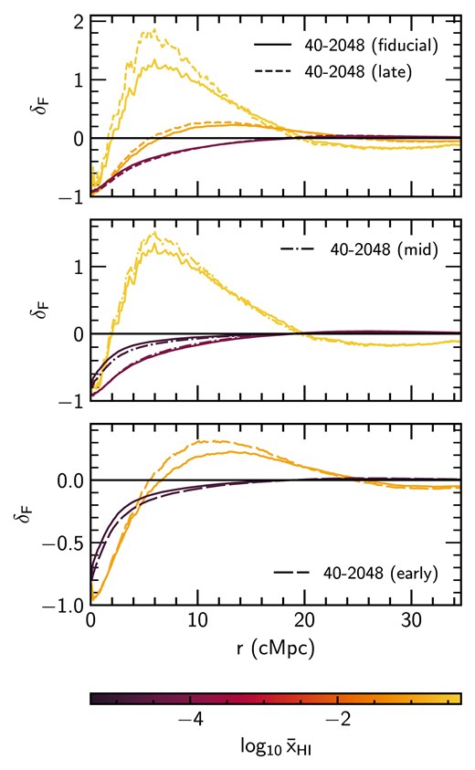
Comparison of different reionization histories to the fiducial 40–2048 run at approximately equal volume weighed IGM neutral hydrogen fractions, |$\bar{x}_{\rm H\,I}$|. Shown are the late (top panel, dashed), mid (middle panel dot–dashed) and early (bottom panel, long dashed) reionization models along with the fiducial model (solid, with the same curves are shown in all panels). The colour indicates |$\log _{10}\bar{x}_{\rm H\,I}$|. In each case, we select the closest match in |$\bar{x}_{\rm H\,I}$| between the fiducial model values and each of the three reionization models measured at |$z=7, 6$| and 5.4. We do not show |$\delta _F$| at |$z=5.4$| for the early model, as the fiduical model does not extend to low enough redshift to match the neutral hydrogen fraction. Note the neutral fraction decreases with decreasing redshift, so in each panel the curves with larger (smaller) |$\bar{x}_{\rm H\,I}$| correspond to higher (lower) redshift outputs for each model.
Redshifts and neutral fractions for the |$\delta _F$| shown in Fig. 10. Listed in the columns are: the model name and reionization redshift, |$z_{\rm r}$| (see also Table 1), the corresponding volume weighted neutral hydrogen fraction, |$\bar{x}_{\rm H\,I}$|, at redshift z in each of these models, and the redshift, |$z_{\rm match}$|, and volume weighted neutral hydrogen fraction, |$\bar{x}_{\rm H\,I,match}$|, in our fiducial reionization model (|$z_{\rm r}=5.7$|) that most closely matches |$\bar{x}_{\rm H\,I}$|. We do not include the early model at |$z=5.4$|, as the fiducial model does not extend to low enough redshift to provide a good match in |$\bar{x}_{\rm H\,I}$|.
| Reionization model | z | |$\bar{x}_{\rm H\,I}$| | |$z_{\rm match}$| | |$\bar{x}_{\rm HI,match}$| |
|---|---|---|---|---|
| Late (|$z_{\rm r}=5.3$|) | 7.0 | 0.47 | 7.0 | 0.41 |
| 6.0 | 0.14 | 6.2 | 0.12 | |
| 5.4 | |$10^{-2.48}$| | 5.6 | |$10^{-4.08}$| | |
| Mid (|$z_{\rm r} = 6.0$|) | 7.0 | 0.44 | 7.0 | 0.41 |
| 6.0 | |$10^{-2.62}$| | 5.6 | |$10^{-4.08}$| | |
| 5.4 | |$10^{-4.90}$| | 4.2 | |$10^{-4.86}$| | |
| Early (|$z_{\rm r} = 6.6$|) | 7.0 | 0.16 | 6.2 | 0.12 |
| 6.0 | |$10^{-5.11}$| | 4.2 | |$10^{-4.86}$| |
We find that each model shows similar behaviour at fixed neutral fraction, suggesting that the shape of |$\delta _F$| is determined primarily by the neutral fraction in the IGM. This is consistent with the results of Garaldi et al. (2022), who find that comparing |$\delta _F$| at a given |$\bar{x}_{\rm H\,I}$| reduces the scatter between models with different reionization histories. We note, however, that this will be at least partly degenerate with the selected halo mass; a larger excess transmission is observed for either a larger volume averaged neutral hydrogen fraction, or for a larger assumed halo mass. In both cases, the IGM around the haloes hosting sources will be more highly ionized than the average IGM. It may therefore be challenging to use the galaxy–Ly |$\alpha$| transmission correlation as simple proxy for either the volume averaged neutral fraction or halo mass. Nevertheless, this degeneracy also hints at a plausible route to (at least partly) resolving the redshift/H i fraction mismatch between our simulations and the Meyer et al. (2019) measurements discussed in Section 3.2. The cross-correlation with larger halo masses should facilitate better agreement with the Meyer et al. (2019) measurements at smaller volume averaged neutral fractions, yielding better agreement with the observed Ly |$\alpha$| forest effective optical depth distribution at |$z\sim 5.2$|. Note again the possibility of a larger minimum host halo mass than our fiducial assumption of |$M_{\rm h}= 10^{10}~h^{-1}\, {\rm M}_\odot$| is not ruled out by the rather uncertain C iv absorber bias reported by Meyer et al. (2019). Carefully investigating this will require simulations with larger volumes that sample a representative number of high mass haloes, however; we plan to investigate this further in future work.
4.2 The effect of inhomogeneous reionization
We may further tease apart the physical processes driving the specific form of |$\delta _F$| presented in this work by performing a rescaling of our simulation data, each time isolating a different physical effect. As before, all calculations are performed on the fiducial 40–2048 model, including all haloes with |$M_{\rm h} \ge 10^{10}~h^{-1}\, {\rm M}_\odot$| and, unless otherwise stated, without including the effects of peculiar velocities, to simplify our interpretation of the results.
In Fig. 11, we show the form of |$\delta _F$| when including different physical effects at |$z=6.0$| and |$z=5.4$|. Starting with the dotted black curve (‘original + |$v_{\rm pec}$|’), when compared to the solid black curve (‘original’), this shows the effect of including peculiar velocities |$v_{\rm pec}$| in the optical depth calculation. Note that the dotted black curves are the same as those shown in Figs 5–7. We find that including |$v_{\rm pec}$| makes only a modest difference to the shape of |$\delta _F$| at both redshifts shown, and so plays a minimal role in setting the shape of the galaxy–Ly |$\alpha$| transmission correlation toward the tail-end of reionization.
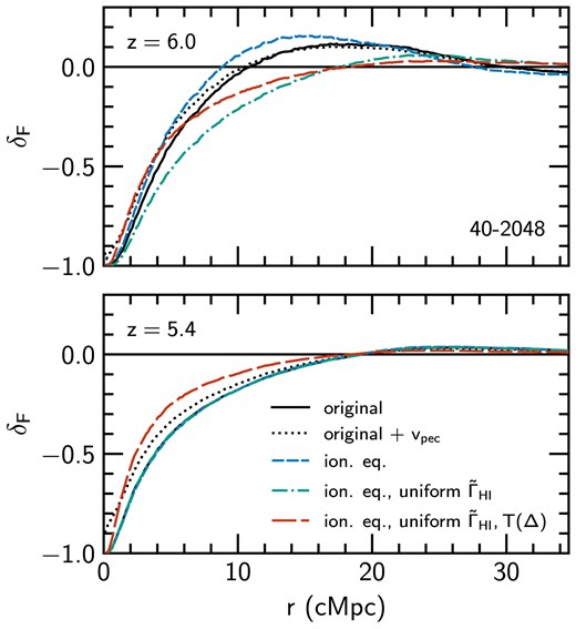
Galaxy–Ly |$\alpha$| transmission correlation calculated from the 40–2048 run (‘original’, black solid), after: recomputing the ionization fractions of hydrogen and helium assuming ionization equilibrium (‘ion. eq.’, blue short dashed); setting the photoionization rate to be uniform (‘ion. eq., uniform |$\tilde{\Gamma }_{\rm H\,I}$|’, green dot–dashed); and after removing temperature fluctuations by setting |$T\propto \Delta ^{\gamma -1}$| and rescaling the neutral fraction appropriately (‘ion. eq., uniform |$\tilde{\Gamma }_{\rm H\,I}$|, |$T(\Delta)$|’, red long dashed). Also shown is the original case including peculiar velocities (‘original + |$v_{\rm pec}$|’, black dotted)–all other curves do not include the effect of peculiar velocities on Ly |$\alpha$| transmission. We show results at |$z=6$| (top panel) and |$z=5.4$| (bottom panel). Note that at |$z=5.4$| the curves lie directly on top of one another, except for the ‘original + |$v_{\rm pec}$|’ and ‘ion. eq., uniform |$\tilde{\Gamma }_{\rm H\,I}$|, |$T(\Delta)$|’ cases.
Next we turn to the blue short-dashed curve in Fig. 11 (‘ion. eq.’), which shows |$\delta _F$| calculated from sightlines where the ionic abundances have been recalculated assuming the gas is in ionization equilibrium with the spatially inhomogeneous UV background used in the simulation. Contrasting the blue short-dashed curves with the solid black curves isolates the impact of non-equilibrium effects on |$\delta _F$|. At |$z=5.4$|, non-equilibrium effects have no impact on |$\delta _F$|. This is not surprising, given that reionization has ended and so the gas is already largely in ionization equilibrium. In contrast, non-equilibrium effects play a role in modifying the shape of |$\delta _F$| at |$z=6$|, though qualitatively the picture remains the same (i.e. the excess in |$\delta _F$| remains after enforcing ionization equilibrium). Again, it is not surprising that non-equilibrium effects are important during reionization, because not all of the gas will be in ionization equilibrium. Zhu et al. (2024b) also explore the impact of assuming ionization equilibrium on |$n_{\rm H\,I}$|, finding that it leads to deviations at the few per cent level.
The green dot–dashed curve in Fig. 11 (‘ion. eq., uniform |$\tilde{\Gamma }_{\rm H\,I}$|’) also assumes ionization equilibrium, but this time we do not use the inhomogeneous UV background from the simulation. Instead, we assume that the UV background is spatially uniform with photoionization rate |$\tilde{\Gamma }_{\rm H\,I}$|. Comparing the green dot–dashed and blue short-dashed curves therefore highlights the importance of UV background fluctuations due to patchy reionization. For |$\tilde{\Gamma }_{\rm H\,I}$| we use the time-varying, average photoionization rate measured at a distance of |$1.5~{\rm cMpc}$| away from all haloes with |$M_{\rm h} \ge 10^{10}~h^{-1}\, {\rm M}_\odot$| in the fiducial 40–2048 simulation. The exact value of |$\tilde{\Gamma }_{\rm H\,I}$|, or the distance at which it is measured, is of little import – the key point is that |$\tilde{\Gamma }_{\rm H\,I}$| must be large enough to induce small enough equilibrium values of |$x_{\rm H\,I}$| to allow for Ly |$\alpha$| transmission; at |$z=6$| (|$z=5.4$|) |$\tilde{\Gamma }_{\rm H\,I}=2.0\times 10^{-13}~{\rm s}^{-1}$| (|$3.2\times 10^{-13}~{\rm s}^{-1}$|). At |$z=6$|, the effect of the uniform UVB is striking. The large excess in |$\delta _F$| around |$10\lesssim r/{\rm cMpc} \lesssim 25$| is no longer present. Instead, the |$z=6$| green dot–dashed curve most closely resembles its post-reionization counterpart at |$z=5.4$|, where the shape of |$\delta _F$| is characterized by |$\delta _F< 0$| for |$r\lesssim 20~{\rm cMpc}$|. From this, we infer that the excess in |$\delta _F$| present in the original simulation is a direct consequence of the inhomogeneous nature of reionization, i.e. the excess is driven by local ionization enhancement due to ionizing sources, or clustered sources. This also highlights the importance of contrast with |$\delta _F$| – if |$\bar{F}$| is small (e.g. due to large neutral fractions in the average IGM) then even a small increase in transmission can lead to a large excess in |$\delta _F$|. At |$z=5.4$|, enforcing a uniform UV background makes no difference to |$\delta _F$|, as the radiation field is already almost entirely uniform (cf. the fluctuations in |$\Gamma _{\rm H\,I}$| in Fig. 3).
Finally, we turn to the red long-dashed curve in Fig. 11 (‘ion. eq., uniform |$\tilde{\Gamma }_{\rm H\,I}$|, |$T(\Delta)$|’), which examines the effect of temperature fluctuations on |$\delta _F$|. To do this, we take the sightlines with a uniform UV background (i.e. the sightlines used to produce the green dot–dashed curve) and fit the relation
to the low-density (|$\Delta < 10$|) ionized (|$x_{\rm HI}< 10^{-3}$|) gas at each z. To remove any effect due to the redshift evolution of |$T_0$| and |$\gamma$|, we fix their value to the average of the |$z=6$| and |$z=5.4$| values, taking |$T_0=1.14\times 10^4~{\rm K}$| and |$\gamma =1.15$|. These parameter values are consistent with the Gaikwad et al. (2020) constraints, which cover almost exactly the same redshift range. We then recalculate the temperature in every pixel using equation (3) and the fitted parameters |$T_0$| and |$\gamma$|, thus removing spatial fluctuations in temperature due to inhomogeneous reionization. The corresponding original neutral fraction |$x_{\rm HI, orig}$| in each pixel is then rescaled, using the original temperature |$T_{\rm orig}$| and assuming photoionization equilibrium, according to
where |$\alpha _A$| is the case-A recombination rate calculated using the fit in Verner & Ferland (1996). At both redshifts, we see that removing temperature fluctuations (red long dashed curves) makes |$\delta _F$| larger (less negative) closer to haloes (|$r\lesssim 15~{\rm cMpc}$|) compared to the case with a uniform UV background and temperature fluctuations (green dot–dashed curves). This is because, in the patchy reionization scenario, gas close to haloes is heated earlier than gas farther away, and therefore has more time to cool (cf. right column of Fig. 3). Setting |$T\propto \Delta ^{\gamma -1}$| and performing the appropriate rescaling of |$x_{\rm H\,I}$| removes these fluctuations and thus reduces the contrast between small r (where gas was initially slightly colder) and large r (where gas was initially slightly warmer), leading to the relative increase in |$\delta _F$| at small r. In the lower panel of Fig. 11, we observe this effect persists after fluctuations in the UV background have faded away (see also Christenson et al. 2023; Gangolli et al. 2024; Garaldi & Bellscheidt 2024b, for the importance of this effect in the context of the connection between Ly |$\alpha$| opacity and galaxy density).
4.3 Relic post-reionization temperature fluctuations
Finally, we explore in more detail how temperature fluctuations affect the post-reionization evolution of |$\delta _F$| at |$4.2\le z \le 5.2$|. To isolate the temperature fluctuations we use the average |$T_0$| and |$\gamma$| in the models over this redshift range to once again remove any effect due to the redshift evolution of these parameters. We use |$T_0=1.14\times 10^4~{\rm K}$| and |$\gamma =1.25$|; this |$\gamma$| is consistent with the Boera et al. (2019) results but |$T_0$| is somewhat larger than that reported in that study.
In Fig. 12, we show the post-reionization evolution of |$\delta _F$| with (solid curves) and without (dashed curves) the post reionization temperature fluctuations, focusing on the region close to the haloes where excess absorption (negative |$\delta _F$|) occurs. The redshift evolution of the excess absorption in the original case is much stronger than in the rescaled |$T(\Delta)$| case, where the evolution is now instead driven almost entirely by the redshift evolution of the mean transmission. Therefore, at these post-reionization redshifts, we expect that relic temperature fluctuations due to inhomogeneous reionization should play a significant role in setting the galaxy–Ly |$\alpha$| transmission correlation in proximity to the haloes hosting ionizing sources. As redshift decreases, the role of temperature fluctuations diminishes (i.e. the original case approaches the |$T(\Delta)$| case). This is in line with predictions from previous studies which have found that the effect of relic temperature fluctuations (due to inhomogeneous reionization) on e.g. the 1D Ly |$\alpha$| forest power spectrum decrease with decreasing redshift (e.g. Molaro et al. 2022). Recent work by Matthee et al. (2024) has begun to probe the excess small-scale Ly |$\alpha$| absorption around galaxies in the post-reionization epoch (|$z\approx 4$|). Extending this work to study the redshift evolution of this excess absorption could therefore provide insights into the nature of post-reionization relic temperature fluctuations, and consequently on the timing of reionization.
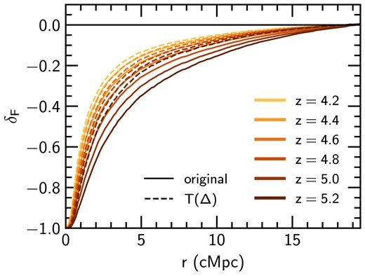
Post-reionization galaxy–Ly |$\alpha$| transmission correlation from the original slightlines (‘original’, solid) and where temperatures have been recalculated according to |$T \propto \Delta ^{\gamma -1}$| to remove spatial fluctuations in the gas temperature and |$x_{\rm H\,I}$| has been appropriately rescaled (‘|$T(\Delta)$|’, dashed), shown from |$z=5.2$| (dark brown) to |$z=4.2$| (gold).
5 CONCLUSIONS
In this work, we have explored the cross-correlation between galaxies and Ly |$\alpha$| transmission in the intergalactic medium, using the Sherwood–Relics simulations (Puchwein et al. 2023). The Sherwood–Relics suite uses a novel hybrid radiative transfer approach, which self-consistently captures the hydrodynamic response of gas to inhomogeneous reionization, and is designed to accurately model the Ly |$\alpha$| forest. Our main findings are as follows:
We find quantitative agreement between the galaxy–Ly |$\alpha$| transmission correlation predicted by Sherwood–Relics model and Meyer et al. (2019) (who use C iv absorbers as a proxy for galaxies) if the galaxies are hosted in haloes with masses |$M_{\rm h}\ge 10^{10}~h^{-1}\, {\rm M}_\odot$|, although only if there is a redshift mismatch between simulation and observation; the agreement occurs for higher redshifts in our models, |$z=6$|, than the average redshift of |$z=5.2$| in the Meyer et al. (2019) measurements (see also Garaldi et al. 2022, for a similar result). However, this redshift mismatch is equivalent to requiring |$\bar{x}_{\rm H\,I}\sim 0.1$| at |$z\simeq 5.2$|, which is inconsistent with the observed Ly |$\alpha$| forest effective optical depth distribution at |$z=5.2$| (Bosman et al. 2022). We suggest this apparent tension may be partly resolved if the minimum C iv absorber host halo mass is instead larger than |$M_{\rm h}=10^{10}~h^{-1}\, {\rm M}_\odot$|, which is still consistent with the C iv bias reported by Meyer et al. (2019). We find poorer agreement with Meyer et al. (2020) and Kashino et al. (2023), although these measurements are more heavily impacted by limited sample size and noise.
We find reasonable quantitative agreement (|$< 1.5 \sigma$|) between the recent [O iii] emitter–Ly |$\alpha$| transmission correlation reported by Kakiichi et al. (2025) at |$z=5.8$| from the JWST ASPIRE survey, but only when using our larger |$160^{3}~h^{-1}\rm \, cMpc^{3}$| simulation volume. The peak in |$\delta _F$| occurs at a smaller |$r\approx 20~{\rm cMpc}$| than in the observational data when selecting haloes with |$M_{\rm h}>10^{10}~h^{-1}\, {\rm M}_\odot$|. Selecting a larger minimum halo mass and/or a larger simulation box size that captures the ionizing source clustering around massive haloes may improve agreement further. By contrast, our smaller simulation volume of |$40^{3}~h^{-3}\rm \, cMpc^{3}$| fails to match the Kakiichi et al. (2025) data at |$r>20~\rm \, cMpc$|.
We also find qualitative agreement between the shape of the galaxy–Ly |$\alpha$| transmission correlation in the Sherwood–Relics models and a variety of measurements of the galaxy–Ly |$\alpha$| transmission correlation at |$z\le 4$|. However, we are unable to perform a direct comparison as our simulation outputs do not extend below |$z=4$|.
The galaxy–Ly |$\alpha$| transmission correlation is sensitive to the volume averaged neutral fraction of the IGM, and is largely insensitive to different reionization histories after accounting for differences in the neutral fraction (at least for the source model used in Sherwood–Relics, which assumes ionising luminosity is proportional to halo mass). However, a partial degeneracy arises from the assumed host halo masses for the galaxies used in the calculation of the correlation. This degeneracy means it may require an independent measure of the host halo masses to use the galaxy–Ly |$\alpha$| transmission correlation as a simple proxy for the IGM neutral fraction.
During reionization, excess transmission around galaxies is driven largely by the enhanced ionizing radiation field due to clustered ionizing sources. Spatial fluctuations in the IGM also play a small role, due to the hotter gas present in recently reionized regions. Non-equilibrium effects only have a modest impact on the galaxy–Ly |$\alpha$| transmission correlation (see e.g. Zhu et al. 2024b). The distance where the peak excess transmission in the cross-correlation occurs is closely related to the the mean free path of Lyman-limit photons around the galaxy host haloes (see also Feron et al. 2024; Garaldi & Bellscheidt 2024a; Fan et al. 2025).
After reionization, for |$r\lesssim 20~{\rm cMpc}$|, relic spatial fluctuations in the IGM temperature affect the shape of the galaxy–Ly |$\alpha$| transmission correlation. As redshift decreases, the strength of this effect decreases, and it should fade by |$z\approx 4$| (e.g. Molaro et al. 2022). The physical explanation is that gas close to haloes is reionized earlier, and thus has more time to cool, in contrast to gas at larger distances which is reionized later and is comparatively hotter. Observations are beginning to probe the galaxy–Ly |$\alpha$| transmission correlation at |$4\lesssim z \lesssim 5$| (Matthee et al. 2024). Constraining the redshift evolution of the correlation over this period, at scales of a |$\sim \text{few~cMpc}$|, could provide complementary insight into the timing of reionization via the signature of post-reionization temperature fluctuations.
In summary, the galaxy–Ly |$\alpha$| transmission correlation is an exciting probe of the connection between high-redshift galaxies and the intergalactic medium, with the potential to offer new insights into the timing and main drivers of reionization. At present, the high-redshift picture is limited by a paucity of data, but current – e.g. the JWST surveys EIGER (Kashino et al. 2023) and ASPIRE (Jin et al. 2024; Kakiichi et al. 2025) – and future observing programmes will shed more light on this promising probe of the tail end of reionization. Additional work on forward modelling of simulations to better reflect the observations (e.g. for the galaxy selection criteria) could prove fruitful (Garaldi & Bellscheidt 2024b). We also suggest that further modelling that explores the impact of different source models (particularly where the relationship between halo mass and ionizing emissivity is varied, e.g. Cain et al. 2023; Asthana et al. 2024b, but see also Garaldi et al. 2022; Garaldi & Bellscheidt 2024a) will be especially useful in linking the properties of ionising sources with the intergalactic medium. Finally, larger volume simulations (|$>160^{3}h^{-3}\, \rm cMpc^{3}$|) with sufficient mass resolution to resolve the Ly |$\alpha$| forest transmission at |$z>5$| will also be valuable for exploring the galaxy–Ly |$\alpha$| correlation on large scales and for galaxy host halo masses |$M_{\rm h}>10^{12}~h^{-1}\, {\rm M}_\odot$|.
ACKNOWLEDGEMENTS
We thank the anonymous referee for a constructive report, and Enrico Garaldi, Koki Kakiichi, Daichi Kashino, and Romain Meyer for insightful discussions and sharing data. The simulations used in this work were performed using the Joliot Curie supercomputer at the Trés Grand Centre de Calcul (TGCC) and the Cambridge Service for Data Driven Discovery (CSD3), part of which is operated by the University of Cambridge Research Computing on behalf of the STFC DiRAC HPC Facility (www.dirac.ac.uk). We acknowledge the Partnership for Advanced Computing in Europe (PRACE) for awarding us time on Joliot Curie in the 16th call. The DiRAC component of CSD3 was funded by BEIS capital funding via STFC capital grants ST/P002307/1 and ST/R002452/1 and STFC operations grant ST/R00689X/1. This work also used the DiRAC@Durham facility managed by the Institute for Computational Cosmology on behalf of the STFC DiRAC HPC Facility. The equipment was funded by BEIS capital funding via STFC capital grants ST/P002293/1 and ST/R002371/1, Durham University and STFC operations grant ST/R000832/1. DiRAC is part of the National e-Infrastructure. LC and JSB were supported by STFC consolidated grant ST/X000982/1. Support by ERC Advanced Grant 320596 ‘The Emergence of Structure During the Epoch of Reionization’ is gratefully acknowledged. MGH was supported by STFC consolidated grants ST/N000927/1 and ST/S000623/1. We thank Volker Springel for making P-Gadget-3 available. We also thank Dominique Aubert for sharing the aton code, and Philip Parry for technical support. This work made use of the following open-source software packages: cmasher (van der Velden 2020); matplotlib (Hunter 2007); numpy (Harris et al. 2020); open-cv (Bradski 2000); and scipy (Virtanen et al. 2020).
DATA AVAILABILITY
All data and analysis code used in this work are available from the first author on reasonable request. Further guidance on accessing the Sherwood–Relics simulation data may also be found at https://www.nottingham.ac.uk/astronomy/sherwood-relics/.
Footnotes
The halo mass bins used to calculate |$\Lambda _{\rm mfp}$| in Feron et al. (2024) are slightly different to those employed here, with a mean halo mass |$\langle M_{\rm h}/h^{-1}\, {\rm M}_\odot \rangle$| of |$10^{10.5}$| at |$z=7$|, |$10^{10.7}$| at |$z=6$| and |$10^{10.9}$| at |$z=5.4$|.
That we are able to reproduce the observed |$\delta _F>0$| for |$r \gtrsim 20~{\rm cMpc}$| in the 160–2048 model, but not the 40–2048 model, suggests that large box sizes (|$L_{\rm box}>40~h^{-1}\, {\rm Mpc}$|) are required to model the signal at these scales. This presents a challenge to theoretical works exploring this effect, given the high resolution simultaneously required to correctly model the Ly |$\alpha$| forest (Bolton & Becker 2009).
Feron et al. (2024) measure |$\Lambda _{\rm mfp}$| from sightlines originating at the virial radius of haloes (see their section 4 for details).
Strictly speaking, the quantity shown is not the halo multiplicity function |$f(\sigma ,z)$|, but is a closely related function, which we plot to reduce the large dynamic range in |${\rm d}n /{\rm d}M$|.
REFERENCES
APPENDIX A: RESOLUTION CONVERGENCE
Fig. A1 shows the halo multiplicity function (e.g. Jenkins et al. 2001)
where |$\sigma ^2$| is the variance of the linear density field, M is halo mass, |$\bar{\rho }_{\rm m}(z)$| is the background matter density at redshift z and |${\rm d}n(M, z)/{\rm d}M$| is the differential halo mass function, for the 40–512, 40–2048, and 160–2048 runs (top panel).6 In the same figure, we also show the ratio of |${\rm d}n/{\rm d}M$| for 40–2048, 40–1024, and 160–2048 to 40–512 (bottom panel), demonstrating – for |$10^{9} \le M_{\rm h}/h^{-1}\, {\rm M}_\odot \le 10^{11}$| – convergence to better than 20 per cent (and mostly better than 10 per cent) for all z with respect to both box size and mass resolution. The smaller volume of the |$40~h^{-1}\, {\rm Mpc}$| runs means that haloes with |$M_{\rm h}> 10^{11}~h^{-1}\, {\rm M}_\odot$| are rarer than in the |$160~h^{-1}\, {\rm Mpc}$| run and, above this mass, the mass functions are clearly not converged with box size or resolution. When making comparisons between runs, we therefore restrict ourselves to haloes with masses |$10^{10} \le M_{\rm h}/h^{-1}\, {\rm M}_\odot \le 10^{11}$|.
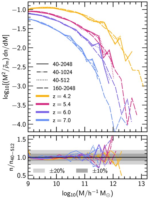
Halo multiplicity functions (top panel) for the 40–2048 (solid), 40–1024 (dot–dashed), 40–512 (dotted), and 160–2048 (long-dashed) runs, at |$z=7.0$| (blue), |$z=6.0$| (purple), |$z=5.4$| (dark pink), and |$z=4.2$| (gold). We also show the ratio of 40–2048, 40–1024, and 160–2048 to 40–512 at each redshift (bottom panel), indicating the 20 per cent and 10 per cent scatter with light and dark grey bands, respectively.
In Fig. A2, we show |$\delta _F$| for the |$40~h^{-1}\, {\rm Mpc}$| Sherwood–Relics realization at three mass resolutions, where the 40–1024 (40-512) run has a particle mass 8 (64) times larger than the 40–2048 run. We compare the three runs at approximately equal volume-averaged neutral fraction |$\bar{x}_{\rm H\,I}$| to eliminate any differences due to slightly different reionization histories. We also note that each run is normalized to the global Ly |$\alpha$| transmission for that run, which is in general different between runs. We find that the form of |$\delta _F$| for our fiducial 40–2048 model is broadly converged with mass resolution.
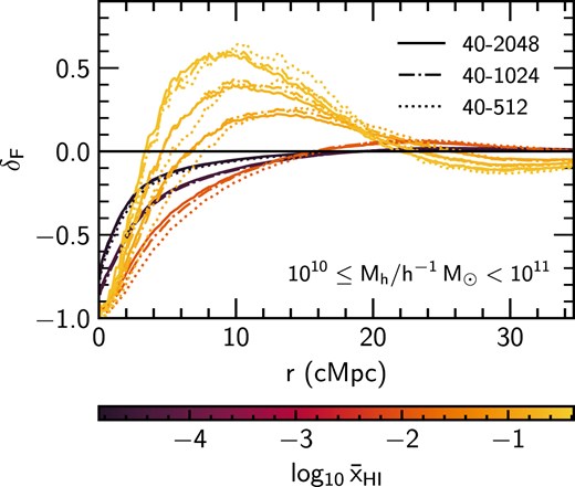
Galaxy–Ly |$\alpha$| transmission correlation as a function of distance r from haloes with mass |$10^{10} \le M_{\rm h}/h^{-1}\, {\rm M}_\odot < 10^{11}$| for different Sherwood–Relics runs, compared at approximately equal volume-averaged neutral fraction |$\bar{x}_{\rm H\,I}$|. We show the fiducial 40–2048 (solid) simulation with the 40–1024 (dot–dashed) and 40–512 (dotted) simulations, which have the same box size of 40 |$h^{-1}\, {\rm Mpc}$| but a particle mass that is 8 and 64 times larger, respectively, demonstrating the impact of mass resolution.
APPENDIX B: GALAXY–TRANSMISSION SPIKE TWO-POINT CROSS-CORRELATION
At high redshifts (|$z \gtrsim 6$|), the transmission in the Ly |$\alpha$| forest decreases to such a degree (see Fig. 1) that it approaches the noise level of spectrographs (|$F\sim 0.02$|, see e.g. fig. 8 in Meyer et al. 2020), making measuring |$\delta _F$| an increasingly difficult task. Meyer et al. (2020) therefore proposed using a slightly different statistic, instead measuring the two-point cross-correlation function (2PCCF) of galaxies and Ly |$\alpha$| transmission spikes. However, what constitutes a transmission spike will depend on many factors, such as the redshift at which the transmission is measured, or the resolution and noise level of the instrument being used. These complications mean we have opted to use |$\delta _F$| in our main analysis, as it can be applied more readily to disparate data sets. Meyer et al. (2020) define a spike as a pixel at |$z\sim 6$| with a signal-to-noise ratio |$>3$| (after convolution with a Gaussian, see their section 3 for details) and |$F>0.02$|. With the spikes identified, Meyer et al. (2020) use the following estimator for the 2PCCF, originally due to Davis & Peebles (1983)
where |$D_{\rm G}D_{\rm S}$| is the number of galaxy-spike pairs as a function of r, |$R_{\rm G}D_{\rm S}$| is the number of random-spike pairs (where the random positions are drawn from a uniform distribution) as a function of r and |$n_{\rm G}$| and |$n_{\rm R}$| are the total numbers of galaxy-spike and random-spike pairs, used for normalization.
In Fig. B1, we show the galaxy-spike 2PCCF measured from our simulations, where we identify spikes as any pixel with |$F>0.02$| and galaxies as haloes with |$M_{\rm h}\ge 10^{10}~h^{-1}\, {\rm M}_\odot$|. We do not model observational effects (e.g. resolution or noise), deferring a study of their impact to future work. We now find excellent agreement between the 160–2048 model and the Meyer et al. (2020) correlation with LBGs (mostly |$< 1\sigma$|) and slightly poorer agreement with their correlation with LAEs. As found in Section 3.2, for |$r \lesssim 20~{\rm cMpc}$| we find excellent agreement (always |$< 1\sigma$|) between the 40–2048 and both the Meyer et al. (2020) LBG and LAE correlations, but poor agreement at larger r. The lack of a redshift mismatch also suggests that the most plausible explanation for the apparent tension with the Meyer et al. (2019) |$\delta _{F}$| measurements is the uncertain C iv absorber bias, rather than differences in the reionization history.
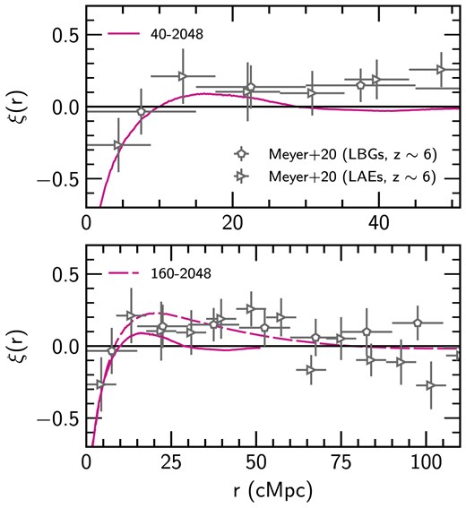
The two-point cross-correlation function between galaxies and transmission spikes at |$z=6$| in the 40–2048 (solid, top and bottom panels) and 160–2048 (dashed, bottom panel) models. Also shown are the constraints due to Meyer et al. (2020) (grey points). Note the different ranges of r between the top and bottom panels.
