


ABSTRACT
We present deep JWST/NIRSpec integral-field spectroscopy (IFS) and ALMA [C ii]|$\lambda $|158|$\mu$|m observations of COS-3018, a star-forming galaxy at z |$\sim$| 6.85, as part of the GA-NIFS programme. Both G395H (R |$\sim$| 2700) and PRISM (R |$\sim$| 100) NIRSpec observations revealed that COS-3018 is comprised of three separate components detected in [O iii]|$\lambda $|5007, which we dub as Main, North, and East, with stellar masses of 10|$^{9.4 \pm 0.1}$|, 10|$^{9.2 \pm 0.07}$|, 10|$^{7.7 \pm 0.15}$| |$\mathrm{M}_\odot$|. We detect [O iii]|$\lambda $||$\lambda $|5007,4959, [O ii]|$\lambda $||$\lambda $|3727,3729, and multiple Balmer lines in all three components together with [O iii]|$\lambda $|4363 in the Main and North components. This allows us to measure an interstellar medium temperature of |$T_\text{e}$| = 1.27|$\pm 0.07\times 10^4$| and |$T_\text{e}$| = 1.6|$\pm 0.14\times 10^4$| K with densities of |$n_{e}$| = 1250|$\pm$|250 and |$n_{e}$| = 700|$\pm$|200 cm|$^{-3}$|, respectively. These deep observations allow us to measure an average metallicity of 12 + log(O/H) = 7.9–8.2 for the three components with the T|$_{e}$|-method. We do not find any significant evidence of metallicity gradients between the components. Furthermore, we also detect [N ii]|$\lambda $|6585, one of the highest redshift detections of this emission line. We find that in a small, metal-poor clump 0.2 arcsec west of the North component, N/O is elevated compared to other regions, indicating that nitrogen enrichment originates from smaller substructures, possibly proto-globular clusters. [O iii]|$\lambda $|5007 kinematics show that this system is merging, which is probably driving the ongoing, luminous starburst.
1 INTRODUCTION
With the launch of JWST, we are now able to observe rest-frame optical and UV emission features, and hence probe the interstellar medium (ISM) of galaxies, up to redshift |$\sim$| 14 (Arribas et al. 2024; Cameron et al. 2023a; Curtis-Lake et al. 2023; Harikane et al. 2023; Hsiao et al. 2024; Isobe et al. 2023b; Larson et al. 2023; Robertson et al. 2023; Tacchella et al. 2023, 2024; Abdurro’uf et al. 2024; Carniani et al. 2024; Sanders et al. 2024; Vikaeus et al. 2024; Harikane et al. 2025).
Before the launch of JWST, the main avenue to study the ISM properties of galaxies at the epoch of reionization (EoR; z |$>$|6) was through [C ii]|$\lambda $|158 |$\mu$|m and [O iii]|$\lambda $|88 |$\mu$|m emission lines and dust continuum observed with mm/sub-mm facilities (mainly ALMA). These observations revealed the early emergence of rotating discs (e.g. Smit et al. 2018; Neeleman et al. 2020; Rizzo et al. 2020, 2021; Fraternali et al. 2021; Lelli et al. 2021; Parlanti et al. 2023; Rowland et al. 2024) and a fast production of dust (e.g. Laporte et al. 2017; Bouwens et al. 2021; Witstok et al. 2022). However, the ISM studies were severely limited by the lack of access to rest-frame optical emission lines as well as the limited detectability of FIR lines by ALMA. JWST has demonstrated its ability to spatially resolve the ISM at very high-z, opening the opportunity to study not only the global properties but also the internal structure of early cosmic systems (e.g. Arribas et al. 2024; D’Eugenio et al. 2024a; Decarli et al. 2024; Lamperti et al. 2024; Rodríguez Del Pino et al. 2024; Jones et al. 2024a; Übler et al. 2024b).
With its unmatched capabilities, NIRSpec (near infrared spectrograph) on board JWST has enabled rapid progress in the physical properties of galaxies at z|$>$|3 when it comes to their abundance (Pérez-González et al. 2023; Harikane et al. 2024b; McLeod et al. 2024; Robertson et al. 2024), detection of active galactic nuclei (AGNs; e.g. Furtak et al. 2024; Greene et al. 2024; Harikane et al. 2023; Kocevski et al. 2023; Maiolino et al. 2024a, b; Matthee et al. 2024; Onoue et al. 2023; Perna et al. 2023; Scholtz et al. 2023b; Übler et al. 2023, 2024a, b), bursty star-formation histories (SFHs; e.g. Tacchella et al. 2023; Dressler et al. 2023; Endsley et al. 2024; Looser et al. 2023; Clarke et al. 2024), discovery of compact galaxies with intense starbursts and/or nuclear activity enshrouded by significant amounts of warm dust (Akins et al. 2024; Casey et al. 2024; Pérez-González et al. 2024b) and ISM conditions (e.g. Cameron et al. 2023a; Reddy et al. 2023; Sanders et al. 2023; Calabro et al. 2024).
JWST observations of high redshift galaxies have revealed metal-poor galaxies with intense star formation, releasing large amounts of ionizing radiation resulting in high ionization parameters (Hirschmann et al. 2023; Curti et al. 2023, 2024b; Tacchella et al. 2023; Trump et al. 2023; Simmonds et al. 2024). Furthermore, the access to deep observations of rest-frame optical and UV emission lines allows astronomers to investigate the abundances of different elements, revealing, in some cases, unexpected ionization and chemical enrichment patterns (e.g. Bunker et al. 2023; Isobe et al. 2023a; Maiolino et al. 2024a; Cameron et al. 2024; D’Eugenio et al. 2024b; Cameron et al. 2023b; Topping et al. 2024; Ji et al. 2024a; Schaerer et al. 2024; Ji et al. 2024c). JWST/NIRSpec has also allowed for significant progress in galaxy kinematics, as we now have access to optical emission lines at z|$>$|3.5 (Nelson et al. 2023; de Graaff et al. 2024; Lamperti et al. 2024; Rodríguez Del Pino et al. 2024; Jones et al. 2024a; Übler et al. 2024b), allowing for a comparison of ionized and cold gas kinematics at high redshift (Parlanti et al. 2023; Lamperti et al. 2024).
In this paper, we present new observations of COS-3018 from the Galaxy Assembly with NIRSpec Integral Field Spectroscopy (GA-NIFS) Guaranteed Time Observations (GTO) programme (e.g. Arribas et al. 2024; D’Eugenio et al. 2024a; Marshall et al. 2023; Perna et al. 2023; Übler et al. 2023, 2024a, b; Ji et al. 2024b; Jones et al. 2024a; Lamperti et al. 2024; Pérez-González et al. 2024a; Rodríguez Del Pino et al. 2024). This survey aims to investigate the spatially resolved stellar populations, ISM, outflow and kinematics properties of 55 quasars, AGN and star-forming galaxies (SFGs) in the redshift range of |$z\sim 2-11$| with NIRSpec IFU, utilising both the PRISM, medium and high spectral resolution observations. In this work, we present spatially resolved gas and stellar populations of COS-3018 using new JWST/NIRSpec Integral Field Unit (IFU) high-resolution grating (R |$\sim$| 2700) and low-resolution prism (R |$\sim$| 100) observations as well as JWST/NIRCam imaging.
COS-3018, a star-forming galaxy at z = 6.85, was first discovered by Smit et al. (2014) by identifying objects with large equivalent width (EW) of [O iii]|$\lambda $||$\lambda $|5007,4959 + H β based on HST and Spitzer/IRAC photometry (EW|$_{\rm rest}>1200~\mathring{\rm A}$|). COS-3018 has been intensively studied using both ground-based near-infrared (NIR) spectroscopy and ALMA. Laporte et al. (2017) used VLT/X-shooter (Vernet et al. 2011) to detect C iii]|$\lambda $||$\lambda $|1907,1909 emission, without any detection of Ly α or higher ionization lines like He ii|$\lambda $|1640 and C iv|$\lambda $||$\lambda $|1548,1551. ALMA observations of [C ii]|$\lambda $|158 |$\mu$|m emission lines revealed a velocity gradient in the system, suggesting an established cold rotating disc at these early epochs (Smit et al. 2018), later confirmed by Parlanti et al. (2023) as a turbulent disc with high-velocity dispersion. Vallini et al. (2020) studied the ISM conditions in COS-3018 using C iii]|$\lambda $||$\lambda $|1907,1909, [C ii]|$\lambda $|158 |$\mu$|m and [O iii]|$\lambda $|88 |$\mu$|m observations, inferring a high metallicity of |$\sim 0.4$| Z|$_{\odot }$| and an ISM density of |$\sim 500$| cm|$^{-3}$|. Witstok et al. (2022) further analysed the ALMA dust continuum and integrated emission line properties to constrain the dust temperature of |$\sim$|30–40 K, resulting in a high dust mass of 2–26|$\times 10^{7}$| |$\mathrm{M}_\odot$|. This dust mass measurement implies a dust-to-stellar mass ratio of 5 per cent, challenging theoretical models to create this much dust by such a high redshift. COS-3018 was observed by the PRIMER programme covering the target with NIR imaging with JWST/NIRCam instrument. Harikane et al. (2025) showed the COS-3018 is composed of multiple UV clumps with a total stellar mass estimated at |$\sim 10^{9.6}$| |$\mathrm{M}_\odot$|.
The paper is structured as follows. In Section 2, we present the JWST/NIRSpec, NIRCam, and ALMA observations, as well as data reduction of each of the data sets. In Section 3, we describe the detailed analysis of each of the observations. In Section 4, we present and discuss our findings and in Section 5 we summarize the results of this work. Throughout this work, we adopt a flat |$\Lambda $|CDM cosmology: H|$_0$|: 67.4 km s|$^{-1}$| Mpc|$^{-1}$|, |$\Omega _\mathrm{m}$| = 0.315, and |$\Omega _\Lambda $| = 0.685 (Planck Collaboration VI 2020).
2 OBSERVATIONS AND DATA REDUCTION
2.1 NIRSpec data
We observed COS-3018 with JWST/NIRSpec in IFS mode (Böker et al. 2022; Jakobsen et al. 2022) as part of the GA-NIFS survey (PID 1217, PIs: S. Arribas & R. Maiolino). The NIRSpec data were taken on 5th of May 2023, with a medium cycling pattern of eight dither positions and a total integration time of 18.2 ks (5.05 h) with the high-resolution grating/filter pair G395H/F290LP, covering the wavelength range |$2.87-5.27~\mu$|m (spectral resolution |$R\sim 2000-3500$|; Jakobsen et al. 2022), and 3.9 ks (1.1 h) with PRISM/CLEAR (|$\lambda =0.6-5.3~\mu$|m, spectral resolution |$R\sim 30-300$|).
Raw data files of these observations were downloaded from the Barbara A. Mikulski Archive for Space Telescopes (MAST) and then processed with the JWST Science Calibration pipeline1 version 1.11.1 under the Calibration Reference Data System (CRDS) context jwst_1149.pmap. We made several modifications to the default reduction steps to increase data quality, which are described in detail by Perna et al. (2023) and which we briefly summarize here. Count-rate frames were corrected for |$1/f$| noise through a polynomial fit. Furthermore, we removed regions affected by failed open MSA shutters during calibration in Stage 2. We also removed regions with strong cosmic ray residuals in several exposures. Any remaining outliers were flagged in individual exposures using an algorithm similar to lacosmic (van Dokkum 2001): we calculated the derivative of the count-rate maps along the dispersion direction, normalized it by the local flux (or by three times the rms noise, whichever was highest), and rejected the 95th percentile of the resulting distribution (see D’Eugenio et al. 2024a, for details). The final cubes were combined using the ‘drizzle’ method. The main analysis in this paper is based on the combined cube with a pixel scale of |$0.05^{\prime \prime }$|.
2.2 ALMA data
In this work, we use the ALMA programme 2018.1.00429.S, which contains higher resolution observations of [C ii]|$\lambda $|158 |$\mu$|m emission line. The data were calibrated and reduced with the automated pipeline of the Common Astronomy Software Application (casa; McMullin et al. 2007) version 5.6. We exclude two service blocks of the programme, as they were taken with significantly shorter baselines and hence giving a resolution of |$\sim 0.5^{\prime \prime }$|, giving a worse resolution in the combined reduced data
The data calibration of the ALMA data was performed using CASA v6.5.4. First, we subtract the continuum from the data using the uvcontsub task. We fit a linear model to the uv-visibilities using the channels without any emission-line contamination. We imaged the continuum-subtracted [C ii]|$\lambda $|158|$\mu$|m visibilities and the dust continuum using tclean at 0.03 arcsec pixel scale using two separate weighting schemes. We first imaged the data using natural weighting to get the total flux from the [C ii]|$\lambda $|158 |$\mu$|m. This results in a final beam size of 0.45|$\times 0.5^{\prime \prime }$|. We created a further data set using the Briggs weighting scheme with a robust parameter of 0.5. This resulted in a high-resolution data set with a beam size of 0.25|$\times 0.3^{\prime \prime }$|. The dust-continuum maps and [C ii]|$\lambda $|158 |$\mu$|m emission line cubes were cleaned down to 3|$\sigma$| with a 3 arcsec circular mask on COS-3018.
The [C ii]|$\lambda $|158 |$\mu$|m emission line cube was analysed using Spectral cube python library. We created zeroth, first, and second-order [C ii]|$\lambda $|158 |$\mu$|m maps by collapsing the cube along the velocity range of −200–200 km s|$^{-1}$|(i.e. |$\pm$|FWHM of the [C ii]|$\lambda $|158 |$\mu$|m emission line) centred on the systematic redshift of the [C ii]|$\lambda $|158 |$\mu$|m emission line.
2.3 NIRCam imaging
We use additional JWST/NIRCam imaging taken as a part of the PRIMER programme2 (PID 1837; PI J. Dunlop). These data consist of imaging in eight NIRCam bands (F090W, F115W, F150W, F200W, F277W, F356W, F410M, and F444W) and we show the RGB image in top panel of Fig. 1. The NIRCam images and photometry were obtained from the DAWN JWST Archive. These data were reduced using a combination of the jwst and grizli3 pipelines (Valentino et al. 2023).
![Overview of the COS-3018 system. Right from top to bottom: RGB image from JWST/NIRCam imaging (with B – F115W, G-F200W, R-F444W filters), [O iii]$\lambda $5007 and H α; maps from R2700 NIRSpec/IFS cube. The coloured dashed line contours indicate the regions used to extract the NIRSpec/PRISM spectra on the left. Left column: Full NIRSpec/PRISM spectra extracted from the NIRSpec/IFU observations in black line. We overlay the NIRCam photometry (from the dashed line apertures) as red points with the NIRCam transmission curve as various coloured shaded regions.](https://oup.silverchair-cdn.com/oup/backfile/Content_public/Journal/mnras/539/3/10.1093_mnras_staf518/2/m_staf518fig1.jpeg?Expires=1750231692&Signature=XSeFii1enmtN5UJWpxbHbR6KDkoyKbTNaCjyMoEy5mIsLS8Cxo4JXRDti1n~wuvuovuFV7vEKPUC3u9K1-IdPjwTBkwo7PxEINmX6AQ2R4AY9IjqiEWXiBr0czzYHjTkD6hFa6K0NJkqUrez7W8LtEPRTxS6l0owZTdJJ-J2mm~dCl5vUgMnb6MPu~qIoUREDJ-Pl18u2~xvCF5ME-9twUApu7ZtFLop1MNB0A8LhbMz5m-A-l8Ua0WO56r3Lb3OwG8yQlm2mwOwSv9x6P7Zpdq8lorh3R0MuZwKWEzHj-Ko5yLuUtzRnHCNKpllpWJq1WHuoSVoeXAy9W9G0jaL-w__&Key-Pair-Id=APKAIE5G5CRDK6RD3PGA)
Overview of the COS-3018 system. Right from top to bottom: RGB image from JWST/NIRCam imaging (with B – F115W, G-F200W, R-F444W filters), [O iii]|$\lambda $|5007 and H α; maps from R2700 NIRSpec/IFS cube. The coloured dashed line contours indicate the regions used to extract the NIRSpec/PRISM spectra on the left. Left column: Full NIRSpec/PRISM spectra extracted from the NIRSpec/IFU observations in black line. We overlay the NIRCam photometry (from the dashed line apertures) as red points with the NIRCam transmission curve as various coloured shaded regions.
3 DATA ANALYSIS
3.1 IFS data and emission line fitting
Before we can analyse the emission line cube of the PRISM or R2700 observations, we first need to perform a few preparatory steps: (1) masking of any outlier pixels not flagged by the pipeline; (2) background subtraction; (3) estimating the uncertainties on the data. For these tasks and the rest of the analysis, we use QubeSpec, an analysis pipeline written for NIRSpec/IFS data.
We need to mask any major pixel outliers that were not flagged by the data reduction pipeline. Although these pixels do not cause significant problems during the emission line fitting of galaxy-integrated spectra, these outliers can become a problem during spaxel-by-spaxel fitting. To identify the residual outliers not flagged by the pipeline, we used the error extension of the data cube. We flagged any pixels whose error is 10|$\times$| above the median error value of the cube. We verified that this does not have any impact on the emission line maps by using the 5 and 20 thresholds without any changes to our conclusions.
For both the PRISM and R2700 observations, we need to subtract the strong background affecting our observations. For the R2700 observations, we mask the location of the source based on its [O iii]|$\lambda $|5007 emission (|$2\sigma$| SNR contours), and we estimate the background using astropy.photutils.background.Background2D (2D background estimator) task with 5|$\times$|5 spaxels box window, for each individual channel in the data cubes. We visually inspected the resulting background spectra and found no evidence of narrow features (e.g. emission or absorption lines). Therefore, to reduce noise, we smoothed the background in spectral space using a median filter with a width of 25 channels to reduce any noise effects. The final estimated background is subtracted from the flux data cube.
The strong background in the PRISM observations requires subtraction of the background on the detector images and we employ the method described in Marconcini et al. (2024). Here, we briefly describe the procedure. The background in the PRISM observations is subtracted from the detector images for each of the dithers. Similarly to the R2700, we create a source mask based on the [O iii]|$\lambda $|5007 emission line with additional padding of 3 pixels. This mask is then deprojected to the 8 detector images, using the blot function in the JWST pipeline. For each of the 2-d calibrated images, we fit the linear function to each of the slices in the dispersion direction, excluding the source pixels defined by our source mask. To filter out noisy features in the background, the estimated background is smoothed by a median filter with a width of 7 pixels. The final background-subtracted cube is constructed using the stage 3 pipeline step from the background-subtracted 2D images.
Übler et al. (2023) reported that the uncertainties on the flux measurements in the ERR extension of the data cubes are underestimated, compared to the noise estimated from the rms of the spectrum, calculated inside spectral window free from emission lines. However, the error extension still carries information about the relative uncertainties between pixels and outliers. Therefore, when extracting each spectrum, whether it is a combined spectrum of multiple spaxels or directly fitting a spaxel, we first retrieve the uncertainty from the error extension. Then we scale this error extension uncertainty so that the error extension’s median uncertainty matches the spectrum’s sigma-clipped rms in emission line-free regions. This scaling is performed across both detectors independently, without a wavelength dependence.
3.1.1 R2700 emission line fitting
We initially fitted the integrated aperture R2700 spectra of the individual components (see Fig. 2 and Section 4) as a series of Gaussian profiles for emission lines and power law to describe the continuum, using the Fitting routines in QubeSpec code. In total we fit the following emission lines: H α, H |$\beta$|, H |$\gamma$|, H |$\delta$|, [N ii]|$\lambda $||$\lambda $|6550,6585, [O iii]|$\lambda $||$\lambda $|5007,4959, [O ii]|$\lambda $||$\lambda $|3727,3729, [Ne iii]|$\lambda $||$\lambda $|3869,3968, He ii|$\lambda $|4686, and HeI|$\lambda $|5875. We use a single Gaussian per emission line as our main model. We tie the redshift (centroid) and intrinsic FWHM of each Gaussian profile to a common value to reduce the number of free parameters, leaving the flux of each Gaussian profile free. For each emission line, the FWHM of the line is convolved with the line spread function of NIRSpec from the JDOCS.4
![Overview of the COS-3018 system. Right from top to bottom: RGB image from JWST/NIRCam imaging (with B – F115W, G-F200W, R-F444W filters), [O iii]$\lambda $5007 and H αmaps from R2700 NIRSpec/IFS cube. The coloured dashed line boxes indicate the regions used to extract the NIRSpec/R2700 spectra on the left. Left column: Full R2700 spectra extracted from the NIRSpec/IFU observations in black line.](https://oup.silverchair-cdn.com/oup/backfile/Content_public/Journal/mnras/539/3/10.1093_mnras_staf518/2/m_staf518fig2.jpeg?Expires=1750231692&Signature=p8mj8r4E-QFuRm6S21e-VKRwIqRZp56sqjEtv4smKL2vk-c-RtzSWH-Mh~ILia9ja5mn7M80cypExdUjYsMllUPOsS0M~Tzk-HQZ9LHaBTZoMh~hlpX1oe9oOYP-SjHEwjrUNkCvtCPZdYp4bUPXEI42fNnz-CKWbYqyYs57IqAwRn~rO-nniZ3GCuGxIxDnk~TOEQ14Ht4ecFCCDzOGKOd61IG3ELLzZpNKmg7f2EFH6duqvgliPPnIsKjPIQE6qK~YjmGXNpA9kEEoTmJKsukBrNH1646Gw8olqaoAum2sagB4LmhUTbyfqbD7DgAVcB6sRi01YZYPp4CYBUSOpQ__&Key-Pair-Id=APKAIE5G5CRDK6RD3PGA)
Overview of the COS-3018 system. Right from top to bottom: RGB image from JWST/NIRCam imaging (with B – F115W, G-F200W, R-F444W filters), [O iii]|$\lambda $|5007 and H αmaps from R2700 NIRSpec/IFS cube. The coloured dashed line boxes indicate the regions used to extract the NIRSpec/R2700 spectra on the left. Left column: Full R2700 spectra extracted from the NIRSpec/IFU observations in black line.
We fixed the [O iii]|$\lambda $|5007/[O iii] [4959] flux ratio to be 2.99 (Dimitrijević et al. 2007); and [N ii]|$\lambda $|6583/[N ii]|$\lambda $|6548 to 3.06 (based on the atomic transition probability; Osterbrock & Ferland 2006). Lastly the [O ii]|$\lambda $|3727/[O ii]|$\lambda $|3729 to vary between 0.69 and 2.6 to reflect the dependence of such doublet on the electron density (Sanders et al. 2016).
Furthermore, each spectrum is also fitted with a 2-Gaussian model, which includes an additional Gaussian profile in H α, H|$\beta$|, and [O iii]|$\lambda $||$\lambda $|5007,4959 emission lines. We only fit an additional ‘narrow-2’ component in these strong emission lines, because they are the only lines with sufficient signal-to-noise ratio to detect non-Gaussian line profiles arising from complex kinematics or outflows. We will further discuss this additional component in Sections 4.5 and 4.6. We use the BIC5 to choose whether the fit needs a second narrow component (using |$\Delta$|BIC |$>10$| as a boundary for choosing a more complex model).
The fiducial model parameters for the single and multicomponent models are estimated with a Bayesian approach, where the posterior probability distribution is calculated using the Markov-Chain Monte Carlo (MCMC) ensemble sampler – emcee (Foreman-Mackey et al. 2013). For each of the variables, we need to define set priors for the MCMC integration. The prior on the redshift of each spectrum is set as a truncated Gaussian distribution, centred on the systemic redshift of the galaxy with a sigma of 300 km s|$^{-1}$| and boundaries of |$\pm 1000$| km s|$^{-1}$|. The prior on the intrinsic FWHM of the narrow-line component is set as a uniform distribution between 100 and 500 km s|$^{-1}$|, while the prior on the amplitude of the line is set as a uniform distribution in logspace between 0.5|$\times$|rms of the spectrum and the maximum of the flux density in the spectrum. For the second Gaussian component in the strong emission lines, the velocity offset is set as a truncated Gaussian distribution with mode 0 and with a sigma of 250 km s|$^{-1}$| and boundaries of |$\pm$|1000 km s|$^{-1}$|, while for the FWHM of the outflow component, we use a uniform distribution with boundaries of 500–2000 km s|$^{-1}$|.
The final best-fitting parameters and their uncertainties are calculated as median value and 68 per cent confidence interval of the posterior distribution. We note that all the quantities derived from R2700 spectral fitting (e.g. gas densities, temperatures, outflow velocities, and metallicities) are calculated from the posterior distribution to account for any correlated uncertainties in the spectrum.
We repeat the spectral fitting on spaxel-by-spaxel in the region covered by the target, using the same models as for the integrated spectra described above. We do not do any PSF matching or spaxel binning at this point. As outlined above, the [O iii]|$\lambda $||$\lambda $|5007,4959, H α and H β have a complex emission line profile which requires multiple Gaussian profiles. In order to describe the emission line profile we use a non-parametric description of the emission line profile: v10, v50 v90, and W80 parameters described as velocity containing 10, 50, 90 per cent of the flux and velocity width containing 80 per cent of the flux (v90–v10), respectively. We will use the W80 parameter to describe velocity dispersion of the emission line profile.6 We show the final derived spatially resolved flux maps in Fig. 3 and kinematics in Figs 4 and 9. We note that the kinematics map are the same if we fit all lines simultaneously or we fit [O iii]|$\lambda $|5007 and H α separately.
![Resolved emission line maps of COS-3018 and derived ISM physical properties from the R2700 NIRSpec IFs cube. In each map, we also show the Main, North, and East components as green, purple, and light blue contours, respectively. Top row: Forbidden lines detected in COS-3018 from left to right:[O iii]$\lambda $$\lambda $5007,4959, [O ii]$\lambda $$\lambda $3727,3729, [Ne iii]$\lambda $$\lambda $3869,3968 and [N ii] emission lines. Middle row: detected Balmer lines in the target: H α H$\beta$, H$\gamma$, and H$\delta$. We also detect He i line in the combined spectra; however, we do not detect it in the individual spaxel spectra. Bottom row: Spatially resolved ISM properties from the strong emission lines, from left to right: Metallicity from strong line calibrations, dust attenuation (from H α and H β) and electron density. The cyan hatched region indicates the size of JWST/NIRSpec PSF at the wavelength of the emission line.](https://oup.silverchair-cdn.com/oup/backfile/Content_public/Journal/mnras/539/3/10.1093_mnras_staf518/2/m_staf518fig3.jpeg?Expires=1750231692&Signature=pYdtXhEzKKbVsWzOHuehrpMoYrjWc53TUIR1cub60aXosAtkUYnY4EElZ4SbsFLsQTQjYbLQpCH3ul-oLKyiFZ-JLVjgVVzkeoHIx255NzIq2K~t4lN7gH5RLxHGwY9ki1yAHo3D76EEPC6VhxCNnu7g6UNWsFnx2K~nT5MqEZVyCZPvMzqUP9RidV8FQw6pr-NG~ttusKw2Dr7VQL6ClPEPornUVwKFdbF4E5NDMOC67mxWj0hCdXqNaxtGPksBb5fJw3prQobbiosRXNQJPVi2tfVNvWZyKim3TPK7wMEyFZgITczVJ-PKJkYlxsH-IduVLI7dNQmBhVvu-cnxQw__&Key-Pair-Id=APKAIE5G5CRDK6RD3PGA)
Resolved emission line maps of COS-3018 and derived ISM physical properties from the R2700 NIRSpec IFs cube. In each map, we also show the Main, North, and East components as green, purple, and light blue contours, respectively. Top row: Forbidden lines detected in COS-3018 from left to right:[O iii]|$\lambda $||$\lambda $|5007,4959, [O ii]|$\lambda $||$\lambda $|3727,3729, [Ne iii]|$\lambda $||$\lambda $|3869,3968 and [N ii] emission lines. Middle row: detected Balmer lines in the target: H α H|$\beta$|, H|$\gamma$|, and H|$\delta$|. We also detect He i line in the combined spectra; however, we do not detect it in the individual spaxel spectra. Bottom row: Spatially resolved ISM properties from the strong emission lines, from left to right: Metallicity from strong line calibrations, dust attenuation (from H α and H β) and electron density. The cyan hatched region indicates the size of JWST/NIRSpec PSF at the wavelength of the emission line.
![Kinematics of the [O iii]$\lambda $5007 emission for the narrow-1 and narrow-2 components shown in left and right columns, respectively. From top to bottom: Flux, velocity, and FWHM for each of the components. Velocity maps are calculated relative to the redshift of the Main component. In each map, we also show the Main, North, and East components as green, purple, and light blue contours, respectively. The cyan hatched ellipse indicate the JWST/NIRSpec PSF at the wavelength of the [O iii]$\lambda $5007. [O iii]$\lambda $5007 and the H α have the same kinematics when fitted independently.](https://oup.silverchair-cdn.com/oup/backfile/Content_public/Journal/mnras/539/3/10.1093_mnras_staf518/2/m_staf518fig4.jpeg?Expires=1750231692&Signature=k97eRiOcgUh7D~8q1KmYBu~12qwhMzpNY5YGSg0CmyymXS89lBGxQ6SMS6AkQBjJ8gWq8Ws0d018qt8oUFRUR8opnumFopU4Zl0-Jdnybp9wRV5kvXzjd9OALsuUji3CIwJSMnWnxzMEq5cD96JfflGmIsC1ZTXArRW6XyZ0XjMoLYJ-Th7efWkToOpn-RzN5X0Ym0kPZ9bs-hqM7cKMxhAUhap45s37cMRRbgxrj8k2-ejpyRbmRP8Lc~5vofzV4HupRk7YL2thVZSE1BxUR3Ex4tfrgssrzvpWZ8dJrAyqeJ17nE8GHyCfPr~3iHOm75npV84p62Moya5vjzfqaA__&Key-Pair-Id=APKAIE5G5CRDK6RD3PGA)
Kinematics of the [O iii]|$\lambda $|5007 emission for the narrow-1 and narrow-2 components shown in left and right columns, respectively. From top to bottom: Flux, velocity, and FWHM for each of the components. Velocity maps are calculated relative to the redshift of the Main component. In each map, we also show the Main, North, and East components as green, purple, and light blue contours, respectively. The cyan hatched ellipse indicate the JWST/NIRSpec PSF at the wavelength of the [O iii]|$\lambda $|5007. [O iii]|$\lambda $|5007 and the H α have the same kinematics when fitted independently.
![Optical emission line diagnostics sensitive to the source of ionization in COS-3018. Left: N2-R3 BPT ([N ii]/H α versus [O iii]/H β; top row). We show the demarcation lines between star formation and AGNs from Kewley et al. (2001), Kauffmann et al. (2003), and Scholtz et al. (2023b) as black dashed, dotted, and green dash dotted lines, respectively. Middle: He2-N2 (He ii$\lambda $4686/H β versus [N ii]/H α) diagram The black dashed line indicates a demarcation line between star-forming and AGN galaxies by Shirazi & Brinchmann (2012). The black contours show the star-forming galaxies and AGNs from SDSS, respectively. Right panel: [O iii]$\lambda $4363/H $\gamma$ versus [O iii]$\lambda $5007[O ii]$\lambda $$\lambda $3727,3729. The black dashed line indicates the demarcation line from Mazzolari et al. (2024). In each panel, we show ionization models from Feltre, Charlot & Gutkin (2016) and Gutkin, Charlot & Bruzual (2016) as yellow and light blue points, respectively. The magenta and cyan squares show a stacked spectrum for AGNs and star-forming galaxies from Scholtz et al. (2023b).](https://oup.silverchair-cdn.com/oup/backfile/Content_public/Journal/mnras/539/3/10.1093_mnras_staf518/2/m_staf518fig5.jpeg?Expires=1750231692&Signature=zVxtwvWTbh0HUgc3610KnqOOtPftQhvOOE7HCFlcbmganjkTQmb05-fnzIxL3WV8e~1O3ZPmB8O4I41U75svBTeNgTnteMnEzATkSeoNg4l442oKI8kIcj3Rtowf9JbwMN0a8kmDZk3QyQDDdQES1D3GkkDAuU~pXuYLuYclgnPj~0kX28MW1Jhw~hSFMcYQLlVJ1pWi9ziQGmBrvZtWZzmQ2xxsqdv7zu1rZl93EApn6aHDJOyR8JtLzGLvTSdEdTR2Pn~ictkCgl7Pm6UhUoF0NguUOl3Ny9Q-38mYr2YSVBx4jEn9LW6dPTJ5Wpqwby-iWAiUtS7lezny41x9iw__&Key-Pair-Id=APKAIE5G5CRDK6RD3PGA)
Optical emission line diagnostics sensitive to the source of ionization in COS-3018. Left: N2-R3 BPT ([N ii]/H α versus [O iii]/H β; top row). We show the demarcation lines between star formation and AGNs from Kewley et al. (2001), Kauffmann et al. (2003), and Scholtz et al. (2023b) as black dashed, dotted, and green dash dotted lines, respectively. Middle: He2-N2 (He ii|$\lambda $|4686/H β versus [N ii]/H α) diagram The black dashed line indicates a demarcation line between star-forming and AGN galaxies by Shirazi & Brinchmann (2012). The black contours show the star-forming galaxies and AGNs from SDSS, respectively. Right panel: [O iii]|$\lambda $|4363/H |$\gamma$| versus [O iii]|$\lambda $|5007[O ii]|$\lambda $||$\lambda $|3727,3729. The black dashed line indicates the demarcation line from Mazzolari et al. (2024). In each panel, we show ionization models from Feltre, Charlot & Gutkin (2016) and Gutkin, Charlot & Bruzual (2016) as yellow and light blue points, respectively. The magenta and cyan squares show a stacked spectrum for AGNs and star-forming galaxies from Scholtz et al. (2023b).
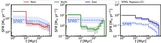
Star formation histories of the three clumps in COS-3018. From left to right: Main, North, and East components, respectively. The time in the x-axis is defined from start of the SFH, with t = 0 Myr corresponds to the redshift of the source. We plot the star-forming main sequence from Popesso et al. (2023) as a blue dashed line for comparison. The Main and North components are going through a major starburst, being |$\sim$|10 higher than the main sequence.
![Top: location of COS-3018 on mass–metallicity relation (MZR). The green, magenta, and blue points show Main, North, and East components for metallicity measurement using T$_{e}$ (squares) and strong line calibration (circles) methods. The orange and dark blue triangles show JWST metallicity measurements of JWST galaxies from Curti et al. (2023). The blue solid line and the shaded region indicate the mass–metallicity relation at z $>$3 (Curti et al. 2023). The black solid line shows the mass–metallicity relation from SDSS at z = 0.07 (Curti et al. 2020). The light blue and green stars show Blueberries and Greenpeas from Yang et al. (2017a, b). Bottom: Comparison of oxygen and nitrogen abundance of different components of COS-3018. The red, blue, gold, and purple squares show the Main, North components, Main-[N ii] and North-[N ii] clumps, respectively. The circles show data from JWST (Isobe et al. 2023b; Cameron et al. 2023b; Castellano et al. 2024; Topping et al. 2024; Curti et al. 2024a; Ji et al. 2024b). The triangles show comparison of local data H ii regions (Tsamis et al. 2003; Esteban et al. 2004, 2009, 2014, 2017; García-Rojas et al. 2004, 2005, 2007; Peimbert, Peimbert & Ruiz 2005; García-Rojas & Esteban 2007; López-Sánchez et al. 2007; Toribio San Cipriano et al. 2016, 2017); local dwarfs (Berg et al. 2016; Vale Asari et al. 2016; Senchyna et al. 2017; Berg et al. 2019).](https://oup.silverchair-cdn.com/oup/backfile/Content_public/Journal/mnras/539/3/10.1093_mnras_staf518/2/m_staf518fig7.jpeg?Expires=1750231692&Signature=ZsWTwQphFwqmtij7T4g7qaXy7rF2VGcUK~MdXpMRtt83lAifjSdDX2UAByVM-~57CrneHLypf7FeMW0Oe~EfQ9sDwoA0ydlUsje4BKB4-B5v36uEbeTLljbz9SPNlWNmIhZsiQNE7BS1gDlXp-q4Bsd2ZjrjF4Z23Ms~Jd7iCR3SGpvq1Aq7bplJPbkeZ~~ACyf64wTLAXjNrwrml8I8luMSBOSz~YrT~y99Yy0KzuQ~mJ3n3kn4Nn26gOCZK27dKQx2RDA3W-9ixHQZvrtjOz2jyTeDCGM-7w-Mif9r3eLDX4Wg2q6A6Ci5xBIOSIsuRWNrx-23LJo4xKvyzHYcfg__&Key-Pair-Id=APKAIE5G5CRDK6RD3PGA)
Top: location of COS-3018 on mass–metallicity relation (MZR). The green, magenta, and blue points show Main, North, and East components for metallicity measurement using T|$_{e}$| (squares) and strong line calibration (circles) methods. The orange and dark blue triangles show JWST metallicity measurements of JWST galaxies from Curti et al. (2023). The blue solid line and the shaded region indicate the mass–metallicity relation at z |$>$|3 (Curti et al. 2023). The black solid line shows the mass–metallicity relation from SDSS at z = 0.07 (Curti et al. 2020). The light blue and green stars show Blueberries and Greenpeas from Yang et al. (2017a, b). Bottom: Comparison of oxygen and nitrogen abundance of different components of COS-3018. The red, blue, gold, and purple squares show the Main, North components, Main-[N ii] and North-[N ii] clumps, respectively. The circles show data from JWST (Isobe et al. 2023b; Cameron et al. 2023b; Castellano et al. 2024; Topping et al. 2024; Curti et al. 2024a; Ji et al. 2024b). The triangles show comparison of local data H ii regions (Tsamis et al. 2003; Esteban et al. 2004, 2009, 2014, 2017; García-Rojas et al. 2004, 2005, 2007; Peimbert, Peimbert & Ruiz 2005; García-Rojas & Esteban 2007; López-Sánchez et al. 2007; Toribio San Cipriano et al. 2016, 2017); local dwarfs (Berg et al. 2016; Vale Asari et al. 2016; Senchyna et al. 2017; Berg et al. 2019).
![Modelling the emission line profile of the [O iii]5007, H $\beta$, and H α to identify any broad outflow components in the Main component. Top panel: The spectrum of the Main component and the best-fitting model. The data is shown as a light blue line. The green, blue, and magenta dashed lines show the two narrow components in [O iii], Balmer lines (H α and H $\beta$) and the outflow components, respectively. The red dashed line shows the total model. Middle panel: Residuals for a model without the broad outflow component. Bottom panel: Best-fitting residuals with the full model including a broad outflow component.](https://oup.silverchair-cdn.com/oup/backfile/Content_public/Journal/mnras/539/3/10.1093_mnras_staf518/2/m_staf518fig8.jpeg?Expires=1750231692&Signature=Pzm8cPr~8f7X6PJKWHnRrgjMfCcVXv6f8l97Dfh-ryiMjeNuTDy9N8G1kNzE6eawYsEiBHCRBNWbRcsiX90gJkJQ40kvsjVMWHDo766A9hs7Ph3j63GaeYXLnoavzvLZpKhdRQ5pDO2acofHP8IK6BWjqVR65~1cKPh-k98N6f5SKfxDfnUhC1eDyw5F~YFsE0sLElzMBZEs5hYrP4n-1E9ITo-mlwPmDlMjd-5bab4HUozqUq8GRgiH8DLsJ-C8ZueDsCtrzw8d2-ZY7MtALHHWfZueEKiS~uJftXqDlQMoly-Onqt9rNYCjH6RzCILdBJMHwaTWoXi2ihGo8QPtg__&Key-Pair-Id=APKAIE5G5CRDK6RD3PGA)
Modelling the emission line profile of the [O iii]5007, H |$\beta$|, and H α to identify any broad outflow components in the Main component. Top panel: The spectrum of the Main component and the best-fitting model. The data is shown as a light blue line. The green, blue, and magenta dashed lines show the two narrow components in [O iii], Balmer lines (H α and H |$\beta$|) and the outflow components, respectively. The red dashed line shows the total model. Middle panel: Residuals for a model without the broad outflow component. Bottom panel: Best-fitting residuals with the full model including a broad outflow component.
![Results of our kinematical analysis of COS-3018 for both [O iii]$\lambda $5007 and [C ii]$\lambda $158 $\mu$m. Top row from left to right: Position–velocity diagram, velocity maps for [O iii]$\lambda $5007 and [C ii]$\lambda $158 $\mu$m (bottom panel). Same as top row but for velocity width (W80; velocity width containing 80 per cent of the emission line flux). In each of panel, magenta hatched circles show the PSF of the JWST/NIRSpec and ALMA observations. The apertures used to extract the position–velocity data are indicated as red and cyan for major and minor axis.](https://oup.silverchair-cdn.com/oup/backfile/Content_public/Journal/mnras/539/3/10.1093_mnras_staf518/2/m_staf518fig9.jpeg?Expires=1750231692&Signature=UTdIEw6B6Aa0bvoz5dGN6EilPd5aZbyzzQ41wx8V8k0VEHR2xN5V3RO8ENqOnBxGlm7OgG2Uwwavf1MhDlC3EoyzkJ1W8K3dg~geIvIXg4hzlM6NzdX-KpAEsUC-djv-v3eriu4mY~k7GkqvXEUxIiFH5RRvVGNuTxUDlNQM-1250NWYTe~9xR~QyEEf4LxIu4QvVftHqyZgdKH741iqiQ~ENu0mtrx9hWcYpsT4KyvdA7jqjTtjged1SKbrDgTgE6c~X2P7e3etEAsSsFbF17ijpFxOAQL04X8Q5GDfdcXO5Vcjf-bGhJRlk95uMD68Rc1qnkXMG46g22-VddvU4g__&Key-Pair-Id=APKAIE5G5CRDK6RD3PGA)
Results of our kinematical analysis of COS-3018 for both [O iii]|$\lambda $|5007 and [C ii]|$\lambda $|158 |$\mu$|m. Top row from left to right: Position–velocity diagram, velocity maps for [O iii]|$\lambda $|5007 and [C ii]|$\lambda $|158 |$\mu$|m (bottom panel). Same as top row but for velocity width (W80; velocity width containing 80 per cent of the emission line flux). In each of panel, magenta hatched circles show the PSF of the JWST/NIRSpec and ALMA observations. The apertures used to extract the position–velocity data are indicated as red and cyan for major and minor axis.
The uncertainties on the measured quantities are derived by estimating the input from the posterior distribution from the QubeSpec fitting code to derive the physical quantities. The final value and uncertainties on the properties are estimated as the median value and standard deviation. However, we note that the majority of the derived quantities are dominated by the systematic uncertainties from the individual calibrations used in this work.
3.1.2 PRISM fluxes
To fit the emission lines in NIRSpec/PRISM (see Fig. 1), we employed pPXF (Cappellari 2017, 2022), to fit the complete stellar continuum and emission lines simultaneously. The full description of this procedure is reported in D’Eugenio et al. (2025). The continuum is fitted as a linear superposition of simple stellar-population (SSP) spectra, using non-negative weights and matching the spectral resolution of the NIRSpec/PRISM observations (Jakobsen et al. 2022). For the stellar templates, we used the synthetic library of simple stellar population spectra (SSP) from fsps (Conroy, Gunn & White 2009; Conroy & Gunn 2010). This library uses MIST isochrones (Choi et al. 2016) and C3K model atmospheres (Conroy et al. 2019). We also used a 5th-order multiplicative Legendre polynomial, to capture the combined effects of dust reddening, residual flux calibration issues, and any systematic mismatch between the data and the input stellar templates. To simplify the fitting, any flux with a wavelength shorter than the Lyman break is manually set to 0.
For the emission lines fitting, we use the redshift determined from the NIRSpec/R2700 observations as an initial value. All emission lines are modelled as single Gaussian functions, matching the observed spectral resolution. In order to remove degeneracies in the fitting and reduce the number of free parameters, the emission lines are split into two separate kinematic groups, bound to the same redshift and intrinsic broadening. These groups are as follows:
UV lines with rest-frame |$\lambda < 3000$| Å.
Optical lines with rest-frame |$3000 <\lambda < 7000$| Å.
As described in Section 3.1.1, we fixed the emission line ratio to the value prescribed by atomic physics (e.g. [O iii]|$\lambda $|5007/[O iii]|$\lambda $|4959 = 2.99). For multiplets arising from different levels, the emission line ratio can vary. In addition, as the He ii|$\lambda $|1640 and O iii]|$\lambda \lambda $|1661,66 are blended, we fit them as a single Gaussian component. We report the measured fluxes for each of the components in Table 1.
Emission line fluxes of the three main components identified in Section 4.1 from both the PRISM and R2700 grating data. The fluxes are in the units of |$10^{-19}$| erg s|$^{-1}$| cm|$^{-2}$|. The upper limits are set as |$3\sigma$|. For H α and [N ii]|$\lambda $||$\lambda $|6550,6585 and [O ii]|$\lambda $||$\lambda $|3727,3729 we only report the combined flux for the PRISM as we are unable to deblend the emission lines.
| Object | Main | North | East | |||
|---|---|---|---|---|---|---|
| line | F|$_{\rm PRISM}$| | F|$_{\rm F290LP}$| | F|$_{\rm PRISM}$| | F|$_{\rm F290LP}$| | F|$_{\rm PRISM}$| | F|$_{\rm F290LP}$| |
| H α + [N ii]|$\lambda $||$\lambda $|6550,6585 | 272.5|$\pm$|5.9 | 248.0|$\pm$| 1.7 | 56.6|$\pm$|1.3 | 58.3|$\pm$| 0.9 | 6.1|$\pm$|0.4 | 4.3|$\pm$| 0.2 |
| H α | - | 234.4|$\pm$|1.9 | - | 51.5|$\pm$| 0.9 | - | 3.9|$\pm$| 0.2 |
| [N ii]|$\lambda $||$\lambda $|6550,6585 | - | 14.2|$\pm$|1.1 | - | 5.1|$\pm$| 0.8 | - | <0.8 |
| [O iii]|$\lambda $||$\lambda $|5007,4959 | 528.7|$\pm$|6.2 | 538.5|$\pm$|2.2 | 88.6|$\pm$|1.1 | 90.9|$\pm$| 0.8 | 12.2|$\pm$|0.3 | 8.6|$\pm$| 0.2 |
| H β | 76.6|$\pm$|3.2 | 65.9|$\pm$|1.0 | 14.1|$\pm$|0.9 | 14.6|$\pm$| 0.4 | 2.4|$\pm$|0.3 | 1.4|$\pm$| 0.2 |
| He ii|$\lambda $|4686 | <8.7 | <2.4 | <2.3 | <0.4 | <0.8 | <0.9 |
| H |$\gamma$| | 27.5|$\pm$|3.2 | 29.2|$\pm$|1.0 | 6.5|$\pm$|0.8 | 6.5|$\pm$| 0.4 | <0.9 | 0.6|$\pm$| 0.1 |
| [O iii]|$\lambda $|4363 | 10.8|$\pm$|3.0 | 7.0|$\pm$|0.9 | <2.2 | 2.0|$\pm$| 0.4 | <0.9 | <1.5 |
| H |$\delta$| | 15.3|$\pm$|2.9 | 14.9|$\pm$|1.8 | 4.4|$\pm$|0.8 | 3.5|$\pm$| 0.6 | <0.9 | <1.1 |
| [Ne iii]|$\lambda $|3869 | 35.7|$\pm$|3.3 | 36.4|$\pm$|1.2 | 6.6|$\pm$|0.9 | 6.4|$\pm$| 0.5 | <1.1 | <1.6 |
| [O ii]|$\lambda $||$\lambda $|3727,3729 | 81.3|$\pm$|3.7 | 85.7|$\pm$|2.7 | 26.1|$\pm$|1.0 | 26.8|$\pm$|1.2 | 2.4|$\pm$|0.4 | <2.5 |
| [O ii]|$\lambda $|3727 | - | 48.4|$\pm$|2.1 | - | 13.9|$\pm$| 0.7 | - | <1.4 |
| [O ii]|$\lambda $|3729 | - | 37.4|$\pm$|2.0 | - | 12.9|$\pm$| 0.8 | - | <1.1 |
| C iii]|$\lambda $|1906 | <23.1 | - | <29.7 | - | <16.8 | - |
| N iii]|$\lambda $|1750 | <36.1 | - | <33.1 | - | <19.5 | - |
| He ii|$\lambda $|1640 + [O iii]|$\lambda $|1660 | <28.8 | - | <39.0 | - | <22.8 | - |
| C iv]|$\lambda $|1550 | <33 | - | <42.1 | - | <24.9 | - |
| N iv]|$\lambda $|1497 | <26.1 | - | <45.0 | - | <27.6 | - |
We note that we observe small differences between the PRISM and R2700 fluxes, in particular for [O iii]|$\lambda $||$\lambda $|5007,4959, H α and H β in the Main and East components. These can be explained by minor offsets in the astrometry in the R2700 and PRISM cubes, which can result in extracting the spectra from slightly different regions. We aligned the astrometry of the IFS observations to 0.1 arcsec accuracy. As shown in Jones et al. (2024b), this can introduce additional uncertainties on the integrated regional fluxes. However, as we are mostly interested in flux ratios in this work, this does not influence our conclusions.
3.2 SED modelling
For the SED fitting, we simultaneously fit the PRISM spectroscopic and NIRCam photometry, as the UV continuum of the fainter components is not detected in the spectroscopic data but it is detected in the NIRCam imaging. We use Prospector v2.0 (Johnson et al. 2021). Before we fit the data, we PSF matched the NIRCam data and PRISM IFU observations to the PSF of NIRSpec/IFU at H α wavelength. Prospector is a Bayesian SED modelling framework built around the stellar-population synthesis tool fsps (Conroy, Gunn & White 2009; Conroy & Gunn 2010). To set up the model, we used a non-parametric star-formation history (SFH), consisting of constant SFR in pre-defined time bins. We employ a ‘continuity’ prior between the individual SFH bins (this prior penalizes sharp changes in SFR between adjacent time bins; see Leja et al. 2019 for more details). In total, we use eight SFH bins with the two most recent bins being 10 and 50 Myr, which is then followed by 6 equally spaced bins in log space between 1000 Myr and |$z=20$| (no stars are formed earlier). The prior on the stellar mass and metallicity has a flat log distribution, while dust attenuation is described by a flexible dust attenuation law, consisting of a modified Calzetti law (Calzetti et al. 2000) with a variable power-law index (Noll et al. 2009) tied to the UV-bump strength (Kriek & Conroy 2013). Stars younger than 10 Myr are further attenuated by an extra dust screen, parametrized as a simple power law (Charlot & Fall 2000). Overall, the parameters of the host galaxy follow the setup of Tacchella et al. (2023), including coupling ongoing star formation to nebular emission using pre-computed emission-line tables (Byler et al. 2017).
As we are fitting a number of data sets simultaneously, we need to use the noise ‘jitter’ term (on the spectrum only), which can scale the input noise vector by a uniform factor (with flat prior between 0.5 and 2). The PRISM spectrum has multiple noisy features in the blue and red ends of the spectrum. As such we mask the upturn in the spectrum reward of 5.25 |$\mu$|m and blueward 0.8 |$\mu$|m. The posterior distribution of our model parameters is estimated using nested sampling (Skilling 2004), implemented using the dynesty library (Speagle 2020; Koposov et al. 2023).
The final results of the emission line fitting are summarized in Table 2 and we show the best fits the spectroscopy and photometry in Fig. 1 and Figs B1, B2, and B3.
Results of the SED fitting of the NIRCam photometry and PRISM spectroscopy along with the results of the R2700 NIRSpec spectroscopy.
| Component | Main | North | East |
|---|---|---|---|
| Prospector SED fitting | |||
| M|$_{\rm UV}$| | –20.80|$^{+0.04}_{-0.04}$| | –19.30|$^{+0.04}_{-0.04}$| | –18.11|$^{+0.04}_{-0.04}$| |
| log|$_{10}$|(Mass/M|$_{\odot }$|) | 9.35|$^{+0.09}_{-0.12}$| | 9.17|$^{+0.07}_{-0.07}$| | 7.67|$^{+0.16}_{-0.19}$| |
| log|$_{10}$|(SFR|$_{10}$|/M|$_{\odot }$|yr|$^{-1}$|) | 1.51|$^{+0.03}_{-0.03}$| | 1.07|$^{+0.05}_{-0.06}$| | –0.04|$^{+0.04}_{-0.04}$| |
| log|$_{10}$|(SFR|$_{100}$|/M|$_{\odot }$|yr|$^{-1}$|) | 0.84|$^{+0.06}_{-0.07}$| | 0.07|$^{+0.05}_{-0.06}$| | –0.70|$^{+0.10}_{-0.10}$| |
| 12 + log(O/H) | 8.01|$^{+0.03}_{-0.03}$| | 8.0|$^{+0.03}_{-0.02}$| | 8.0|$^{+0.03}_{-0.02}$| |
| log|$_{10}$|(U) | –1.72|$^{+0.02}_{-0.01}$| | –2.21|$^{+0.05}_{-0.04}$| | –1.48|$^{+0.16}_{-0.16}$| |
| A|$_{\rm v}$| (SED) | 0.23|$^{+0.05}_{-0.04}$| | 0.71|$^{+0.06}_{-0.07}$| | 0.12|$^{+0.05}_{-0.05}$| |
| Emission lines – R2700 | |||
| log|$_{10}$|(SFR/M|$_{\odot }$|yr|$^{-1}$|); H α; |$_{\rm corr}$| | 1.98 | 1.36 | 0.36 |
| 12 + log(O/H) (strong)(N2) | 8.05|$^{+0.01}_{-0.01}$| | 8.15|$^{+0.01}_{-0.01}$| | 7.96|$^{+0.05}_{-0.05}$| |
| 12 + log(O/H) (strong) (no N2) | 8.00|$^{+0.01}_{-0.01}$| | 7.88|$^{+0.11}_{-0.11}$| | 7.93|$^{+0.06}_{-0.06}$| |
| 12 + log(O/H)(|$T_\text{e}$|) | 8.17|$^{+0.07}_{-0.08}$| | 7.9|$^{+0.1}_{-0.1}$| | - |
| log|$_{10}$|(N/O) | –1.20|$^{+0.05}_{-0.04}$| | –1.16|$^{+0.06}_{-0.07}$| | <–0.98 |
| |$T_\text{e}$| [O iii]|$\lambda $|4363(K) | 12 750|$\pm$|720 | 16 000|$\pm$|1400 | - |
| n|$_{e}$| (cm|$^{-3}$|) | 1217|$\pm$|250 | 711|$\pm$|210 | - |
| A|$_{\rm v}$| (H α/H β) | 0.43|$^{+0.06}_{-0.06}$| | 0.62|$^{+0.09}_{-0.07}$| | 0.00|$^{+0.42}_{-0.00}$| |
4 RESULTS AND DISCUSSION
In this section, we present and discuss our results based on the analysis outlined above. In Section 4.1, we describe this complex system, in Section 4.2 we search for any presence of an AGN, and we present results of the SED fitting in Section 4.3. We investigate the ISM properties and oxygen and nitrogen abundances in Section 4.4. In Sections 4.5 and 4.6, we investigate the kinematics and presence of outflows in COS-3018. Finally, in Section 4.7, we make a comparison with the JWST and ALMA [C ii]|$\lambda $|158 |$\mu$|m observations.
4.1 Description of the system
The new NIRCam and NIRSpec/IFS data showed that this galaxy is a complex system, comprising at least three components: Main, North, and East. We show these components as green, magenta, and light blue contours in NIRCam RGB, H |$\alpha$| and [O iii]|$\lambda $|5007 images in Figs 1 and 2. Furthermore, the Main component has multiple separate clumps clearly seen at the shorter wavelengths (<2 |$\mu$|m) that we dub M1, M2, and M3 and we show these in NIRCam image in Figs 1 and 2. The three UV peaks remain barely resolved at longer wavelengths (such as H α or F444W filter) due to the lower instrumental spatial resolution at longer wavelengths. Indeed, in [O iii]|$\lambda $|5007, the M1 and M2 are blended. To investigate the properties of the three components, we extracted the NIRCam photometry and NIRSpec/PRISM and R2700 spectra from the same regions as defined by coloured regions in the right panels of Fig. 1. We show the extracted NIRCam photometry and NIRSpec/PRSIM spectra in Fig. 1 and NIRSpec/R2700 spectra in Fig. 2.
All three components are detected in H α, H β, [O iii]|$\lambda $||$\lambda $|5007,4959, [Ne iii]|$\lambda $||$\lambda $|3869,3968 and H |$\gamma$|, additionally, we detect [N ii]|$\lambda $||$\lambda $|6550,6585 and [O iii]|$\lambda $|4363 in the Main and North component. The [N ii]|$\lambda $||$\lambda $|6550,6585 detection is interesting in particular as this is currently one of the highest redshift detections of this emission line. For example in the JADES survey (D’Eugenio et al. 2025), this emission line is very rarely detected above z |$>4$|, despite some observations reaching almost 40-h integration time with the NIRSpec/MSA using the efficient R1000 grating. The velocity offset between the Main and North components is 302|$\pm$|5 km s|$^{-1}$|, while the velocity offset between the Main and East components is 120|$\pm$|3 km s|$^{-1}$|. We will discuss whether these components belong to the same galaxy or whether this is a major merger in Section 4.5.
We also define two [N ii]|$\lambda $|6584 regions based on the [N ii]|$\lambda $|6584 emission line maps (see top right panel of Fig. 3) and we dub them as Main-[N ii] and North[N ii] regions and we show the extracted spectra for each of the regions in Fig. A1. We will further discuss these regions in Sections 4.2 and 4.4.
This galaxy was initially selected based on HST + Spitzer photometry based on its high EW of [O iii]|$\lambda $||$\lambda $|5007,4959 + H β of 1424|$\pm$|143 |$\mathring{\rm A}$|. We measured the equivalent width of these lines from the PRISM spectroscopy for the sum of all components as well as individual lines. We find the EW for the whole system of 1620|$\pm$|160 |$\mathring{\rm A}$|, agreeing within 1|$\sigma$| with the photometric results. These extremely high EWs result in COS-3018 being selected as an Extreme Emission Line Galaxy (EELG) by Boyett et al. (2024).
We measured a UV spectral slope (|$\beta _{UV}$|) of the Main and North components of −2.02|$\pm 0.05$| and −1.31|$\pm 0.21$|, respectively. Unfortunately, due to poor SNR of the continuum in the PRISM observation of the East component, we are not able to measure a reliable |$\beta _{UV}$| from spectroscopy. Comparing these measurements to the median |$\beta _{UV}$| value from the NIRCam observations in the JADES survey of |$\beta _{UV}=-2.26\pm 0.03$| (Topping et al. 2024), the Main component is similar with other galaxies at similar redshifts (e.g. Dunlop et al. 2013; Bowler et al. 2014). The North component has a very high (red) |$\beta _{UV}$|, indicating large dust attenuation in the North component as has been reported in a few cases at z |$\sim$| 7 (Smit et al. 2018). We will further investigate the dust content in these components in Section 4.7.
4.2 Searching for AGNs
The extreme [O iii]|$\lambda $|5007 EWs and excess of [O iii]|$\lambda $|88 |$\mu$|m compared to [C ii]|$\lambda $|158 |$\mu$|m led previous studies to speculate that COS-3018 could host an AGN (Witstok et al. 2022). Therefore, in this section, we investigate any evidence of AGN in this complex system based on the new JWST spectroscopy of rest-frame UV and optical emission lines.
The simplest approach to search for AGN is through any emission from the broad line region (BLR), dense ionized clouds orbiting close to the supermassive black hole, resulting in broad emission (FWHM|$>10^3$| km s|$^{-1}$|) components in permitted lines, typically Balmer hydrogen lines (H α and H |$\beta$|; e.g. Maiolino et al. 2024b) without any counterpart in the strongest forbidden lines (such as [N ii]|$\lambda $|6584, [O ii]|$\lambda $||$\lambda $|3727,3729, and [O iii]|$\lambda $||$\lambda $|5007,4959). We extracted the spectra of each of the sub-systems and fitted them with a multicomponent model. Unlike for the fiducial fits (see Section 3), we do not tie the kinematics of the broad components of the permitted lines with the forbidden lines. We do not see any evidence of a broad component in the Balmer lines with different kinematics compared to the forbidden lines. This shows that any broad component in permitted lines is also seen in the forbidden lines, tracing a medium with sub-critical density, associated with outflows (see Section 4.6) rather than a BLR. Furthermore, we extracted a spectrum from the three UV clumps in the Main system (i.e. M1, M2, and M3) and we do not see any evidence of any component in the ‘forbidden’ lines that are not seen in the ‘permitted’ lines (see Fig. 8). Based on this analysis we do not see any evidence for a type-1 AGN in this complex system, even an offset AGN such as is the case in the study by Übler et al. (2024b).
In order to determine the presence of a type-2 AGN, we investigate any presence of high ionization lines such as [Ne iv], [Ne v], or He ii|$\lambda $|1640 or He ii|$\lambda $|4686 as well as using common emission line ratio diagnostics such as BPT. As we do not detect the [Ne iv] nor [Ne v] emission line, we investigate this system using the [O iii]/H β versus [N ii]/H α (BPT; Baldwin, Phillips & Terlevich 1981), He ii|$\lambda $|4686/H β versus [N ii]/Hα (He2-N2; Shirazi & Brinchmann 2012; Tozzi et al. 2023) and new diagnostics using [O iii]|$\lambda $|4363 from Mazzolari et al. (2024) in Fig. 5. In each diagram, we plot the Main, North, and East components as green, magenta, and cyan squares, respectively. Furthermore, we also show the photoionization models from Feltre et al. (2016) and Gutkin et al. (2016) for AGN and star-forming galaxies and SDSS galaxies as contours.
As described in e.g. Scholtz et al. (2023a), the standard BPT diagram is no longer able to distinguish between AGN and star-forming galaxies in lower mass and low metallicity galaxies such as those at high redshift. Indeed, all components except for North-[N ii] region lie in AGN region of the BPT diagram based on the original demarcation lines from Kewley et al. (2001) and Kauffmann et al. (2003); however, they are consistent with star formation based on the new demarcation line from Scholtz et al. (2023a), which rules out objects with low [N ii]|$\lambda $|6585/H α and high R3 as low metallicity star-forming galaxies with high specific star-formation rates (sSFR; SFR/stellar mass).
We also detect [N ii]|$\lambda $|6585 in the spatially resolved maps (see top right panel of Fig. 3). The brightest [N ii]|$\lambda $|6585 clump is located on the brightest [O iii] peak (from now on called Main-[N ii] clump), while another [N ii]|$\lambda $|6585 clump is located in the 0.3 arcsec West of the peak of the North component (North-[N ii] clump). We verified the reliability of spatially resolved maps by extracting integrated spectra encompassing the [N ii] clumps (see location of the [N ii] clumps and their spectra in Fig. A1), recovering the total flux from the maps. We show these two clumps as dark-purple and gold squares in Fig. 5. There is no difference between the Main-[N ii] clump and the Main component in the[N ii]|$\lambda $|6585/H α (see left panel of Fig. 5). On the other hand, the North-[N ii] clump has an elevated [N ii]|$\lambda $|6585/H α ratio by 0.4 dex compared to both the Main and North components. The smaller North-[N ii] region is on the demarcation line and cannot be reliably established as being consistent with only AGN ionization.
In the middle panel of Fig. 5, we investigated the He ii|$\lambda $|4686/H β versus [N ii]|$\lambda $|6584/H α, an alternative diagnostic proposed by Shirazi & Brinchmann (2012) and recently applied e.g. by Tozzi et al. (2023), Übler et al. (2023), and Scholtz et al. (2023a). We do not detect He ii|$\lambda $|4686 in any of the three components in COS-3018. The upper limits on the He ii|$\lambda $|4686 in the Main and North components lie in the star-forming part of this diagram, while the upper limit for the East component lies in the AGN diagram.
Finally, we investigated the new diagnostic diagram from Mazzolari et al. (2024), involving the [O iii]|$\lambda $|4363. We plot [O iii]|$\lambda $|4363/H |$\gamma$| versus [O iii]|$\lambda $|5007/[O ii]|$\lambda $||$\lambda $|3727,3729 in the right panel of Fig. 5. The Main and North components have a strong (over 5|$\sigma$|) detection of [O iii]|$\lambda $|4363 and they lie on the line separating AGNs and star-forming galaxies from Mazzolari et al. (2024). We do not see any major differences in the line ratios, suggesting that the detection of [O iii]|$\lambda $|4363 is driven by the high surface brightness of [O iii] in that region, rather than elevated [O iii]|$\lambda $|4363 emission line ratios.
Overall, the ionization properties of COS-3018 are consistent with both AGN and star-formation and we do not see any definitive evidence that there is a type-2 or type-1 AGN in either of the three components of COS-3018. We stress, however, that at the epoch of reionization, signatures of AGN can be easily hidden by the young stellar population (Tacchella et al. 2024). Therefore, the peculiar ionization conditions described in Witstok et al. (2022) can be driven purely by star formation rather than AGN activity. For the rest of this work, we will treat the emission of this galaxy as originating from a starburst rather than the narrow line region of an AGN.
4.3 SED fitting results
To derive basic stellar population properties, we utilized SED fitting using prospector to model simultaneously the NIRCam photometry and NIRSpec/PRISM spectra. We extracted the photometry and PRISM spectra from regions defined in Section 4.1 and we show the extracted data and the best fit to both spectra and photometry in Fig. 1. We show the full fits along with the posterior distributions and star-formation histories in the Appendix in Figs B1, B2, and B3. The final values for the fitted parameters are summarized in Table 2.
The SED fitting showed that the Main and North components are currently undergoing a starburst, with an increased SFR in the past 10 million years by a factor of more than 5–10 compared to the previous 100 Myr. The Main component is the most massive with log|$_{10}$|(M|$_{*}$|/|$\mathrm{M}_\odot$|) = 9.4|$\pm$|0.1, the North component has log|$_{10}$|(M|$_{*}$|/|$\mathrm{M}_\odot$|) = 9.2|$\pm$|0.1 and the East component is the least massive one with log|$_{10}$|(M|$_{*}$|/|$\mathrm{M}_\odot$|) = 7.7|$\pm$|0.2. The total stellar mass of the system islog|$_{10}$|(M|$_{*}$|/|$\mathrm{M}_\odot$|) = 9.7|$\pm$|0.1. Each of the components has a low estimated gas-phase metallicity of |$\sim$|20 per cent Z|$_{\odot }$|. The estimated mass of these objects is higher than those estimated from the HST + Spitzer by |$\sim$|0.5 dex (Bouwens et al. 2015) and within 1|$\sigma$| of the NIRCam photometry only (Harikane et al. 2025).
The SFRs averaged over the past 10 million years are 31, 11, and 0.5 |$\mathrm{M}_\odot$| yr|$^{-1}$| for the Main, North, and East components, respectively. This is significantly less than those derived from dust corrected H α flux of 95, 23, and 2 |$\mathrm{M}_\odot$| yr|$^{-1}$|, respectively. There are numerous reasons for the discrepancy in SFRs from H α and SED fitting. H α emission probes SFR on time-scales of <5Myr while the smallest SFR bin in our SED fitting is 10 Myr. Furthermore, the calibrations used to estimate SFR from H α (Kennicutt & Evans 2012) assume a constant SFR for the past 100 Myr, clearly not applicable to COS-3018 (see Fig. 6). Lastly, the H α flux (and [O iii] for that matter) can be boosted by the presence of a type-2 AGN, which is not ruled out based on our AGN diagnostics (see 4.2).
The deep NIRSpec/PRISM and NIRCam data allow us to probe the star-formation history of this system. We plot the derived SFH in Fig. 6 for each of the three main components along with the star-forming main sequence from Popesso et al. (2023) as blue dashed lines. All three components are currently going through a star-bursting phase, starting about 10 Myr ago. While the Main component has been forming stars for the past 400 Myr, the star-formation histories indicate that the North component has been forming stars for |$\sim$|300 Myr, followed by a brief 100 Myr break until 10 Myr ago.
4.4 Interstellar medium properties
The forest of emission lines detected in COS-3018 allows us to perform a detailed analysis of the ISM in the three different components. Using both nebular and auroral lines in the R2700 spectrum we can perform a detailed study of chemical abundance patterns in this galaxy, employing the ‘direct’, Te-method.
We detect [O iii]|$\lambda $|4363 in the Main and North components with SNR of 5–9, which allows us to constrain the electron temperature of the [O iii] emitting gas. We employ python’s pyneb library for chemical abundances, using the atomic data from the chianti database. The full description of the procedure is in Curti et al. (2024a).
To estimate the ISM properties, we use the total narrow line emission line profile, that we attribute to the galaxy emission (see Section 4.5). We corrected the line fluxes for dust attenuation. We estimated the dust attenuation (A|$_{\rm v, gas}$|) using the H α and H β assuming SMC extinction law and Case B recombination, which is appropriate for high-z galaxies (Curti et al. 2024a). We also mapped the A|$_{\rm v}$| (see bottom row of Fig. 3) and we will further discuss this map and its comparison to the ALMA dust emission map in Section 4.7.
We derive the temperature of the [O iii] emitting gas (O|$^{++}$|) exploiting the high SNR detection of [O iii]|$\lambda $|5007 and [O iii]|$\lambda $|4363 in the R2700 spectra. We simultaneously also derive the gas density using the [O ii] doublet ratio whose lines are very well spectrally resolved in the R2700 data. The temperature of O|$^{+}$| emitting region (hereafter |$t_2$|) is assumed in the process to follow the temperature–temperature relation from Izotov (2006), i.e. |$t_{2} = 0.693 t_{3} + 2810$|, where the |$t_{2}$| and |$t_{3}$| are the temperatures of the O|$^{+}$| and O|$^{++}$| emitting gas, respectively.
For the Main component, we infer a temperature of the O|$^{++}$| emitting gas of |$t_{3}$| = |$12800\pm 730$| K, while the gas density is |$n_{e}=1240\pm 240$| cm|$^{-3}$|, which is consistent with typical density derived for high-redshift galaxies (|$\sim$|500–1200 cm|$^{-3}$|; e.g. Isobe et al. 2023a; Lamperti et al. 2024; Marconcini et al. 2024; Rodríguez Del Pino et al. 2024). For the North component, we derived a significantly lower |$n_{e}$| of |$710\pm 210$| cm|$^{-3}$| with temperature of the O|$^{++}$| emitting gas of |$t_{3}$| = |$16140\pm 1430$| K. In the East component, we do not detect [O iii]|$\lambda $|4363 and hence we are unable to derive the O|$^{++}$| temperature as done for the other components, however, we are able to derive a |$n_{e}$| from the [O ii] of |$1200\pm 1100$| cm|$^{-3}$|, assuming a temperature of 15 000 K.
We took advantage of the spatially and spectrally resolved [O ii]|$\lambda $||$\lambda $|3727,3729 doublet and estimated the density across the system (see Fig. 3). We detect [O ii]|$\lambda $||$\lambda $|3727,3729 in spaxel-by-spaxel analysis in the Main and North components. Although we detect [O ii]|$\lambda $||$\lambda $|3727,3729 in the East component in the integrated region spectrum, we do not spatially resolve it. The estimated density map peaks in the central UV clump in the Main component with a density of 9450|$\pm$|2000 cm|$^{-3}$|. We verified this feature in the spatially resolved |$n_{e}$| map by extracting an integrated spectrum and verifying the estimated value.
With the derived temperature and density of the O|$^{++}$| gas, we can now estimate the relative ionic abundances of oxygen and hydrogen using the intensity |$I(\lambda )$| for each of the species, while taking into account the different temperature- and density-dependent volumetric emissivity of the transitions J:
Using the outlined method, we derive the O|$^{++}$|/H and O|$^{+}$|/H from the [O iii]|$\lambda $||$\lambda $|5007,4959/H β (assuming t = |$t_3$|) and [O ii]/H β (assuming t = |$t_2$|), respectively, and compute the total oxygen abundance as O/H = O|$^{+}$|/H + O|$^{++}$|/H. In our calculation, we do not take into account the abundance of O|$^{3+}$|. This species has an ionization potential of 54.9eV, which is extremely close to the ionization potential of HeII. Given no detection of HeII, we can assume that its contribution to oxygen abundance is negligible. We derived a 12 + log(O/H) for Main and North components of |$8.17\pm 0.07$| and |$7.9\pm 0.1$|, respectively. We compared COS-3018 to the rest of the galaxy population on the mass–metallicity plane (MZR-plane) as green and magenta squares in the top panel of Fig. 7 with other JWST studied galaxy and local galaxies from SDSS as well as local analogues of low metallicity high-z galaxies (blueberries and green peas, Yang et al. 2017a, b).
As we do not detect [O iii]|$\lambda $|4363 on a spatially resolved basis or in the East component, we use the strong line calibration from Curti et al. (2020) to explore spatial metallicity variation across the galaxy. However, we note that assuming different calibrations (e.g. Nakajima & Maiolino 2022; Sanders et al. 2023) introduced a systematic uncertainty of |$\sim$|0.15 dex. As we are mainly interested in relative differences between the individual components, our analysis is robust against the systematic differences in the absolute metallicity values as introduced by the choice of the specific calibration set. We calculate the gas-phase metallicities based on the following emission line ratios: O3O2 = [O iii]|$\lambda $|5007/[O ii]|$\lambda $||$\lambda $|3727,3729, R23 = ([O iii]|$\lambda $||$\lambda $|5007,4959 + [O ii]|$\lambda $||$\lambda $|3727,3729)/H β and [Ne iii]|$\lambda $|3869/[O ii]|$\lambda $||$\lambda $|3727,3729. We use N2 = [N ii]|$\lambda $|6585/H α ratio for the integrated spectra from individual regions; however, we do not use it for the spatially resolved metallicity maps as it is rarely detected in individual spaxels.
For the integrated spectra from the individual components, we estimate a 12 + log(O/H) of 8.05|$^{+0.01}_{-0.01}$|, 8.15|$^{+0.01}_{-0.01}$|, and 7.96|$^{+0.05}_{-0.05}$| for Main, North, and East components, respectively, when we include N2 and 8.00|$^{+0.01}_{-0.01}$|, 7.88|$^{+0.11}_{-0.11}$|, and 7.93|$^{+0.06}_{-0.06}$| without N2 emission line ratio. We plot the O/H abundances derived from strong line calibrations in the top panel of Fig. 7 for the Main, North and East components as green, magenta, and cyan circles, respectively. We summarized these results in Table 2.
The North component of COS-3018 is consistent with the MZR derived for galaxies at |$z>3$| from Curti et al. (2023) (using the same set of strong-line calibrations) and with the Greenpeas from Yang et al. (2017a) (derived with the |$T_\text{e}$|-method). However, the Main and the East components are |$\sim$|0.4–0.5 dex higher than the MZR showing signs of significant metal enrichment in these components at z |$\sim$| 6.85.
We repeated the analysis on the spaxel-by-spaxel basis, only using spaxels where we detect [O ii]|$\lambda $||$\lambda $|3727,3729 and [Ne iii]|$\lambda $||$\lambda $|3869,3968 emission lines without including any information from [N ii]|$\lambda $|6584 and we show the metallicity map in the bottom left panel of Fig. 3. Overall, we see an increasing metallicity gradient towards the North component, consistent with the values derived for the individual components without [N ii].
4.4.1 N/O abundance
The detection of [N ii]|$\lambda $||$\lambda $|6550,6585 in COS-3018 is currently one the highest redshift detections of this emission line (see Arribas et al. 2024, for a detection at |$z\sim 6.9$|) and we can constrain the nitrogen abundance of this galaxy. We detect [N ii]|$\lambda $||$\lambda $|6550,6585 in the integrated spectra of the Main and North components (see top and middle panels of Fig. 2) as well as in the two locations in the [N ii]|$\lambda $|6584 maps (see top right panel of Fig. 3). Interestingly, we do not detect either N iii]|$\lambda $|1750 nor N iv]|$\lambda $|1492 emission lines used in the literature to derive N/O abundance (Cameron et al. 2023a; Isobe et al. 2023b; Topping et al. 2024; Curti et al. 2024a; Ji et al. 2024b; Schaerer et al. 2024), despite the strong detection of [N ii]|$\lambda $|6585 in COS-3018. As described above, we do not see any evidence of strong hard ionizing radiation that would ionize nitrogen to higher species such as N|$^{++}$| or N|$^{+++}$|, which require 29.6 and 47.45 eV, respectively. Furthermore, the sensitivity of our observations in the PRISM spectroscopy is only |$< 3\times 10^{-18}$| erg s−1 cm−2, too high to detect these lines.
As we do not detect NIII]|$\lambda $|1750 nor NIV]|$\lambda $|1492 emission lines in the NIRSpec/PRISM observations, we rely on the [N ii]|$\lambda $||$\lambda $|6550,6585 detection to constrain N/O abundance. We use the calibration from Hayden-Pawson et al. (2022) using the [N ii]|$\lambda $|6585/[O ii]|$\lambda $||$\lambda $|3727,3729 emission line ratio, specifically their equation (1). The N/O calibration in Hayden-Pawson et al. (2022) was performed on the SDSS data at z |$\sim$| 0 and as such brings an uncertainty to use z |$\sim$| 0 calibration at z |$\sim$| 7. However, as of this work, there are no high-z calibrations for N/O. [N ii]|$\lambda $|6584 and [O ii]|$\lambda $||$\lambda $|3727,3729 used here to estimate N/O have the ionization potential of 14.5 and 13.6 eV, making this calibration less sensitive to evolving ionization parameters or underlying ionizing continuum. Although ICFs (ionization correction factors) are assumed to be unity in these calibrations (which might not be a case at high-z), the implications of these assumptions are going to be smaller than the dispersion of these calibrations (|$\sim 0.2$| dex; Hayden-Pawson et al. 2022).
We measured a log(N/O) abundance of −1.21|$\pm$|0.04 and −1.17|$\pm$|0.06 for the Main and North components. We show the derived N/O in the bottom panel of Fig. 7 along with a comparison to local H ii regions, galaxies at z = 0–2 as well as the latest results from JWST spectroscopy at high-z (Isobe et al. 2023b; Cameron et al. 2023b; Topping et al. 2024; Curti et al. 2024a; Ji et al. 2024b). All the components and regions of COS-3018 lie on the relation between O/H and N/O expected from low redshift galaxies and H ii regions.
As described in Section 4.2, we also detect two strong [N ii]|$\lambda $|6585 clumps called the Main-[N ii] clump and North-[N ii] clump with the North-[N ii] clump exhibiting elevated [N ii]|$\lambda $|6585/H α compared to other parts of the system (see left panel of Fig. 5). The [O iii]|$\lambda $|4363 is only marginally detected in the North-[N ii] clump (|$\sim 3.34\sigma$|) and we measure a temperature of 11 000|$\pm$|1200 K and 12 + log(O/H) (using the T|$_{e}$| method) of 7.6|$^{-0.2}_{+0.2}$|, while the strong line calibration, excluding N2 from Curti et al. (2020) estimates 8.06|$^{-0.03}_{+0.03}$|. We use an average of the strong line calibration value and the direct T|$_{e}$| method with an error describing the full range of the values and uncertainties. Plotting the two [N ii]|$\lambda $|6585 clumps on the N/O versus O/H plane (bottom panel of Fig. 7), we see elevated N/O of the North-[NII] clump compared to Main and North components.
A PRISM spectrum extracted from the Main-[N ii] and North-[N ii] regions does not show any detection of UV emission lines such as N iii]|$\lambda $|1750 nor N iv]|$\lambda $|1492, C iii]|$\lambda $||$\lambda $|1907,1909, C iv|$\lambda $||$\lambda $|1548,1551 and He ii|$\lambda $|1640 emission lines, similar to the rest of COS-3018. However, the increased N/O in the small faint region suggests that the origin of the increased N/O seen in high-z galaxies can originate from individual small off-centred regions in the galaxy. This is intriguing given the recent finding of high N/O abundances at low metallicities discovered in some high-z galaxies by JWST. These have been often associated with the formation of proto-globular clusters in the early Universe (Belokurov & Kravtsov 2023; Cameron et al. 2023b; D’Antona et al. 2023; Ji et al. 2024a). Therefore, this small (consistent with a point source), nitrogen-rich and metal poor offset clump may be tracing a globular cluster in the process of formation in the halo of the main galaxy.
4.5 Kinematics
In this section, we will explore the ionized gas kinematics of COS-3018. Smit et al. (2018) have identified this object as a rotating disc based on ALMA observations of [C ii]|$\lambda $|158 |$\mu$|m emission (resolution of |$\sim 0.4$| arcsec) and it was further characterized as a turbulent disc (see Parlanti et al. 2023). The JWST/NIRCam imaging and JWST/NIRSpec spectroscopy showed multiple extended components in this system with masses of |$>10^{9}$| |$\mathrm{M}_\odot$|, too large to be individual star-forming clumps. Furthermore, the individual clumps have different star-formation histories as well as ISM properties such as ionization parameter, density and metallicity, suggesting a different origin of the components. This would imply a merger of multiple galaxies, rather than a single rotating galaxy.
The extracted spectra from the individual COS-3018 components can only be reproduced by fitting multiple Gaussian profiles in both H α, H|$\beta$|, and [O iii]|$\lambda $||$\lambda $|5007,4959 emission lines. We show the full decomposition of the emission line profile in the Main component in Fig. 8. In total, we fit three Gaussian to the [O iii]|$\lambda $||$\lambda $|5007,4959, Hα and H|$\beta$|, while only a single Gaussian component to [N ii]|$\lambda $||$\lambda $|6550,6585, due to its limited detection. In the Main component, the ‘narrow-1’ and the ‘narrow-2’ components (green and dashed lines in Fig. 8) have FWHM of 210|$\pm$|12 and 350|$\pm$|6 km s|$^{-1}$|, respectively. We spatially map both the narrow and narrow-2 components and we find that the velocity gradient of the ‘narrow-2’ component is aligned with the kinematics of the narrow component (see Fig. 4). We also model a third broad Gaussian component in the 1D spectra of each of the spectra, which we dub the ‘outflow’ component and we will discuss its origin in Section 4.6.
Overall, it is difficult to disentangle the two components (‘narrow’ and ‘narrow-2’; see Fig. 4) and hence we use the v50 and W80 parameters (see Section 3.1.1 for definition) to describe the overall emission line profile. The bulk of the emission line profile is tracing the kinematics of the ionized gas from the galaxy components, however, given the high values of the W80, it is likely that some low-velocity outflows contaminate this overall profile as well (see Fig. 9).
We show the v50 velocity and W80 maps (corrected for instrumental broadening and excluding the ‘outflow’ component) for [O iii]|$\lambda $||$\lambda $|5007,4959 and [C ii]|$\lambda $|158|$\mu$|m in the middle and right columns of Fig. 9. In both [O iii]|$\lambda $||$\lambda $|5007,4959 and [C ii]|$\lambda $|158 |$\mu$|m, we see the largest velocity gradient in the northeast-southwest direction between the Main and North components defined in Section 4.1. The W80 map shows high velocity width in the [O iii]|$\lambda $||$\lambda $|5007,4959 and [C ii]|$\lambda $|158 |$\mu$|m gas with W80 of up to 600 km s|$^{-1}$|. Furthermore, the peak velocity map shows velocity gradients in multiple directions: between the Main and North components and the Main and East components.
In order to compare the kinematics traced by the [O iii]|$\lambda $|5007 and [C ii]|$\lambda $|158 |$\mu$|m, we extracted spectra along a pseudo slit centred on the brightest [O iii]|$\lambda $|5007 peak and aligned with the largest velocity gradient. We show the individual apertures used to extract the spectra as red circles in the peak velocity and W80 maps of [O iii]|$\lambda $|5007 and [C ii]|$\lambda $|158 |$\mu$|m.
We show the extracted position–velocity (PV) diagram along the NE–SW direction in the left column of Fig. 9 for [O iii]|$\lambda $|5007 and [C ii]|$\lambda $|158 |$\mu$|m emission lines as blue and dark orange points. We centered the pseudo-slit on the brightest [O iii]|$\lambda $|5007 clump. The extracted peak velocity and W80 agree across the [O iii]|$\lambda $|5007 and [C ii]|$\lambda $|158 |$\mu$|m emission lines. However, the factor |$\sim$|2 improvement in PSF in JWST/NIRSpec observations compared to the ALMA observations as well as improved sensitivity allows us to map the extended ionized gas in this galaxy. Overall the system has multiple components (Main, North, and East) with high velocity offsets of over 400 km s|$^{-1}$| and high velocity widths (W80) of 300–500 km s|$^{-1}$|, unlikely tracing a rotating disc. Indeed, observations and simulations of galaxies at z |$\sim$| 2–7 showed that merging galaxies can have a smooth velocity gradient as seen in COS-3018 (e.g. Simons et al. 2019; Rizzo et al. 2022; Jones et al. 2024a).
Furthermore, extracting velocity information at |$\sim$|80 degrees to the largest velocity gradient (i.e. tracing the second largest gradient along its minor axes, see the purple apertures in Fig. 9) also reveals a smaller velocity gradient. The velocity width of the line peaks off the centre of the Main component. This can be potentially a rotation in the individual UV clumps (M1, M2, and M3; see Fig. 1) in the Main component extended towards the East component (likely a low mass companion).
Additional information to distinguish between a major merger and a rotating disc is the measured stellar masses of the individual components. Both the Main and North components have stellar masses of |$10^{9.1}$| |$\mathrm{M}_\odot$| making them too massive to be individual smaller star-forming clumps in (e.g. Zanella et al. 2018).
Our findings suggest that this is a merger of two high-mass galaxies (Main and North components) with a low-mass companion (East). We utilize a definition of ‘close pair’ of galaxies from Duncan et al. (2019), Ventou et al. (2019), Romano et al. (2021), Meštrić et al. (2022), and Perna et al. (2023), which requires the galaxies to be within |$\Delta r \lesssim 20$| kpc and |$\Delta$|v |$\lesssim 500$| km s|$^{-1}$|. Given that the velocity offset of the North and East components is of 303 and 120 km s|$^{-1}$|, and the size of the entire COS-3018 is |$\sim$|7 kpc across, all three components meet this definition and these will most likely merge in the future. Similar scenarios are seen in other z |$>$|3 systems observed within the GA-NIFS survey (Jones et al. 2024a; Lamperti et al. 2024; Rodríguez Del Pino et al. 2024).
Given this analysis, it is difficult to interpret this object as a rotating disc, and it is most likely a merger of at least three different components. The merger interpretation of the kinematics also sheds light on young star-bursting SFH we observed in this system (see Section 3.2). The large molecular gas reservoir of 1.2|$\pm 0.2\times 10^{10}$||$\mathrm{M}_\odot$| estimated from [C ii]|$\lambda $|158 |$\mu$|m emission line (Witstok et al. 2022) shows that this is a gas-rich merger triggering star-burst episodes in the Main and North components.
4.6 Outflows
In this section, we investigate the presence of any outflows in COS-3018 and their effect on the galaxy. As described above, the overall emission line profile of the Main component requires three Gaussian profiles. The third Gaussian component (dubbed as ‘outflow’, magenta line in Fig. 8) is significantly broader than the other ones, with FWHM of 1210|$\pm$|120 km s|$^{-1}$|. These high velocities are unlikely to come from the merger kinematics and it is more likely tracing an outflow. The outflow component has a velocity offset of only 55|$\pm$|26 km s|$^{-1}$| with respect to the narrow Gaussian components, i.e. well centred on the emission from the galaxy. We discuss what is driving this outflow later in this section. It is important to discuss the origin of the ‘narrow-1’ and ‘narrow-2’ components. These are possibly due to non-rotating motion due to the ongoing merger, as well as being contaminated by outflows. However, as it is impossible to decompose from the complex kinematic of the merger, we will only concentrate on the broadest component in this section.
To find the location and extent of the outflow, we first map the outflow. We collapsed the continuum subtracted NIRSpec R2700 IFU cube over the channels centred on the velocity range |$\pm 1200$| km s|$^{-1}$| around [O iii]|$\lambda $|5007 excluding channels including the narrow [O iii]|$\lambda $|5007 emission.
We show the outflow map in the top panel of Fig. 10 with red contours showing the narrow [O iii]|$\lambda $|5007 emission line. The outflow is centred on the M2 UV clump in the Main component, significantly larger than the PSF (shown as a cyan-hatched region in the bottom right of the map).
![Top panel: Map of the [O iii] outflow with red contours showing the unperturbed [O iii] (i.e. narrow [O iii]). We collapse the NIRSpec/R2700 cube around the spectral region of the outflow, excluding the channels affected by the galaxy emission. The green, magenta, and blue dashed contours show the Main, North, and East components. The cyan hatched circle shows the NIRSpec/IFU PSF at [O iii]$\lambda $5007 wavelength from D’Eugenio et al. (2024a). Bottom panel: Curve-of-growth for the flux of the broad outflow component normalized to the total flux. The data points are plotted as red squares, while the blue dashed line shows the NIRSpec/IFU PSF at the wavelength of [O iii]$\lambda $5007. At each point, we also show the FWHM of the outflow component.](https://oup.silverchair-cdn.com/oup/backfile/Content_public/Journal/mnras/539/3/10.1093_mnras_staf518/2/m_staf518fig10.jpeg?Expires=1750231692&Signature=0K1vv3V0HYVwJmX7a4-~s~-GYD-h3I-AqxbFEV2Gk3HxPOJ2r4g-U95wttldux4grjp8KMant6cD4C4lfDUlGBgQDCLA4VEs61EGsNspKjAt7YYh0J0zuWO5kXGVx287nduKCdyxkWPmhe-077-Dudk4NT~dDEABHs0uYtq1tup2QszPk6Rxr~QiZ2PHL1e8Cz4bYqaQV3BScdhFFNFHAo6ozoO715huj2tmV~exR0Lizr15xxlqwadxYBrCLdITflDaQENM9~m439za8srQn7dsNLdQVrybYT3wUFTU3~D7D7wMn~Gu7Xedo4hThLaVLyEOjloPAjqfEnJUQoZlQQ__&Key-Pair-Id=APKAIE5G5CRDK6RD3PGA)
Top panel: Map of the [O iii] outflow with red contours showing the unperturbed [O iii] (i.e. narrow [O iii]). We collapse the NIRSpec/R2700 cube around the spectral region of the outflow, excluding the channels affected by the galaxy emission. The green, magenta, and blue dashed contours show the Main, North, and East components. The cyan hatched circle shows the NIRSpec/IFU PSF at [O iii]|$\lambda $|5007 wavelength from D’Eugenio et al. (2024a). Bottom panel: Curve-of-growth for the flux of the broad outflow component normalized to the total flux. The data points are plotted as red squares, while the blue dashed line shows the NIRSpec/IFU PSF at the wavelength of [O iii]|$\lambda $|5007. At each point, we also show the FWHM of the outflow component.
To measure the size of the outflow, we employ the curves of growth technique (COG). We extracted and fitted a spectrum of increasingly larger circular aperture centred on the peak of the outflow map with radii ranging from 0.05 to 0.4 arcsec with steps of 0.05 arcsec. We plot the fluxes of the outflow component normalized to the maximum flux and we plot these as red squares in the bottom panel of Fig. 10. We also repeated this analysis for an idealized NIRSpec/IFU PSF from D’Eugenio et al. (2024a) and we plot the COG due to the PSF as a blue dashed line. The COG analysis shows that the outflow in the Main component of COS-3018 is spatially resolved on a scale larger than the NIRSpec/IFU PSF with a maximum radial extent of |$\sim 0.35$| arcsec (deconvolved for the PSF), corresponding to a physical size of 2.1 kpc at z = 6.85.
To determine the effect of the ionized gas outflow on the gas reservoir of the galaxy we estimate the mass-loading factor |$\eta$|, which is defined as the ratio between the mass-loss rate due to outflows (mass outflow rate) and the SFR. If |$\eta$| is <1, the dominant source of gas consumption is star formation. In order to estimate the outflow rate, we assume a uniformly filled conical outflow, for which the mass outflow rate is:
where |$M_{\rm out}$| is the mass of the outflowing gas and |$r_{\rm out}$| is the extension of the outflow (e.g. Maiolino et al. 2012; González-Alfonso et al. 2017). We used the standard definition of |$v_{\rm out}$| from the literature of |$v_{\rm out}=\Delta v \times 2\times \sigma _{\rm broad}$|. The mass of the gas can be estimated from the luminosity of the broad component of [O iii]|$\lambda $||$\lambda $|5007,4959 (e.g. Carniani et al. 2015):
where |$Z_{\rm out}$| and |$n_{\rm out}$| are the metallicity and the electron density of the outflowing gas, respectively. The |$L^{\rm corr}_{\rm [OIII]}$| is the dust corrected line luminosities of [O iii]|$\lambda $|5007 broad component emission lines, using the A|$_{\rm V}$| from the narrow lines. As outlined in the equations above, the outflow mass is dependent on both the metallicity and electron density of the gas. Although we are able to measure the electron density from [O ii]|$\lambda $||$\lambda $|3727,3729 and metallicity from [O iii]|$\lambda $|4363 and strong line calibrations, these quantities derived for the galaxy ISM do not necessarily match the values in the outflowing gas, which tends to be more metal-enriched and for most studies at high-z are usually assumed (Concas & Popesso 2019; Förster Schreiber et al. 2019; Concas et al. 2022). Indeed stacking analysis from Förster Schreiber et al. (2019) suggests that the outflows are often denser, possibly due to compression. As we do not detect a broad component in either [O ii]|$\lambda $||$\lambda $|3727,3729 or [O iii]|$\lambda $|4363 and we do not have wavelength coverage of [S ii]|$\lambda \lambda $|6716,6731, we will use the values for density from [O ii]|$\lambda $||$\lambda $|3727,3729 and T|$_{\rm e}$| based oxygen abundance from the Main component from the bulk of the emission, which is tracing the galaxy ISM. For density and metallicity, we use the value of 1200 cm|$^{-3}$| and 0.3 Z|$_{\odot }$| from the T|$_{e}$| method described in Section 4.4.
Using the method described above we derived the mass of outflowing gas from [O iii]|$\lambda $|5007 to be |$3.7\times 10^{6}$||$\mathrm{M}_\odot$| with an outflow mass rate of 6.1 |$\mathrm{M}_\odot$| yr−1, assuming the size of 2.1 kpc, described above. However, we note that assuming a range of metallicities (0.2–0.4 Z|$_{\odot }$|) and densities (500–2000 cm|$^{-3}$|), which are values measured within different regions of the Main component and with strong line calibration, we obtain a mass outflow rate in the range of 2.7–21.5 |$\mathrm{M}_\odot$| yr−1. Given the SFR of the Main component is |$\sim$|95 |$\mathrm{M}_\odot$| yr−1 (form the H α), the mass loading factor is |$<< 1$|, meaning that the gas consumption in COS-3018 is dominated by star formation rather than outflow, consistent with studies at Cosmic Noon (Förster Schreiber et al. 2019; Swinbank et al. 2019; Lamperti et al. 2024).
We finally discuss the driving mechanism behind this ionized gas outflow. An outflow velocity of |$\sim$|1200 km s|$^{-1}$| is extremely rare for star formation-driven winds, with most outflows with such velocities appearing in AGN host galaxies. It is worth pointing out that some previous works showed rare starbursts with outflow velocities in excess of 1000 km s|$^{-1}$|(Diamond-Stanic et al. 2012, 2021; Arribas et al. 2014; Sell et al. 2014; Perrotta et al. 2021). However, a careful re-analysis of these objects showed that these starbursts also show signatures of AGNs such as X-ray emission, [Ne iv] and [Ne v] emission lines, or lie in the composite region of the BPT diagram. As discussed in Section 4.2, we do not see such definitive AGN signatures in COS-3018, nevertheless, subtle signatures of low luminosity AGN would be hidden in the intense starburst like the one in COS-3018.
4.7 Comparison with ALMA observations
In this section, we compare the ALMA [C ii]|$\lambda $|158 |$\mu$|m observations along with the rest frame optical emission lines. The full detailed presentation of the ALMA data was presented by Smit et al. (2018), Witstok et al. (2022), and Parlanti et al. (2023), here we focus on the comparison with new JWST observations. COS-3018 was observed in both [C ii]|$\lambda $|158 |$\mu$|m and [O iii]|$\lambda $|88 |$\mu$|m. However, the [O iii]|$\lambda $|88 |$\mu$|m was observed with a compact configuration resulting in low spatial resolution (0.7 arcsec). Furthermore, the 88 |$\mu$|m dust continuum is not detected. As a result, we focus on the comparison of JWST, [C ii]|$\lambda $|158 |$\mu$|m and 158 |$\mu$|m dust continuum (from now on simply referred to as ‘dust continuum’).
Leveraging on the flexibility of the ALMA observations, we imaged the [C ii]|$\lambda $|158 |$\mu$|m and dust continuum using natural and Briggs weighting (w = 0.5; for more details see Section 2.2) and we present these as red contours in left and right columns of Fig. 11, respectively. We compare the ALMA observations with the [O iii]|$\lambda $|5007 maps (top two rows) and the derived dust attenuation (A|$_{\rm v}$|) map (bottom row).
![Comparison of [O iii]$\lambda $5007 and A$_{\rm v}$ from NIRSpec/R2700 data and [C ii]$\lambda $158 $\mu$m and dust emission (contours from 2.5$\sigma$ with step of 1$\sigma$) from different resolutions. Left column: ALMA observations using natural tapering (low resolution). Right column: ALMA data imaged using Briggs weighting (= 0.5; high resolution). From top to bottom: Comparison of [O iii]$\lambda $5007 and [C ii]$\lambda $158 $\mu$m, [O iii]$\lambda $5007 and 158 $\mu$m dust continuum and A$_{\rm v}$ and 158 $\mu$m dust continuum. On each map, we highlight the three separate components as in Fig. 1. The violet and cyan ellipses indicate the ALMA and NIRSpec PSFs.](https://oup.silverchair-cdn.com/oup/backfile/Content_public/Journal/mnras/539/3/10.1093_mnras_staf518/2/m_staf518fig11.jpeg?Expires=1750231692&Signature=niSARMjgYCHH76J-7adUO7Td1jDgSOQBUi9CQLUKpX~-KmJFjT8WZzrWv3yrJD1jDc1kiLgP2B0Lk1lZZv2iT4LUY1WnMLVQq~T5gOJR3FVjrYL--RtxtfNp304sFYiPYu5cJcOyFR7nzmA6vTcpHiVUern8gU0UDEK8JhZv2J0Yllj2822utJlyWM8DBFgUWW37lgxTHo94-EU3y719y207II4XfMmkL8Utyn4w0Ln5k3Z4ftBjBc7ggdmzWXXDpTPnuy3V1R0Q59pe6vlZ30WJ0F8sA0LIAGR1k0WfnE3Y~e~NLyk7QmmELCkTwS8S~ZXLhUoPEF9gKAoQIKNx4g__&Key-Pair-Id=APKAIE5G5CRDK6RD3PGA)
Comparison of [O iii]|$\lambda $|5007 and A|$_{\rm v}$| from NIRSpec/R2700 data and [C ii]|$\lambda $|158 |$\mu$|m and dust emission (contours from 2.5|$\sigma$| with step of 1|$\sigma$|) from different resolutions. Left column: ALMA observations using natural tapering (low resolution). Right column: ALMA data imaged using Briggs weighting (= 0.5; high resolution). From top to bottom: Comparison of [O iii]|$\lambda $|5007 and [C ii]|$\lambda $|158 |$\mu$|m, [O iii]|$\lambda $|5007 and 158 |$\mu$|m dust continuum and A|$_{\rm v}$| and 158 |$\mu$|m dust continuum. On each map, we highlight the three separate components as in Fig. 1. The violet and cyan ellipses indicate the ALMA and NIRSpec PSFs.
The elongated [C ii]|$\lambda $|158 |$\mu$|m emission seen in the lower resolution ALMA imaging is resolved into two separate peaks centred on the Main and North components, with the brighter [C ii]|$\lambda $|158 |$\mu$|m peak centred on the North component. Similarly, the dust continuum is also resolved into two separate peaks centred on the Main and North components. Comparing the dust continuum and A|$_{\rm v}$| map in the bottom row of Fig. 11 shows only a mild correlation between the dust map and the A|$_{\rm v}$| map. While the bright dust continuum is on top of the peak of the A|$_{\rm v}$| in the North component, the fainter dust continuum peak in the Main component is in a region of low A|$_{\rm v}$| values. These low A|$_{\rm v}$| values in the location of ALMA dust emission can be caused by rest-frame optical light from the dust-obscured region being completely obscured (Chen et al. 2017; Scholtz et al. 2020), resulting in anticorrelation between ALMA dust maps and dust extinction derived from optical emission lines.
The comparison of the NIRSpec and ALMA observations shows the limitations of poorly resolved emission in a complex system such as COS-3018. Witstok et al. (2022) showed a high [O iii]|$\lambda $|88 |$\mu$|m/[C ii]|$\lambda $|158 |$\mu$|m ratio, suggesting a high metallicity and ionizing radiation. Despite the brightest [C ii]|$\lambda $|158 |$\mu$|m peak being on the North component, this only contains |$\sim 35$| per cent of the total [C ii]|$\lambda $|158 |$\mu$|m flux, with over 50 per cent of the flux located in the larger Main component.
The increased stellar mass from the SED fitting compared to previous estimates from HST + Spitzer (Bouwens et al. 2015) is further relieving the tension in the large dust-to-stellar mass ratio of 0.05|$^{+0.16}_{-0.04}$| reported in Witstok et al. (2022). Using the newly estimated total stellar mass of this system from Section 3.2, we estimate a dust-to-stellar mass ratio of 0.014|$^{+0.010}_{-0.015}$|. We repeat the estimate for a dust yield from supernovae and AGB stars from Witstok et al. (2022) using the dust-to-stellar mass ratio to convert the dust-to-stellar mass into dust yields from Michałowski (2015).
We estimated the dust yields from supernovae (y|$_{\rm dust, SN}$|) and AGB stars (y|$_{\rm dust, AGB}$|) of 1.2|$^{+1.27}_{-0.9}$| |$\mathrm{M}_\odot$| and 0.41|$^{+0.43}_{-0.31}$| |$\mathrm{M}_\odot$|, respectively. The estimated y|$_{\rm dust, AGB}$| still exceeds the theoretical dust yield production of 0.02 |$\mathrm{M}_\odot$| even more so when the yield is increased up to two times under a different Salpeter IMF (e.g. Michałowski 2015; Leśniewska & Michałowski 2019; Schouws et al. 2022). However, the new estimate for the y|$_{\rm dust, SN}$| decreases the tension with the maximum yield from supernovae of |$\sim$|1.3 |$\mathrm{M}_\odot$| (Todini & Ferrara 2001; Nozawa et al. 2003). However, as described in multiple works (Bianchi & Schneider 2007; Cherchneff & Dwek 2010; Gall, Hjorth & Andersen 2011; Lakićević et al. 2015; Ferrara & Peroux 2021), most of the dust produced by the supernovae is also destroyed by internal shocks drastically reducing the amount of dust by the supernovae to |$<$|0.1 |$\mathrm{M}_\odot$|. However, despite lowering the dust-to-stellar ratio by a factor of |$\sim$|4, our results still favour main dust production via supernovae with very low dust destruction.
5 CONCLUSIONS
In this work, we analysed new integral field spectroscopy data from JWST/NIRSpec and imaging from JWST/NIRCam data of COS-3018, to perform a detailed spatially resolved study of a star-burst galaxy at z |$\sim$| 6.85. Using both high-resolution G395H grating data and the broad spectral range low resolution of the PRISM spectroscopy, we investigated the physical properties inside this star-bursting system. With this analysis, we found the following:
COS-3018 is comprised of at least three large components, dubbed in this work as ‘Main’, ‘North’, and ‘East’ components, seen across the strong emission lines and continuum in both spectroscopy and imaging. The Main and North components have a velocity offset of 300|$\pm$|5 km s|$^{-1}$|, while the Main and East components is 120|$\pm$|3 km s|$^{-1}$|.
We investigated whether this system contains an AGN as hinted by previous studies. By investigating optical emission line diagnostics such as BPT, N2-He2, and [O iii]|$\lambda $|4363 diagnostics diagram (see Fig. 5), we cannot rule out ionization by both AGNs and star formation in either of the components. The high [O iii]|$\lambda $|5007 equivalent width can be explained by young star formation; however, we note that the emission line ratios are consistent with COS-3018 being type-2 AGN or a star-forming galaxy.
We used prospector to simultaneously model the NIRCam photometric and NIRSpec/PRISM spectroscopic data. We derived a total stellar mass of this system of |$10^{9.68\pm 0.13}$| |$\mathrm{M}_\odot$|, in agreement with recent NIRCam-only estimates 0.6 dex higher than estimates from earlier HST + Spitzer. The SED fitting reveals a young starburst across all three components with an increase of SFR averaged over the past 10 Myr by a factor of 5–10 over the SFR averaged over the past 100 Myr.
We estimated the gas-phase metallicities of the three components of COS-3018 using the strong-line calibrations and using the T|$_{e}$| method using the [O iii]|$\lambda $|4363. We estimated 12 + log(O/H) in the range of 7.9–8.2, depending on the component and method. The gas-phase metallicities agree within the systematic uncertainties of different methods. However, we are unable to distinguish if any component is more metal-enriched than others.
We detect [N ii]|$\lambda $|6585 in the Main and North components as well as in two regions in the spatially resolved maps, allowing us to compute N/O abundance for these regions. We estimated N/O abundance for the Main and North components of −1.2 and −1.15, respectively, consistent with what expected from its O/H abundance and from the local N/O versus O/H sequence (see Fig. 7). We also detect [N ii]|$\lambda $|6585 in two clumps in the Main component and west of the North component (see top right panel of Fig. 3). The [N ii]|$\lambda $|6585 clump in the Main component has |$\log$| N/O abundance of −1.17, consistent with the integrated spectrum across the entire Main component. However, we find the small [N ii]|$\lambda $|6585 clump west of the North component with |$\log$| N/O = −0.8 – this is much higher than expected for its low metallicity. This indicates that strong nitrogen enhancement can occur in small clumps. Given the recent claims that the exceptional nitrogen enhancement may be associated with the formation of proto-globular clusters, this clump may be tracing the formation of a GC in the halo of the main galaxy.
We investigated the kinematics of the [O iii]|$\lambda $|5007 lines and its comparison to [C ii]|$\lambda $|158 |$\mu$|m observations (see Section 4.5). The broad velocity width of the emission lines along with the velocity profile extracted along the major and minor axes (see Fig. 9) indicate that this system is a merger of at least three separate systems rather than a rotating disc as previously indicated by analysis of the ALMA observations.
The [O iii]|$\lambda $|5007 emission line profile of the Main component requires three Gaussian profiles to fully describe it (see Fig. 4.6). The two narrower (FWHM |$<$|400 km s|$^{-1}$|) can be described by the kinematics of the merger component. However, we attribute the third component with FWHM of 1250 km s|$^{-1}$| to an outflow and measure its extent of 2.1 kpc (Fig. 10). Using the estimated size and velocity, we calculated the mass outflow rate from the [O iii]|$\lambda $|5007 emission line of 6.1 |$\mathrm{M}_\odot$| yr|$^{-1}$| with a factor of |$\sim 3$| systematic uncertainties. We measure the mass loading factor (mass outflow rate/SFR) |$< 0.2$| showing that the dominant process consuming the gas in COS-3018 is star formation rather than outflows.
ACKNOWLEDGEMENTS
JS, FDE, RM, and JW acknowledge support by the Science and Technology Facilities Council (STFC), ERC Advanced Grant 695671 ‘QUENCH’ and the UKRI Frontier Research grant RISEandFALL. RM also acknowledges funding from a research professorship from the Royal Society. SC, EP, and GV acknowledge support from the European Union (ERC, WINGS, 101040227). HÜ acknowledges support through the ERC Starting Grant 101164796 ‘APEX’. IL acknowledges support from PRIN-MUR project ‘PROMETEUS’ (202223XPZM). MP, SA, and BRdP acknowledge grant PID2021-127718NB-I00 funded by the Spanish Ministry of Science and Innovation/State Agency of Research (MICIN/AEI/ 10.13039/501100011033) PGP-G acknowledges support from Spanish Ministerio de Ciencia e Innovación MCIN/AEI/10.13039/501100011033 through grant PGC2018-093499-B-I00. The work of CCW is supported by NOIRLab, which is managed by the Association of Universities for Research in Astronomy (AURA) under a cooperative agreement with the National Science Foundation. AJB and GCJ acknowledge funding from the ‘FirstGalaxies’ Advanced Grant from the European Research Council (ERC) under the European Union’s Horizon 2020 research and innovation programme (Grant agreement No. 789056). GC acknowledges the support of the INAF Large Grant 2022 “The metal circle: a new sharp view of the baryon cycle up to Cosmic Dawn with the latest generation IFU facilities.” SA acknowledges support from the JWST Mid-Infrared Instrument (MIRI) Science Team Lead, grant 80NSSC18K0555, from NASA Goddard Space Flight Center to the University of Arizona. This paper makes use of the following ALMA data: ADS/JAO.ALMA 2018.0.00429.S. ALMA is a partnership of ESO (representing its member states), NSF (USA) and NINS (Japan), together with NRC (Canada), NSTC and ASIAA (Taiwan), and KASI (Republic of Korea), in cooperation with the Republic of Chile. The Joint ALMA Observatory is operated by ESO, AUI/NRAO, and NAOJ.
DATA AVAILABILITY
The data sets were derived from sources in the public domain: ALMA data from https://almascience.nrao.edu/aq/?result_view = observation and JWST/NIRSpec IFS data from MAST/
Footnotes
10.5281/zenodo.1146904.
Available at jwst-docs website.
The Bayesian Information Criterion (Schwarz 1978), which uses |$\Delta \chi ^{2}$| but also takes into account the number of free parameters, by penalizing the fit for more free parameters. BIC is defined as BIC = |$\Delta \chi ^{2} + k \log (N)$|, where N is the number of data points and k is the number of free parameters.
For a Gaussian profile W80 = 1.033|$\times$| FWHM = 2.427|$\times \sigma$|.
References
APPENDIX A: REGIONAL SPECTRA
In Fig. A1, we present the R2700 spectra of the two [N ii] clumps in the Main and North components.
![Top left: Spectrum North [N ii] clump component. Bottom left: Spectrum of the [N ii] clump in the Main component. Right panel: Map of the [N ii]$\lambda $$\lambda $6550,6585 emission with the coloured contours indicating the Main, North, and East components of COS-3018.](https://oup.silverchair-cdn.com/oup/backfile/Content_public/Journal/mnras/539/3/10.1093_mnras_staf518/2/m_staf518figa1.jpeg?Expires=1750231692&Signature=PzAs-fst38yBsAvsFbBxNSs1mQaWS3s2YtBKGjGvlfBxXYg~KsCPqPTfKkEHV1w9NbJzyZFCno3~EHCpHXnUhQnJL7--zbSBv9bihqTFfay7jKn9WcZ59KbyIYJapzb2dES4WC5Oh3i98vrttOwUKJYvj51EBAX0nfmeFZKDtRsEmfiznuzmhb~eZ4I2lFTmWwX16qigsJEix09sd7qazMcf6Qkgd2FXx3RtIToP00TYBhBu1i7vITDso0Yfnxi77zotOJh0D8hsqsndq0uRUTTKFkXUXktBGNMcCi56tbPVVI80oZYm86oqFpGP-9P9N3u6jFlOJ8Adwna~dQ9hEw__&Key-Pair-Id=APKAIE5G5CRDK6RD3PGA)
Top left: Spectrum North [N ii] clump component. Bottom left: Spectrum of the [N ii] clump in the Main component. Right panel: Map of the [N ii]|$\lambda $||$\lambda $|6550,6585 emission with the coloured contours indicating the Main, North, and East components of COS-3018.
APPENDIX B: PROSPECTOR FITS
In Figs B1, B2, and B3, we show the full results of the prospector fitting described in Section 3.2.
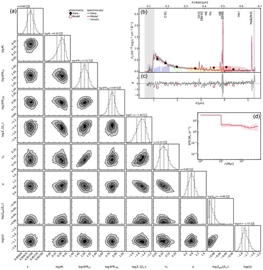
Prospector fitting results of the Main component. (a) Corner plot of the fitted parameters: redshift, stellar mass, SFR averaged over 10 Myr, SFR averaged over 100 MyR, stellar metallicity, optical depth of the diffuse ISM, extra dust attenuation towards birth clouds, gas metallicity, ionization parameter. (b) Data (black) and the best-fitting model (red) for the photometry and spectroscopic data. (c) Visualization of the residuals of the photometric and spectroscopic data. (d) Star-formation history with the red shaded region indicating the 68 per cent confidence interval.
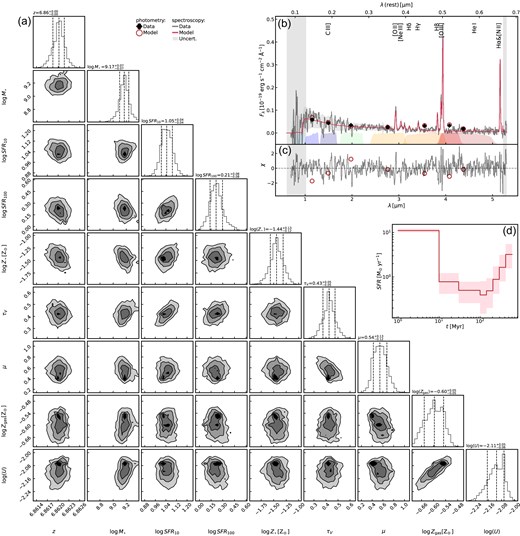
Same as Fig. B1, but for the North component.
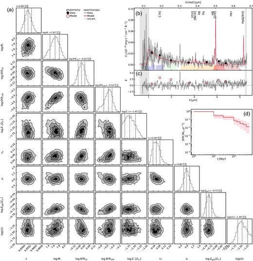
Same as Fig. B1, but for the East component.
