


ABSTRACT
We present the MeerKAT discovery and MeerLICHT contemporaneous optical observations of the fast radio burst (FRB) 20230808F, which was found to have a dispersion measure of |$\mathrm{DM}=653.2\pm 0.4\mathrm{\, pc\, cm^{-3}}$|. FRB 20230808F has a scattering time-scale |$\tau _{s}=3.1\pm 0.1\, \mathrm{ms}$| at 1563.6 MHz, a rotation measure |$\mathrm{RM}=169.4\pm 0.2\, \mathrm{rad\, m^{-2}}$|, and a radio fluence |$F_{\mathrm{radio}}=1.72\pm 0.01\, \mathrm{Jy\, ms}$|. We find no optical counterpart in the time immediately after the FRB, nor in the 3 months after the FRB during which we continued to monitor the field of the FRB. We set an optical upper flux limit in MeerLICHT’s q-band of |$11.7\, \mathrm{\mu Jy}$| for a 60 s exposure which started |${\sim}3.4$| s after the burst, which corresponds to an optical fluence, |$F_{\mathrm{opt}}$|, of |$0.039\, \mathrm{Jy\, ms}$| on a time-scale of |${\sim}3.4$| s. We obtain an estimate for the |$q-$|band luminosity limit of |$vL_{v}\sim 1.3\times 10^{43}\, \mathrm{erg\, s^{-1}}$|. We localize the burst to a close galaxy pair at a redshift of |$z_{\mathrm{spec}}=0.3472\pm 0.0002$|. Our time delay of |${\sim}3.4$| s between the FRB arrival time and the start of our optical exposure is the shortest ever for an as yet non-repeating FRB, and hence the closest to simultaneous optical follow-up that exists for such an FRB.
1 INTRODUCTION
Fast radio bursts (FRBs), first discovered in 2007, are bright, millisecond-duration pulses of radio emission. FRBs have dispersion measures (DMs) that are far greater than the expected DM contribution of the Milky Way (MW) galaxy, meaning that they are of extragalactic origin. The first FRB was found in archival pulsar data from 2001 that made use of Murriyang, the Parkes 64-m radio telescope (Lorimer et al. 2007), with an additional four bursts discovered in 2013, confirming them as a population (Thornton et al. 2013).
FRBs are subdivided into two main groups: repeaters and non-repeaters, although there is ongoing debate as to whether or not these are two fundamentally different populations. Non-repeating FRBs are those that have only been detected once, and out of the more than 7001 FRBs discovered and published to date, most of them fall into this category. Repeating FRBs, on the other hand, are those which have been observed to burst multiple times, and |$\sim$|60 of this type have been published to date (CHIME/FRB Collaboration 2023). The isotropic energies of FRBs span a range from |${\sim}10^{35}$| to |$10^{43}\, \mathrm{erg}$|.
The DMs of known FRBs span from |$87.82\, \mathrm{pc\, cm^{-3}}$| for the repeater FRB 20200120E, localized to a globular cluster in M81 (Bhardwaj et al. 2021; Kirsten et al. 2022), to |$3338\, \mathrm{pc\, cm^{-3}}$|, for FRB 19920913A (Crawford et al. 2022). The most distant localized FRB is FRB 20220610A, which has a redshift of |$z=1.016\pm 0.002$| (Ryder et al. 2023). Recently, however, Connor et al. (2024) published the newly discovered FRB 20230521B, which they report as having a redshift of |$z=1.354$|. This measurement is tentative for the time being, as it is derived from a single line presumed to correspond to |$\mathrm{H\alpha }$|. If confirmed, it would exceed the redshift of FRB 20220610A.
The origin of FRBs remains unknown, although numerous models have been suggested. Some of these models propose that FRBs originate from compact objects, and there are numerous ones which predict that at least some FRBs come from magnetars (e.g. Beloborodov 2017, 2020; Kumar, Lu & Bhattacharya 2017; Metzger, Berger & Margalit 2017; Yang & Zhang 2018). Cataclysmic models were at first suggested as potential explanations for FRBs (e.g. Falcke & Rezzolla 2014), but these were ruled out as an explanation for all FRBs once some were found to repeat (Spitler et al. 2016; see Platts et al. 2019 and Zhang 2023 for a comprehensive review of FRB progenitor models). The detection of a bright radio burst (Bochenek et al. 2020; CHIME/FRB Collaboration 2020) from SGR 1935 + 2154 (Cummings et al. 2014; Lien et al. 2014; Israel et al. 2016), a Galactic magnetar, gave some evidence for the idea that magnetars can cause some FRBs. The radio burst from SGR 1935 + 2154 is sometimes called the first ‘Galactic’ FRB (FRB 20200428), despite being significantly less luminous than FRBs. There are two main classes of models associated with magnetar progenitors: magnetospheric models, in which the emission comes from close to the surface of the neutron star (Katz 2016; Kumar et al. 2017; Wadiasingh & Timokhin 2019; Kumar & Bošnjak 2020; Lyutikov & Popov 2020; Cooper & Wijers 2021), and maser shock models, in which the pulse results from maser emission in magnetized shocks (Beloborodov 2017; Metzger, Margalit & Sironi 2019; Beloborodov 2020).
It remains unclear whether or not non-repeaters and repeaters have different underlying mechanisms, or whether the non-repeaters are simply repeating at much lower rates, and we therefore have not yet observed their repetition. However, there are some differences which have been observed in the burst structures of non-repeaters versus repeater FRBs: repeaters often display what is known as the ‘sad trombone effect’ (CHIME/FRB Collaboration 2019; Hessels et al. 2019; Day et al. 2020; Fonseca et al. 2020), whereby bursts have multiple components that drift downwards in frequency. Non-repeaters, on the other hand, can have bursts with a single component that can be either broad-band or narrow-band, or bursts with multiple components which all peak at the same frequency. Additionally, repeaters tend to be narrower in frequency and wider in time than non-repeaters (Pleunis et al. 2021).
FRBs have not yet been conclusively observed at other wavelengths, and as such, no counterpart of statistical significance has been found, although there have been multiple attempts (e.g. Petroff et al. 2015; Callister, Kanner & Weinstein 2016; Hardy et al. 2017; Zhang & Zhang 2017; Aartsen et al. 2018; Acciari et al. 2018; Eftekhari et al. 2018; Kilpatrick et al. 2021, 2024; Núñez et al. 2021; Niino et al. 2022; Hiramatsu et al. 2023; Pearlman et al. 2025; Trudu et al. 2023; Xing & Yu 2024). A confirmed optical counterpart would help to rule out at least some of the currently suggested models for FRB emission mechanisms. For example, the synchrotron maser model of FRBs predicts a multiwavelength afterglow, while most magnetospheric models do not. The detection of an optical afterglow would provide evidence in favour of the former model. For the burst associated with SGR 1935 + 2154, Margalit et al. (2020) interpreted the X-ray counterpart as the X-ray afterglow of the FRB. However, the non-detections of an optical afterglow for FRB 20200428 (e.g. Bailes et al. 2021) greatly constrain the maser shock model (Cooper et al. 2022). In this work, we present our discovery of the to date non-repeating FRB 20230808F, and our search for an optical counterpart, utilizing almost simultaneous optical-radio observations.
2 RADIO OBSERVATIONS AND DATA REDUCTION
2.1 MeerTRAP pipeline and FRB 20230808F detection
MeerKAT is a radio telescope array consisting of 64 13.5-m dishes, located in the Karoo in South Africa (Jonas & MeerKAT Team 2016). MeerKAT’s detection of FRBs is carried out by the Transient User Supplied Equipment (TUSE) instrument of MeerTRAP (Meer(more) TRAnsients and Pulsars; Sanidas et al. 2017; Bezuidenhout et al. 2022; Jankowski et al. 2022; Rajwade et al. 2022), which conducts searches for single pulses concurrently in both coherent and incoherent beams (IBs). MeerTRAP is a commensal survey with MeerKAT, and observes simultaneously with all MeerKAT Large Survey Projects and some other projects. The coherent beams (CBs) are formed by a beam-forming instrument called the Filterbanking Beamformer User Supplied Equipment (FBFUSE; Barr 2017; Chen et al. 2021), which coherently combines the signals from the dishes of the telescope array. FBFUSE and TUSE together form the MeerTRAP backend, which can form up to 768 CBs that are highly sensitive and have a total field of view (FoV) of |$\sim$|0.4 |$\mathrm{deg^2}$|. This is only a fraction of the primary FoV of MeerKAT, which is |$\sim$|1 |$\mathrm{deg^2}$| at 1284 MHz, although this fraction also depends on the elevation of the source being observed by the telescope (Chen et al. 2021; Rajwade et al. 2022). The IB is formed by summing the signals from all of the available antennas, resulting in a less sensitive beam which samples the entire |$\sim$|1 |$\mathrm{deg^2}$| FoV and which usually has around one-fifth of the sensitivity of the CBs. AstroAccelerate2 (Dimoudi & Armour 2015; Adámek & Armour 2016; Adámek et al. 2017; Adámek & Armour 2018; Dimoudi et al. 2018), a GPU-based single-pulse search pipeline, is used to perform a real-time search for dispersed bursts, by incoherently de-dispersing the data in the DM range 0–5118.4 pc |$\mathrm{cm^{-3}}$| (see Caleb et al. 2020 for further details about the search process).
FRB 20230808F was detected by MeerTRAP at the L band, which is centred on 1284 MHz and has a bandwidth of 856 MHz, on 2023 August 8. The arrival time at the top of the observing band for the FRB was 03:49:15.888 ut and its DM was found to be |$\mathrm{DM}=653.2\pm 0.4$| pc |$\mathrm{cm^{-3}}$|. The time of arrival at infinite frequency for the FRB was calculated using the arrival time at the top of MeerKAT’s L band (1712 MHz) and taking into account the frequency dispersion in the burst arrival time, due to the ionized interstellar and intergalactic medium.3 This resulted in an arrival time at the MeerKAT site of 03:49:14.963 ut on 2023 August 8 at infinite frequency.
2.2 Localization
The detection of FRB 20230808F in a CB and the IB provides an approximate region of the sky from which the burst originated. The burst passed the detection and machine learning criteria within 45 s after the detection, triggering a transient buffer (TB) data dump, whereby high-resolution data around the time of a transient event is captured and stored. The TB data was used to localize the FRB, as well as to obtain the beam-formed data which has a higher spectrotemporal resolution. A detailed description of the MeerTRAP TB system and FRB localization can be found in Rajwade et al. (2024).
The TB data provides a complex voltage data set, which contains all of the voltages received by MeerKAT’s antennas that were active at the time of the burst detection. The voltage data contain 300 ms of signal tracing the dispersion curve of the FRB, which is divided into 64 equal subbands. The data were imaged using WSClean (Offringa et al. 2014), producing a separate image for each frequency subband. Following this, we used Python to produce the images which would be used to search for the FRB. This entailed visually inspecting the full 300-ms images so as to flag and then discard the subbands which contained radio frequency interference (RFI), before the remaining images were averaged to produce an RFI-free image that was used as a reference image to look for the burst. In addition, images with shorter integration times were produced, in order to determine whether any new source appeared during the central milliseconds, which would be the FRB. In the case of FRB 20230808F, the 300 ms were divided into 31 time intervals, and these smaller time-scales were imaged, again averaging the RFI-free frequencies. Difference images were then produced by subtracting the full integration time image from each of the smaller time interval images. A source was found in the difference images for the central time intervals, and, with a location coincident with the CB where it was detected, we concluded that this was the FRB. The full 300 ms were then divided into 489 time intervals in order to enable selection of all images in which the burst was detected, from which we produced an ‘on’ image. Similarly, an ‘off’ image was created containing the same number of time bins, but where the FRB was not present. These on and off images, as well as a new full integration time image, were produced and cleaned with WSClean,4 using the following parameters: the stopping criteria were 100 iterations, or a threshold of 0.01 (arbitrary units). We applied a Cotton-Schwab (Schwab 1984) cleaning with major iteration gain of 0.8, and automasking threshold of |$\sigma =3$|. We used a Briggs weighting with a robustness parameter of |$-0.3$| with a weight rank filter of 3. Lastly, we applied a W-gridding mode. The final images were centred at the phase centre of the observation, they have a pixel size of |$1 \, \text{arcsec}^2$|, and a size of |$4096\times 4096$| pixels. The clean on and off images, zoomed at the location of the FRB, are shown in Fig. 1.

‘Off’ and ‘on’ cleaned images showing the burst of FRB 20230808F. Each image has a total exposure time of approximately 14.7 ms.
Following this, astrometry was performed using the method described in Driessen et al. (2024), by running the Python Blob Detector and Source Finder (pybdsf; Mohan & Rafferty 2015) algorithm to identify the positions of the sources in the images. The astrometric transformation was obtained by searching other radio catalogues with known sources in the FoV, which were used as references. Although we prioritize using catalogues with a positional accuracy <0.5 arcsec, the FoV of FRB 20230808F is not covered by any such catalogues containing sufficient sources to perform the astrometric correction (|${\gtrsim}5$|). While the Rapid ASKAP Continuum Survey (RACS-mid; Duchesne et al. 2023) contains sufficient sources within the FRB FoV, its sources have systematic positional uncertainties of 1–2 arcsec. Thus, as described in Rajwade et al. (2024), we use the Radio Fundamental Catalogue (RFC)5 to correct the RACS-mid source positions. The RFC has source positions with milliarcsecond accuracy, and while it does not contain enough sources to perform the astrometric correction of the FRB FoV, it is enough to correct the RACS-mid source positions within a 5 degree radius. We then used the RACS-mid corrected source positions to correct the MeerKAT images. The astrometric correction was performed with the python package astroalign (Beroiz, Cabral & Sanchez 2020), and only sources classified as point-like were used. The transformation was applied to the on, off, and full integration time images, and the corrected FRB coordinates were then obtained from the transformed on image. The position errors for the FRB were obtained by summing in quadrature the position error from pybdsf, and the astrometric error from the two transformations, which is defined as the mean angular separation between the sources in the reference catalogue and the corrected coordinates of sources in the target catalogue. In our case, the reference and target catalogues for the first astrometric correction were RFC and RACS, respectively, and for the second correction they were RACS and MeerTRAP. FRB 20230808F was localized to a position of |$\mathrm{RA\, (J2000)=03^{h}33^{m}12^{s}.99\pm 0^{s}.03}$| and |$\mathrm{Dec\, (J2000)=-51^{\circ }56^{\prime }07{_{.}^{\prime\prime}} 02}\pm 0{_{.}^{\prime\prime}} 50$|.
2.3 Burst structure and timing analysis
Using the localized FRB coordinates, the TB data were beamformed at the correct FRB position, resulting in a boost in the signal-to-noise ratio (S/N; see Rajwade et al. 2024 for further details of this process). The TB data had a higher spectrotemporal resolution, and were coherently de-dispersed at the DM of the burst, eliminating intra-channel smearing. The beamformed data were used to resolve the FRB components, along with the scattering time-scale. To fit the temporal structure of the FRB, the frequency range where the burst emission was most visible – primarily at the upper end of the observing bandwidth – was selected to enhance the S/N of the pulse profile. This involved averaging the dynamic spectrum in time, fitting it with a Gaussian function, and then selecting frequencies within the Full Width at Tenth Maximum (FWTM) of the fitted Gaussian. For FRB 20230808F, this range spanned from 1415.25 to 1738.23 MHz. The upper frequency limit is above the maximum of MeerKAT’s L-band, so all channels above 1415.25 MHz up to 1712 MHz were included. In order to fit the pulse to a multicomponent model with scattering, a semi-automated fitting routine was created to select the locations of the components, fit multicomponent scattered Gaussians, and then find the optimal number of components and scattering time-scale. The fitting routine models the pulse profile of an FRB using a multicomponent scattered Gaussian model. This is done by first smoothing the pulse profile with a Blackman window of length 15 and identifying local maxima within the smoothed pulse profile. A range for the number of components (minimum and maximum) is provided as input, and the largest peaks in the smoothed profile are used as initial guesses for the component locations. The profile is then fitted iteratively using lmfit.Minimizer and custom functions that convolve multiple Gaussians with a one-sided exponential decay to add scattering. The fitting process minimizes the difference between the model and the data, adding components iteratively by smoothing residuals and identifying additional peaks, until the maximum component number is reached. The optimal number of components is then chosen based on the lowest Bayesian Information Criterion (BIC), yielding the number of components, scattering time-scale, and the arrival time, amplitude, and width of each component. This resulted in an optimal number of components of 6, along with the time of arrival (ToA) of each component, and a scattering time-scale |$\tau _{s}=3.1\pm 0.1$| ms. The latter is measured at 1563.6 MHz, which is the central frequency of the burst bandwidth. The locations of the 6 burst components are shown in Fig. 2.
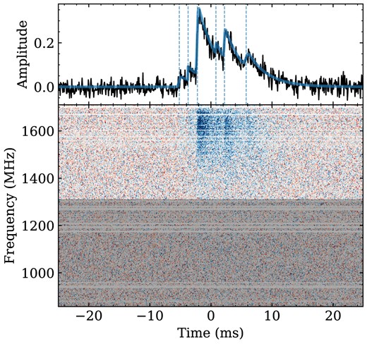
The dynamic spectrum and burst profile of FRB 20230808F. The black solid line in the top panel shows the averaged pulse profile, the solid blue line shows the fit to a multicomponent scattered Gaussian, and the dashed blue lines indicate the positions of the six burst components. The dynamic spectrum is shown in the bottom panel, with the shaded grey area showing the region outside of the FWTM of the spectrum.
The method described in Pastor-Marazuela et al. (2023) was used to test for periodicity in the burst structure and to obtain the component arrangement. The ToAs as a function of component number were fitted to a linear function of the form:
where |$t_{i}$| is the ith arrival time, |$\bar {d}$| is the mean spacing between the subcomponents of the burst, |$n_i$| is the ith component number, and |$T_0$| is the first ToA. The fitting was conducted using the python package lmfit6 (Newville et al. 2024). A least-squares minimization technique, weighted by the inverse of the ToA errors, was used to determine the mean subcomponent separation |$P_\mathrm{{sc}}$|, equivalent to |$\bar {d}$|, and the goodness of fit was assessed using the reduced chi-squared statistic, |$\chi _{r}^2$|. This yielded |$P_\mathrm{{sc}}=1.55\pm 0.03$| ms.
To test the significance of the periodicity, |$10^5$| bursts with six subcomponents and random separations were simulated and the same linear fit described by equation (1) was performed, with the resulting distribution of |$\chi _{r}^2$| values compared to the |$\chi _{r}^2$| for the FRB. The subburst separations were simulated using two different distributions, namely a rectangular and a Poissonian distribution, and using different exclusion parameters. The exclusion parameter |$\eta$| is the minimal separation fraction that we consider would be resolved by the fitting routine. Using rectangular simulations, the periodicity significance was equal to |$2.22\, \mathrm{\sigma }$|, while for the Poissonian distribution, the significance was |$2.11\, \mathrm{\sigma }$|. In both cases, therefore, we do not find that the burst is significantly periodic.
2.4 Polarization and rotation measure
The TB data provide full Stokes I, Q, U, and V information, which was used to obtain the RM and intrinsic polarization properties of the burst. The Faraday RM for FRB 20230808F was measured using the RM-Tools algorithm (Purcell et al. 2020), which applies the RM synthesis technique (Burn 1966; Brentjens & de Bruyn 2005). This yielded a |$\mathrm{RM}=169.4\pm 0.2$| rad |$\mathrm{m}^{-2}$|. We then de-rotated the Stokes Q/U data at the measured RM, which removed any variations with frequency and enabled us to study the intrinsic emission. The average linear polarization factor, L/I, was found to be |$106.6\pm 14.8$| per cent, while the average circular polarization factor, V/I, was found to be |$10.4\pm 7.8$| per cent. These values are consistent with 100 per cent linear and 0 per cent circular polarization fractions, which is what is commonly observed in repeating and some one-off FRBs (e.g. Michilli et al. 2018; Cho et al. 2020; Day et al. 2020; Luo et al. 2020). The polarization position angle (PPA) is given by
The PPA is shown in the top panel of Fig. 3, and we found that it appears to step from |$60^{\circ }$| to |$80^{\circ }$| over the duration of the burst, which is consistent with behaviour seen in multiple pulsars and magnetars, and other FRBs (e.g. Cho et al. 2020; Luo et al. 2020).

The Stokes I, Q, U, and V data for FRB 20230808F are shown in the four bottom panels, prior to the de-rotation of Stokes Q/U. The top two panels show the PPA and pulse profile, respectively, both after de-rotating Q/U, and a scattering tail is visible in the pulse profile. The blue in the Stokes panels indicates positive intensity values, while red is associated with negative values.
3 HOST GALAXY AND OPTICAL COUNTERPART SEARCH
3.1 Identification of host galaxy
After localizing the FRB, we searched at the coordinates of the burst in the Dark Energy Spectroscopic Instrument (DESI; DESI Collaboration 2016) Legacy Survey’s tenth data release (hereafter DESI DR10), and it was apparent that there were two potential host galaxies, although the burst location appeared closer to one of the two. From visual inspection, the two galaxies appeared to possibly be interacting, as can be seen, along with the FRB coordinates, in Fig. 6. The coordinates of the two galaxies are |$\mathrm{RA\, (J2000)=03^{h}33^{m}12^{s}.70,\, Dec\, (J2000)=-51^{\circ }56^{\prime }06{_{.}^{\prime\prime}} 72}$| for the northernmost galaxy (hereafter north galaxy) and |$\mathrm{RA\, (J2000)=03^{h}33^{m}12^{s}.83,\, Dec\, (J2000)=-51^{\circ }56^{\prime }09{_{.}^{\prime\prime}} 27}$| for the southernmost galaxy (hereafter south galaxy).
We run the Probabilistic Association of Transients to their Hosts (PATH) algorithm (Aggarwal et al. 2021) for a sample of galaxies from DESI DR10 within a FoV of 30 arcsec around the FRB position. PATH is a Bayesian algorithm that provides posterior probabilities (|$P(O_i|x)$|) for host associations based on observables and priors that depend only on photometry and astrometry (including the FRB position uncertainty). We used photometry in the r-band with an exponential profile prior centred in each candidate galaxy with a characteristic scale given by their half-light radii (|$r_e$|) up to a maximum of |$10\times r_e$|. We also used a prior on the true host not being included in the catalogue (i.e. ‘unseen’) of |$P(U)=0.05$|. The rest of the parameters were set as default in the PATH repository.7 We obtained |$P(O_i|x)=0.59$| and |$P(O_i|x)=0.37$|, for the north and south galaxy, respectively. Changing the characteristic scale of the prior exponential profile to |$r_e/2$| as suggested by Shannon et al. (2024) does not significantly change the posteriors. This analysis provides support to the association of the FRB with either of the two closest identified galaxies, with the sum of these posterior probabilities being larger than 0.9. We note that, while PATH assigns a higher association probability to the north galaxy, the algorithm does not take into account the ellipticity and orientation of the host galaxy candidates. From the optical image, shown in Fig. 6, the FRB localization seems to fall within the extension of the south galaxy.
Zou et al. (2022) calculated the photometric redshifts for around 293 million galaxies with i < 24 in DES DR2, including the two potential host galaxies. The photometric redshift for the north galaxy from Zou et al. (2022) is |$z_{\mathrm{phot}}=0.42\pm 0.06$|, while that of the south galaxy is |$z_{\mathrm{phot}}=0.53\pm 0.07$|. These two redshifts agree within uncertainties, implying that the galaxies may be a close, potentially interacting pair. The DESI DR10 magnitudes for the galaxies are presented in Table 1, and various properties of the galaxies resulting from the SED fitting are shown in Table 2. The star formation rates (SFRs) obtained for both galaxies are negative, which likely means that the true SFR is low, consistent with zero. We also note the comment made by the authors, which cautions the reader against using the SFR and stellar age parameters from their catalogue.
DESI DR10 magnitudes for the two potential identified host galaxies.
| Filter | North galaxy | South galaxy |
|---|---|---|
| g | 22.3 | 22.9 |
| r | 21.4 | 21.6 |
| i | 21.0 | 21.1 |
| z | 20.6 | 20.7 |
| Filter | North galaxy | South galaxy |
|---|---|---|
| g | 22.3 | 22.9 |
| r | 21.4 | 21.6 |
| i | 21.0 | 21.1 |
| z | 20.6 | 20.7 |
Estimated age, log stellar mass, and SFR for each of the potential host galaxies, obtained from the SED fitting performed by Zou et al. (2022). The upper SFR refers to the upper limit of the SFR with a 68 per cent confidence level.
| Property | North galaxy | South galaxy |
|---|---|---|
| Age (yr) | |$8\times 10^9$| | |$4\times 10^9$| |
| Mass (dex) | 10.26 | 10.33 |
| Best SFR (|$M_{\odot }\, \mathrm{yr^{-1}}$|) | |$-0.1$| | |$-0.1$| |
| Upper SFR (|$M_{\odot }\, \mathrm{yr^{-1}}$|) | 0.2 | 0.0 |
| Property | North galaxy | South galaxy |
|---|---|---|
| Age (yr) | |$8\times 10^9$| | |$4\times 10^9$| |
| Mass (dex) | 10.26 | 10.33 |
| Best SFR (|$M_{\odot }\, \mathrm{yr^{-1}}$|) | |$-0.1$| | |$-0.1$| |
| Upper SFR (|$M_{\odot }\, \mathrm{yr^{-1}}$|) | 0.2 | 0.0 |
3.2 MeerLICHT optical counterpart search
MeerLICHT, situated at the South African Astronomical Observatory site near Sutherland in South Africa, is a fully robotic, wide-field optical telescope. The telescope has a 0.65 m primary mirror and a 2.7 |$\mathrm{deg^2}$| FoV, and was built as a prototype for the BlackGEM array in Chile (Groot et al. 2024). MeerLICHT has a filter wheel that consists of the Sloan Digital Sky Survey (York et al. 2000) u, g, r, i, and z filters, and a wider q band that spans the range of 440–720 nm (Groot et al. 2024). MeerLICHT has a declination upper limit of |$+30^{\circ }$|, and pointing limits of |$\gt 20^{\circ}$| above the horizon in elevation and hour angle limit greater than |$-3$| h and less than 4.5 h. When the aforementioned conditions are met, MeerLICHT co-observes with MeerKAT, and if syncing cannot be established for one or more reasons, the telescope either follows its backup programme of observing regions of Local Universe mass overdensities, follows up other high-priority targets, or it builds up reference images for its survey of the southern sky.
When MeerLICHT is synced with MeerKAT, it observes in 1-min exposures, and every second image is a q-band exposure in the sequence q, g, q, i, q, u, q, r, q, z, q. When not synced with MeerKAT, MeerLICHT observes in the filter sequence q, u, i, q, u, i, etc., also with an integration time of 1 min. Regardless of whether or not it is linked with MeerKAT, there are approximately 25 s of overhead time in between each MeerLICHT exposure, which allows for filter change, re-pointing of the telescope, and image readout.
MeerLICHT images are reduced using two pieces of python software: BlackBOX (Vreeswijk & Paterson 2021a) and ZOGY8 (Zackay, Ofek & Gal-Yam 2016; Vreeswijk & Paterson 2021b). Routine CCD reduction procedures are carried out by BlackBOX on the raw science images, and then ZOGY performs source identification, photometry, astrometry, and finds transient candidates. The method for finding transient candidates is based on the image subtraction routine developed by Zackay et al. (2016). The reduced images are available on ilifu, which is a cloud facility9 operated by the Inter-University Institute for Data Intensive Astronomy (IDIA) and hosted at the University of Cape Town.
One of MeerLICHT’s primary science goals is to try and simultaneously observe FRBs, along with MeerKAT/MeerTRAP. In the early morning on 2023 August 8, MeerLICHT synced with MeerKAT while the latter was observing the MHONGOOSE (SCI-20180516-EB-01) field where the FRB occurred, which corresponds to the MeerLICHT fixed sky-grid field 16074. MeerLICHT commenced observations of the field at around 02:05 ut. The arrival time of FRB 20230808F occurred while the two telescopes were linked, although it was within MeerLICHT’s overhead time, in between a u-band exposure and a q-band exposure. The q-band exposure started approximately 3.4 s after the arrival time of the FRB, at 03:49:18.32 ut.
The MeerLICHT exposures taken of field 16 074 were accessed using ilifu, where we first visually inspected the images taken immediately before and after the arrival of the FRB. No obvious optical emission at the location of the FRB was seen. We created co-adds around the time of the FRB as well, using the co-adding package for MeerLICHT, buildref.py.10 The following co-adds were made: a co-add per filter of all MeerLICHT images of field 16074 until 5 d before the FRB (hereafter referred to as the deep co-add), a co-add per filter of all exposures of the field in the 20 min before the FRB, one per filter of all exposures in the 20 min after the FRB, and then 15 min before and after, 5 min before and after, and 1 min before and after the burst arrival time. As the MeerLICHT exposures are 60 s in length, the ‘1-min’ co-adds each had one image only. We then ran ZOGY to perform image subtraction, using the deep co-add for each filter as a reference image, and subtracting these from all of the other co-adds. After performing the image subtraction, we ran the forced photometry package for MeerLICHT, force_phot.py11 (Vreeswijk et al. in preparation), on the resulting images in order to extract flux measurements at the coordinates of the FRB at various times around the arrival of the burst. Photometric and astrometric calibrations for MeerLICHT data are carried out using a catalogue of Gaia DR2 (Brown et al. 2018) stars.
MeerLICHT re-observed field 16 074 on the night of 2023 September 6. We chose a 300 s integration time, as opposed to the usual 60 s, so that we could obtain deeper exposures of the field. These images – five each in the u, q, i, and z bands and four in the g band – were then also co-added and we ran image subtraction and forced photometry on the resulting co-added images. In addition, field 16074 was given high priority status in MeerLICHT’s scheduler, so that it would be observed more frequently as part of MeerLICHT’s backup programme whenever it was not synced with MeerKAT. As a result of this, the field was observed regularly over the subsequent months, and we created a co-add per filter of all of the MeerLICHT exposures of the field in the 3 months post-FRB, as well as ‘per night’ co-adds for all of the individual nights post-FRB on which the field was observed.
We corrected for MW dust extinction for all of our photometry results. We found the colour excess in the MW in the direction of FRB 20230808F, |$E(B-V)_{\mathrm{MW}}$|, in each of MeerLICHT’s filters, based on the colour excess map by Schlafly & Finkbeiner (2011).12 We assumed the Fitzpatrick (1999) reddening law with |$R_{V}=3.1$|, where |$R_{V}$| is the total-to-selective extinction ratio. The MW-dust-extinction-corrected photometry results can be seen in Table 3, and are also shown in Figs 4(a) and (b).

Forced photometry results for FRB 20230808F. In both plots, each colour represents a different MeerLICHT filter, upside down triangles indicate limiting magnitudes, and stars represent actual magnitude measurements where the S/N was greater than 3. The dashed black line in each plot indicates the MJD at which FRB 20230808F took place. The forced photometry results from the night of the FRB, with apparent magnitude plotted against modified Julian date (MJD), and horizontal errorbars representing the time-span over which a co-add was made, are shown in (a). The forced photometry results at the FRB coordinates, for all of the MeerLICHT images of field 16074, but excluding the deep co-add, are shown in (b). The deep co-add is excluded because it was used as the reference image for image subtraction. For upper limits obtained from co-added images spanning a short time range, the horizontal error bars are not visible in (b).
Upper limits on optical emission for FRB 20230808F, corrected for MW dust extinction.
| Filter | Upper limit or detection magnitude (AB) | Upper limit or detection flux (|$\mathrm{\mu Jy}$|) | Filter | Upper limit or detection magnitude (AB) | Upper limit or detection flux (|$\mathrm{\mu Jy}$|) |
|---|---|---|---|---|---|
| 1 min before | 1 min after | ||||
| u | 19.7 | 46.9 | q | 21.2 | 11.7 |
| 5 min before | 5 min after | ||||
| u | 19.7 | 46.9 | q | 21.6 | 8.2 |
| q | 21.7 | 7.5 | r | 20.6 | 20.0 |
| i | 20.3 | 28.5 | z | 19.2 | 74.7 |
| 15 min before | 15 min after | ||||
| u | 19.7 | 46.9 | u | 19.5 | 57.0 |
| g | 20.9 | 16.5 | g | 20.7 | 19.4 |
| q | 22.2 | 4.7 | q | 22.0 | 5.7 |
| r | 20.7 | 19.1 | r | 20.6 | 20.0 |
| i | 20.3 | 28.5 | i | 20.0 | 36.4 |
| z | 19.3 | 68.8 | z | 19.2 | 74.7 |
| 20 min before | 20 min after | ||||
| u | 20.1 | 32.9 | u | 19.5 | 57.0 |
| g | 20.9 | 16.5 | g | 20.7 | 19.4 |
| q | 22.4 | 4.0 | q | 22.1 | 5.2 |
| r | 20.7 | 19.1 | r | 20.9 | 15.3 |
| i | 20.6 | 20.0 | i | 20.0 | 36.4 |
| z | 19.3 | 68.8 | z | 19.2 | 74.7 |
| 2023-08-01 | 2023-08-02 | ||||
| u | 20.4 | 26.1 | u | 19.8 | 42.2 |
| g | 21.2 | 12.1 | g | 20.7 | 18.4 |
| q | 22.5 | 3.7 | q | 22.1 | 5.4 |
| r | 21.2 | 12.0 | r | 20.8 | 17.3 |
| i | 21.1 | 13.1 | i | 20.5 | 22.1 |
| z | 20.3 | 28.5 | z | 19.6 | 50.2 |
| 2023-09-06 | 2023-10-01 | ||||
| u | 22.0 | 6.0 | u | 19.0 | 95.5 |
| g | 22.5 | 3.7 | q | 20.5 | 22.5 |
| q | |$22.3\pm 0.2$| | |$4.3\pm 0.6$| | i | 19.9 | 39.9 |
| i | |$21.7\pm 0.2$| | |$7.5\pm 1.6$| | |||
| z | 21.3 | 10.7 | |||
| 2023-10-02 | 2023-10-03 | ||||
| u | 19.1 | 85.9 | u | 19.5 | 57.5 |
| q | 20.6 | 20.1 | q | 21.4 | 10.1 |
| i | 19.8 | 44.7 | i | 20.1 | 32.0 |
| 2023-10-04 | 2023-10-17 | ||||
| u | 18.5 | 151.0 | u | 20.6 | 21.8 |
| q | 20.4 | 24.7 | q | |$22.2\pm 0.3$| | |$4.7\pm 1.3$| |
| i | 19.1 | 85.8 | i | 21.2 | 12.4 |
| 2023-10-18 | 2023-10-19 | ||||
| u | 20.0 | 37.4 | u | 21.9 | 6.0 |
| q | 21.8 | 6.9 | q | |$22.3\pm 0.1$| | |$4.3\pm 0.6$| |
| i | 20.2 | 29.7 | i | |$21.8\pm 0.3$| | |$6.7\pm 1.6$| |
| 2023-10-25 | 2023-10-26 | ||||
| u | 21.1 | 13.8 | u | 20.1 | 33.3 |
| q | 22.5 | 3.8 | q | 21.5 | 8.9 |
| i | 21.6 | 8.5 | i | 20.8 | 17.7 |
| 2023-10-29 | 2023-10-30 | ||||
| q | 20.0 | 37.0 | u | 20.0 | 37.5 |
| q | 21.3 | 10.7 | |||
| i | 20.6 | 21.0 | |||
| 2023-10-31 | 2023-11-01 | ||||
| u | 20.0 | 37.1 | u | 19.3 | 71.2 |
| q | 21.4 | 9.7 | q | 21.4 | 9.9 |
| i | 19.8 | 44.7 | |||
| 2023-11-02 | 2023-11-04 | ||||
| u | 19.2 | 78.1 | u | 21.0 | 14.0 |
| q | 21.0 | 14.7 | q | |$22.3\pm 0.2$| | |$4.2\pm 0.9$| |
| i | 19.5 | 59.4 | i | 21.5 | 8.9 |
| 2023-11-07 | 3 months post-FRB | ||||
| u | 20.7 | 19.9 | u | 22.3 | 4.3 |
| q | |$21.9\pm 0.2$| | |$6.5\pm 1.3$| | g | 22.4 | 3.8 |
| i | 21.0 | 14.5 | q | |$23.8\pm 0.1$| | |$1.1\pm 0.1$| |
| r | 20.9 | 15.3 | |||
| i | |$22.0\pm 0.2$| | |$5.7\pm 1.1$| | |||
| z | 21.3 | 10.7 | |||
Our deep co-add, shown in Fig. 5, shows a faint underlying extended source at the coordinates of the FRB. This is consistent with the north and south galaxies identified in Section 3.1.
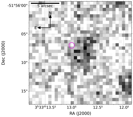
Co-add image produced using all MeerLICHT data of the field of FRB 20230808F up until shortly before the burst. The magenta ellipse indicates the position of the FRB, and the underlying galaxies are visible but unresolved in this image. The resolved galaxies are shown in Fig. 6.
3.3 Southern African Large Telescope spectra
We observed the two galaxies using the Robert Stobie Spectrograph (Burgh et al. 2003) on the 11 m Southern African Large Telescope (SALT; Buckley, Swart & Meiring 2006), to determine their spectroscopic redshifts.
We observed the field of FRB 20230808F on four separate occasions, and the summary of the observations is shown in Table 4.
Observation parameters for the four SALT observations.
| Date | No. exposures | Length of each exposure (s) |
|---|---|---|
| 2023 November 3 | 2 | 1200 |
| 2023 November 5 | 2 | 1200 |
| 2023 December 11 | 2 | 1800 |
| 2023 December 16 | 2 | 1700 |
| Date | No. exposures | Length of each exposure (s) |
|---|---|---|
| 2023 November 3 | 2 | 1200 |
| 2023 November 5 | 2 | 1200 |
| 2023 December 11 | 2 | 1800 |
| 2023 December 16 | 2 | 1700 |
For our two observations in November, the SALT Imaging Camera (SALTICAM), SALT’s sensitive acquisition camera, had been removed for repairs, and a backup CCD camera, BCAM, was in its place. BCAM is a basic Apogee CCD camera, and is much less sensitive than SALTICAM. The position angle (PA) of the slit was set to |$-40^{\circ }$|, and we used a slit width of |$1.5^{\prime \prime }$|. We had initially requested a slit PA of |$-25^{\circ }$|, to pass through both galaxy nuclei as well as two faint alignment stars, but the alignment stars were too faint for BCAM, and as such, we had to adjust the PA to allow for a much brighter alignment star. SALT took these two observations using the PG0700 grating, which covers a wavelength range of 320–900 nm. The obtained spectra were faint in the continuum, but with a clear emission line at 5021 Å.
For the observations on 2023 December 11, the same spectral set-up as before was used, but this time with SALTICAM, and therefore the originally desired slit PA of |$-25^{\circ }$| was used. The final observations on the 2023 December 16 again used SALTICAM, but this time with a redder spectral set-up, using a slit width of |$1.25^{\prime \prime }$| and the PG0900 grating, which also spans 320–900 nm but has higher usable angles, increasing the spectral resolution and efficiency at longer wavelengths. A possible emission line was observed at 8840 Å, although the spectrum was heavily impacted by skyline residuals. The slit orientations for all of the SALT observations are shown in Fig. 6.

The two host galaxy candidates can be seen in the i-band image above, taken from the Dark Energy Survey’s (DES; The Dark Energy Survey Collaboration 2005) second public data release (hereafter DR2; Abbott et al. 2021). The magenta ellipse indicates the position with uncertainties of FRB 20230808F. The black parallel lines indicate the slit position for the November SALT observations, and the blue and red parallel lines show the slit for the 2023 December 11 and 2023 December 16 observations, respectively.
The emission line at 5021 Å was determined to be the [O ii] doublet, which corresponds to a redshift of |$z_{\mathrm{spec}}\sim$|0.347, and there are confirming H |$\beta$| and [O iii] lines at the same redshift at 6548 Å and 6743 Å, respectively. All three lines are clearly visible in the exposures from 2023 November 5 and 2023 December 11, while the spectrum from 2023 November 3 shows the [O ii] and H |$\beta$| emission lines. The emission line at 8840 Å from 2023 December 16 matches the expected position of H |$\alpha$| at the calculated redshift. The spectra from all four nights are shown, with their identified emission lines labelled in the rest frame, in Figs 8(a)–(d). The emission in all of the spectra was determined to be from the north galaxy by comparing the distances between the traces in the 2D spectra and the distances between the reference stars and the galaxies in the various observation set-ups. An example of this is shown in Fig. 7.

2D trace from a SALT observation on 2023 December 11, with the DES DR2 image of the host galaxies positioned alongside to the left. The two reference stars used on that night are aligned with their respective traces, and two yellow line segments are aligned with the centre of the faint trace, from which we obtained the spectrum. The left line segment passes through the north galaxy, indicating that the spectrum obtained is associated with the north galaxy.
![SALT spectra obtained over the course of four nights in late 2023. (a) Shows the average combined spectrum from the two observations on 2023 November 3. The unresolved [O ii] doublet and H$\beta$ lines are shown by the red lines at 3727 Å and 4862 Å, respectively. (b) Shows the average combined spectrum from the two observations on 2023 November 5. The [O ii], H $\beta$ and [O iii] lines are all shown in red, at 3727 Å, 4862 Å, and 5008 Å, respectively. (c) Shows the average combined spectrum from the two observations on 2023 December 11. The [O ii], H $\beta$, and [O iii] lines are all shown in red, at 3727 Å, 4862 Å, and 5008 Å, respectively. (d) Shows the average combined spectrum from the two observations on 2023 December 16. The H $\alpha$ emission line is indicated by a red line and the wavelength ranges that have been affected by sky lines are highlighted in grey.](https://oup.silverchair-cdn.com/oup/backfile/Content_public/Journal/mnras/538/3/10.1093_mnras_staf289/1/m_staf289fig8.jpeg?Expires=1750190218&Signature=cmfudoK6egqyRXjFSyBdt1B7TWr2LkpYAzYDrMrF1AMhReNj9rNfRdza0ZVd1kwiAmMHKgQdW1fzZkbweoX5Ikjykdr0lsoNFVnyFZB3-H067hXID9Zf3nS7LgQHdHOKOVrT0OFiQNpdDgF4X4fMcfaV05dQ4Z73ThM~gZrfMLi9VLnJV1HHvc-gmSmc2X50OPj5K-ptvGOKNICAPflnjyZJtSFclUq1~-tnTDJ6ro-hSr3~ojpcgDEap5TlWuSswrI7pTUbBdhLmCyIs~MtC5oRtpP9-bqCOnSRbJSaQvPd6tYJ~6IBqy1TwH~pfRcv195H51KLi50Uv-hTmbY18A__&Key-Pair-Id=APKAIE5G5CRDK6RD3PGA)
SALT spectra obtained over the course of four nights in late 2023. (a) Shows the average combined spectrum from the two observations on 2023 November 3. The unresolved [O ii] doublet and H|$\beta$| lines are shown by the red lines at 3727 Å and 4862 Å, respectively. (b) Shows the average combined spectrum from the two observations on 2023 November 5. The [O ii], H |$\beta$| and [O iii] lines are all shown in red, at 3727 Å, 4862 Å, and 5008 Å, respectively. (c) Shows the average combined spectrum from the two observations on 2023 December 11. The [O ii], H |$\beta$|, and [O iii] lines are all shown in red, at 3727 Å, 4862 Å, and 5008 Å, respectively. (d) Shows the average combined spectrum from the two observations on 2023 December 16. The H |$\alpha$| emission line is indicated by a red line and the wavelength ranges that have been affected by sky lines are highlighted in grey.
The calculated spectroscopic redshift of |$z_{\mathrm{spec}}=0.3472\pm 0.0002$| is in agreement with the photometric redshift of the north galaxy within |$1.13\, \mathrm{\sigma }$|. Using the spectroscopic redshift, we calculated the luminosity distance, |$D_L$|, as |$1903.4\, \mathrm{Mpc}$|, assuming cosmological parameters from the Planck Collaboration VI (2020).
4 FRB 20230808F CHARACTERISTICS
4.1 Radio flux and fluence
The peak flux density for FRB 20230808F was calculated as described in Jankowski et al. (2023), using a modified version of the single-pulse radiometer equation (Dewey et al. 1985):
where |$S_{\mathrm{peak}}$| is the peak flux density, |$\vec{a}$| is the parameter vector, |$\beta$| is the digitization loss factor, which is 1.0 for 8-bit digitization (Kouwenhoven & Voûte 2001), |$\eta _{\mathrm{b}}$| is the beam-forming efficiency, taken to be |$\sim$|1 (Chen et al. 2021), G is the telescope forward gain, |$b_{\mathrm{eff}}$| is the effective bandwidth, |$N_{\mathrm{p}}=2$| is the number of polarizations summed, |$W_{\mathrm{eq}}$| is the observed equivalent boxcar pulse width, |$T_{\mathrm{sys}}=19\, \mathrm{K}$| and |$T_{\mathrm{sky}}$| are the system and sky temperatures, and |$a_{\mathrm{CB}}=0.9$| and |$a_{\mathrm{IB}}=0.8$| are the attenuation factors of the detection CB and the IB. The radio flux density was thus found to be |$S_{\mathrm{peak}}=(157\pm 14)$| mJy, calculated from the filterbank data where the FRB was detected. The fluence |$F_{\mathrm{radio}}$| was then calculated from |$F_{\mathrm{radio}}=S_{\mathrm{peak}}W_{\mathrm{eq}}$|, yielding |$F_{\mathrm{radio}}=(1.72\pm 0.01)\, \mathrm{Jy\, ms}$|.
Using the peak flux density and fluence, we computed the isotropic luminosity, |$L_{p}$|, and energy, E, of the burst, as described in Zhang (2018), using
where |$S_{\nu ,p}$| is the specific peak flux density, |$F_{\nu }$| is the specific fluence, |$\nu _c$| is the central frequency of the observing band, and |$D_L$| is the luminosity distance, obtained in Section 3.3. Using the values pertaining to FRB 20230808F, we obtained |$L_{p}=8.7\times 10^{41}\, \mathrm{erg\, s^{-1}}$| and |$E=7.1\times 10^{39}\, \mathrm{erg}$|. However, we note that using the central frequency when calculating the luminosity and energy would imply a flat burst spectrum, and as such, following the prescription of Aggarwal (2021), we also used the burst bandwidth, instead of the central observing frequency, to calculate the energy and luminosity of FRB 20230808. Doing so yielded |$L_{p}=2.0\times 10^{41}\, \mathrm{erg\, s^{-1}}$| and |$E=1.6\times 10^{39}\, \mathrm{erg}$|.
4.2 Host galaxy contribution to propagation properties
We used the FRBs13 library (Prochaska & Zheng 2019; Prochaska et al. 2023) to calculate the expected DM contributions, RM, and redshift for FRB 20230808.
The total observed FRB DM is the sum of the DM contributions from the MW, MW halo, the intergalactic medium (IGM), and the host galaxy, and can thus be expressed as
The expected MW DM contribution in the direction of the FRB, according to the YMW16 model (Yao, Manchester & Wang 2017), is |$\sim$||$35\, \mathrm{pc\, cm^{-3}}$|, with an expected |$\tau _{s}\sim 4.8\times 10^{-8}$| s in the L band. According to the NE2001 model (Cordes & Lazio 2004), the MW DM contribution is |$\sim$||$27\, \mathrm{pc\, cm^{-3}}$|, with an expected |$\tau _{s}\sim 4.3\times 10^{-8}$| s in the L band. Taking the average between the YMW16 and NE2001 |$\mathrm{DM_{MW}}$| values, we obtain |$\mathrm{DM_{MW}\sim 31\, pc\, cm^{-3}}$|. We used the model from Yamasaki & Totani (2020) to estimate the DM contribution from the MW halo (|$\mathrm{DM_{halo}}$|), which was found to be |$\sim$||$33\, \mathrm{pc\, cm^{-3}}$|.
The redshift upper limit was computed using the cosmological parameters from the Planck Collaboration VI (2020). By applying the Macquart relation (Macquart et al. 2020), we adjusted the value of |$\mathrm{DM_{host}}$| until the predicted redshift matched the spectroscopic redshift of |$0.3472\pm 0.0002$|, thus obtaining |$\mathrm{DM_{host}\sim 420\, pc\, cm^{-3}}$| in the host galaxy reference frame. Subtracting all of the calculated DM contributions from the total observed DM of |$\sim$||$653\, \mathrm{pc\, cm^{-3}}$|, we obtain |$\mathrm{DM_{IGM}\sim 277\, pc\, cm^{-3}}$|.
We calculated the MW contribution to the RM using the Faraday sky model from Hutschenreuter et al. (2022). The expected MW contribution to the RM in the direction of the FRB is |$\sim$||$18\, \mathrm{rad\, m^{-2}}$|, while that at the host was found to be |$\sim$||$274\, \mathrm{rad\, m^{-2}}$|.
The expected MW scattering time-scales are orders of magnitude smaller than the actual FRB scattering time-scale of |$\tau _s = (3.10\pm 0.13)\, \mathrm{ms}$|. The expected scattering time-scales and the calculated values for the DM and RM contributions, indicate that there are significant extragalactic contributions to all of these propagation properties from either the FRB environment, the host galaxy, or a foreground galaxy. However, disentangling the individual contributions from each of these components is challenging.
4.3 Optical flux limits
Table 3 summarizes the upper limits for optical emission in the seconds, minutes and months following the FRB arrival time. For many of the co-adds we created, the S/N was lower than 3, and for these cases we used the limiting magnitude at a significance level of |$3\sigma$| at the coordinates of the FRB instead of the magnitude value and associated error. As such, in Table 3, the limits which include uncertainties are those where the S/N was greater than 3, and hence where the actual magnitude value was used. In such cases, we assume that the measurement is of the underlying host galaxy. Figs 4(a) and (b) show plots of the upper limits derived from the photometry. Points on these plots which have vertical errorbars are those for which actual magnitude measurements were used, whereas points without represent limiting magnitudes. The horizontal ‘error bars’ represent the timespans over which the images used to create the co-adds were obtained.
No optical counterpart was found for FRB 20230808F in our almost simultaneous or follow-up observations. In the time just after the burst, we were able to set an optical upper flux limit in the q-band of |$f_{\mathrm{AB,}q}\lt 11.7\, \mu \mathrm{Jy}$|, while for our u-band observation which ended approximately 24.7 s before the FRB arrival time, we obtained an upper limit of |$f_{\mathrm{AB,}u}\lt 46.9\, \mu \mathrm{Jy}$| We also obtained upper limits on various nights over the course of the 3 months after the FRB.
4.4 Fluence ratio limit and optical luminosity limit
The flux upper limit in the q-band of |$f_{\mathrm{AB,}q}\lt 11.7\, \mu \mathrm{Jy}$| corresponds to a fluence of |$F_{\mathrm{opt}}=0.039\, \mathrm{Jy\, ms}$| if we conservatively assume that the duration of a possible optical burst |$t_{\mathrm{opt}}\approx \Delta t$|, where |$\Delta t\approx 3.4\, \mathrm{s}$| is the time delay between the FRB and the start of our optical observation. Choosing this time-scale allows us to consider the shortest possible optical burst that could still be detectable under our observing conditions, and this is the same time-scale used by Hiramatsu et al. (2023) for calculating fluence limits where there was a delay between the burst arrival time and the start of an optical exposure. We thus obtain a fluence ratio |$F_{\mathrm{opt}}/F_{\mathrm{radio}}\lesssim 0.023$| on a time-scale of |$\sim$||$3.4\, \mathrm{s}$|. We also evaluated the fluence limit on a longer time-scale of the delay time plus the full integration time. In this case, the fluence limit is |$F_{\mathrm{opt}}=0.74\, \mathrm{Jy\, ms}$|, and the fluence ratio is then |$F_{\mathrm{opt}}/F_{\mathrm{radio}}\lesssim 0.43$| on a time-scale of |$\sim$||$63.4\, \mathrm{s}$|.
For our first observation after the FRB, we were able to obtain a MeerLICHT q-band luminosity limit of |$\nu L_{\nu }\sim 1.3\times 10^{43}\, \mathrm{erg\, s^{-1}}$| with a 60 s exposure starting |$\sim$|3.4 s after the arrival of the FRB. This corresponds to an optical energy limit |$E_{\mathrm{opt}}\sim 7.9\times 10^{44}$| erg, which yields an energy ratio |$E_{\mathrm{opt}}/E_{\mathrm{radio}}\lesssim 4.8\times 10^{5}$| if we use the radio burst energy calculated using the burst bandwidth.
5 FRB 20230808F IN CONTEXT
5.1 Comparison to previous optical limits
Hardy et al. (2017) simultaneously observed the repeater FRB 20121102, which has a redshift of |$z=0.19$| (Tendulkar et al. 2017), with the 100-m Effelsberg Radio Telescope and ULTRASPEC, which is mounted on the 2.4-m Thai National Telescope (Dhillon et al. 2014). They detected 13 bursts in the radio and stacked the optical data around the arrival time of each of the bursts. They obtained an optical fluence limit of |$0.17\, \mathrm{Jy\, ms}$| on a time-scale of 141.4 ms, corrected for MW dust extinction, which corresponds to an optical-to-radio fluence ratio limit of |$F_{\mathrm{opt}}/F_{\mathrm{radio}}\lesssim 0.28$|.
The MAGIC Collaboration (2018) conducted simultaneous radio, optical, and very-high-energy (VHE) gamma-ray observations of FRB 20121102, making use of the Arecibo radio telescope and the Major Atmospheric Gamma Imaging Cherenkov (MAGIC) telescope, located on La Palma in the Canary Islands. The MAGIC telescopes are primarily designed for VHE gamma-ray detection, but can also perform optical observations using the central pixel, allowing for simultaneous optical and gamma-ray measurements during their operations. The authors detected five radio bursts and stacked the optical data around the arrival times of the bursts, obtaining optical fluence limits of |$0.025\, \mathrm{Jy\, ms}$| on a time-scale of |$0.1\, \mathrm{ms}$|, |$0.086\, \mathrm{Jy\, ms}$| on a time-scale of |$1\, \mathrm{ms}$|, |$0.25\, \mathrm{Jy\, ms}$| on a time-scale of |$5\, \mathrm{ms}$|, and |$0.36\, \mathrm{Jy\, ms}$| on a time-scale of |$10\, \mathrm{ms}$|. All of these limits were corrected for MW dust extinction and correspond to optical-to-radio fluence ratio limits of |$F_{\mathrm{opt}}/F_{\mathrm{radio}}\lesssim 0.013-0.18$|.
Niino et al. (2022) used Tomo-e Gozen (Sako et al. 2018), a high-speed camera mounted on the Kiso 105-cm Schmidt telescope, located at Kiso Observatory in Japan, to conduct optical observations of the repeater FRB 20190520B, which has a redshift of |$z = 0.24$| (Niu et al. 2022), while simultaneously obtaining radio observations with the Five-hundred-meter Aperture Spherical radio Telescope (FAST). While they detected 11 radio bursts, no corresponding optical emission was found. They obtained MW-dust-extinction-corrected optical fluence limits as deep as |$0.068\, \mathrm{Jy\, ms}$| on a time-scale of 40.9 ms for the individual bursts. A limit of |$0.029\, \mathrm{Jy\, ms}$| was obtained by averaging the optical flux of the 11 bursts. They also investigated the optical fluence on longer time-scales, obtaining a fluence limit of |$0.13\, \mathrm{Jy\, ms}$| on a time-scale of 0.45 s, and |$0.34\, \mathrm{Jy\, ms}$| on a time-scale of 2.1 s. Their limits correspond to |$F_{\mathrm{opt}}/F_{\mathrm{radio}}\lesssim 0.23-2.1$| for individual bursts, and |$F_{\mathrm{opt}}/F_{\mathrm{radio}}\lesssim 0.20$| for the stacked optical limit.
Hiramatsu et al. (2023) conducted simultaneous, follow-up, and serendipitous archival survey observations of 15 well-localized FRBs, consisting of 7 repeating FRBs, 7 non-repeaters, and SGR 1935 + 2154. Their almost simultaneous observation with a 15 s integration time of the repeater FRB 20220912A, which has a redshift of |$z=0.077$| (Ravi et al. 2023) using Binospec (Fabricant et al. 2019) on the 6.5 m MMT Observatory in Arizona, USA, set a limit on the fluence ratio of |$F_{\mathrm{opt}}/F_{\mathrm{radio}}\lesssim 0.00010$| on a time-scale of|$\sim$| 0.4 s. They also observed the FRB using KeplerCam (Szentgyorgyi et al. 2005) on the 1.2 m Telescope at the Fred Lawrence Whipple Observatory in Arizona, USA, and the Sinistro camera on the 1 m telescope at the McDonald Observatory in Texas, USA, in the Las Cumbres Observatory (LCO; Brown et al. 2013a) network. They obtained a luminosity limit |$\nu L_{\nu }\sim 2\times 10^{41}\, \mathrm{erg\, s^{-1}}$| for their Binospec observation, while the luminosity limits for the same FRB that they obtain from simultaneous observations using KeplerCam and LCO range from |${\sim}(0.3-2.9)\times 10^{42}\, \mathrm{erg\, \mathrm{s^{-1}}}$|, which they report as being the deepest luminosity limits to date for an extragalactic FRB. These simultaneous luminosity limits correspond to fluence ratio limits as deep as |$F_{\mathrm{opt}}/F_{\mathrm{radio}}\lesssim 0.0010$|.
Kilpatrick et al. (2024) used the ‘Alopeke high-cadence camera (Scott 2018; Scott et al. 2021) on the Gemini North telescope, located on Mauna Kea in Hawaii, to obtain optical observations of two bursts from the repeater FRB 20180916B, which is at a redshift of |$z=0.034$| (Marcote et al. 2020). These observations occurred simultaneously with radio observations conducted by CHIME. They obtained MW-dust-extinction-corrected optical fluence limits on time-scales of |$\sim$|10.4 ms for each burst, corresponding to optical-to-radio fluence ratio limits of |$F_{\mathrm{opt}}/F_{\mathrm{radio}}\lt 0.002{-}0.007$|.
Trudu et al. (2023) conducted a multiwavelength radio, optical and X/|$\gamma$|-ray campaign on FRB 20180916B. They observed the FRB over the course of 8 months, using the Sardinia Radio Telescope (SRT) and the upgraded Giant Metrewave Radio Telescope (uGMRT; Gupta et al. 2017) for their radio observations. For their optical observations, they made use of the Aqueye + fast photon counter (Barbieri et al. 2009; Zampieri et al. 2015), mounted on the Copernicus telescope, and the IFI + Iqueye fast photon counter (Naletto et al. 2009), mounted on the Galileo telescope, both located in Asiago. Additionally, they made use of the Calar Alto 2.2 m telescope, the 2.5 m telescope at the Caucasian Mountain Observatory (CMO) of the Sternberg Astronomical Institute (SAI) Lomonosov Moscow State University (MSU), and the SiFAP2 fast photometer (Ghedina et al. 2018; Ambrosino et al. 2016) on the 3.6 m Telescopio Nazionale Galileo (TNG) in the Canary Islands. The deepest simultaneous optical fluence upper limits they obtained with Aqueye + were |$0.005\, \mathrm{Jy\, ms}$| on a time-scale of 200 ms, and |$0.009\, \mathrm{Jy\, ms}$| on a time-scale of 30 s in November 2020. In August 2021, they obtained upper limits of |$0.005\, \mathrm{Jy\, ms}$| on a time-scale of 200 ms and |$0.008\, \mathrm{Jy\, ms}$| on a time-scale of 30 s. Their upper limits from IFI + Iqueye were |$0.09\, \mathrm{Jy\, ms}$| on a time-scale of 200 ms and |$0.13\, \mathrm{Jy\, ms}$| on a time-scale of 30 s. Their upper limits using TNG were |$1.02\, \mathrm{mJy\, ms}$| on a time-scale of 200 ms and |$1.56\, \mathrm{mJy\, ms}$| on a time-scale of 30 s. None of the upper limits reported by Trudu et al. (2023) were corrected for extinction. They set upper limits on the energy ratio |$E_{\mathrm{opt}}/E_{\mathrm{radio}}\lt 1.3\times 10^2{-}7.8\times 10^2$|, which they report as being the most stringent upper limits for FRB 20180916B to date.
Our fluence limit of |$0.039\, \mathrm{Jy\, ms}$| is deeper than the limit obtained by Hardy et al. (2017) and those obtained by Niino et al. (2022) for individual bursts and on their time-scales of 0.45 s and 2.1 s. The fluence ratio obtained by Hiramatsu et al. (2023) is deeper than ours and is on a shorter time-scale. Our fluence limit is deeper than those obtained by the MAGIC Collaboration (2018) on time-scales greater than or equal to 1 ms. The almost simultaneous luminosity limit obtained by Hiramatsu et al. (2023) is two orders of magnitude deeper than ours. Kilpatrick et al. (2024) also obtained limits deeper than our own and on much shorter time-scales. The energy ratio limits obtained by Trudu et al. (2023) are 3 orders of magnitude deeper than our own. Their Aqueye + and SiFAP2 fluence limits are also deeper than ours on both of their considered time-scales, as are their deepest luminosity limits. The fluence ratio limits of the previous works discussed, where available, along with our own limits, are presented in Table 5, and the associated luminosity limits are shown in Fig. 9.

Luminosity limits obtained by Hardy et al. (2017), the MAGIC Collaboration (2018), Niino et al. (2022), Hiramatsu et al. (2023), Trudu et al. (2023), and Kilpatrick et al. (2024), along with our luminosity limit. Limits for different FRBs are represented by different shapes, while those from different works are shown by different colours. The x-axis is linear near zero to display upper limits centred on the FRB arrival time, and then transitions to a logarithmic scale to accommodate larger time-scales.
Fluence ratio limits for previous studies discussed, along with the limit obtained in this work. Aside from our own limit, all of the other limits above are for repeating FRBs.
| Work | |$F_{\mathrm{opt}}/F_{\mathrm{radio}}$| | Repeater |
|---|---|---|
| Hardy et al. (2017) | |${\lesssim}0.28$| | Yes |
| MAGIC Collaboration (2018) | |${\lesssim}0.013{-}0.18$| | Yes |
| Niino et al. (2022) | |${\lesssim}0.20{-}2.1$| | Yes |
| Hiramatsu et al. (2023) | |${\lesssim}0.00010{-}0.0010$| | Yes |
| Kilpatrick et al. (2024) | |$\lt 0.0020{-}0.0070$| | Yes |
| This work | |${\lesssim}0.023; {\lesssim}0.43$| | No |
We note that the aforementioned optical limits were all for repeater FRBs, whereas ours are for a so far non-repeating burst. Hiramatsu et al. (2023) did some analysis based on archival optical observations of non-repeating FRBs, but all of the optical observations of one-offs available to them, had delays |$\gtrsim$||$10^4$| s with respect to the time of the bursts. Núñez et al. (2021) were able to obtain optical observations of the non-repeating FRB 20190711 using the Las Cumbres Observatory Global Telescope (LCOGT) network (Brown et al. 2013b), but their 60 s exposures commenced almost 2 h after the FRB’s arrival time. Our optical observation time delay of |$\sim$|3.4 s is by far the smallest such delay for a non-repeater to date. All of the optical-to-radio fluence ratios for non-repeaters in Hiramatsu et al. (2023) are |$\gtrsim$|1, and as such our value of |$F_{\mathrm{opt}}/F_{\mathrm{radio}}\lesssim 0.023$| is a significant improvement.
5.2 Constraints on the synchrotron maser model
Following the afterglow prescription outlined in Metzger et al. (2019), Margalit et al. (2020) and Cooper et al. (2022), we used the observed properties of FRB 20230808F to make a prediction for the optical afterglow expected within the maser shock framework at MeerLICHT’s q-band frequency. The predicted afterglow, along with our MeerLICHT q-band flux upper limits obtained within the first 20 min post-burst, is shown in Fig. 10. We assume an unseen early X-ray afterglow with a given X-ray/radio flux luminosity, in order to normalize the rest of the afterglow, using values of |$L_{\mathrm{X-ray}}/L_{\mathrm{radio}}=10^5$| and |$L_{\mathrm{X-ray}}/L_{\mathrm{radio}}=10^8$|. Our upper limits in this case, at such a large cosmological distance, are not constraining for the maser shock model, although they would be constraining for FRBs at lower redshifts, or for deeper optical flux limits.

Optical afterglow predictions for the synchrotron maser model, as prescribed by Margalit et al. (2020) and Cooper et al. (2022), using X-ray/radio flux ratios of |$10^5$| and |$10^8$|. For this model, we used the luminosity value for FRB 20230808F that was calculated using the burst bandwidth. The upper flux limits from our earliest post-FRB MeerLICHT observations are represented by the inverted triangles.
5.3 Host galaxy and redshift
From our observations of the FRB region using SALT, we were able to obtain a spectroscopic redshift of |$z_{\mathrm{spec}}=0.3472\pm 0.0002$|, and we took this to be the redshift of both galaxies and thus of FRB 20230808F. We conclude that the two potential host galaxies are a close pair, and possibly interacting. Furthermore, we conclude that either the host galaxy, a foreground galaxy, or the FRB environment contribute significantly to the DM, scattering time-scale, and RM of the burst.
6 SUMMARY AND CONCLUSIONS
We obtained an almost simultaneous optical limit associated with the newly discovered FRB 20230808F. We set a flux limit of |$f_{\mathrm{AB,}q}\lt 11.7\, \mu \mathrm{Jy}$| for a 60 s exposure starting |$\sim$|3.4 s after the burst, which translates to a luminosity limit of |$\nu L_{\nu }\sim 1.3\times 10^{43}\, \mathrm{erg\, s^{-1}}$|. This is deeper than most other luminosity limits for optical emission associated with extragalactic FRBs, surpassed only by limits for repeaters obtained by Hiramatsu et al. (2023), Kilpatrick et al. (2024), and Trudu et al. (2023). Our limits were not constraining for the synchrotron maser model, but would be for an FRB at a lower redshift, or if our flux limits were deeper. The FRB was localized to a pair of close, possibly interacting galaxies at a redshift |$z_{\mathrm{spec}}=0.3472\pm 0.0002$|, and the scattering, DM and RM were all found to have significant extragalactic contributions, from either the FRB environment, host galaxy, or a foreground galaxy. We have significantly improved upon previous ratios of |$F_{\mathrm{opt}}/F_{\mathrm{radio}}$| for non-repeating FRBs with our |$F_{\mathrm{opt}}/F_{\mathrm{radio}}\lesssim 0.023$|, when the optical fluence is calculated on a time-scale equal to the delay between the FRB arrival time and the start of the optical exposure. Our delay of |$\sim$|3.4 s is the shortest delay for an optical observation of a non-repeating FRB. We have demonstrated the ability of MeerLICHT’s observing strategy when it comes to achieving almost simultaneous observations of FRBs, which has the potential to yield strictly simultaneous optical observations, even for non-repeating FRBs, in the future. With this set-up, there are further opportunities for simultaneous MeerKAT-MeerLICHT observations of FRBs, and this should allow us to set more constraining limits on any optical emission associated with these enigmatic bursts.
ACKNOWLEDGEMENTS
We acknowledge the use of the ilifu cloud computing facility - www.ilifu.ac.za, a partnership between the University of Cape Town, the University of the Western Cape, Stellenbosch University, Sol Plaatje University and the Cape Peninsula University of Technology. The ilifu facility is supported by contributions from the Inter-University Institute for Data Intensive Astronomy (IDIA – a partnership between the University of Cape Town, the University of Pretoria and the University of the Western Cape), the Computational Biology division at UCT and the Data Intensive Research Initiative of South Africa (DIRISA).
MeerLICHT is designed, built and operated by a consortium consisting of Radboud University, the University of Cape Town, the South African Astronomical Observatory (SAAO), the University of Oxford, the University of Manchester and the University of Amsterdam, in association with, and partly supported by, the South African Radio Astronomy Observatory (SARAO), the European Research Council, the Netherlands Research School for Astronomy (NOVA) and the Netherlands Organization for Scientific Research (NWO).
The MeerKAT telescope is operated by the South African Radio Astronomy Observatory, which is a facility of the National Research Foundation, an agency of the Department of Science and Innovation. SARAO acknowledges the ongoing advice and calibration of GPS systems by the National Metrology Institute of South Africa (NMISA) and the time space reference systems department of the Paris Observatory.
The MeerTRAP collaboration would like to thank the MeerKAT Large Survey Project teams for allowing MeerTRAP to observe commensally. The MeerTRAP collaboration acknowledges funding from the European Research Council under the European Union’s Horizon 2020 research and innovation programme (grant agreement no. 694745).
We acknowledge the usage of TRAPUM infrastructure funded and installed by the Max-Planck-Institut für Radioastronomie and the Max-Planck-Gesellschaft.
This project used public archival data from the Dark Energy Survey (DES). Funding for the DES Projects has been provided by the U.S. Department of Energy, the U.S. National Science Foundation, the Ministry of Science and Education of Spain, the Science and Technology Facilities Council of the United Kingdom, the Higher Education Funding Council for England, the National Center for Supercomputing Applications at the University of Illinois at Urbana-Champaign, the Kavli Institute of Cosmological Physics at the University of Chicago, the Center for Cosmology and Astro-Particle Physics at the Ohio State University, the Mitchell Institute for Fundamental Physics and Astronomy at Texas A&M University, Financiadora de Estudos e Projetos, Fundação Carlos Chagas Filho de Amparo à Pesquisa do Estado do Rio de Janeiro, Conselho Nacional de Desenvolvimento Científico e Tecnológico and the Ministério da Ciência, Tecnologia e Inovação, the Deutsche Forschungsgemeinschaft and the Collaborating Institutions in the Dark Energy Survey.
The Legacy Surveys consist of three individual and complementary projects: the Dark Energy Camera Legacy Survey (DECaLS; Proposal ID #2014B-0404; PIs: David Schlegel and Arjun Dey), the Beijing-Arizona Sky Survey (BASS; NOAO Prop. ID #2015A-0801; PIs: Zhou Xu and Xiaohui Fan), and the Mayall z-band Legacy Survey (MzLS; Prop. ID #2016A-0453; PI: Arjun Dey). DECaLS, BASS, and MzLS together include data obtained, respectively, at the Blanco telescope, Cerro Tololo Inter-American Observatory, NSF’s NOIRLab; the Bok telescope, Steward Observatory, University of Arizona; and the Mayall telescope, Kitt Peak National Observatory, NOIRLab. Pipeline processing and analyses of the data were supported by NOIRLab and the Lawrence Berkeley National Laboratory (LBNL). The Legacy Surveys project is honored to be permitted to conduct astronomical research on Iolkam Du’ag (Kitt Peak), a mountain with particular significance to the Tohono O’odham Nation.
IPM acknowledges funding from an NWO Rubicon Fellowship, project number 019.221EN.019. KYH acknowledges the financial support provided by the South African Radio Astronomy Observatory (SARAO). PJG is partly supported by National Research Foundation (NRF) South African Research Chairs Initiative (SARChI) grant no.111692.
DATA AVAILABILITY
The data will be made available upon reasonable request to the authors.
Footnotes
The dispersive time delay is calculated using the dispersion constant |$D=4.1488\times 10^3\, \mathrm{MHz^{2}\, pc^{-1}\, cm^{3}\, s}$|.
WSClean is an imaging algorithm for radio data that uses w-stacking to correct for w-term effects after the FFT. Further details can be found at: https://wsclean.readthedocs.io/en/latest/
