


ABSTRACT
We present the photometric light curve solutions of 18 W Ursae Majoris-type contact binary stars with orbital periods shorter than 0.5 d. This investigation utilized photometric data from the Transiting Exoplanet Survey Satellite, Gaia, and the All Sky Automated Survey for SuperNovae. We analysed light curves using the PHysics Of Eclipsing BinariEs Python code. Eleven of the targeted systems required the inclusion of a starspot on one of the components during the analysis process. The absolute parameters of the systems were estimated using the Gaia Data Release 3 (DR3) parallax method. Based on each component’s effective temperature and mass, we identified seven systems as A-subtypes and eleven as W-subtypes. We compared the results of our photometric mass ratio with a new method that estimates it using the third derivative of the light curve. The semimajor axes that were derived from the estimation of absolute parameters using the Gaia DR3 parallax method were discussed. The positions of the systems are illustrated on the logarithmic scales’ mass–luminosity and mass–radius diagrams compared to the theoretical terminal-age main sequence and zero-age main sequence lines. We generated a bibliographic compilation of orbital and stellar parameters, which includes 818 contact binary systems. Then, we updated the 2D empirical parameter relationships for the primary stars, including period–temperature, period–mass, period–radius, and period–luminosity, along with diagrams illustrating the positions of the target systems. This sample is accessible as a machine-readable file for the subsequent studies.
1 INTRODUCTION
Kopal (1959) provided categories with an accurate state description of eclipsing binary systems based on Roche’s geometry model. Therefore, binary stars are categorized as detached, semidetached, and contact systems. These three types can generally be distinguished by the appearance of their light curve. W Ursae Majoris (W UMa)-type systems are short-period eclipsing binary stars that contain two late-type stars in which both components occupy their inner Roche lobes, enabling mass, and energy exchange (Lucy 1968a, b). Most of these stars are located around the main sequence and have spectral types from F to K. The light curves of contact binary systems show a continuous variation in light and show equal or a small difference in the depths of the two minima (Qian et al. 2014). The difference in the depth of the minima indicates that the effective temperatures of the stars in contact systems are equal or close (Kuiper 1941). It is expected that the temperature difference will decrease with an increasing fillout factor (Rucinski 1973).
Based on the effective temperature and mass of each companion star, we can divide contact systems into two subtypes, A and W (Binnendijk 1970). The more massive star in the A-subtype is hotter than the less massive star, and we categorized the systems as a W-subtype if the less massive star has a higher effective temperature. It is important to note that there was a proposed B-subtype by Csizmadia & Klagyivik (2004) for W UMa contact binaries. B-subtype systems, known as poor thermal contact binaries (Rucinski 2000), have more than 1000 K temperature differences between their components. These subtype classifications are still up for discussion, and occasionally it can be challenging to identify.
One of the most prevalent features of contact binary systems is the well-known O’Connell effect (O’Connell 1951). The asymmetry in the light curve maxima of eclipsing binary stars is indicative of this effect. This phenomenon, which leads to the need to include the starspot(s) in the light-curve solution, can be explained by the presence of magnetic activity at the star’s surface.
Despite decades of investigations to understand stellar formation, evolution, and structure, no theoretical model can clearly and superiorly explain W UMa binary systems observed properties (e.g. Lucy 1968a; Eggleton & Kiseleva-Eggleton 2002; Qian 2003; Yakut & Eggleton 2005; Stepien 2006, 2011; Eggleton 2012). Also, many theoretical and empirical studies require a suitable and accurate sample of the analysed binary systems (Poro et al. 2024a). However, the number of analysed contact systems is limited in the literature. So, several new contact systems need to be analysed.
In this study, we performed the light-curve analysis of 18 binary star systems. The following is how the paper is structured: The information about target systems is given in Section 2. The data set used in this investigation is gathered from ground-based and space-based sources that are detailed in Section 3. Section 4 discusses the photometric light curve solutions for target systems. The methods used to determine absolute parameters are described in Section 5. Discussion and conclusions are presented in Section 6.
2 TARGET SYSTEMS
We selected 18 contact binary systems based on the All Sky Automated Survey for SuperNovae (ASAS-SN) catalogue of variable stars (Jayasinghe et al. 2018). These target systems are all categorized as contact binary stars in several catalogs, such as the ZTF1 (Chen et al. 2020), GCVS2 (Samus’ et al. 2017), APASS93 (Henden et al. 2015), VSX4, and Cross-match5 (Gavras et al. 2023) catalogues.
Due to the long names of the target systems, we have assigned a number for each of them in Table 1, which will be used to identify them in this study. Table 1 lists the general characteristics of the systems, including coordinates, distance, and the Re-normalized Unit Weight Error (RUWE) from the Gaia DR36 database, as well as reference ephemeris (orbital period |$P_0$| and minimum time |$t_0$|) from the literature. We utilized the online tool7 to convert the Heliocentric Julian Date (|$HJD$|) to the Barycentric Julian Date (|$BJD_{TDB}$|) since |$t_0$| was reported in the |$HJD$|. The target systems’ apparent magnitude range is |$V=11.69^{\mathrm{mag.}}$| to |$V=14.24^{\mathrm{mag.}}$| from the Transiting Exoplanet Survey Satellite (TESS) Input Catalogue v8.2. Also, the shortest orbital period belongs to system 11 with |$P=0.22246$| d, and the longest is system 13 with |$P=0.46750$| d.
General specifications of the target systems.
| System | 2MASS | RA|$.^\circ$|(J2000) | Dec|$.^\circ$|(J2000) | d(pc) | RUWE | |$P_0$|(d) | |$t_0(BJD_{TDB})$| |
|---|---|---|---|---|---|---|---|
| 1 | 00003043+3911070 | 0.1268435 | 39.1852352 | 517.61(3.93) | 1.008 | 0.28799(ASAS-SN) | 2457233.93353(ASAS-SN) |
| 2 | 00005760+0236413 | 0.2399997 | 2.6114882 | 594.68(6.98) | 0.928 | 0.31808(ASAS-SN) | 2456934.83088(ASAS-SN) |
| 3 | 00010765-3330031 | 0.2819383 | –33.5009191 | 461.43(4.42) | 1.216 | 0.46657(ASAS-SN) | 2457294.67812(ASAS-SN) |
| 4 | 00030919-3456186 | 0.7886917 | –34.9384725 | 222.48(0.63) | 0.953 | 0.26542(ASAS-SN) | 2457559.86927(ASAS-SN) |
| 5 | 00032627-1631195 | 0.8595846 | –16.5221839 | 635.18(7.32) | 1.162 | 0.31208(ASAS-SN) | 2458335.747948(ASAS-SN) |
| 6 | 00062084-7621476 | 1.5868386 | –76.3632623 | 889.31(8.74) | 1.038 | 0.35194(ASAS-SN) | 2451870.10575(VSX) |
| 7 | 00083142+2231548 | 2.1310891 | 22.5318552 | 964.62(18.10) | 1.020 | 0.39969(ASAS-SN) | 2451442.69370(VSX) |
| 8 | 00093137-6905267 | 2.3808001 | –69.0907522 | 441.16(2.29) | 0.999 | 0.36725(ASAS-SN) | 2451868.79074(VSX) |
| 9 | 00100817+2617227 | 2.5341934 | 26.2896924 | 607.79(6.33) | 1.076 | 0.37541(ASAS-SN) | 2454011.38697(VSX) |
| 10 | 00110810-5150224 | 2.7837424 | –51.8396289 | 641.61(4.80) | 1.000 | 0.38937(ASAS-SN) | 2451870.04073(VSX) |
| 11 | 00113315-5808572 | 2.8881509 | –58.1492344 | 357.69(1.97) | 1.058 | 0.22246(ASAS-SN) | 2456872.78479(VSX) |
| 12 | 00185030+4004043 | 4.7095258 | 40.0677421 | 612.68(6.42) | 0.983 | 0.29087(ASAS-SN) | 2454408.72877(VSX) |
| 13 | 00185954+6203483 | 4.7481288 | 62.0634552 | 1062.81(18.38) | 0.972 | 0.46750(ASAS-SN) | 2457981.99129(ASAS-SN) |
| 14 | 00193656+4839550 | 4.9023358 | 48.6652735 | 499.73(3.91) | 0.976 | 0.30420(ASAS-SN) | 2456965.46979(VSX) |
| 15 | 00205258-5520270 | 5.2194158 | –55.3408108 | 454.57(2.49) | 1.038 | 0.29883(ASAS-SN) | 2456929.52805(ASAS-SN) |
| 16 | 00382920+2644510 | 9.6217696 | 26.7474844 | 741.12(9.61) | 1.278 | 0.36002(ASAS-SN) | 2457051.71220(ASAS-SN) |
| 17 | 00384204+2314354 | 9.6752442 | 23.2430843 | 439.35(2.50) | 0.931 | 0.32467(ASAS-SN) | 2452624.00074(VSX) |
| 18 | 00510103+3916111 | 12.7542998 | 39.2697355 | 1230.70(23.13) | 1.104 | 0.46071(ASAS-SN) | 2457324.72501(ASAS-SN) |
3 DATA SET
3.1 TESS
There was a time series and good-quality TESS data for each of the target systems. The main goal of the TESS mission is to use observation and analysis to detect and classify exoplanets (Ricker et al. 2015). TESS observes specific areas of the sky for 27.4 d in each sector. Data from all the selected targets was obtained from the data base of the Mikulski Archive for Space Telescopes (MAST)8TESS-style curves were extracted from the MAST using the LightKurve9 code. The data were detrended using the TESS Science Processing Operations Centre (SPOC) pipeline (Jenkins et al. 2016). We selected systems’ light curves based on the most recently observed TESS sector that was available. The selected sectors, exposure lengths, number of data points, and mean flux error of the data, and other specifications are presented in Table 2.
Specifics of the TESS, Gaia, and ASAS-SN data that were utilized.
| TESS: | ||||||
|---|---|---|---|---|---|---|
| System | TIC | V (mag.) | Sector | Exposure length(s) | Used points | Mean error |
| 1 | 432482096 | 13.59(10) | 57 | 200 | 437 | 0.0244 |
| 2 | 257469111 | 13.23(16) | 70 | 200 | 480 | 0.0089 |
| 3 | 70723515 | 11.69(1) | 69 | 200 | 701 | 0.0071 |
| 4 | 70761941 | 12.45(6) | 29 | 600 | 235 | 0.0243 |
| 5 | 117626504 | 14.00(11) | 69 | 200 | 473 | 0.0050 |
| 6 | 266907594 | 13.88(10) | 68 | 200 | 309 | 0.0139 |
| 7 | 301790387 | 13.75(13) | 57 | 200 | 430 | 0.0012 |
| 8 | 327938159 | 11.77(2) | 68 | 200 | 400 | 0.0099 |
| 9 | 331742359 | 12.82(7) | 57 | 200 | 404 | 0.0084 |
| 10 | 200664816 | 13.45(20) | 69 | 200 | 426 | 0.0037 |
| 11 | 201292881 | 14.24(15) | 69 | 200 | 289 | 0.0059 |
| 12 | 194507888 | 14.06(11) | 57 | 200 | 381 | 0.0219 |
| 13 | 359437732 | 14.16(7) | 58 | 200 | 609 | 0.0169 |
| 14 | 202221727 | 13.86(14) | 57 | 200 | 399 | 0.0218 |
| 15 | 201353809 | 13.66(10) | 69 | 200 | 388 | 0.0273 |
| 16 | 25694300 | 13.42(10) | 57 | 200 | 364 | 0.0085 |
| 17 | 434207067 | 12.73(9) | 57 | 200 | 401 | 0.0022 |
| 18 | 283428282 | 13.30(9) | 57 | 200 | 595 | 0.0190 |
| Gaia: | ||||||
| System | G points | Mean error | |$BP$| points | Mean error | |$RP$| points | Mean error |
| 1 | 82 | 0.0008 | 81 | 0.0023 | 80 | 0.0016 |
| 2 | 51 | 0.0009 | 52 | 0.0016 | 52 | 0.0014 |
| 3 | 43 | 0.0031 | 41 | 0.0007 | 41 | 0.0006 |
| 4 | 34 | 0.0037 | 31 | 0.0013 | 31 | 0.0010 |
| 5 | 42 | 0.0008 | 40 | 0.0027 | 40 | 0.0021 |
| 6 | 50 | 0.0009 | 46 | 0.0006 | 44 | 0.0004 |
| 7 | 51 | 0.0009 | 50 | 0.0021 | 50 | 0.0020 |
| 8 | 51 | 0.0009 | 48 | 0.0009 | 47 | 0.0009 |
| 9 | 48 | 0.0010 | 45 | 0.0012 | 45 | 0.0003 |
| 10 | 76 | 0.0012 | 68 | 0.0006 | 66 | 0.0005 |
| 11 | 51 | 0.0010 | 51 | 0.0028 | 51 | 0.0021 |
| 12 | 77 | 0.0013 | 77 | 0.0012 | 77 | 0.0006 |
| 13 | 56 | 0.0010 | 52 | 0.0009 | 54 | 0.0022 |
| 14 | 57 | 0.0008 | 56 | 0.0006 | 56 | 0.0005 |
| 15 | 60 | 0.0008 | 58 | 0.0005 | 59 | 0.0009 |
| 16 | 32 | 0.0013 | 30 | 0.0018 | 30 | 0.0016 |
| 17 | 70 | 0.0008 | 69 | 0.0006 | 70 | 0.0012 |
| 18 | 42 | 0.0011 | 39 | 0.0016 | 40 | 0.0018 |
| ASAS-SN: | ||||||
| System | Used points | Mean error | System | Used points | Mean error | Filter |
| 1 | 248 | 0.017 | 10 | 232 | 0.0162 | V |
| 2 | 185 | 0.016 | 11 | 159 | 0.0191 | V |
| 3 | 70 | 0.014 | 12 | 195 | 0.0183 | V |
| 4 | 54 | 0.015 | 13 | 162 | 0.0202 | V |
| 5 | 110 | 0.019 | 14 | 113 | 0.0194 | V |
| 6 | 180 | 0.016 | 15 | 247 | 0.0181 | V |
| 7 | 252 | 0.018 | 16 | 199 | 0.0173 | V |
| 8 | 214 | 0.016 | 17 | 261 | 0.0159 | V |
| 9 | 208 | 0.017 | 18 | 260 | 0.0177 | V |
3.2 Gaia
The European Space Agency (ESA) launched the Gaia space-based telescope in December 2013. This mission aims to create a precise 3D map of more than a thousand million stars throughout the Milky Way galaxy and beyond. The telescope is designed for astrometry, such as measuring the positions, parallaxes, and motions of stars. Furthermore, Gaia provides spectroscopic and photometric data that allow measurements of the star’s temperature and apparent magnitude (Gaia Collaboration 2016). Gaia presents good-quality photometry in three bands: G, |$BP$|, and |$RP$|. The most recent outcome of this mission is Gaia DR3, which was published in June 2022 and contains a wide range of new information on Gaia sources (Gaia Collaboration 2023).
In this study, we utilized Gaia DR3 data to analyse the photometric properties of 18 contact binary star systems. Time-series photometric data were accessed through the online service provided by the Gaia team at the Astronomisches Rechen-Institut (ARI).10 The data were downloaded in VOTable format, a standard file format used in the Virtual Observatory, and analysed using TOPCAT (Taylor 2005). We extracted Gaia’s G, |$BP$|, and |$RP$| photometric filter data. Gaia’s photometric data are provided as field-of-view transit-averaged observations (Evans et al. 2023). The observation times are presented in |$BJD_{TDB}$|. We listed number of data points in each used filter, and mean flux error of the data in Table 2.
3.3 ASAS-SN
ASAS-SN11 is an astronomical survey that monitors the entire visible sky for transient and variable events, particularly supernovae. Since its inception in 2013, ASAS-SN has operated a global network of 24 robotic telescopes located at sites in Hawaii, Chile, South Africa, and Texas. The survey was employed primarily in the V band, with a limitation of |$V\lesssim 17^{\mathrm{mag.}}$|, a cadence of 2–3 d, and expanded to include g-band filters, reaching a depth of |$g\lesssim 18.5^{\mathrm{mag.}}$| with a cadence of |$\sim 1$| d (Jayasinghe et al. 2021). The ASAS-SN telescopes are 14 cm in aperture, and each covers a |$4.5^{\circ } \times 4.5^{\circ }$| field of view. They are organized into two units, each containing four telescopes on a common mount (Holoien et al. 2017b). ASAS-SN is designed as an untargeted survey (Holoien et al. 2017a), capable of covering approximately 30 000 square degrees per night under optimal conditions (Neumann et al. 2023). The data collected are processed and made publicly available through the ASAS-SN data base. During each ASAS-SN observation, three images are captured with a 10-pixel dither pattern, each having a 90-s exposure time and a 15-s interval between them. Photometric data are obtained by combining image subtraction and aperture photometry applied to the resulting difference image. The reference image is adjusted for flux and point spread function (PSF) variations to align with the new data, ensuring that only changes relative to the reference image are retained (Hanuš et al. 2021). This study utilized V-band photometric data from the ASAS-SN data base. In Table 2, we provided the number of data points and the photometric mean flux errors of the used ASAS-SN data.
4 LIGHT-CURVE SOLUTIONS
The PHysics Of Eclipsing BinariEs (PHOEBE) Python code version 2.4.9 was used to analyse the light curve of the target binary systems (Prša et al. 2016; Conroy et al. 2020). We used reference ephemeris to convert time to phase in light curves (Table 1). The contact mode was selected for the light-curve solutions based on the appearance of the light curves, the systems’ type in catalogues, and their short orbital periods. We assumed that |$g_1=g_2=0.32$| (Lucy 1967) and |$A_1=A_2=0.5$| (Ruciński 1969) were the gravity-darkening coefficients and the bolometric albedo, respectively. The stellar atmosphere was modelled using the Castelli & Kurucz (2004) study, and the limb darkening coefficients have been included as a free parameter in PHOEBE.
We obtained the input effective temperature (T) to start the analysis process from the Gaia DR3 data base. However, we also checked the temperature the TESS Input Catalogue reported during the analysis process. These temperatures were set according to the depth of minima on the hotter star of the systems. We estimated the effective temperature of the cooler component by using the difference in the depth of the primary and secondary minima of light curves.
We used the q-search method to estimate the initial mass ratio of the systems (Terrell & Wilson 2005). We searched a range of mass ratios between 0.1 and 10 for all target systems. Then, we shortened the interval and searched again according to the minimum sum of squared residuals. Fig. 1 illustrates that each q-search curve has a clear minimum sum of squared residuals.
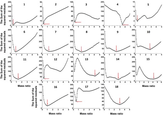
Sum of the squared residuals as a function of the mass ratio.
Based on our measurements, the maxima of the light curves are not equal for 11 target systems. So, the light-curve solution required a starspot on a component due to the asymmetry in the light curve’s maxima. The most probable explanation is that the magnetic activity of the components is causing the presence of the starspot(s), which are introduced with the O’Connell effect (O’Connell 1951, Sriram et al. 2017). Colatitude (Col.|$^\circ$|), longitude (Long.|$^\circ$|), angular radius (Radius|$^\circ$|), and the ratio of temperature (|$T_{\mathrm{spot}}/T_{\mathrm{star}}$|) are the characteristics that are commonly identified for a starspot (Table 4).
The target systems’ photometric light curve solutions. According to the columns’ order: The stars’ temperatures are denoted by |$T_{1,2}$|, their mass ratio by |$q=M_2/M_1$|, their orbital inclination by i, their fillout factor by f, their surface potential by |$\Omega _{1,2}$|, their luminosities by |$l_{1,2}/l_{\mathrm{tot}}$|, and their mean equivalent radius by |$r_{\mathrm{mean}1,2}$|.
| System | |$T_1$|(K) | |$T_2$|(K) | q | |$i^{\circ }$| | f | |$\Omega _{1,2}$| | |$l_1/l_{\mathrm{tot}}(V)$| | |$l_2/l_{\mathrm{tot}}(V)$| | |$r_{\mathrm{mean}1}$| | |$r_{\mathrm{mean}2}$| |
|---|---|---|---|---|---|---|---|---|---|---|
| 1 | 5396(32) | 5695(35) | 0.299(18) | 81.38(15) | 0.149(3) | 2.436(28) | 0.693(6) | 0.307(6) | 0.496(3) | 0.289(2) |
| 2 | 5912(39) | 5992(37) | 0.228(16) | 79.97(9) | 0.253(5) | 2.264(37) | 0.777(9) | 0.223(3) | 0.524(4) | 0.274(3) |
| 3 | 5802(29) | 6056(33) | 0.210(15) | 80.28(7) | 0.631(24) | 2.173(84) | 0.755(5) | 0.245(2) | 0.548(8) | 0.288(5) |
| 4 | 4800(33) | 4483(32) | 3.480(19) | 70.85(8) | 0.144(2) | 7.155(90) | 0.343(4) | 0.657(7) | 0.286(2) | 0.499(4) |
| 5 | 5214(38) | 4928(36) | 0.437(11) | 77.15(9) | 0.146(2) | 2.714(39) | 0.745(6) | 0.255(3) | 0.464(4) | 0.320(4) |
| 6 | 5957(40) | 5876(38) | 0.795(10) | 76.78(11) | 0.316(14) | 3.267(142) | 0.565(3) | 0.435(3) | 0.429(5) | 0.389(5) |
| 7 | 6091(35) | 6130(39) | 1.210(18) | 64.78(10) | 0.079(1) | 4.040(44) | 0.450(3) | 0.550(3) | 0.370(3) | 0.404(3) |
| 8 | 6050(40) | 6173(42) | 1.503(13) | 62.07(15) | 0.108(2) | 4.468(63) | 0.387(3) | 0.613(4) | 0.354(4) | 0.425(4) |
| 9 | 5789(37) | 5653(36) | 2.289(12) | 59.60(12) | 0.103(1) | 5.593(63) | 0.346(4) | 0.654(4) | 0.317(5) | 0.461(5) |
| 10 | 5433(31) | 5147(30) | 2.841(27) | 73.26(11) | 0.090(1) | 6.349(56) | 0.342(2) | 0.658(3) | 0.298(2) | 0.479(3) |
| 11 | 4940(35) | 4836(34) | 1.306(15) | 76.89(9) | 0.119(2) | 4.165(68) | 0.475(5) | 0.525(6) | 0.367(2) | 0.414(2) |
| 12 | 5509(38) | 5405(38) | 0.294(22) | 72.21(13) | 0.150(2) | 2.425(28) | 0.768(4) | 0.232(3) | 0.498(3) | 0.288(3) |
| 13 | 5749(26) | 5607(28) | 4.946(42) | 66.53(10) | 0.153(2) | 8.999(98) | 0.212(3) | 0.788(4) | 0.259(2) | 0.529(2) |
| 14 | 5051(31) | 4700(29) | 2.662(19) | 70.41(9) | 0.122(2) | 6.090(75) | 0.394(3) | 0.606(3) | 0.306(2) | 0.475(2) |
| 15 | 4987(20) | 4702(19) | 4.251(31) | 55.31(20) | 0.220(4) | 8.090(139) | 0.287(2) | 0.713(3) | 0.274(1) | 0.520(3) |
| 16 | 6207(46) | 6100(47) | 0.983(16) | 68.60(8) | 0.177(5) | 3.628(94) | 0.523(4) | 0.477(4) | 0.398(2) | 0.395(2) |
| 17 | 5848(32) | 5708(34) | 0.492(21) | 62.05(13) | 0.059(1) | 2.843(27) | 0.682(5) | 0.318(4) | 0.448(2) | 0.324(2) |
| 18 | 6706(33) | 6357(39) | 3.060(23) | 59.54(9) | 0.142(2) | 6.608(88) | 0.315(4) | 0.685(5) | 0.296(2) | 0.488(3) |
The starspot specifications of the target systems.
| System | Col.|$^{\circ }$| | Long.|$^{\circ }$| | Radius|$^{\circ }$| | |$T_{\mathrm{spot}}/T_{\mathrm{star}}$| | Component |
|---|---|---|---|---|---|
| 1 | 104(1) | 68(1) | 22(1) | 0.90(1) | Secondary |
| 6 | 107(1) | 56(1) | 16(1) | 0.84(1) | Secondary |
| 7 | 114(1) | 309(3) | 16(1) | 0.92(1) | Secondary |
| 8 | 114(1) | 290(2) | 16(1) | 0.87(1) | Secondary |
| 9 | 114(1) | 310(2) | 16(1) | 0.90(1) | Secondary |
| 10 | 104(1) | 290(2) | 14(1) | 0.84(1) | Secondary |
| 13 | 130(1) | 315(1) | 17(1) | 1.08(1) | Secondary |
| 14 | 80(1) | 317(2) | 19(1) | 0.89(1) | Secondary |
| 15 | 107(1) | 318(1) | 19(1) | 1.05(1) | Secondary |
| 17 | 110(1) | 220(1) | 21(1) | 0.74(2) | Secondary |
| 18 | 164(1) | 255(1) | 22(1) | 0.91(2) | Secondary |
We attempted to determine an acceptable theoretical fit using the initial values. We utilized the TESS filter, as well as the V filter from ASAS-SN, and the G, |$BP$|, and |$RP$| filters from Gaia in the analysis process. We focused on the TESS data for the light-curve analysis due to its low scattering. Afterward, we examined the results using the other data and filters.
Furthermore, we employed PHOEBE’s optimization tool to improve the output of light-curve solutions. According to the light-curve analysis, no target system showed |$l_3$|. Table 3 presents the outcomes of the light-curve solutions and Table 4 starspot specifications of the systems. Fig. 2 displays the TESS data and synthetic light curves of the binary systems. Fig. 2 displays systems 1 and 18 as examples of five filters used for target systems. The observational (ASAS-SN and Gaia) and synthetic light curves of other systems are included in the online supplement to the paper. The D views of the binary systems are displayed in Fig. 3.
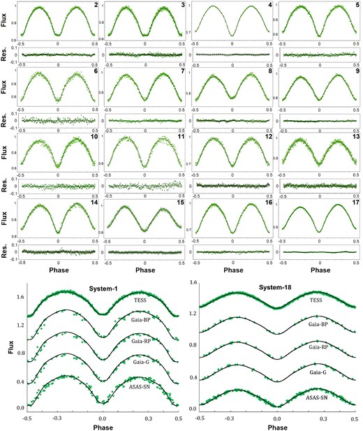
The green dots represent the observed light curves, while the synthetic light curves are produced using the light-curve solutions. In the upper panel, 16 target systems are shown using TESS data, while in the lower panel, systems 1 and 18 are displayed as examples using all filters.
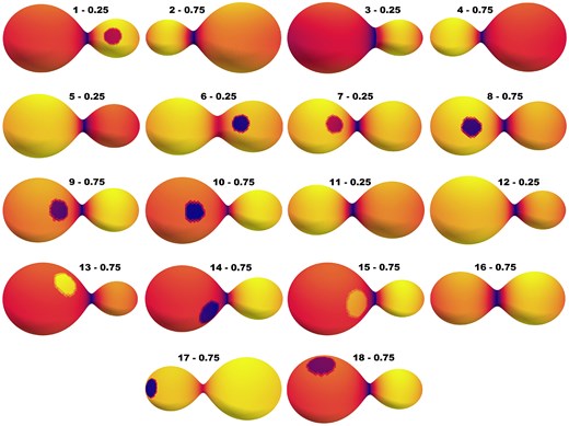
3D view of stars at phases 0.25 or 0.75. The numerals above the 3D representation of each system show the phase on the right and the star’s name on the left. The proper phase has been chosen in order to display the starspot that some target systems possess. The colours are based on modelling to show the temperature distribution on the surface of the star, and the darker the colour, the lower the temperature.
5 ABSOLUTE PARAMETERS
Contact binary system investigations have a variety of major objectives, one of which is to estimate the absolute parameters. We utilized the Gaia DR3 parallax to estimate the absolute parameters of the target systems (Poro et al. 2024c). When photometric data is available, this method will be an acceptable option due to the high level of parallax accuracy that Gaia DR3 provides (Li et al. 2021). However, there are a few limitations to estimating absolute parameters using Gaia DR3 parallax. It is required that the extinction coefficient |$A_V$| value be lower than approximately 0.4 (Poro et al. 2024d), and the RUWE value should not be more than 1.4 (Lindegren 2018), that these conditions are present for the target systems (see Tables 1 and 5). We calculated the |$A_V$| value from the 3D dust map (Green et al. 2019), and the RUWE was reported by the Gaia DR3.
Estimation of absolute parameters.
| System | |$M_1(M_\odot)$| | |$M_2(M_\odot)$| | |$R_1(R_\odot)$| | |$R_2(R_\odot)$| | |$L_1(L_\odot)$| | |$L_2(L_\odot)$| | |$M_{\mathrm{bol}1}(\mathrm{mag.})$| | |$M_{\mathrm{bol}2}(\mathrm{mag.})$| |
|---|---|---|---|---|---|---|---|---|
| 1 | 1.114(190) | 0.333(57) | 1.033(68) | 0.598(36) | 0.812(88) | 0.337(32) | 4.966(118) | 5.920(103) |
| 2 | 0.893(231) | 0.203(53) | 1.063(102) | 0.552(52) | 1.238(206) | 0.352(57) | 4.508(180) | 5.875(177) |
| 3 | 1.478(34) | 0.310(8) | 1.703(41) | 0.875(21) | 2.948(82) | 0.925(23) | 3.566(30) | 4.825(27) |
| 4 | 0.525(66) | 1.825(230) | 0.661(31) | 1.153(60) | 0.208(14) | 0.482(36) | 6.444(73) | 5.533(80) |
| 5 | 1.200(253) | 0.524(111) | 1.076(87) | 0.744(60) | 0.768(101) | 0.293(39) | 5.026(142) | 6.071(142) |
| 6 | 0.822(141) | 0.653(112) | 1.025(71) | 0.929(64) | 1.187(133) | 0.924(104) | 4.554(122) | 4.826(121) |
| 7 | 0.958(240) | 1.159(290) | 1.086(97) | 1.183(109) | 1.456(228) | 1.772(280) | 4.332(169) | 4.119(171) |
| 8 | 0.985(49) | 1.481(73) | 1.032(27) | 1.240(33) | 1.281(33) | 2.003(54) | 4.471(29) | 3.986(30) |
| 9 | 0.997(124) | 2.283(285) | 1.030(55) | 1.502(84) | 1.069(87) | 2.068(179) | 4.668(88) | 3.951(94) |
| 10 | 0.556(182) | 1.580(516) | 0.860(97) | 1.386(159) | 0.578(118) | 1.210(251) | 5.336(220) | 4.533(224) |
| 11 | 0.314(83) | 0.409(109) | 0.510(48) | 0.573(52) | 0.139(22) | 0.161(25) | 6.886(168) | 6.726(168) |
| 12 | 0.798(164) | 0.235(48) | 0.931(73) | 0.538(40) | 0.716(91) | 0.222(26) | 5.103(138) | 6.375(131) |
| 13 | 0.269(42) | 1.333(209) | 0.766(42) | 1.573(95) | 0.575(52) | 2.194(223) | 5.340(99) | 3.887(110) |
| 14 | 0.605(152) | 1.609(404) | 0.759(66) | 1.179(107) | 0.336(50) | 0.609(96) | 5.925(163) | 5.279(170) |
| 15 | 0.352(60) | 1.495(258) | 0.632(39) | 1.201(76) | 0.222(23) | 0.633(70) | 6.375(115) | 5.237(120) |
| 16 | 0.642(132) | 0.632(130) | 0.918(67) | 0.913(67) | 1.122(130) | 1.035(120) | 4.615(126) | 4.703(126) |
| 17 | 0.813(126) | 0.400(62) | 0.949(54) | 0.688(38) | 0.945(87) | 0.451(40) | 4.801(100) | 5.605(96) |
| 18 | 0.692(129) | 2.116(395) | 1.045(69) | 1.734(124) | 1.981(221) | 4.406(52) | 3.998(121) | 3.130(128) |
| System | |$M_{V1}(\mathrm{mag.})$| | |$M_{V2}(\mathrm{mag.})$| | |$log(g)_1(cgs)$| | |$log(g)_2(cgs)$| | |$a(R_\odot)$| | |$\Delta a(R_\odot)$| | |$logJ_0(g.cm^2/s)$| | |$A_V(\mathrm{mag.})$| |
| 1 | 5.131(108) | 6.015(96) | 4.457(131) | 4.407(127) | 2.076(118) | 0.014 | 51.429(139) | 0.285(1) |
| 2 | 4.566(173) | 5.921(172) | 4.336(195) | 4.262(195) | 2.022(173) | 0.014 | 51.173(211) | 0.065(1) |
| 3 | 3.641(25) | 4.863(23) | 4.145(31) | 4.045(31) | 3.073(24) | 0.070 | 51.560(37) | 0.035(1) |
| 4 | 6.851(54) | 6.145(56) | 4.518(96) | 4.576(99) | 2.311(97) | 0.000 | 51.759(90) | 0.029(1) |
| 5 | 5.248(128) | 6.412(124) | 4.454(160) | 4.414(159) | 2.322(161) | 0.006 | 51.645(159) | 0.058(1) |
| 6 | 4.605(116) | 4.889(115) | 4.331(134) | 4.317(134) | 2.388(136) | 0.001 | 51.616(126) | 0.150(1) |
| 7 | 4.366(166) | 4.148(167) | 4.348(185) | 4.356(187) | 2.932(242) | 0.007 | 51.898(185) | 0.328(1) |
| 8 | 4.510(23) | 4.010(25) | 4.404(44) | 4.422(44) | 2.916(48) | 0.003 | 51.982(35) | 0.069(1) |
| 9 | 4.745(82) | 4.054(87) | 4.411(100) | 4.443(103) | 3.254(135) | 0.009 | 52.137(90) | 0.307(1) |
| 10 | 5.491(212) | 4.780(212) | 4.314(237) | 4.353(239) | 2.890(310) | 0.008 | 51.791(243) | 0.066(1) |
| 11 | 7.222(151) | 7.114(150) | 4.520(196) | 4.533(195) | 1.387(122) | 0.006 | 51.031(196) | 0.057(1) |
| 12 | 5.238(128) | 6.537(120) | 4.402(156) | 4.348(153) | 1.868(127) | 0.001 | 51.183(169) | 0.172(1) |
| 13 | 5.424(94) | 3.999(104) | 4.099(115) | 4.169(121) | 2.966(155) | 0.016 | 51.470(112) | 0.287(5) |
| 14 | 6.211(150) | 5.744(153) | 4.459(183) | 4.502(187) | 2.481(206) | 0.002 | 51.794(184) | 0.165(1) |
| 15 | 6.689(105) | 5.701(109) | 4.383(128) | 4.454(130) | 2.308(133) | 0.003 | 51.551(124) | 0.036(1) |
| 16 | 4.636(121) | 4.736(120) | 4.320(152) | 4.318(152) | 2.309(157) | 0.004 | 51.519(151) | 0.139(1) |
| 17 | 4.869(95) | 5.697(89) | 4.394(116) | 4.365(115) | 2.120(109) | 0.005 | 51.415(119) | 0.065(1) |
| 18 | 3.979(119) | 3.136(124) | 4.240(137) | 4.285(143) | 3.542(219) | 0.023 | 51.997(135) | 0.124(1) |
This method estimates the system’s absolute magnitude (|$M_V$|) using the apparent magnitude of the system |$V_{\mathrm{system}}$|, distance from Gaia DR3, and |$A_V$|. We used the |$V^{\mathrm{mag.}}$| values reported by the TESS Input Catalogue, listed in Table 2. Then, using the |$l_{1,2}/l_{\mathrm{tot}}$| parameter obtained from the V filter in the light-curve solutions process, |$M_{V1}$| and |$M_{V2}$| are calculated. We estimated the absolute bolometric magnitude (|$M_{\mathrm{bol}1,2}$|) based on the Bolometric Corrections (|$BC_{1,2}$|) that were extracted from the Flower (1996) study. The radius of the stars in the binary systems is readily estimated using a relationship between |$M_{\mathrm{bol}}$| and luminosity (L). We considered |$M_{\mathrm{bol}\odot }$| as |$4.73^{\mathrm{mag.}}$| from the Torres (2010) throughout this estimating process. Also, by having the luminosity from this process and the effective temperature of the stars from the light-curve solution, the radius (R) of each star can be obtained. The semimajor axis |$a(R_{\odot })$| of each system is calculated using |$R_{1,2}$| and |$r_{\mathrm{mean}1,2}$| and averaging |$a_1(R_{\odot })$| and |$a_2(R_{\odot })$|. Then, having parameters |$a(R_{\odot })$|, |$P_{orb}$|, and q, it is possible to estimate the mass of each component through the well-known Kepler’s third law (equations 1 and 2):
The results of these estimations show that the difference between |$a_1(R_{\odot })$| and |$a_2(R_{\odot })$| was lower than |$\approx 0.1$| (Table 5), which is suitable for this method, and one of the signs of the appropriateness of light-curve analysis and input parameters (Poro et al. 2024c). Furthermore, based on the total mass, q, and P of each system, the orbital angular momentum (|$J_0$|) was calculated and presented in table 5 using the equation (3) from the Eker et al. (2006) study.
The estimated absolute parameters for the target binary systems are presented in Table 5.
6 DISCUSSION AND CONCLUSION
We present the light-curve analysis and absolute parameters’ estimations of 18 contact binary systems with orbital periods shorter than 0.5 d. We employed the TESS, Gaia, and ASAS-SN survey observations of these binary systems for our investigation. Based on the results, the following are presented as discussions and conclusions:
(a) Light-curve analysis was done using the PHOEBE Python code. The light-curve solutions of the 11 systems required the addition of a starspot. The stars in the target systems have a temperature range of 4643–6913 K. Also, the solutions show that the lowest effective temperature difference between the two stars is 39 K for system 7, and the highest is 351 K for system 14 (Table 6). The spectral category of the stars of the systems was also presented in Table 6 based on the Cox (2000) and Eker et al. (2018) studies.
Some conclusions regarding the target systems. |$\Delta T=T_1-T2$|: Effective temperature difference between component – Sp.: Spectral categorization of the stars – q or |$1/q$|: The results of this study for mass ratio – |$1/q^{*}$|: The Kouzuma method results for mass ratio – |$\Delta 1/q$|: The difference in mass ratio obtained by the Kouzuma method and this study’s results (|$1/q$|) – Subtype: The result of this study for each target system subtype – |$f_{cat.}$|: Fillout factor category of each system – |$M_{1,2i}$|: Initial mass of the components – |$M_{lost}$|: The result of mass lost of the system based on equation (10).
| System | |$\Delta T$| (K) | Sp. | |$1/q$| | |$1/q^{*}$| | |$\Delta 1/q$| | Subtype | |$f_{cat.}$| | |$M_{1i}$| (|${\rm M}_{\odot }$|) | |$M_{2i}$| (|${\rm M}_{\odot }$|) | |$M_{lost}$| (|${\rm M}_{\odot }$|) |
|---|---|---|---|---|---|---|---|---|---|---|
| 1 | –299 | G8-G6 | 0.299 | 0.311(44) | 0.012 | W | Shallow | 0.73 | 1.49 | 0.77 |
| 2 | –80 | G2-G0 | 0.228 | 0.259(43) | 0.031 | W | Medium | 0.40 | 1.67 | 0.98 |
| 3 | –254 | G3-G0 | 0.210 | 0.235(43) | 0.025 | W | Deep | 0.93 | 1.94 | 1.08 |
| 4 | 317 | K3-K5 | 0.287 | 0.329(43) | 0.042 | W | Shallow | 1.73 | 0.80 | 0.18 |
| 5 | 286 | K0-K2 | 0.437 | 0.435(44) | –0.002 | A | Shallow | 1.03 | 1.04 | 0.34 |
| 6 | 81 | G1-G2 | 0.795 | 0.794(43) | –0.001 | A | Medium | 0.55 | 1.46 | 0.53 |
| 7 | –39 | F8-F8 | 0.826 | A | Shallow | |||||
| 8 | –123 | G0-F8 | 0.665 | A | Shallow | |||||
| 9 | 136 | G3-G7 | 0.437 | 0.389(48) | –0.048 | W | Shallow | |||
| 10 | 286 | G8-K1 | 0.352 | 0.400(46) | 0.048 | W | Shallow | 1.31 | 1.37 | 0.54 |
| 11 | 104 | K2-K2 | 0.766 | 0.773(43) | 0.007 | W | Shallow | 0.12 | 1.17 | 0.57 |
| 12 | 104 | G8-G8 | 0.294 | 0.334(43) | 0.040 | A | Shallow | 0.38 | 1.47 | 0.82 |
| 13 | 142 | G5-G7 | 0.202 | 0.243(45) | 0.041 | W | Shallow | 0.82 | 1.79 | 1.01 |
| 14 | 351 | K1-K3 | 0.376 | 0.407(46) | 0.031 | W | Shallow | 1.53 | 0.85 | 0.17 |
| 15 | 285 | K1-K3 | 0.235 | 0.243(43) | 0.008 | W | Shallow | 1.18 | 1.29 | 0.62 |
| 16 | 107 | F7-F8 | 0.983 | A | Shallow | 0.33 | 1.57 | 0.62 | ||
| 17 | 140 | G3-G6 | 0.492 | 0.493(44) | 0.001 | A | Shallow | 0.44 | 1.51 | 0.74 |
| 18 | 349 | F3-F5 | 0.327 | 0.324(42) | –0.003 | W | Shallow | 1.72 | 1.87 | 0.78 |
(b) Kouzuma (2018) introduced a new method for estimating mass ratios in overcontact binary systems using light-curve derivatives. The technique is based on the relationship between the mass ratio and the time interval between specific extrema in the third derivative of the light curve. This approach is more direct than previous methods of estimating mass ratio, like q-search, and it requires only numerical differentiation and time interval measurement without the need for iterative procedures. The method was examined by the Kouzuma (2018) study on a number of the overcontact binary systems and showed that the estimated mass ratios for about 67 per cent of the samples matched their spectroscopic mass ratios within the estimated uncertainties. Additionally, about 95 per cent of the errors were within |$\pm 0.1$|. The outcome of this method provides the mass ratio as |$1/q$|. Kouzuma (2018) method estimates mass ratio q using a linear relation (equation 4):
which involves calculating a key parameter W, derived from the time intervals between the second extrema and the light curve’s third derivative.
The approach is particularly useful for systems where spectroscopic data is unavailable or too resource-intensive. It offers a reliable alternative or complementary way for mass ratio estimation using high-precision photometric data from missions such as TESS. Additionally, it yields reasonable uncertainty estimates, making it a valuable tool for analysing overcontact binaries and understanding more about their characteristics. However, despite the accuracy, this method does not work for some of the contact systems (Poro et al. 2024e). The Kouzuma (2018) study has presented the conditions for using this method; for example, two maxima should be observed in the second derivative of the light curve. Therefore, we should expect that this method will not provide an estimate for some contact binary systems, mostly those whose mass ratio is around 1 or whose orbital inclination is less than |$\approx 60^{\circ }$|.
We attempted to use the Kouzuma (2023) method to estimate the mass ratio for our systems and compared the results with the findings from light-curve analysis. Therefore, it was possible to use this method for 15 target systems. The method does not apply to the other eight systems since there was no appearance of a double peak in the second derivative of the light curve (Poro et al. 2024e). The results are listed in Table 6, and we compared them with our results. Table 6 (|$\Delta 1/q$|) shows that for our 15 systems, the mass ratio results obtained in this study are in good agreement with the third derivative method of the light curve. Fig. 4 shows the derivation process on the light curve of one of the systems as an example.
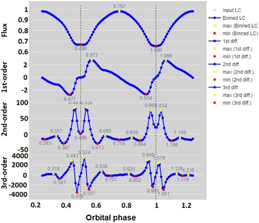
The light curve of 2MASS 00005760+0236413, and the first to third derivatives (top to bottom panels), respectively. The units of the panels on the vertical axis from top to bottom for 1st, 2nd, and 3rd orders are W m|$^{-2}$|, 10 W m|$^{-2}$| d|$^{-1}$|, and |$10^2$| W m|$^{-2}$| d|$^{-2}$|, respectively.
(c) The degree of contact between the companions in a binary system is measured by the fillout factor, often known as the contact parameter (f). The literature contains several definitions; however, the first was provided by Mochnacki & Doughty (1972) (equation 5):
where |$\Omega$| is the surface of the common envelope, and |$\Omega (L_1)$| and |$\Omega (L_2)$| denote the normalized potential of the surface passing through |$L_1$| and |$L_2$|, respectively. Overcontact binary systems have a fillout factor of |$0< f < 1$|. The |$f=0$| when the stars are just in contact and the potential at the surface of the star equals the potential at the inner Lagrangian surface, whereas the |$f=1$| when they are in complete contact and the potential at the surface of the star equals the potential at the outer Lagrangian surface.
In the light-curve solution, one of the two factors f or |$\Omega _{1,2}$| is considered as input and another is calculated. In this study, we used f for the analysis process, especially since searching for the f parameter in the range of 0–1 is much faster and more accurate than searching in a larger range for |$\Omega _{1,2}$| in the analysis process.
There are three categories for fillout factors of the contact binary systems: deep (|$f\ge 50~{{\ \rm per\ cent}}$|), medium (|$25~{{\ \rm per\ cent}} \le f < 50~{{\ \rm per\ cent}}$|), and shallow (|$f< 25~{{\ \rm per\ cent}}$|) eclipsing contact binary stars (Li et al. 2022). We have displayed the fillout factor category for each target system in Table 6.
(d) We used the Gaia DR3 parallax to estimate the absolute parameters (Poro et al. 2024c). The Li et al. (2021) study showed that the Gaia distance can be used to estimate the absolute parameters for most contact binaries. Li et al. (2021) employed a sample of 173 contact systems for this result, and they compared the reported distance from Gaia with the distance derived from the studies’ calculations.
There are some limitations to using the Gaia DR3 parallax to estimate absolute parameters, and in Poro et al. (2024c) discussed in detail. Additionally, this method can reveal if there were some problems in light-curve analysis. The Gaia DR3 parallax method calculations were done from the path of each star separately, so the semimajor axis |$a_{1,2}$| values of the stars can be different. So, the |$l_{1,2}$| and |$r_{\mathrm{mean}1,2}$| parameters that are used from the light-curve solution in the process of estimating the absolute parameters determine the values of |$a_{1,2}(R_{\odot })$|. |$l_{1,2}$| and |$r_{\mathrm{mean}1,2}$| depend on different parameters of the stars; for example, l is more dependent on the effective temperature of each star, and |$r_{\mathrm{mean}}$| is more related to the mass ratio and fillout factor. Considering that |$r_{\mathrm{mean}}$| is obtained from |$r_{\mathrm{mean}}=(r_{\mathrm{pole}}\times r_{\mathrm{side}}\times r_{\mathrm{back}})^{1/3}$| which is calculated from three different radii in the star’s Roche lobe geometry. The results of the Poro et al. (2024c) study indicated that an inappropriate input effective temperature of the stars could lead to not being close enough between |$a_1(R_\odot)$| and |$a_2(R_\odot)$|. Based on a sample of 48 systems and a histogram, the Poro et al. (2024c) study suggested that |$\Delta a=|a_1-a_2|$| in (|$R_\odot$|) unit should be approximately 0.1 or lower. A significant value of |$\Delta a$| may indicate issues in the parameters derived from light-curve analysis (Poro et al. 2024c).
Due to the increasing use of this method to estimate the absolute parameters of contact systems, a more reliable limit for the difference between |$a_1(R_\odot)$| and |$a_2(R_\odot)$| should be determined (Poro et al. 2024e). For this purpose, we collected a sample of contact systems from the literature that have estimated absolute parameters using the Gaia parallax and reported |$a_1(R_\odot)$| and |$a_2(R_\odot)$|, along with the systems of this study. So, we considered a total of 70 contact binary systems from five sources (Table 7). We placed |$a_1(R_\odot)$| and |$a_2(R_\odot)$| from the sample in Fig. 5 and generated a statistical linear fit on the data with uncertainties (equation 6). This linear fit is applicable for stellar radii lower than 5|$R_\odot$|.
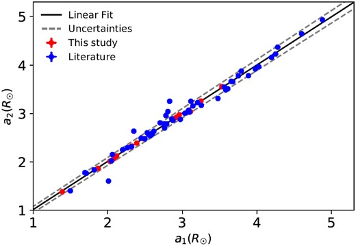
The relation between the |$a_1(R_\odot)$| and |$a_2(R_\odot)$| based on the results of 70 contact systems for which the estimation of absolute parameters with Gaia parallax method has been reported.
A sample collected from the literature for a discussion on estimating absolute parameters using the Gaia parallax.
| System | |$a_1(R_{\odot })$| | |$a_2(R_{\odot })$| | Ref. | System | |$a_1(R_{\odot })$| | |$a_2(R_{\odot })$| | Ref. | System | |$a_1(R_{\odot })$| | |$a_2(R_{\odot })$| | Ref. |
|---|---|---|---|---|---|---|---|---|---|---|---|
| TIC 432482096 | 2.083 | 2.069 | a | BO Ari | 2.318 | 2.315 | b | RR Cen | 4.249 | 4.228 | b |
| TIC 257469111 | 2.029 | 2.015 | a | BX Dra | 3.977 | 3.919 | b | RV CVn | 2.199 | 2.251 | b |
| TIC 70723515 | 3.108 | 3.038 | a | CU Tau | 2.873 | 2.857 | b | RV Psc | 3.654 | 3.663 | b |
| TIC 70761941 | 2.311 | 2.311 | a | DD Com | 2.062 | 2.152 | b | SS Com | 2.567 | 2.541 | b |
| TIC 117626504 | 2.319 | 2.325 | a | DN Boo | 3.609 | 3.511 | b | SW Lac | 2.448 | 2.491 | b |
| TIC 266907594 | 2.389 | 2.388 | a | DN Cam | 4.278 | 4.370 | b | UV Lyn | 3.094 | 3.029 | b |
| TIC 301790387 | 2.935 | 2.928 | a | EF Boo | 2.806 | 3.041 | b | UZ Leo | 3.886 | 3.781 | b |
| TIC 327938159 | 2.915 | 2.918 | a | EF Dra | 3.084 | 3.067 | b | V2364 Cyg | 4.600 | 4.647 | b |
| TIC 331742359 | 3.249 | 3.258 | a | EH Cnc | 2.618 | 2.634 | b | V369 Cep | 2.757 | 2.785 | b |
| TIC 200664816 | 2.886 | 2.894 | a | EI CVn | 2.349 | 2.636 | b | V402 Aur | 4.195 | 4.158 | b |
| TIC 201292881 | 1.390 | 1.384 | a | EQ Cep | 2.262 | 2.294 | b | V404 Peg | 2.829 | 3.253 | b |
| TIC 194507888 | 1.869 | 1.868 | a | GSC 3553–845 | 3.205 | 3.228 | b | V502 Oph | 3.142 | 3.157 | b |
| TIC 359437732 | 2.958 | 2.974 | a | GSC 804–118 | 2.499 | 2.478 | b | V530 And | 3.790 | 3.877 | b |
| TIC 202221727 | 2.480 | 2.482 | a | GSC 2936–478 | 2.701 | 2.808 | b | V604 Car | 3.253 | 3.168 | b |
| TIC 201353809 | 2.307 | 2.310 | a | GW Cnc | 1.712 | 1.766 | b | V842 Her | 2.780 | 2.959 | b |
| TIC 25694300 | 2.307 | 2.311 | a | GZ And | 1.819 | 1.837 | b | VZ Tri | 2.049 | 2.023 | b |
| TIC 434207067 | 2.118 | 2.123 | a | HH UMa | 2.583 | 2.586 | b | XY LMi | 3.583 | 3.487 | b |
| TIC 283428282 | 3.530 | 3.553 | a | HI Dra | 4.879 | 4.934 | b | EI Oct | 2.528 | 2.602 | c |
| AK Her | 3.114 | 3.253 | b | HI Pup | 2.790 | 2.786 | b | V336 TrA | 1.498 | 1.404 | c |
| AO Aqr | 3.477 | 3.311 | b | KIC 3221207 | 3.675 | 3.658 | b | NX Boo | 1.694 | 1.780 | c |
| AP Leo | 2.761 | 2.700 | b | MQ UMa | 3.562 | 3.547 | b | AP Dor | 3.034 | 3.004 | d |
| AQ Tuc | 4.024 | 3.968 | b | NO Cam | 2.594 | 2.569 | b | TIC 44559272 | 2.973 | 2.879 | e |
| V486 Gem | 3.751 | 3.779 | b | NR Cam | 2.010 | 1.606 | b | ||||
| AU Ser | 2.859 | 2.890 | b | OO Aql | 2.557 | 2.560 | b |
The range of uncertainty in Fig. 5 encompasses all 18 target systems in our investigation. 0.1 or lower has been determined by the Poro et al. (2024c) study as an appropriate value for the difference between |$a_1(R_\odot)$| and |$a_2(R_\odot)$| (|$\Delta a$|). Equation (6) and Fig. 5 show that the amount of uncertainty will increase or decrease with the |$a(R_\odot)$| values.
(e) We found that the target systems are W UMa eclipsing contact binary systems based on their light-curve solution parameters results like mass ratios, fillout factors, and orbital inclinations. Additionally, we estimated each companion star’s mass using the Gaia DR3 parallax method. However, the results presented in Tables 3 and 5 can be considered as approximations due to some modelling omissions, such as metallicity, atmosphere, effective temperature, etc., which are discussed in the PHOEBE-related references (Prša et al. 2016).
According to the definition of A and W subtypes of contact binaries (Binnendijk 1970) and outcomes from this study, we specified subtypes of the target systems (Table 6). The star in the A-type subtype systems is hotter and more massive. According to each component’s effective temperature and mass, seven of the systems are A-subtypes and eleven are W-subtypes.
(f) In W UMa-type contact binary systems, understanding the initial mass of two components provides critical insights into their evolutionary processes. We calculated the initial masses of the primary (|$M_{1i}$|) and secondary (|$M_{2i}$|) components for the most target contact binary systems using the method described by Yildiz & Doğan (2013).
First, the initial mass of the secondary component was estimated using equation (7) from the Yildiz & Doğan (2013) study,
where |$M_2$| is the current mass of the secondary, and |$M_L$| is derived from the mass–luminosity relation (equation 8).
The initial mass of the primary component was calculated using equation (9)
where the masses and luminosities are in solar units in equations (7), (8), and (9). Also, |$M_{\text{lost}}$| represents the mass lost in the system and |$\gamma$| is the ratio of |$M_{\text{lost}}$| to |$\Delta M$|:
We considered |$\gamma =0.664$| based on the Yildiz & Doğan (2013) results. The reciprocal mass ratio (|$1/{q_i}$|) serves as a physical constraint to determine the initial masses of the primary components. The results, including the initial masses of both components and the mass-loss of the 15 target systems, are presented in Table 6.
Understanding the evolution of W UMa-type binaries requires exploring the pathways leading to a star filling its Roche lobe. These pathways are primarily driven by nuclear and angular momentum evolution, both strongly influenced by the stellar mass (Hilditch, King & McFarlane 1989). The initial masses of the components are key parameters for understanding the formation and evolution of W UMa-type binaries.
As shown in Table 6, the initial masses of the primary components in our systems range from 0.1 to 1.7 |${\rm M}_{\odot }$|. The target systems with |$M_{1i}$| between 0.2 and 1.5 |${\rm M}_{\odot }$|, probably experience a relatively rapid loss of angular momentum (Tutukov, Dremova & Svechnikov 2004).
According to our calculations, the range of the initial secondary masses is 0.8–2.2 |${\rm M}_{\odot }$|. The secondary components of contact binary systems have an entirely different interior from that of normal main-sequence stars due to their initial mass being higher than the current mass (Yildiz & Doğan 2013). The difference between the masses of the secondary stars in our study and |$M_{2i}$| indicates significant mass-loss, and our results for 15 target systems are in agreement with the findings of Yildiz & Doğan (2013).
The results of the Yildiz & Doğan (2013) study are applicable to a large part of the contact binary systems. However, the method described in the Yildiz & Doğan (2013) study may not be appropriate for estimating the initial mass and mass-loss of some contact systems. Therefore, the values obtained for systems 7, 8, and 9 were not in the acceptable range and were not reported in Table 6.
(g) Recently, some studies have presented methods that include providing automatic light-curve solutions (e.g. Sun et al. 2020; Kobulnicky et al. 2022; Ding et al. 2023, 2024, Li et al. 2024). They reported a significant number of contact binary systems to obtain the main light curve parameters such as |$T_{1,2}$|, q, i, and f. This is an important goal when dealing with big data in space-based and ground-based observations. However, the process and output of these types of studies can be debatable (Poro et al. 2025). For example, results for five main parameters for system 18 were reported by Sun et al. (2020) and Li et al. (2024) studies. Sun et al. (2020) have discovered system 18 and reported |$T_1=6941$| K, |$T_2=5788$| K, |$q=0.11$|, |$f=0.48$|, and |$i=74.22$|. Also, Li et al. (2024) presented |$T_1=6639$| K, |$T_2=7569$| K, |$q=0.150(30)$|, |$f=0.174(57)$|, and |$i^\circ =58.5(1.4)$| as results for this system. Comparing the outcomes of the two studies with our findings reveals some differences. Sun et al. (2020) and this study outcome show |$T_{\mathrm{ratio}}>1$| but Li et al. (2024) reported |$T_{\mathrm{ratio}}<1$|. On the other hand, there is a large difference in the studies for the inclination parameter value. The values of |$T_{1,2}$| and i depend on the depth of the minima and the accuracy of the photometric data in the light-curve solution process. So, we reviewed the photometric data used in these investigations to find the possible cause of the significant differences in |$T_{\mathrm{ratio}}$| and i. Sun et al. (2020) presented the physical parameters of 2335 late-type contact binary systems using the Catalina Sky Survey (CSS) data. Sun et al. (2020) employed unfiltered photometry that was converted into |$V_{CSS}$| magnitude to standardize data to V-band magnitude. The Li et al. (2024) study presented the distributions of parameters of 11 111 short orbital period contact binary systems using ASAS-SN data in the V filter. Therefore, the Sun et al. (2020) and Li et al. (2024) studies used only a single band to analyse the light curves, which may cause the solution to be far from reality. Also, Sun et al. (2020) converted the photometric data from |$V_{CSS}$| to V band, and Li et al. (2024) reported i results with large uncertainties, which indicates that the used data are debatable. The Sun et al. (2020) and Li et al. (2024) studies reported |$\Delta T$| of 1153 and 930 K, respectively, although the depth of the minima in the data from various sources in this study does not show a big difference.
(h) Increasing the number of contact binary stars utilized in samples to examine the empirical relationships of parameters is one of the objectives of investigating new systems. Therefore, in this study, we collected a new sample to use in Section 6. Firsty, we reviewed a statistical study of the largest bibliographic compilation of stellar and orbital parameters sample presented by Latković, Čeki & Lazarević (2021). The sample of Latković et al. (2021) included 687 contact binary systems. So, we first checked all parameter values entered in this sample from the studies one by one and corrected many typos in entering values. After adding our 18 target systems and new studies from the literature, the new sample was provided by the 818 contact binary systems. Studies that used theoretical and automated methods for estimating some light-curve solution parameters were not utilized in this sample. The new sample contains: system name, orbital period (P), |$\mathrm{d}P/\mathrm{d}t$|, light-curve solutions’ parameters (q, i, f, |$T_{1,2}$|, |$r_{\mathrm{mean}1,2}$|), absolute parameters (|$M_{1,2}$|, |$R_{1,2}$|, |$L_{1,2}$|), presence or absence of third light (|$l_3$|) and starspot, system type (A or W), type of eclipse (partial or total), solver program, and type of observation (photometric or spectroscopic). Some examples of recent years’ studies contained in the sample are presented in Table 8. This sample is available in the paper’s online version and can be used for future investigations.
A part of the sample of 818 contact systems was used in this study. This sample is available in machine-readable form. The abbreviations SP and PH correspond to spectroscopic or photometric data, respectively.
| Parameter | Results | Results | Results | Results |
|---|---|---|---|---|
| System | V1197 Her | V840 LYR | V505 Lac | OP Boo |
| Subtype | W | W | W | A |
| Eclipse Type | Total | Total | Partial | Partial |
| |$P(d)$| | 0.26268 | 0.22131 | 0.32700 | 0.31145 |
| |$\mathrm{d}P/\mathrm{d}t$| | –0.02229 | – | – | – |
| Solver | WD | PHOEBE | WD | WD |
| SP or PH | PH | PH | PH | PH |
| q | 2.610 | 0.451 | 2.759 | 1.233 |
| |$1/q$| | 0.383 | 0.451 | 0.362 | 0.811 |
| |$i^{\circ }$| | 82.70 | 80.44 | 60.53 | 59.57 |
| |$a(R_{\odot })$| | 1.760 | 1.579 | 2.393 | 2.401 |
| f | 0.157 | 0.151 | 0.179 | 0.035 |
| |$r_1$| | 0.473 | 0.465 | 0.480 | 0.402 |
| |$r_2$| | 0.308 | 0.322 | 0.304 | 0.356 |
| |$T_1(K)$| | 5113 | 4820 | 5983 | 4852 |
| |$T_2(K)$| | 4973 | 4775 | 5857 | 5388 |
| |$M_1({\rm M}_{\odot })$| | 0.770 | 0.744 | 1.260 | 1.058 |
| |$M_2({\rm M}_{\odot })$| | 0.300 | 0.336 | 0.457 | 0.858 |
| |$R_1(R_{\odot })$| | 0.830 | 0.735 | 1.148 | 0.965 |
| |$R_2(R_{\odot })$| | 0.540 | 0.508 | 0.728 | 0.855 |
| |$L_1(L_{\odot })$| | 0.380 | 0.257 | 1.396 | 0.708 |
| |$L_2(L_{\odot })$| | 0.180 | 0.119 | 0.614 | 0.365 |
| |$l_3$| | No | No | Yes | No |
| Starspot | Yes | Yes | Yes | Yes |
| Ref. | a | b | c | d |
(i) We updated 2D empirical parameter relationships of contact binary systems using the new sample to display the target systems’ positions in comparison with them. The parameters relationship between the orbital period (P) and the primary stars’ mass (|$M_1$|), radius (|$R_1$|), luminosity (|$L_1$|), and temperature (|$T_1$|) was updated. Some contact systems that were reported third-party were ignored for the |$P-L_1$| relationship sample. Based on the results of the Latković et al. (2021) study, the systems with an orbital period of less than 0.5 d and an effective temperature of less than about 7000 K can be considered as W UMa-type binary systems. Therefore, we considered these results by Latković et al. (2021) and calculated the parameter relationships using linear fits (equations (11), (12), (13), (14), and Fig. 6).
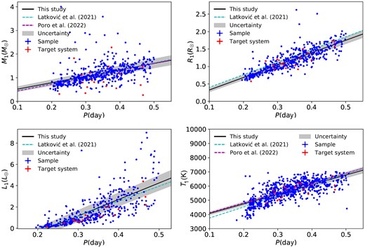
The position of the target systems (red colour) in the 2D diagrams of the empirical parameter relationships.
In equations (11)–(14), the mass, radius, and luminosity of the stars are expressed in terms of the Sun (|$M_\odot$|, |$R_\odot$|, |$L_\odot$|), while the temperature is represented in Kelvin and the orbital period with the day unit.
We have compared updated empirical parameter relationships with some others in the literature from the Latković et al. (2021) and Poro et al. (2022b) studies in Fig. 6.
We displayed the evolution state of the systems on the mass–radius (|$M-R$|) and mass–luminosity (|$M-L$|) diagrams based on the estimation of absolute parameters. According to the theoretical ZAMS and TAMS lines from the Girardi et al. (2000) study, the systems’ positions were shown in Fig. 7.
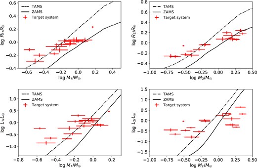
The position of the target systems (red colour) in the |$M-R$| and |$M-L$| diagrams. The ZAMS and TAMS lines come from the Girardi et al. (2000) study, and they define the range of main-sequence stars in terms of their evolutionary state.
ACKNOWLEDGEMENTS
This work was conducted with the cooperation of the Binary Systems of South and North (BSN, https://bsnp.info) project. RM is supported by Instituto de Astronomía Universidad Nacional Autónoma de México. This work has made use of data from the European Space Agency (ESA) mission Gaia (https://www.cosmos.esa.int/gaia), processed by the Gaia Data Processing and Analysis Consortium (DPAC, https://www.cosmos.esa.int/web/gaia/dpac/consortium). Funding for the DPAC has been provided by national institutions, in particular, the institutions participating in the Gaia Multilateral Agreement. This study uses data from the ASAS-SN variable stars database. ASAS-SN was founded by the Gordon and Betty Moore Foundation through grants GBMF5490 and GBMF10501 to Ohio State University and the Alfred P. Sloan Foundation grant G-2021-14192. This work includes data from the TESS mission observations. The NASA Explorer Program provides funding for the TESS mission. This paper used some information from the American Association of Variable Star Observers (AAVSO). We appreciate the contributions of Ehsan Paki in the analysis process.
DATA AVAILABILITY
The sample used in this study is available in an online machine-readable format.
Footnotes
Zwicky Transient Facility.
General Catalogue of Variable Stars.
AAVSO Photometric All-Sky Survey.
Variable Star Index, https://www.aavso.org/vsx/
Cross-match catalog of 17 841 723 of Gaia DR3 sources.
