


ABSTRACT
SN 2023tsz is a Type Ibn supernova (SN Ibn), an uncommon subtype of stripped-envelope core-collapse supernovae (SNe), discovered in an extremely low-mass host. SNe Ibn are characterized by narrow helium emission lines in their spectra and are believed to originate from the collapse of massive Wolf–Rayet (WR) stars, though their progenitor systems still remain poorly understood. In terms of energetics and spectrophotometric evolution, SN 2023tsz is largely a typical example of the class, although line profile asymmetries in the nebular phase are seen, which may indicate the presence of dust formation or unshocked circumstellar material. Intriguingly, SN 2023tsz is located in an extraordinarily low-mass host galaxy that is in the second percentile for stripped-envelope SN host masses and star formation rates (SFRs). The host has a radius of 1.0 kpc, a g-band absolute magnitude of |$-12.72 \pm 0.05$|, and an estimated metallicity of |$\log (Z_{*}/{\rm Z}_{\odot }) \approx -1.6$|. The SFR and metallicity of the host galaxy raise questions about the progenitor of SN 2023tsz. The low SFR suggests that a star with sufficient mass to evolve into a WR would be uncommon in this galaxy. Further, the very low metallicity is a challenge for single stellar evolution to enable H and He stripping of the progenitor and produce an SN Ibn explosion. The host galaxy of SN 2023tsz adds another piece to the ongoing puzzle of SNe Ibn progenitors, and demonstrates that they can occur in hosts too faint to be observed in contemporary sky surveys at a more typical SN Ibn redshift.
1 INTRODUCTION
Type Ibn supernovae (SNe Ibn) are a subclass of supernovae (SNe) that are characterized by the presence of narrow helium (He) emission lines in their spectra but the absence of strong hydrogen (H) features (e.g. Gal-Yam 2017; Smith 2017). These spectral properties are explained by the interaction of SN ejecta with He-rich, but H-poor, circumstellar material (CSM). The first SN Ibn was observed in 1999 (SN 1999cq; Matheson et al. 2000). However, the label was not coined until the analysis of SN 2006jc (Foley et al. 2007; Pastorello et al. 2007), which is considered the prototypical SN Ibn. Despite nearly two decades since their identification, there are still questions about the nature of their progenitors. These questions persist due to the lack of a confirmed direct detection of an SN Ibn progenitor as this type is relatively rare, with only 66 classified to date.1 It was estimated by Maeda & Moriya (2022) that they make up around 1 per cent of core-collapse (CC) SNe, with an observed rate of |$3{{\, \rm per\, cent}}$| (Perley et al. 2020).
The original progenitor suggested for the prototypical SN Ibn, SN 2006jc was an H-poor massive Wolf–Rayet (WR) star embedded in an He-rich CSM (Pastorello et al. 2007; Tominaga et al. 2008). Such progenitors are proposed for SNe Ibn, as the mass-loss that WR stars undergo prior to explosion can explain the properties seen in SN Ibn light curves (Maeda & Moriya 2022). This progenitor model is supported by the fact that the majority of SNe Ibn are found in active star-forming regions (e.g. Pastorello et al. 2015a; Taddia et al. 2015). However, there is a notable exception, PS1-12sk, which was discovered in the outskirts of an elliptical galaxy in a region with a low star formation rate (SFR; Sanders et al. 2013; Hosseinzadeh et al. 2019). Another proposed progenitor for SNe Ibn is a low-mass, |${\lesssim} 5\, {\rm M}_{\odot }$|, He star likely arising from a binary system. In this scenario, binary interactions are the cause of the mass-loss that creates the CSM prior to the explosion. The SN Ibn then arises from either the CC of the He star, or an explosion triggered by the merger of the He star and its binary companion (Maund et al. 2016; Dessart, Hillier & Kuncarayakti 2022; Dong et al. 2024). Such a progenitor could be more likely in an older stellar population. It is also plausible that multiple progenitor channels could lead to SNe that would be classified as an SN Ibn, such as the confirmed case of an SN IIb that exploded inside a dense CSM and appeared to be an SN Ibn (Prentice et al. 2020). Consequently, the nature and homogeneity of SN Ibn progenitors remain uncertain.
Compared to most CC SNe, which are powered primarily through the decay of |$^{56}{\rm Ni}$| produced during the explosion, a combined nickel decay and CSM interaction model is required to explain the light curves of SN Ibn (Clark et al. 2020). The CSM interaction is dominant at early times of SNe Ibn evolution, and is thought to explain their shorter time-scales for both the rise and decline of their light curves. These shorter time-scales make SN Ibn observationally rare as they are harder to characterize upon discovery, and are particularly hard to capture on their rise to the peak. The current generation of all-sky surveys, which are observing at higher cadences than previous surveys, will help to find and characterize SNe Ibn earlier in their evolution allowing improved probing of their physics.
The focus of this paper is the SN Ibn SN 2023tsz. It was discovered by the Gravitational-wave Optical Transient Observer (GOTO; Dyer et al. 2022, 2024); Steeghs et al. 2022) on 2023 September 28 and reported to the Transient Name Server under the name GOTO23anx (Godson et al. 2023). There was a prior non-detection and two detections from All-Sky Automated Survey for Supernovae (ASAS-SN; Shappee et al. 2014; Kochanek et al. 2017) on 2023 September 13, 19, and 25, respectively. The SN is associated with a faint galaxy, a possible satellite of LEDA 152972, located 33 arcsec from its centre, visible in the Dark Energy Spectroscopic Instrument (DESI) Legacy Survey Data Release 9 (DR9) images (Dey et al. 2019) as shown in Fig. 1. It is also the first object to be discovered, reported (Godson et al. 2023), and classified (Pursiainen et al. 2023c) entirely by the GOTO Collaboration.
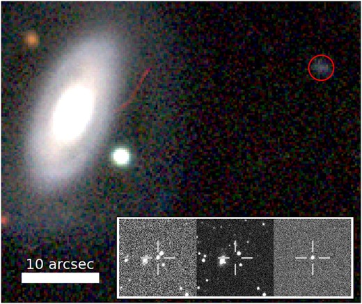
Image showing the host of SN 2023tsz (circled) and its immediate surroundings, including LEDA 152972. The image was created using g, r, and i observations from DR9 of the DESI Legacy Survey (Dey et al. 2019). The circle is the radius around SN 2023tsz’s host that contains 99 per cent of its light in the g band. The three image cut-outs in the bottom right of the image show the science (left), template (middle), and difference (right) images from GOTO that were used to discover SN 2023tsz. The GOTO science image was taken |$+3.2$| d with respect to our estimate of the peak (see text).
This paper is structured as follows: Section 2 presents the observations and data reduction methods; Section 3 presents the analysis of the data; Section 4 discusses the implications of our analysis; and Section 5 concludes our findings. Throughout this paper, we have corrected for a Milky Way extinction of |$E ({B-V})$| = 0.036 mag (Schlafly & Finkbeiner 2011). When analysing the spectra in Section 3.2 there is no evidence for significant host extinction. We assume a flat Λ cold dark matter (ΛCDM) cosmology with |$\Omega _{\rm m}$| = 0.31 and |$H_{0}$| = 67.66 km s−1 Mpc−1 (Planck Collaboration VI 2020). In the absence of host lines, we adopt the redshift value of z = 0.028, derived from spectrum template matching using the Supernova Identification (snid) code (Blondin & Tonry 2011), see Section 3.2. Using this cosmology and redshift, we calculate a luminosity distance for SN 2023tsz of 130 Mpc.
2 OBSERVATIONS AND DATA REDUCTION
In addition to GOTO L band (described in Steeghs et al. 2022), photometry of SN 2023tsz was collected in bands |$ugriz$| using the Liverpool Telescope (LT; Steele et al. 2004), the Rapid Eye Mount (REM) telescope (Covino et al. 2004), and Las Cumbres Observatory (LCO; Brown et al. 2013) Global Telescope Network. The data from LT and LCO were provided already pre-reduced for bias, dark, and flat-field corrections using their own pipelines (McCully et al. 2018). The data from REM telescope were reduced using our own pipeline. The light curves from these observations were calculated using the photometry-sans-frustration (psf) pipeline (Nicholl et al. 2023) making use of the inbuilt template subtraction of psf. Further photometry was collected in the near-ultraviolet (NUV) bands |$uvm2$|, |$uvw2$|, and |$uvw1$| with the Neil Gehrels Swift Observatory (Swift) Ultraviolet and Optical Telescope (UVOT; Roming et al. 2005), g from ASAS-SN, and o from the Asteroid Terrestrial-impact Last Alert System (ATLAS; Tonry et al. 2018; Smith et al. 2020). The ASAS-SN light curve was generated using their Sky Patrol service.2 The ATLAS light curve was generated using their forced photometry server (Shingles et al. 2021). The light curves from Swift UVOT were reduced using a 7 arcsec aperture to extract the photometry. This aperture was used due to a slight issue with Swift that caused smearing of the sources on the images (Cenko 2023).
Spectra of SN 2023tsz were obtained using the Alhambra Faint Object Spectrograph and Camera (ALFOSC) on the Nordic Optical Telescope (NOT), the Himalayan Faint Object Spectrograph Camera (HFOSC) on the Himalayan Chandra Telescope (HCT), the ESO Faint Object Spectrograph Camera 2 (EFOSC2) on the New Technology Telescope (NTT) at La Silla Observatory, taken by the extended Public ESO Spectroscopic Survey for Transient Objects plus (ePESSTO+; Smartt et al. 2015), and the Optical System for Imaging and low-Intermediate-Resolution Integrated Spectroscopy plus (OSIRIS+) on the Gran Telescopio Canarias (GTC). The data from ALFOSC were reduced using the pynot-redux reduction pipeline.3 The spectroscopic data from HFOSC were reduced in a standard manner using the packages and tasks in iraf with the aid of the python scripts hosted at redpipe (Singh 2021). The data from EFOSC2 were reduced using the pessto pipeline4 (Smartt et al. 2015). GTC optical spectra from OSIRIS+ were reduced following the routines in Piscarrera et al. (in preparation), based on pypeit (Prochaska et al. 2020). The spectral log is provided in Table A1.
Photometry of the host of SN 2023tsz was obtained from the Kilo-Degree Survey (KiDS; de Jong et al. 2015) in the u, g, r, and i bands, and from the VISTA Kilo-degree Infrared Galaxy Survey (VIKING; Edge et al. 2013) in the z band, detailed in Table A2. We also obtain upper limits from the Galaxy Evolution Explorer (GALEX; Martin et al. 2005) in the FUV and NUV bands, and the Wide-field Infrared Survey Explorer (WISE; Wright et al. 2010) in the WISE 1, 2, 3, and 4 bands. Finally, one epoch of ALFOSC V-band imaging polarimetry was obtained. The data were reduced and analysed following Pursiainen et al. (2023a).
3 ANALYSIS
3.1 Photometry
The multiband light curve of SN 2023tsz is shown in Fig. 2. Only the ASAS-SN g band had pre-peak observations, one a non-detection and the other a detection. This is due to the fact that SN 2023tsz was discovered as it exited solar conjunction, resulting in a late discovery and corresponding poor pre-peak observations. The decline was well sampled in multiple bands up to |${\sim} 40$| d post-peak, with later epochs sampled in g, r, and i. We define our peak epoch as the peak in the g band obtained from fitting a third-order polynomial to the data within |${\pm} 20 \, {\rm d} $| of the observed peak. This fitting gave us a peak date of MJD |$60212\pm 5$|. The large error on the time of the peak is due to the lack of constraining observations; going forward we adopt MJD 60212 as our peak date and use this for phase = 0. To estimate its decline rate in 15 d increments post-peak, we performed a linear regression on the data. These 15 d increments were chosen to investigate the visible flattening of the light curve, and to allow for comparison to other SN Ibn from Hosseinzadeh et al. (2017). The results of this are shown in Fig. 2. In the sample analysis of Hosseinzadeh et al. (2017), decline rates were estimated mostly in the R band, closely matched with our r-band observations. Unfortunately, determining the r-band peak brightness is difficult given our data coverage. The observed r-band peak was at +4.76 d when the SN was |$-19.03 \pm 0.03$| mag. The r-band decline rate in the first 15 d post-peak is |$0.145 \pm 0.002$| mag d−1, which if we extrapolate back to the peak makes the estimated peak r-band absolute magnitude of SN 2023tsz |$-19.7 \pm 0.7$| mag. This estimate is likely to be at an epoch before the true r-band peak as the SN is cooling and so would peak in the g band earlier than the r band. It is also unlikely that the SN declines at this rate immediately from the peak. Therefore, we consider this value as an upper limit on the magnitude. We show the range of peak magnitudes and the initial decline rate alongside a sample of other SN Ibn in Fig. 3. The figure shows that SN 2023tsz is slightly brighter and faster than the majority of the other SN Ibn from Hosseinzadeh et al. (2017), but is well within the distribution.
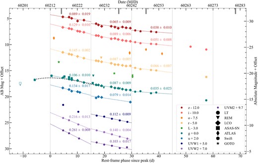
The multiband light curve of SN 2023tsz. In the legend, the number denotes the offset applied to the values in that filter. The third-order polynomial used to fit the peak date in the g band is shown by the black dotted curve. Dashed lines are used to show the light curve decline in each band over 15 d intervals after the peak. The decline rate for each interval (in mag d−1) is indicated on the plot next to the dashed line. Each 15 d interval is shown by the vertical light grey lines. We only fit the decline if there are at least three observations in the 15 d increment. The thick grey lines at the top of the plot represent the epochs when spectroscopic observations were obtained.
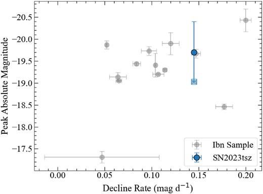
The initial 15 d post-peak decline rate and observed peak absolute magnitude of SN 2023tsz compared with other SNe Ibn. The two markers for SN 2023tsz encapsulate the uncertainty from not capturing the peak in the r band. The filled marker is an estimate of the peak by extrapolating the decline rate back to the epoch of the g-band peak, and the open square symbol is a certain lower limit on the absolute magnitude from the r-band observation at +4.76 d. Although we are comparing r-band observations to an R-band data set, differences between the filter throughputs are not at a level to change our inferences. The data for the SNe Ibn sample are from Hosseinzadeh et al. (2017).
The bolometric light curve was created using the superbol routine (Nicholl 2018). superbol works by fitting polynomial light-curve models to each band independently and then interpolating the magnitudes to the times of observation in a defined reference band before using them to fit blackbody models. As the g band has the most observations, and the only pre-peak observations, we used it as our reference band. In bands where we do not have late-time coverage (all bands except g, r, and i), we assume that the colour relative to the g band remains constant at the last measured epoch for that band. The temperatures of the first two epochs, which had only g-band data, were estimated by extrapolating the temperature curve with a second-degree polynomial. This was done as at these epochs only g-band photometry was obtained resulting in poor temperature estimates from fitting the bolometric light curve. All bands in which observations were obtained, other than the GOTO L band, were used to generate the bolometric light curve. The output of this routine was then smoothed by taking the error-weighted average of the bolometric luminosity (|$L_{\mathrm{bol}}$|), blackbody temperature (|$T_{\mathrm{BB}}$|), and blackbody radius (|$R_{\mathrm{BB}}$|) for each individual day of observations. The full bolometric light curve, along with the corresponding |$T_{\mathrm{BB}}$|, and |$R_{\mathrm{BB}}$| are presented in Fig. 4. The error in the distance was not considered when estimating the errors in the bolometric luminosity.
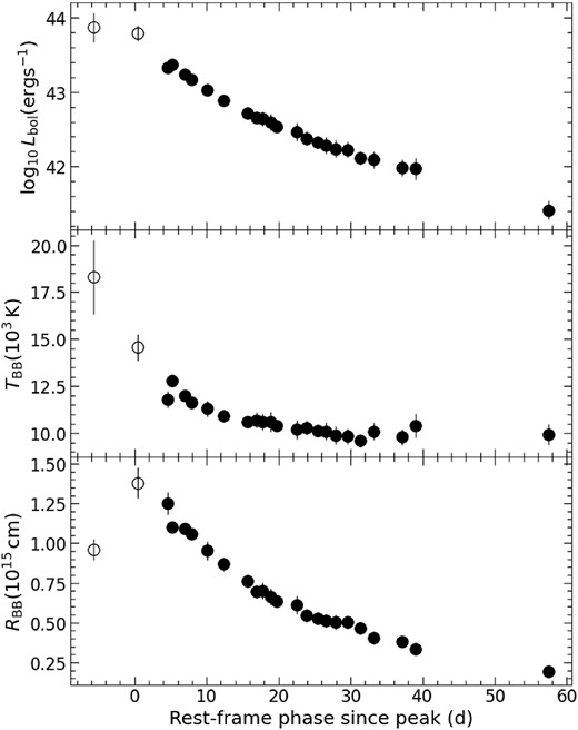
The bolometric light curve (top), blackbody temperature (middle), and blackbody radius (bottom) of SN 2023tsz over all observational epochs. For the epochs that only have g-band observations, the markers are unfilled.
We fit to the bolometric light curve the semi-analytical models of Chatzopoulos, Wheeler & Vinko (2012) for a combined CSM interaction and |$^{56} {\rm Ni}$| decay (CSM + Ni) model, using an emcee Bayesian analysis (Foreman-Mackey et al. 2013). We set the power-law index for the inner density profile of the ejecta as |$\delta =1$|, the power-law index for the outer component of the ejecta as |$n=10$|, the power-law index of the CSM as |$s=0$|, and the optical opacity of the CSM as |$\kappa =0.2$| cm2 g−1. These values were chosen to allow for a comparison to the work of Pellegrino et al. (2022a, b). We use a constant density CSM as, in the model we use, the density profile is degenerate with the radius of the star, and changing the density will effectively only affect the radius. The radius of the progenitor was chosen to be |$R_{0}=1.25 \times 10^{12}$| cm and the expansion velocity of the ejecta |$v=10\,000$| km s−1, aligning with the values used in Chatzopoulos et al. (2012). We constrained the explosion epoch to MJD |$60203.63 \pm 2.99$|. This explosion epoch uses the non-detection, at MJD 60200.64, and first detection, at MJD 60206.62 from ASAS-SN, as its bounds. The best-fitting model can be seen in Fig. 5 with the best-fitting model parameters presented in Table 1. Our first two data points only provide an estimate of the bolometric luminosity as they are from observations only in the g band and an extrapolated temperature. We have assumed that this temperature would decrease from the first observation, as is the case in standard Type II SNe. However, it has been observed that some rise in temperature after explosion (Hiramatsu 2022; Hiramatsu et al.2023).
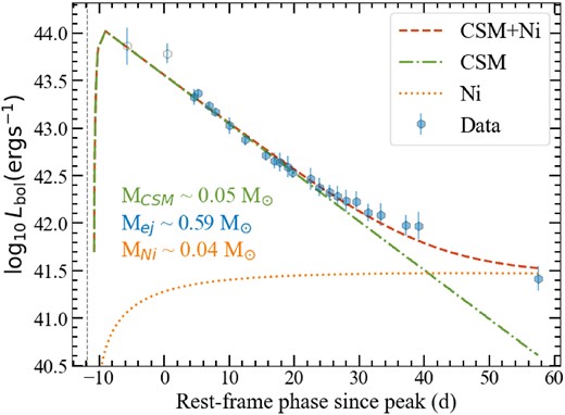
The best-fitting combined CSM + Ni model to the bolometric light curve of SN 2023tsz using the models of Chatzopoulos et al. (2012). For the epochs that only have g-band observations, the markers are unfilled. The individual CSM and Ni models are shown by the dash–dotted and dotted lines, respectively. The combined model is shown by the dashed red line. The best-fitting CSM (MCSM), ejecta (Mej), and Ni (MNi) masses are shown in the plot. The vertical dashed line shows the epoch of the ASAS-SN non-detection.
The best-fitting parameters for the CSM + Ni model.
| Parameter | Description | Value |
|---|---|---|
| |$M_{\mathrm{CSM}}$| (|${\rm M}_{\odot }$|) | CSM mass | |$0.05^{+0.05}_{-0.02}$| |
| |$M_{\mathrm{ej}}$| (|${\rm M}_{\odot }$|) | Ejecta mass | |$0.59^{+0.69}_{-0.38}$| |
| E (|$10^{51}$| erg) | Total energy of the SN | |$0.35^{+0.13}_{-0.12}$| |
| |$\dot{M}$| (|$10^{-4} \, {\rm M}_{\odot }$|) | Progenitor mass-loss rate | |$2.23^{+4.08}_{-1.66}$| |
| |$t_{\mathrm{expl}}$| (d) | Time of explosion relative to peak | |$-10.39^{+2.11}_{-1.49}$| |
| |$M_{\mathrm{Ni}}$| (|${\rm M}_{\odot }$|) | Total mass of nickel produced | |$0.04^{+0.01}_{-0.01}$| |
3.2 Spectra
The spectral time series of SN 2023tsz is compared to example SNe Ibn with spectra taken at similar epochs in Fig. 6. snid (Blondin & Tonry 2011) was used to match the initial NOT spectrum of SN 2023tsz to SNe template spectra and found a best match with an SN Ibn at a redshift of z = 0.028, which we choose to adopt for the redshift in our analysis. This template matching, along with manual inspection of the lines present in the spectrum, gave rise to the reported classification based on similarity to several prominent known SN Ibn, also shown in Fig. 6. Investigating the He lines in the spectrum obtained at |$+36.3$| d found a redshift value of |$0.0260\!-\!0.0265$|. This is a difference of |$450\!-\!600$| km s−1, which could be partially due to an inherent offset of the line. This would result in a luminosity distance of 120 Mpc and bolometric luminosity 17 per cent lower than our values obtained with z = 0.028. Our adopted redshift value differs from the redshift value for LEDA 152972 of z = 0.3515 (Liske et al. 2015). This implies a difference of 2200 km s−1 in recession velocity, significantly above the escape velocity expected of LEDA 152972, suggesting a chance alignment with the host of SN 2023tsz, rather than them being gravitationally bound. However, without narrow host lines, we cannot rule this out. The spectra show no presence of suppressed blue emission so we conclude there is no evidence for significant host extinction.
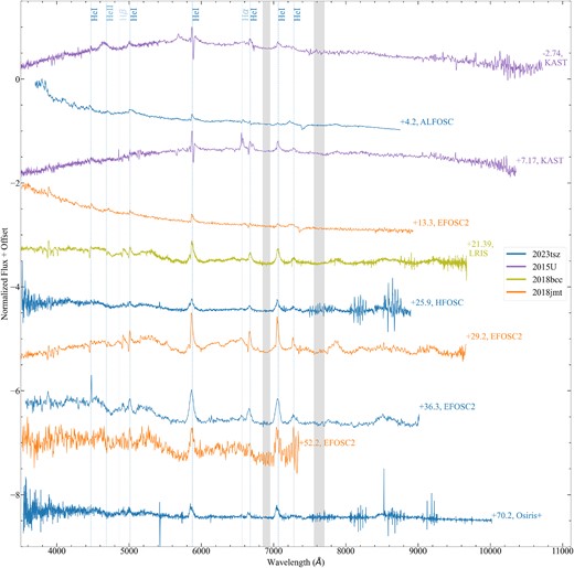
The spectroscopic time series of SN 2023tsz compared to the SN Ibn 2015U (Shivvers et al. 2016), 2018bcc (Karamehmetoglu et al. 2021), and 2018jmt (Chasovnikov et al. 2018). Spectra for these three SNe were obtained from the Weizmann Interactive Supernova Data Repository (Yaron & Gal-Yam 2012). The phase relative to the peak is shown next to each spectrum. Additionally, the instrument used to obtain each spectrum is listed. The He i, He ii, |${\rm H} \, \alpha$|, and |${\rm H} \, \beta$| features are marked by dashed lines, and tellurics are shown by the shaded regions. The spectra are shown in the rest frame of the SN.
The most prominent spectral features across all the spectra are the He i 5876, 6678, and 7066 Å lines. To investigate these lines, we fit a Gaussian emission and absorption component to reproduce the P Cygni profile, along with an additional Lorentzian emission component to account for the broad wings of the lines, to each line. This fitting was performed over a range extending 6000 km s−1 on each side of the line centre. The best-fitting values for each of these components were then determined using an emcee Bayesian analysis (Foreman-Mackey et al. 2013). Additionally, for the He i 5876 and 7066 Å lines in the |$+35.3$| and |$+70.2$| d spectra, we performed the same analysis with two Gaussian emission components (shown in Fig. 7) to investigate the noticeable blue asymmetry of the spectral features, likely due to a suppression of the red wing of the feature (in the |$+70.2$| d spectrum). In the classification spectrum, the most prominent line is the He i 5876 Å. In this line, we observe a significant P Cygni profile, with the profile minimum blueshifted by |$-1140^{+100}_{-180}$| km s−1. We do not find a fit to a P-Cyqni profile in the other spectra.
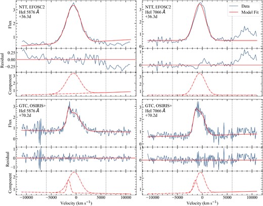
Line fitting of the He i 5876 Å line (left) and He i 7066 Å line (right) for the spectra obtained from the NTT (top) and the GTC (bottom). Each line is fit with two Gaussian profiles, for the NTT spectra the best fit was found to be with a single Gaussian. For each individual plot, the top panel shows the combined profile over the spectral feature, the middle panel shows the residuals, and the bottom panel shows the two individual Gaussian components.
The He i 5876 Å line becomes more prominent along with the He i 6678 and 7066 Å lines up to at least |$+36.3$| d post-peak. These strong He i lines are characteristic of typical SNe Ibn. The lines do weaken again at |$+70.2$| d post-peak, but still remain the most prominent features. At all times after the initial classification epoch, the emission component of these lines dominates over the blueshifted absorption component.
In the |$+70.2$| d spectrum, the He i lines appear to have a noticeable blue asymmetry. This asymmetry was confirmed by comparing fits of the lines in this spectrum to fits of the same lines in the |$+36.3$| d spectrum. The fits for the He i 5876 and 7066 Å lines are shown in Fig. 7. The features in the |$+36.3$| d spectrum are well fit by a single Gaussian with no evident second peak and so we determine such a component is not required. In the |$+70.2$| d spectrum, the same lines are best fit by two Gaussian components, a dominant Gaussian component and an additional, smaller, narrower Gaussian component on the blue side of the dominant Gaussian. In both cases the centre of the dominant Gaussian was fixed for each spectrum. The results of these fits are shown in Table 2.
The best-fitting parameters to the He i 5876 Å and He i 7066 Å lines of the |$+36.3$| and |$+70.2$| d spectra.
| Parameter | |$+36.3$| d spectrum | |$+70.2$| d spectrum | ||
|---|---|---|---|---|
| 5876 Å | 7066 Å | 5876 Å | 7066 Å | |
| Primary peak centrea (|$10^2$| km s−1) | –5.40|$^{+0.31}_{-0.32}$| | –3.90|$^{+1.77}_{-1.12}$| | ||
| Primary amplitude (erg s−1 cm−2 Å) | 6.58|$^{+0.22}_{-0.21} \, $||$\times \, 10^{-15}$| | 5.30|$^{+0.12}_{-0.12} \,$||$\times \, 10^{-15}$| | 4.55|$^{+0.45}_{-0.64} \, $||$\times \, 10^{-16}$| | 3.81|$^{+0.32}_{-0.49} \, $||$\times \, 10^{-16}$| |
| Primary FWHM (|$10^3$| km s−1) | 3.40|$^{+0.11}_{-0.10}$| | 2.75|$^{+0.07}_{-0.07}$| | 2.87|$^{+0.21}_{-0.27}$| | 2.17|$^{+0.27}_{-0.22}$| |
| Secondary peak centre (km s−1) | – | –1.49|$^{+0.06}_{-0.05} \, $||$\times \, 10^3$| | –1.38|$^{+0.15}_{-0.09} \, $||$\times \, 10^3$| | |
| Secondary amplitude (erg s−1 cm−2 Å) | – | 8.32|$^{+4.63}_{-2.37} \, $||$\times \, 10^{-17}$| | 1.39|$^{+0.24}_{-0.22} \, $||$\times \, 10^{-16}$| | |
| Secondary FWHM (km s−1) | – | 8.55|$^{+2.75}_{-2.02} \, $||$\times \, 10^2$| | 1.10|$^{+0.36}_{-0.19} \, $||$\times \, 10^3$| | |
The same peak centre was fit for both spectral features within each spectrum.
3.3 Polarimetry
The NOT/ALFOSC V-band polarimetry of SN 2023tsz taken at |$+15.6$| d appears to be consistent with zero polarization, as shown in Fig. 8. For the SN, we find Stokes parameters |$Q=-0.36\pm 0.28$| and |$U=0.34\pm 0.29$|, but the ALFOSC field of view also covers two nearby bright stars, which are perfectly consistent with the measured polarization of the SN. Based on the Gaia parallaxes from the Data Release 3 (Gaia Collaboration 2023), the stars are |$\gt 150$| pc above the Milky Way plane, and as such, they probe the full Galactic dust column and can be used to measure the Galactic interstellar polarization (ISP) component (Tran 1995). We adopt the weighted average of the two stars and find |$Q_\mathrm{ISP}=-0.23\pm 0.13$| and |$U_\mathrm{ISP}=0.27\pm 0.13$| for the Galactic ISP. The low value is further supported by the Heiles catalogue (Heiles 2000), which shows 10 stars within 5° from the SN that are consistent with a polarization fraction of |$P\lt 0.2$| per cent. After ISP and polarization bias corrections, we find |$P=0.08\pm 0.31$| per cent for the SN.
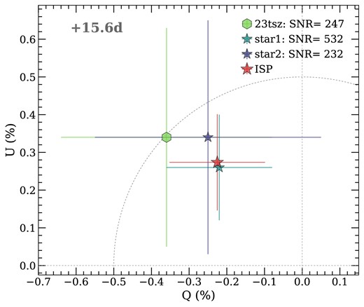
The Stokes Q–U diagram of the V-band polarimetry, before ISP correction, taken at |$+15.6\, \mathrm{ d}$|. The measured polarization fraction of SN 2023tsz is consistent with the two other stars present in the image. After correcting for the Galactic ISP and polarization bias, we find |$P=0.08\pm 0.31$| per cent. |$Q=0$| per cent and |$P=1$| per cent have been marked with dotted lines.
Whilst we cannot directly estimate the host galaxy ISP, its maximum value should be related to the host galaxy extinction via the following empirical relation: |$P_{\mathrm{ISP}} \lt 9 \times E (B-V)$| (Serkowski, Mathewson & Ford 1975). The photometric and spectroscopic properties of the SN and the host galaxy properties all support the assumption of low host extinction, implying that the host ISP should also be low. As such, we can conclude that the polarization of SN 2023tsz is likely intrinsically low. The V band covers mostly continuum and the only clear line feature in the V bandpass is He i 5876 Å and that manifests mostly as emission. Line emission is inherently unpolarized, so it can only decrease the observed V-band polarization, but as the line is narrow (|$2.25^{+0.73}_{-0.21}\times 10^{3}$| km s−1) and covers only a small part of the whole band, the depolarizing effect should be negligible. As such, we assume the low polarization is that of the continuum and conclude that the SN photosphere was consistent with spherical symmetry at |$+15.64$| d post-peak.
3.4 Host data
We fit the photometric data for the host of SN 2023tsz using the cigale software (Boquien et al. 2019). cigale works by computing composite spectral energy distribution (SED) models of the galaxy using specified modules that each deal with a different component of a galaxy’s emission. It then fits these models to the input observations, which for the host of SN 2023tsz are the survey observations detailed in Table A2, and determines the best-fitting model, the one with the lowest reduced |$\chi ^{2}$|. Each module has multiple parameters, and the user provides an array of values for each of them. cigale then computes a model for each combination of parameter values. Galaxy templates were generated using a delayed star formation history (SFH), using the simple stellar population models of BC03 (Bruzual & Charlot 2003). Dust attenuation was included using the Calzetti et al. (2000) law and dust emission following the Draine & Li (2007) templates.
To allow us to compare how the age of the burst affects the other parameters in the SED fitting, three different burst age parametrizations were tested: the first had the age of the burst allowed over a range of ages from 5 to 200 Myr (scenario 1), the second over a range of ages from 100 to 500 Myr (scenario 2), and the third from 1 to 5 Myr (scenario 3). The 5–200 Myr range provided the best fit, with a burst age of 50 Myr. The best-fitting model SED, from scenario 1, is shown in Fig. 9. The key parameters of the best fit in each scenario are shown in Table 3. As can be seen, all the fits have comparable values for their SFR, stellar mass, and specific SFR (sSFR) meaning the best-fitting values are robust. For the rest of the analysis, we use the best fit from scenario 1 and its values for SFR, |$2.64\times 10^{-3}$| |${\rm M}_{\odot } \, {\rm yr}^{-1}$|, stellar mass, |$1.15\times 10^{7}$| |${\rm M}_{\odot }$|, and sSFR, |$2.29\times 10^{-10}$| |${\rm yr}^{-1}$|. These values are shown in comparison to a sample of stripped-envelope (SE) SN host galaxies, from Schulze et al. (2021), in Fig. 10.
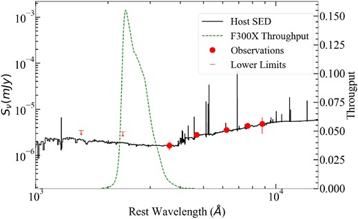
The best-fitting SED of the host of SN 2023tsz from cigale is shown by the solid line. The observations from KiDs and VIKING are shown by the data points. The dashed line indicates the region (bandpass and throughput) of the spectrum that would have been observed by the HST F300X filter had the host been at the redshift of PS1-12sk (|$z=0.054$|).
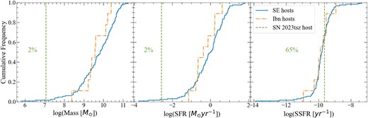
Cumulative frequency plots showing the stellar mass (left), SFR (centre), and sSFR (right) of the host of SN 2023tsz (dashed line), SN Ibn hosts (9; dash–dot line), and SE SN hosts (9 SN Ibn and 118 SN Ib/c; solid line). The host properties are from Schulze et al. (2021). The percentage of supernovae hosts with a mass (left), SFR (centre), or sSFR (right) less than the host of SN 2023tsz is indicated in each plot.
Key parameters of different SED fits to the host of SN 2023tsz, with different SFH burst age parametrizations. The chosen burst age for the best fit (i.e. the lowest reduced chi-squared) is given with the model.
| Model | log(SFR) (|${\rm M}_{\odot } \, {\rm yr}^{-1}$|) | log(stellar mass) (|${\rm M}_{\odot }$|) | log(sSFR) (|${\rm yr}^{-1}$|) | |$\chi ^2$| |
|---|---|---|---|---|
| Scenario 1 (burst age = 50 Myr) | –2.58 | 7.06 | –9.64 | 0.22 |
| Scenario 2 (burst age = 100 Myr) | –2.83 | 7.08 | –9.91 | 0.44 |
| Scenario 3 (burst age = 5 Myr) | –2.95 | 6.64 | –9.59 | 1.74 |
We measure the galaxy to have a radius of 1.6 arcsec, equivalent to a physical radius of 1.0 kpc, defined by the radius encompassing 99 per cent of the galaxy’s light in the Legacy Survey DR9 g-band images. This equates to an area of 8.2 arcsec2 and a physical size of 3.1 kpc2. This radius is shown in Fig. 1. This, along with the SFR from our best-fitting SED, puts the SFR density of SN 2023tsz’s host at |$9.3 \times 10^{-4} \, {\rm M}_{\odot } \, {\rm yr}^{-1} \, {\rm kpc}^{-2}$|. When we compare this to the combined data sets of Hosseinzadeh et al. (2019) and Galbany et al. (2018) there are only two SN Ib/c (4.4 per cent of the sample) and one SN Ibn (5.9 per cent of the sample) host galaxies with lower SFR densities.
Using the fraction of stars per unit mass that produce CC SNe from Botticella et al. (2012), |$K_{\mathrm{CC}} \sim 0.01 \, {\rm M}_{\odot }^{-1}$|, the SFR from our best-fitting SED would mean that we expect a massive star to explode in this galaxy every |${\approx}35 \, {\rm kyr}$|. As SNe Ibn account for |${\approx} 1 {{\, \rm per\, cent}}$| of CC SNe (Maeda & Moriya 2022), we would expect to observe an event such as SN 2023tsz in its host approximately once in every 3.5 Myr. This expectation could still be too frequent given that lower mass star-forming regions, as expected in such a low star formation host, may underproduce the most massive stars owing to stochastic initial mass function sampling (Stanway & Eldridge 2023).
The only other SN Ibn that was discovered in a low SFR region is PS1-12sk (Sanders et al. 2013). No host was found at PS1-12sk’s location in the Hubble Space Telescope (HST) observations (Hosseinzadeh et al. 2019). We simulated an observation of the host of SN 2023tsz at the redshift of PS1-12sk to investigate if it would have been visible in the HST observations. This simulated observation was done using the pysynphot package (STScI Development Team 2013) into which we input the SED generated using cigale. The part of the SED is visible in the HST F300X filter at |$z = 0.054$|, the redshift of PS1-12sk, is shown in Fig. 9. We obtained an apparent magnitude of 24.61 mag for the simulated observation, equating to a surface brightness of 26.90 mag arcsec−2. This surface brightness is higher than the |$5\sigma$| limit, 27.5 mag arcsec−1 measured by Hosseinzadeh et al. (2019) meaning a host comparable to the host of SN 2023tsz would have just been visible in their observations.
4 DISCUSSION
4.1 Comparison of explosion parameters to other SN Ibn/Icn
The decline rate and peak magnitude of SN 2023tsz are comparable to the population of SNe Ibn (Fig. 3). When comparing the parameters from fitting the CSM + Ni model to the bolometric light curve of SN 2023tsz with those of other SNe Ibn (Pellegrino et al. 2022a) and SNe Icn (Pellegrino et al. 2022b) using the same models, we find that our ejecta mass |$M_{\rm ej} = 0.59^{+0.69}_{-0.38} \, {\rm M}_{\odot }$| is comparable to their values when considering their associated uncertainties. Our value for the CSM mass |$M_{\rm CSM} = 0.05^{+0.05}_{-0.02} \, {\rm M}_{\odot }$| is lower than that found for other SN Ibn fit using the same models with the exception of SN 2019wep, which had a comparable value when considering the associated errors. SN 2023tsz is on the upper end for decline rates of SN Ibn, so this lower value of |$M_\mathrm{{CSM}}$| is expected. The large uncertainties on our value of |$M_\mathrm{ej}$| are most likely due to our limited photometric coverage of the rise and peak phases, meaning our model fitting is not well constrained at those epochs. The inferred |$^{56} {\rm Ni}$| mass is higher than those found for the other SNe Ibn fit using the same model. We take our value for the |$^{56} {\rm Ni}$| produced as an upper limit, as our final photometric observation lies below our model fit, which means it is consistent with the lower |$^{56} {\rm Ni}$| derived for other SNe Ibn. The final photometric data point lying below the model could indicate incomplete trapping of the |$\gamma$|-rays from the decay of |$^{56} {\rm Ni}$| (Clocchiatti & Wheeler 1997). We were unable to obtain later photometry to help further constrain the |$M_\mathrm{{Ni}}$| due to SN 2023tsz becoming too faint for our instruments. In summary, the key parameters (Ni, CSM, and ejecta masses) of SN 2023tsz show general agreement with those of other SNe Ibn when considering associated uncertainties.
4.2 Spherical symmetry in SNe Ib/cn
The polarimetry of SN 2023tsz is an important addition to the sample of three other SNe Ibn/Icn with polarimetric observations. The polarization factor of SN 2023tsz, |$P=0.08\pm 0.31 \, {\rm per \, cent}$|, is consistent with it having spherically symmetric photosphere at |$+15.64$| d post-peak. This observed spherically symmetric photosphere does not rule out a progenitor binary system, as at the time of observation the photosphere will have engulfed the binary system. To date, there are only three other SNe Ibn/Icn with conclusive polarimetry. SN Ibn 2023emq (Pursiainen et al. 2023b) and SN Icn 2021csp (Perley et al. 2022) exhibited low polarization, while SN Ibn 2015G showed polarization up to |${\approx} 2.7 \, {\rm per \, cent}$|, but the exact value is unclear due to an uncertain, but possibly substantial, ISP contribution (Shivvers et al. 2017). While the sample is still small, most SNe Ibn/Icn appear to be consistent with a high degree of spherical symmetry, but at most one appears to have possibly exhibited an aspherical photosphere. Further polarimetry of SNe Ibn/Icn will be needed to either confirm whether this one possible aspherical case is an outlier among a generally spherically symmetric population or if there is a population of aspherical interacting SNe.
4.3 Causes of asymmetric line profiles
The blue asymmetry seen in SN 2023tsz’s |$+70.2$| d post-peak spectrum could potentially be explained by a number of scenarios. One scenario is dust formation within the SN ejecta. Dust can partly absorb light from the far side of the ejecta, suppressing the redshifted part of the emission lines. This effect has been observed in some Type II SNe, such as SN 1987A and SN 1999em (Lucy et al. 1989; Elmhamdi et al. 2003) more than a year after explosion. It typically only appears at later times as the ejecta need to cool below the threshold for dust formation. At the epoch of the spectrum, we infer a blackbody temperature of |$T_{\mathrm{BB}}\gt 9000 \, {\rm K}$| which is inconsistent with dust formation in the ejecta. However, given the low ejecta mass, it is possible that SN 2023tsz quickly transitioned from the photospheric phase to the nebular phase. If this is the case then the blackbody approximation no longer holds. The excess flux below 5500 Å seen in the +36.3 d spectrum, which is seen in other interacting SN at comparable times (Perley et al. 2022), and is similar to the forest of iron lines found in modelling the nebular phase of SE SNe (Dessart et al. 2023), suggests this could be the case. As our temperature fitting is heavily dependent on our g-band observations, the excess flux in this region could lead to a higher fitted temperature that is actually the case. If indeed the temperature is lower than that of our blackbody fit, then dust formation could have occurred. Dust formation has been observed in SN 2006jc and OGLE-2012-SN-006 at a similar epoch to our observation (Mattila et al. 2008; Gan, Wang & Liang 2021). These objects had near-infrared (NIR) observations that showed a second blackbody component that was consistent with thermal radiation from newly formed dust. As we lack NIR observations, we cannot investigate whether this is the case in SN 2023tsz to confirm dust formation as a cause of the line asymmetry.
Another possibility is that the unshocked CSM is causing the blue asymmetry. If there is CSM in the line of sight, it will scatter the photons from the receding ejecta (relative to our line of sight) more than the approaching ejecta, leading to the observed blue-dominant asymmetry. A visual representation of this is given in Taddia et al. (2020). Based on our polarimetric observation, the photosphere of SN 2023tsz is consistent with spherical symmetry, which implies a large fraction of the CSM likely follows a spherical distribution, as expected of a WR star wind. This directly means that there should be CSM in the line of sight, making this scenario a possibility. However, unlike in Taddia et al. (2020), the asymmetry in SN 2023tsz occurs after we see the broadening of the narrow-line features, caused by the receding of the photosphere revealing the shocked CSM. If the asymmetry was due to the absorption of the emission from the receding shocked CSM, then it should have occurred with the broadening of the lines.
It is also possible that the ejecta were asymmetric, but appeared to be symmetric at +15.6 d because the asymmetric region was within the photosphere. At +70.2 d the photosphere could have receded and revealed this asymmetric ejecta, producing asymmetric lines. Without polarimetry at the same epoch, we cannot rule out this possibility solely on our earlier observation of symmetry. However, without such observations, we also cannot confirm it.
4.4 Implications for SN Ibn progenitors and hosts
The characterization study of Pastorello et al. (2015b) found that, at the time, all but one SNe Ibn were found in spiral galaxies. As they were typically found in star-forming regions this supported the idea that their progenitors are massive stars. However, the one exception was PS1-12sk (Sanders et al. 2013). As PS1-12sk was found in a region with a low SFR it brought into question whether all SNe Ibn come from massive stars, and if not, then what is the mechanism that strips their progenitors?
SN 2023tsz is now the second SN Ibn that has been discovered in a low SFR region comparable to PS1-12sk, although, unlike PS1-12sk, SN 2023tsz has a visible host. If SN 2023tsz and PS1-12sk both come from non-massive star progenitors, then it could suggest that alternate channels for SNe Ibn are more common than initially thought. However, a low SFR does not rule out a massive star progenitor. The work by Hosseinzadeh et al. (2019) focused solely on examining the SFR, excluding the sSFR due to the limitations of their HST observations. The sSFR is a better indicator of the current star formation of a galaxy than SFR alone, because sSFR reveals how efficiently the galaxy is forming stars relative to its mass. The sSFR of the host of SN 2023tsz is in the 65th percentile for the hosts of SE SN, as shown in Fig. 10. This is not unexpected as lower mass galaxies are observed to have higher sSFR than higher mass galaxies at low redshifts (Bauer et al. 2013; Geha et al. 2024). Based on the sSFR alone we cannot rule out a massive star progenitor. This is further supported by lower mass galaxies forming the majority of their stars later than in more massive galaxies (Cowie et al. 1996; Cimatti, Daddi & Renzini 2006; Thomas et al. 2019; Bellstedt et al. 2020).
Estimating the stellar metallicity of the host of SN 2023tsz using a galaxy mass–metallicity relation (MZR) derived from the observationally supported simulations of Ma et al. (2016) gives |$\log (Z_{*}/{\rm Z}_{\odot })$||$\approx -1.6$|. The galaxies of comparable mass used to derive the MZR come from Kirby et al. (2013), and have a range of stellar metallicities from |$-1.3$| to |$-1.7$|. For single stars, wind-driven stripping is weaker at lower metallicity, making it inefficient at producing WRs (Mokiem et al. 2007), although rotation of the star can help in this regard (Meynet & Maeder 2005). At these low metallicities, binary interactions are thought to be the dominant envelope stripping mechanism (e.g. Bartzakos, Moffat & Niemela 2001), although more recent work suggests that this may not necessarily be the case (Shenar et al. 2020). The binary fraction of WR stars appears to be independent of metallicity down to the metallicities of the Magellanic Clouds (Foellmi, Moffat & Guerrero 2003). However, the inferred metallicity of the host of SN 2023tsz is a factor |${\sim}10$| lower than that of the Small Magellanic Cloud. Observational constraints on populations at these metallicities from Local Group dwarfs are extremely difficult. The work of Foellmi et al. (2003) is based on only 12 sources, but it does suggest that WR stars are not ruled out as progenitors in these low-mass hosts, and consequently cannot be ruled out as a progenitor for SN 2023tsz.
Our simulated observation shows that the host of SN 2023tsz would have just been visible in the observations of the region of PS1-12sk (Hosseinzadeh et al. 2019). However, we note that SE SNe have been discovered in hosts an order of magnitude less massive (Schulze et al. 2021) than that of SN 2023tsz. Such a galaxy would plausibly not have been observable in the observations of Hosseinzadeh et al. (2019). We further note the similarity in larger scale environment between SN 2023tsz and PS1-12sk: in the outskirts of a more massive local galaxy. Although the satellite nature of the host of SN 2023tsz is uncertain, such a location is to be expected of faint, low-mass satellite galaxies. Given the low luminosity of these galaxies it is possible that SNe in such hosts at higher redshifts may be misattributed to being highly offset from a more massive galaxy.
The exceptional nature of the host of SN 2023tsz then highlights a need for a thorough investigation of the host environments of SNe Ibn. It is not yet clear if they are over-represented in low-mass, low-metallicity galaxies compared to other CC SN types. Any such preference would require explanation by purported progenitor systems. If a population of SNe Ibn exists in low-mass host galaxies, it becomes important to determine whether SNe Ibn from more actively star-forming regions share the same progenitor scenario. Alternatively, the SNe Ibn population may consist of two separate progenitor groups that give rise to SNe with the same observed properties.
5 CONCLUSION
We have presented the analysis of the photometric, spectroscopic, polarimetric, and host properties of SN 2023tsz, a typical SN Ibn that stands out due to its association with an exceptionally low-mass host galaxy. This study adds to the limited sample of SN Ibn with polarimetric data, making it only the fourth such SN Ib/cn to be studied in this way. It is also the first SN Ibn to be discovered, reported, and classified entirely by the GOTO collaboration. The key findings of our analysis are summarized below.
The peak absolute magnitude of SN 2023tsz, |$M_{r} = -19.72 \pm 0.04$| mag, and its decline rate of |$0.145 \pm 0.002$| mag d−1 are consistent with other known SNe Ibn, indicating it is a typical member of the class.
Our modelling of the bolometric light curve using a CSM + Ni model resulted in inferred values of |$M_{\mathrm{CSM}} = 0.05^{+0.05}_{-0.02} \, {\rm M}_{\odot }$|, |$M_{\mathrm{ej}} = 0.59^{+0.69}_{-0.38} \, {\rm M}_{\odot }$|, and |$M_{\mathrm{Ni}} = 0.04^{+0.01}_{-0.01} \, {\rm M}_{\odot }$|, all of which are comparable to other SN Ibn. The high initial decline rate of SN 2023tsz, compared to other SNe Ibn, is consistent with it having a low CSM mass.
At later times, the spectrum of SN 2023tsz showed blue asymmetry in its prominent emission lines. While the exact cause is uncertain we suggest three plausible explanations. The first explanation is dust formation in a cool dense shell could absorb emission from the receding ejecta. Whilst our temperature fitting does not rule this scenario out we cannot confirm it without contemporaneous NIR and mid-infrared data. A second explanation involves the scattering of redshifted photons by CSM, however, the asymmetry appears later than we would expect for this explanation. The third is that we are seeing asymmetric ejecta that were, at the time, below the earlier observed symmetric photosphere. However, this cannot be confirmed without coeval polarimetry.
Polarimetric observations showed a polarization fraction of |$P=0.08 \pm 0.32$| per cent at 15.6 d post-peak, suggesting a symmetric photosphere. This is consistent with three of the four polarimetric observations of SNe Ib/Icn to date.
From our SED fitting, the host galaxy of SN 2023tsz has SFR of |$2.64 \times 10^{-3} \, {\rm M}_{\odot } \, {\rm yr}^{-1}$|, a stellar mass of |$1.15 \times 10^{7} \, {\rm M}_{\odot }$|, and a sSFR of |$2.29 \times 10^{-10} \, {\rm yr}^{-1}$|. While its SFR and stellar mass are in the 2nd percentile for SE SN hosts, its sSFR is in the 65th percentile (Schulze et al. 2021).
We estimate a host metallicity of log(|$Z_{*}/{\rm Z}_{\odot }$|) |$\approx -1.6$| based on the MZR, indicating that the progenitor system of SN 2023tsz is from an extremely low-metallicity environment.
These findings show that SNe Ibn can occur in extraordinarily low-mass and low-metallicity galaxies. This environment poses problems for the stellar evolution of a single-stripped star progenitor, although does not rule them out. An important question that remains surrounding SNe Ibn: Are they over-represented in these low-mass galaxies, and if so, why? These host galaxies are often too faint to be detected by contemporary sky surveys, potentially skewing our understanding of the host environments of SNe Ibn.
The host of SN 2023tsz shows the need for further investigation into the occurrence rates of SNe Ibn in such hosts. Any over-representation in low-mass, low-metallicity hosts will need to be addressed in future proposed progenitor scenarios.
ACKNOWLEDGEMENTS
BW acknowledges the UK Research and Innovation's (UKRI) Science and Technology Facilities Council (STFC) studentship grant funding, project reference ST/X508871/1.
The authors would like to acknowledge the University of Warwick Research Technology Platform (SCRTP) for assistance in the research described in this paper.
This work used observations from the Las Cumbres Observatory Global Telescope Network. Time on the Las Cumbres Observatory network was provided via the Optical Infrared Co-ordination Network for Astronomy (OPTICON, proposal 23B030).
JL, MP, and DO acknowledge support from a UKRI Fellowship (MR/T020784/1).
DLC acknowledges support from the STFC, grant number ST/X001121/1.
TLK acknowledges support via a Research Council of Finland grant (340613; PI: R. Kotak), and from the STFC, grant number ST/T506503/1).
For the purpose of open access, the author has applied a Creative Commons Attribution (CC BY) licence to the Author Accepted Manuscript version arising from this submission.
SM was funded by the Research Council of Finland project 350458.
LK and LKN thank the UKRI Future Leaders Fellowship for support through the grant MR/T01881X/1.
Based in part on observations made with the Nordic Optical Telescope, owned in collaboration by the University of Turku and Aarhus University, and operated jointly by Aarhus University, the University of Turku, and the University of Oslo, representing Denmark, Finland, and Norway, the University of Iceland and Stockholm University at the Observatorio del Roque de los Muchachos, La Palma, Spain, of the Instituto de Astrofisica de Canarias. The NOT data presented here were obtained with ALFOSC, which is provided by the Instituto de Astrofisica de Andalucia (IAA) under a joint agreement with the University of Copenhagen and NOT.
The Gravitational-wave Optical Transient Observer (GOTO) project acknowledges the support of the Monash-Warwick Alliance, University of Warwick, Monash University, University of Sheffield, University of Leicester, Armagh Observatory & Planetarium, the National Astronomical Research Institute of Thailand (NARIT), Instituto de Astrofísica de Canarias (IAC), University of Portsmouth, University of Turku, and the STFC (grant numbers ST/T007184/1, ST/T003103/1, and ST/Z000165/1).
DS acknowledges support from the STFC via grant numbers ST/T003103/1, ST/Z000165/1, and ST/X001121/1.
JPA’s work was funded by the National Agency for Research and Development (ANID), Millennium Science Initiative, ICN12_009.
TP acknowledges the financial support from the Slovenian Research Agency (grants I0-0033, P1-0031, J1-8136, J1-2460, and Z1-1853).
PC was supported by the STFC (grants ST/S000550/1 and ST/W001225/1).
RS was funded by a Leverhulme Research Project Grant.
MJD was funded by the STFC as part of the GOTO project (grant number ST/V000853/1).
MRM acknowledges a Warwick Astrophysics prize post-doctoral fellowship made possible thanks to a generous philanthropic donation
AS acknowledges the Warwick Astrophysics PhD prize scholarship made possible thanks to a generous philanthropic donation.
Based on observations collected at the European Organisation for Astronomical Research in the Southern Hemisphere, Chile, as part of ePESSTO+ (the advanced Public ESO Spectroscopic Survey for Transient Objects Survey). ePESSTO+ observations were obtained under ESO program ID 112.25JQ.
AA acknowledges the Yushan Fellow Program by the Ministry of Education, Taiwan for the financial support (MOE-111-YSFMS-0008-001-P1).
This research has made use of data obtained from the High Energy Astrophysics Science Archive Research Center (HEASARC) and the Leicester Database and Archive Service (LEDAS), provided by NASA’s Goddard Space Flight Center and the School of Physics and Astronomy, University of Leicester, UK, respectively.
LG, TEM-B, and CPG acknowledge financial support from AGAUR, CSIC, MCIN, and AEI10.13039/501100011033 under projects PID2023-151307NB-I00, PIE 20215AT016, CEX2020-001058-M, FJC2021-047124-I, 2021-BP-00168, and 2021-SGR-01270.
MN was supported by the European Research Council (ERC) under the European Union’s Horizon 2020 Framework Programme (grant agreement no. 948381) and by UK Space Agency grant no. ST/Y000692/1.
TWC acknowledges the Yushan Fellow Program by the Ministry of Education, Taiwan for the financial support (MOE-111-YSFMS-0008-001-P1).
PO was supported by the STFC (grant number ST/W000857/1).
RK acknowledges support from the Research Council of Finland (grant no. 340613).
HK was funded by the Research Council of Finland projects 324504, 328898, and 353019.
We would like to thank the anonymous reviewer for their helpful comments and feedback.
DATA AVAILABILITY
The underlying raw photometric, spectroscopic, and polarimetric data are available from the relevant data archives. The analysed data will be shared on reasonable request to the corresponding author.
Footnotes
Based on a Transient Name Server, https://www.wis-tns.org/, query on 2024 June 18.
github.com/jkrogager/PyNOT/
REFERENCES
APPENDIX A: TABLES
Spectroscopic time series of SN 2023tsz.
| Date | MJD | Phase (d) | Telescope | Instrument | Grism | R (|$\lambda /\Delta \lambda$|) | Range (Å) |
|---|---|---|---|---|---|---|---|
| 2023-09-28 | 60216.23 | +4.2 | NOT | ALFOSC | Gr4 | 360 | 3200–9600 |
| 2023-10-20 | 60237.95 | +25.9 | HCT | HFOSC | Gr7/Gr8 | 500 | 3800–9250 |
| 2023-10-30 | 60248.28 | +36.3 | NTT | EFOSC2 | Gr13 | 355 | 3685–9315 |
| 2023-12-03 | 60282.19 | +70.2 | GTC | OSIRIS+ | R1000B+R1000R | 1018, 1122 | 3630–10000 |
Survey data of the host of SN 2023tsz.
| Filter | Mag | Error | Survey |
|---|---|---|---|
| z | 22.20 | 0.34 | VIKING |
| g | 22.79 | 0.05 | KiDS |
| i | 22.31 | 0.07 | KiDS |
| r | 22.53 | 0.04 | KiDS |
| u | 23.37 | 0.20 | KiDS |
| Filter | Mag | Error | Survey |
|---|---|---|---|
| z | 22.20 | 0.34 | VIKING |
| g | 22.79 | 0.05 | KiDS |
| i | 22.31 | 0.07 | KiDS |
| r | 22.53 | 0.04 | KiDS |
| u | 23.37 | 0.20 | KiDS |
