


ABSTRACT
The AU Microscopii planetary system is only 24 Myr old, and its geometry may provide clues about the early dynamical history of planetary systems. Here, we present the first measurement of the Rossiter–McLaughlin effect for the warm sub-Neptune AU Mic c, using two transits observed simultaneously with the European Southern Observatory's (ESO's) Very Large Telescope (VLT)/Echelle SPectrograph for Rocky Exoplanets and Stable Spectroscopic Observations (ESPRESSO), CHaracterising ExOPlanet Satellite (CHEOPS), and Next-Generation Transit Survey (NGTS). After correcting for flares and for the magnetic activity of the host star, and accounting for transit-timing variations, we find the sky-projected spin–orbit angle of planet c to be in the range |$\lambda _{\mathrm{c}}=67.8_{-49.0}^{+31.7}$| degrees (1|$\sigma$|). We examine the possibility that planet c is misaligned with respect to the orbit of the inner planet b (|$\lambda _{\mathrm{b}}=-2.96_{-10.30}^{+10.44}$|), and the equatorial plane of the host star, and discuss scenarios that could explain both this and the planet’s high density, including secular interactions with other bodies in the system or a giant impact. We note that a significantly misaligned orbit for planet c is in some degree of tension with the dynamical stability of the system, and with the fact that we see both planets in transit, though these arguments alone do not preclude such an orbit. Further observations would be highly desirable to constrain the spin–orbit angle of planet c more precisely.
1 INTRODUCTION
Transiting planets around young stars are useful laboratories for studying the formation and evolution of planetary systems. This is particularly true for systems younger than 100 Myr. At such young ages, the key processes shaping the final system are at their strongest, including interactions between the planets, the disc they form in, and the host star (Burrows et al. 1997; Mordasini et al. 2012; Owen 2019). In particular, information about the early dynamical history of the system is encoded in the orientation of the orbits of young planets and the spin of the host star (Winn & Fabrycky 2015). Planets might undergo scattering events, collisions (i.e. giant impacts), or secular perturbations after their formation within the protoplanetary disc, which can lift their orbital inclinations (Wu & Murray 2003; Chatterjee et al. 2008). Subsequently, the orbital plane might be altered by tidal dissipation (see e.g. Bolmont & Mathis 2016). Obliquity measurements for young planets with well-measured ages are vital to constrain the key time-scales for these mechanisms. Specifically, measurements for systems that are too young to have undergone significant tidal alteration of obliquity allow us to gain insight into their initial configurations (Mantovan et al. 2024). However, these measurements are still scarce. Only seven such measurements have been published to date (see Albrecht, Dawson & Winn 2022, for a review). Some practical obstacles to performing these measurements are the rapid rotation and intense magnetic activity of the host stars, which severely hamper the detection and characterization of young planets.
The AU Microscopii system illustrates these points. It is one of the most interesting young multiplanet systems known to exist, and is seemingly favourable for observations because it is only 9.7 pc away (Gaia Collaboration 2018) and is one of the brightest M dwarfs in the sky (|$V=8.7$|; Torres et al. 2006). As a member of the Beta Pictoris moving group (Barrado y Navascués et al. 1999), it has a well-constrained age of |$24.3_{-0.3}^{+0.3}$| Myr (e.g. Malo et al. 2014; Mamajek & Bell 2014; Messina et al. 2016; Miret-Roig et al. 2020; Galindo-Guil et al. 2022) and has long been known to host an edge-on debris disc (Kalas, Liu & Matthews 2004), in which fast-moving structures of unclear origin have been imaged with Spectro-Polarimetic High contrast imager for Exoplanets REsearch (SPHERE) on the Very Large Telescope (VLT) and Hubble Space Telescope (HST; Boccaletti et al. 2015, 2018). However, the star’s brightness and radial velocity (RV) have been intensively monitored and found to be highly variable and complex. The light curve displays quasi-periodic brightness fluctuations that indicate a 4.85-d rotation period (Rodono et al. 1986; Hebb et al. 2007), along with frequent flares (Robinson et al. 2001). The spin of the star appears to be closely aligned with the debris disc, based on the comparison between the inclinations of the stellar rotation axis, |$i_{\rm {star}}=87.3^{+1.9}_{-2.8}$| degrees, and the disc axis, |$i_{\rm {disc}}=89.4^{+0.1}_{-0.1}$| degrees (Hurt & MacGregor2023).
Two close-in transiting Neptune-sized planets were discovered around AU Mic using photometry from the Transiting Exoplanet Survey Satellite (TESS; Ricker et al. 2015). The planets were reported by Plavchan et al. (2020) and Martioli et al. (2021) with orbital periods of |$P_{\mathrm{b}}=8.46$| d and |$P_{\mathrm{c}}=18.86$| d, respectively. Ongoing monitoring of the transits using the TESS, Spitzer (Werner et al. 2004), and CHaracterising ExOPlanet Satellite (CHEOPS; Benz et al. 2021) space telescopes, and ground-based observatories, revealed significant transit-timing variations (TTVs) in the system (Szabó et al. 2021, 2022; Wittrock et al. 2022, 2023). To explain the observed TTVs, Wittrock et al. (2023) invoked an additional, non-transiting planet ‘d’ located between planets b and c, with a mass comparable to the Earth and an orbital period of |$P_\mathrm{ d}=12.73$| d. Several studies have reported masses for the two transiting planets based on optical and near-infrared RV monitoring (Cale et al. 2021; Zicher et al. 2022; Donati et al. 2023). The star’s rapid rotation and strong magnetic activity induce RV variations that can reach up to 1 km s−1 in amplitude, dwarfing the planet-induced signals and making the resulting mass measurements highly dependent on the modelling of stellar activity. In this work, we adopt the mass and radius estimates from Donati et al. (2023) of |$R_{\mathrm{b}}=3.55\pm 0.13\, \mathrm{R}_{\oplus }$|, |$M_{\mathrm{b}}=10.2^{+3.9}_{-2.7}\, M_{{\oplus }}$|, |$R_{\mathrm{c}}=2.56\pm 0.12\, \mathrm{R}_{\oplus }$|, and |$M_{\mathrm{c}}=14.2^{+4.8}_{-3.5}\, \mathrm{M}_{\oplus }$|. Donati et al. (2023) did not confirm or rule out planet d, but reported an additional candidate non-transiting planet with a period of |$P_\mathrm{ e}=33.4$| d and a mass of |${\sim} 35\, \mathrm{M}_{\oplus }$|, which may also play a role in explaining the observed TTVs.
The fact that planet c is denser than planet b (|$\rho _{\mathrm{b}}=1.26_{-0.43}^{+0.68} \mathrm{~g} \mathrm{~cm}^{-3}$|, |$\rho _{\mathrm{c}}=4.7_{-1.6}^{+2.5} \mathrm{~g} \mathrm{~cm}^{-3}$|; Donati et al. 2023) suggests that planet c has a more massive solid core and a smaller H/He gaseous envelope (Zicher et al. 2022). This can be in tension with the general theoretical expectation that a more massive solid core should be able to accrete a larger mass of gas from the protoplanetary disc (Owen & Wu 2013). Possible explanations include (a) planet c could be the result of a giant impact between two outer planets in the system, or (b) planets b and c could have formed in starkly different conditions within the same disc (Zicher et al. 2022). Measuring the orientation of AU Mic c’s orbit might be helpful to differentiate between these scenarios.
When a transiting planet crosses over the disc of the host star, a portion of the blueshifted or redshifted starlight (due to stellar rotation) is blocked from the line of sight. This causes distortions of the disc-integrated stellar spectrum and an ‘anomalous’ apparent RV, which reflects the trajectory of the planet. This is the so-called Rossiter–McLaughlin (RM) effect, which allows for the measurement of the projected angle between the planet’s orbit and the stellar rotation axis, also known as the projected spin–orbit angle (Queloz et al. 2000; Winn et al. 2005). Multiple studies (Hirano et al. 2020; Palle et al. 2020; Addison et al. 2021; Martioli et al. 2021) have used RM observations to constrain the projected spin–orbit angle of AU Mic b to be consistent with zero (|$\lambda _{\mathrm{b}}=-2.96_{-10.30}^{+10.44}$|; Palle et al. 2020). In this work we aim to make the first same type of measurement for planet c. A misaligned orbit for planet c would suggest that the planet has undergone significant dynamical interactions after the dispersal of the gas disc, thus favouring the giant-impact scenario (a), or other type of dynamical disruption. In contrast, an aligned orbit would indicate a more sedate dynamical history, compatible with scenario (b).
The measurement of the projected spin–orbit angle |$\lambda$| from RM observations is known to be affected by significant degeneracies with other parameters that are also related to the local RV of the star along the transit chord. These include the time of the mid-point of the transit, the planetary orbital inclination i (or impact parameter, |$b=a \cos i /R_\star$|), and the star’s projected rotation velocity |$v \sin i_\star$| (e.g. Gaudi & Winn 2007). Thanks to the wealth of existing space-based photometry and high-resolution spectroscopy, most of these parameters are relatively well known for AU Mic and its transiting planets (e.g. |$P_{\rm rot}=4.856\pm 0.003$| d and |$v \sin i_\star = 8.5\pm 0.2$| km s−1; Donati et al. 2023). However, both planets display TTVs, with TTV amplitudes of 20–30 min reported for planet b, and 5–10 min for planet c (Szabó et al. 2021, 2022; Wittrock et al. 2022, 2023). These TTVs make it challenging to predict transit mid-points precisely enough to plan and interpret our new spectroscopic observations; for planet c, the most recent published observations were conducted 2 yr before our Echelle SPectrograph for Rocky Exoplanets and Stable Spectroscopic Observations (ESPRESSO) observations. We therefore arranged for simultaneous photometric observations with CHEOPS and the Next-Generation Transit Survey (NGTS; Wheatley et al. 2018) to constrain the times of the transit mid-points.
In this work, we present the first measurement of the projected spin–orbit angle for the young sub-Neptune AU Mic c, using simultaneous observations with VLT/ESPRESSO, CHEOPS, and NGTS. The remainder of this paper is structured as follows. We present the observations and basic data reduction steps in Section 2, and describe the steps we took to mitigate the impact of flares in Section 3. We then present our joint model of the CHEOPS photometry and ESPRESSO RVs, and the resulting constraints on the obliquity of planet c, in Section 4. We discuss the limitations and potential implications of our results, and outline our key conclusions and future plans, in Section 5.
2 OBSERVATIONS AND DATA REDUCTION
In this section, we present the observations used in this work and the basic data reduction steps.
2.1 CHEOPS photometry
We observed the two transits of AU Mic c that occurred on the nights of 2023 July 7 and 26 (utc) using the CHEOPS space telescope (Benz et al. 2021) simultaneously with the ESPRESSO observations, in order to refine the mid-transit times and characterize the photometric variability of the host star. CHEOPS’s payload consists of a 32-cm diameter Ritchey–Chrétien telescope and a single-CCD camera covering the wavelength range 330–1100 nm with a field of view of 0.32 deg|$^2$|. Each transit was covered by a CHEOPS visit1 of AU Mic c, taken as part of the CHEOPS Guaranteed Time Observations (GTO) programme number CH_PR140071, were used in this work (see Table 1).
Log of the CHEOPS photometric observations of AU Mic c used in this work.
| Visit no. | Start date (utc) | End date (utc) | File key | CHEOPS product | Integration time (s) | Number of frames |
|---|---|---|---|---|---|---|
| 1 | 2023-07-07 23:25 | 2023-07-08 14:09 | CH_PR140071_TG000901 | Subarray | |$7 \times 5.0$| | 919 |
| 1 | 2023-07-07 23:25 | 2023-07-08 14:09 | CH_PR140071_TG000901 | Imagettes | 5.0 | 6433 |
| 2 | 2023-07-26 20:08 | 2023-07-27 10:51 | CH_PR140071_TG000602 | Subarray | |$7 \times 5.0$| | 1052 |
| 2 | 2023-07-26 20:08 | 2023-07-27 10:51 | CH_PR140071_TG000602 | Imagettes | 5.0 | 7364 |
Note. CHEOPS observation log. The table lists the time interval of individual observations (time notation follows the ISO-8601 convention), the file key, which can be used to locate the observations in the CHEOPS archive, the type of the photometric product, the integration time, and the total number of frames in each visit.
We extracted light curves using point spread function (PSF) fitting on circular ‘imagettes’ of 30-pixel radius centred on the target using the purpose-built software pipe2 (Szabó et al. 2021, 2022; Brandeker, Patel & Morris 2024), which are downloaded for each 5-s exposure. This approach yields similar photometric precision, but better time sampling than the standard CHEOPS Data Reduction Pipeline (DRP).3 The latter performs instead aperture photometry on |$200 \times 200$|-pixel subarrays of the full detector, which, due to their larger size, must be co-added in batches of seven exposures before downloading. The top panel of Fig. 1 shows the pipe CHEOPS light curve after normalizing each visit to unity. The average uncertainty of each photometric data point in the pipe light curve, corresponding to a 5-s integration, is |${\sim} 400$| ppm.
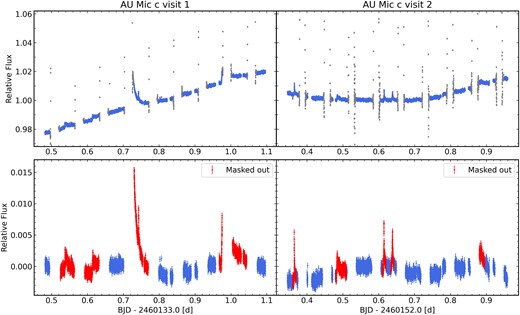
CHEOPS photometric observations of the AU Mic c transits. The left and right columns show the first and second visits, respectively. The top row shows the light curves as extracted by the pipe software after normalizing each visit to unity, with the outliers caused by enhanced stray light at the start and end of each orbit marked in grey. The second row shows the data after subtracting a low-order polynomial trend (for visualization purposes only), with the observations affected by flares highlighted in red.
Outliers are visible just before and after each interruption within a given visit,4 caused by the increased background associated with scattered light from Earth. To remove these outliers, we masked all data taken when the background flux measured by the pipe software exceeded |$20\ \mathrm{electrons\,pixel^{-1}}$|. Outliers identified in this way are marked in grey in the top panel of Fig. 1. This resulted in the removal of 1062 out of 6433 frames (16.5 per cent) for the case of the first visit, and 1592 out of 7364 (21.6 per cent) for the second, leaving a total of 11 143 data points for the remainder of the analysis.
2.2 NGTS photometry
The NGTS is a ground-based photometric facility consisting of 12 independently steerable 0.2-m diameter robotic telescopes, located at the European Southern Observatory (ESO) Paranal Observatory in Chile. AU Mic was observed by NGTS simultaneously with the ESPRESSO observations of the two transits of AU Mic c. The observations were performed using the NGTS multitelescope mode in which multiple NGTS telescopes are used to simultaneously observe the same star. This observing mode has been shown to significantly improve the photometric precision of NGTS data (e.g. Bryant et al. 2020; Smith et al. 2020).
9 telescopes were used on the night of 2023 July 7, and 10 on the night of 2023 July 26. For both nights, the observations were performed using the custom NGTS filter (520–890 nm) and an exposure time of 5 s. The observations were performed with the telescopes heavily defocused in order to avoid saturation and reduce effects of per-pixel sensitivity systematics and X-Y systematics (Southworth et al. 2009a, b; Nascimbeni et al. 2011). A custom aperture photometry pipeline was used to reduce the NGTS data. This pipeline uses the seppython library (Bertin & Arnouts 1996; Barbary 2016) to perform the source and photometry and also utilizes Gaia Data Release 2 information (Gaia Collaboration 2018) to identify comparison stars similar to AU Mic in terms of brightness, colour, and CCD position.
Both nights of observations were severely impacted by clouds, which caused large spurious fluctuations in the photometry (see top row of Fig. B1). The data from the second transit also show ramps at the beginning and end of the night, which are most likely systematic trends due to a lack of insufficient high-quality comparison stars from these observations for such a bright and red star. Even after masking out the most severely affected data (middle row of Fig. B1), the transit signals cannot be easily distinguished from the strong out-of-transit trend and residual short-term systematics. Consequently, the NGTS data were not used in our final analysis, though we did compare them to our fitted model as a consistency check (see Appendix B for details).
2.3 ESPRESSO spectroscopy
We observed two transits of AU Mic c during the nights of 2023 July 7 and 2023 July 26, using the high-precision spectrograph ESPRESSO (Pepe et al. 2014, 2021) mounted on the VLT (Program ID: 111.24VF, PI: H. Yu). For both runs, we used one unit telescope and employed the high-resolution mode (HR; R|$\sim$| 13 800) and the 2x1/SLOW binning/readout mode. Each exposure lasted 300 s. On the first night, 85 spectra were obtained, and on the second night, 66 spectra were obtained, with mean signal-to-noise ratios at 550 nm of 110.2 and 115.3, respectively. During both runs, the airmass ranged between 0.7 and 1.4. During the second run, there was a problem with the control unit of the UT2 telescopes that interrupted the observations at |$\mathrm{BJD}_\mathrm{TDB}=2460152.67160$|. A decision was made to switch telescopes to UT1, and the observations resumed at |$\mathrm{BJD}_\mathrm{TDB}=2460152.73378$|. UT1 was used for the remainder of the night.
The spectra were first reduced using the official ESPRESSO data reduction software (DRS) version 3.0.0 (Pepe et al. 2021). The DRS data products include reduced 2D and 1D (order-merged) spectra as well as cross-correlation functions (CCFs) and RVs extracted by fitting a Gaussian function to each CCF (along with the other parameters of the Gaussian fit). A preliminary inspection of these products revealed that the spectra, CCFs, and RVs were all severely affected by the flares and other stellar activity. We therefore decided to perform our own post-processing and RV extraction, as previous studies (e.g. Bourrier et al. 2021) have shown that this can yield significant gains over the DRS data products.
We used the yarara package (Cretignier et al. 2021) to perform post-processing of the 1D order-merged (S1D) spectra in order to remove or reduce instrumental and telluric signals. As yarara is a data-driven pipeline, it benefits from using as many observations of a given star with a given instrument as possible. We therefore also re-processed the transit of AU Mic b observed in 2019 with ESPRESSO (Program ID: 103.2010, PI: J. Strachan) and published by Palle et al. (2020). This has the added benefit of broadening the range of barycentric Earth RV spanned by the observations, which helps with the telluric correction step of yarara.
Before entering the yarara pipeline, the spectra were continuum-subtracted using the rassine package (Cretignier et al. 2020). Outliers due to cosmic rays or dead pixels were then masked out via sigma clipping and replaced by the time-median value. The spectra were then corrected for contamination by microtelluric lines, as described in Cretignier et al. (2021). The resulting, post-processed S1D spectra were used in the remainder of the analysis.
After combining all the spectra into a single, master spectrum, we used this to construct a list of non-blended absorption lines (Cretignier et al. 2020). The so-called KITCAT line list was used to compute a CCF for each spectrum, which contains in total around 5000 lines, from which RVs were extracted. However, the resulting RVs were severely affected by flares, so we later re-extracted the RVs using only the subset of lines least sensitive to the flares (see Section 3.3).
It is worth noting that the ESPRESSO and NGTS observations were taken simultaneously, and the two telescopes are only a few km apart. The clouds that affected the NGTS observations probably also affected the ESPRESSO spectra. However, we expect clouds to mainly affect the overall light level and not the shape of the spectrum and hence have a negligible impact on the extracted CCFs and RVs.
3 FLARE MITIGATION
Several flares occurred during and around each of the two observed transits of AU Mic c. Together with the longer term trends caused by star-spots, they dominate both the CHEOPS photometry and ESPRESSO RVs. We therefore adopted the following procedure to mitigate their impact on the final analysis.
3.1 Identifying and masking flares in the CHEOPS light curve
The impact of the flares on the CHEOPS light curves is easier to see after subtracting a second-order polynomial fit, intended to represent the long-term trend due to active regions rotating on the stellar surface (see bottom row of Fig. 1).
While it would in principle be possible to model the flares, this would result in a very large number of free parameters: each flare would require a minimum of three parameters (i.e. the occurrence time, amplitude, and decay rate), and there are at least five flares per visit. We therefore opted to mask out the data that were obviously affected by flares before modelling the spot and transit signals. The data points affected by flares were identified by visual inspection, cross-checking against the flare proxy derived from the ESPRESSO spectra (see Section 3.2) whenever the two time series overlap, and are marked in red in Fig. 1. Although the onset of a flare is relatively straightforward to identify, the tail end of a flare is much less well defined, so we opted to exclude data after each flare up to the end of the affected CHEOPS orbit.
3.2 Extracting a flare proxy from the ESPRESSO spectra
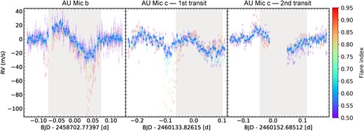
We first characterized the flare signal in the yarara-processed S1D spectra. The flares manifest mainly as emission lines that decay both in width and intensity after the flare impulse on a time-scale of around an hour. We started by selecting two spectra occurring right before and after the start of the largest flare (occurring just before the ingress of the first transit of AU Mic c, on the night of 2023 July 7) and computing the difference between them. We then visually inspected this ‘flare spectrum’ in order to identify atomic line transitions and selected a total of 33 well-defined lines between 4046 and 5434 Å. These lines were cross-matched with values in the National Institute for Standards and Technology (NIST) atomic spectra data base5 to determine their rest wavelengths. The resulting line list was then used to construct a binary mask, which was cross-correlated with each of the observed spectra, after subtracting a reference spectrum. The latter was constructed separately for each season (2021 and 2023), by averaging a small number of spectra taken well away from any flare signals. The resulting ‘flare CCF’ time series for the three visits is shown in the top row of Fig. 2. Each CCF in this time series was fit with a Gaussian function, and the amplitude (or contrast) of this fit – shown in the bottom row of Fig. 2 – constitutes our flare proxy.

Extraction of the flare proxy. The top panel shows the time series of ‘flare CCFs’ (see text for details), from left to right: the 2021 transit of AU Mic b, and then the two transits of AU Mic c observed in 2023. The white markers indicate the mean of a Gaussian fit to each CCF, while their size reflects the amplitude (or contrast of this Gaussian), which is also displayed in the bottom panel, and consists of our flare proxy. The shaded area in each panel in the bottom row indicates the transits of planets b and c. The gap during the second transit of planet c corresponds to the interruption due to the change of the UT telescope.
In this figure, the massive flare that occurred in the middle of the night for visit 1 of AU Mic c is clearly visible. In comparison, this flare was five times larger and twice as long in duration than the ones that occurred for visit 2 or the visit of AU Mic b. Despite our attempts to mitigate it, the flare occurring in this first visit was too strong and made the production of out-of-transit products impossible. It can also be noted that the RVs associated with flares were generally between |$-5$| and 5 km s−1, likely due to the local RV of the surface where they were produced and the extra RV of the ejected matter.
3.3 Extracting flare-resistant CCFs and RVs
The CCFs and RVs produced using the KITCAT mask, shown in red on Fig. 3, are heavily affected by the flares. We therefore sought to identify the subset of lines that are least sensitive to the flares while retaining sufficient RV information content. To quantify the flare sensitivity of each line, we first modelled the time evolution of flux recorded in each pixel (wavelength) of the residual spectrum as the sum of a low-order polynomial (intended to account for spots on the rotating stellar surface) and a term proportional to the flare proxy derived in Section 3.2. We then defined a flare index that quantifies the sensitivity of each line to flares by computing the average of the correlation coefficient over a line profile in a given velocity window of |$\pm$|10 km s|$^{-1}$| that contains most of the Doppler information of a spectral line.
RV time series extracted with progressively fewer flare sensitive lines (from red to blue) for the archival transit of planet b (left) and the two transits of AU Mic c (middle and right). The colour represents the mean flare index of all lines in the line list. Note that the flare just before the first transit of AU Mic c caused such a large RV perturbation in the RVs extracted with all the lines (red points) that it goes beyond the y-axis range shown here. A quadratic RV trend caused by rotational modulation of active regions has been fitted to the out-of-transit data and subtracted prior to plotting. The grey shaded area in each panel indicates the duration of the transit.
We used this coefficient to rank the lines in order of flare sensitivity and computed CCFs and RVs with a progressively lower limiting sensitivity to flares until only the 250 least sensitive lines remained. While using fewer stellar lines decreases the impact of the flares, it increases the photon noise. By examining the transit of AU Mic b, we found that the mask with 2000 lines (out of the total |$\sim$|5000 lines) gave the best trade-off between flare suppression and RV precision. The RVs extracted with this mask, shown in dark blue on Fig. 3, were used in the remainder of the analysis.
The final RVs for the archival transit of planet b are very similar to those reported by Palle et al. (2020), which strengthens our confidence in our reduction and RV extraction methodology. The RV uncertainties are somewhat larger, though, because we are using fewer lines. The flare correction described above is effective for most of the archival and new ESPRESSO observations. However, careful examination of Fig. 3 shows that the impact of the strongest flares on the RVs is not completely corrected when the flare proxy (displayed in the bottom row of Fig. 2) exceeds a value of 3. We therefore excluded the RVs taken at those times from the remainder of our analysis.
4 JOINT MODELLING OF THE PHOTOMETRY AND RVs
We jointly modelled the CHEOPS light curve and the ESPRESSO flare-resistant RVs obtained during both transits of AU Mic c in order to derive constraints on the transit times and the projected orbital obliquity simultaneously, while accounting for the uncertainties arising from the star’s intrinsic variability and instrumental noise.
4.1 The model
For both types of observation (photometry and RVs), our model consists of three components. The first component represents the planetary transits. We used the batman package (Kreidberg 2015) to model the photometric transits, and the arome package (Boué et al. 2013) to model the RM effect in the RVs (this model is optimized for CCF-derived RVs). The transit models used for both transits and both types of observations share the same star and planet parameters, including the sky-projected stellar obliquity (|$\lambda$|), inclination (i), scaled semimajor axis (|$a/R_\mathrm{s}$|), planet-to-star radius ratio (|$R_\mathrm{p}/R_\mathrm{s}$|), and limb-darkening coefficients (|$u_1$| and |$u_2$|).6 To account for possible TTVs, each transit was modelled using a separate mid-transit time (|$T_{\mathrm{c}}$|). We placed uninformative uniform priors on the sky-projected stellar obliquity as well as the mid-transit times, and Gaussian priors on all other orbital parameters based on the best-fitting model from the transit analysis in Wittrock et al. (2023). The RM model also depends on the projected stellar rotational velocity, |$v\sin i_\star$|; we placed a Gaussian prior on this parameter based on the spectroscopic measurement of Donati et al. (2023).
The second component of our model consists of a second-order polynomial to account for the variations caused by active regions on the rotating stellar surface. Each data set for each transit was modelled using a separate set of three polynomial coefficients. Finally, the third component is a Gaussian Process (GP) with a Matérn 5/2 kernel, which absorbs short-term variations, whether caused by the star’s activity or by instrumental systematics. The GP hyperparameters were shared across the two transits, but differed between the light curves and RVs. We adopted uninformative (broad and uniform) priors for all parameters associated with the polynomial and GP components, except for the GP time-scale |$\rho$| that represents how quickly the correlation between points decreases with distance, which was restricted to the range 10–60 min. All the priors used are reported in Table A1. We used nested sampling with PolyChord7 (Handley, Hobson & Lasenby 2015a, b) to explore the posterior distribution of the free parameters in the model.
Inferred values for the key parameters from the joint analysis of the first and second transits of AU Mic c. The full set of parameters included in the fit is reported in Table A1.
| Parameter | Value|$^a$| | 95 per cent CI |
|---|---|---|
| |$\lambda _{\mathrm{c}}$| (degrees) | |$67.8_{-49.0}^{+31.7}$| | −|$23.2$|–120.7 |
| |$i_{\mathrm{c}}$| (degrees) | |$89.09_{-0.17}^{+0.18}$| | 88.77–89.47 |
| |$T_{{\mathrm{c}},1}-2460\,133.826\,15^{b}$| (d) | |$0.0191_{-0.0076}^{+0.0078}$| | 0.0046–0.0343 |
| |$T_{{\mathrm{c}},2}-2460\,152.685\,12^{b}$| (d) | |$0.0341_{-0.0183}^{+0.0095}$| | 0.0073–0.0703 |
|$^{a}$|Median and 68.3 per cent CI.
|$^{b}$|Transit times are quoted relative to the published ephemerides of Wittrock et al. (2023), namely |$T_\mathrm{ c}=2458\,342.2240$| and |$P_{\mathrm{c}}=18.858\,970$| d.
4.2 Results
The best-fitting models are shown overplotted on the data for both the light curves and RVs in Fig. 4. From top to bottom, the different rows of panels show the input data with lines and contours corresponding to the full model (GP + polynomial + transits), the data and models after subtracting the polynomial component, and after subtracting both the polynomial and the GP components. We also show a phase-folded version of the two transits after subtracting the polynomial and GP components of the model in Fig. 5. The posterior distributions for the key parameters of the fit are plotted Fig. 6, while the priors and inferred 68.3 and 95 per cent credible intervals (CIs) in Table 2. The priors and inferred values of all free parameters are listed in Table A1, and the full posterior distributions are shown in Fig. A1 in Appendix.
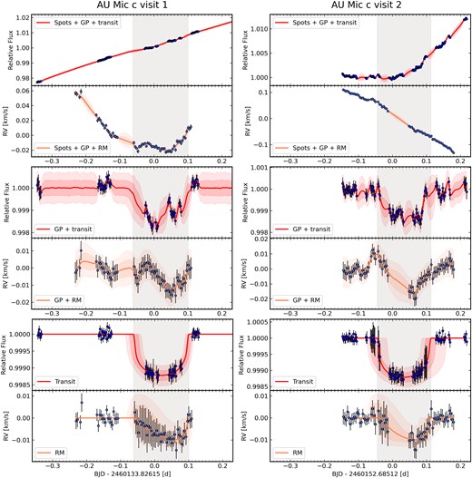
Joint analysis of the first and second transits of AU Mic c. The upper plots show the raw data with lines and contours corresponding to the full model (GP + polynomial + transits). The middle plots show the data and models subtracting the polynomial component. The lower plots show the model and data further subtracting the GP component. For each plot, the model is estimated through 10 000 randomly selected samples with corresponding weights generated from the nested sampling. The solid lines correspond to the weighted median of the samples, while the contours correspond to the 68.3 per cent (which is equivalent to 1|$\sigma$| for a Gaussian distribution) and 95 per cent CIs of the samples. Each of the samples obtained via nested sampling is associated with a weight, which was taken into account when evaluating the percentiles used to compute the CIs. In the middle and lower plots, the data points are the original data minus the weighted median of the samples for the components of the model subtracted, evaluated at the location of the observations, and their error bars are calculated as the quadrature sum of the original error bars and the weighted standard deviation of these samples. The solid lines and the surrounding shaded areas represent the median, 68.3 per cent, and 95 per cent CIs of the transit model. The grey shaded area in each panel indicates the duration of the transit.
The best-fitting model shown in the bottom panel of Fig. 4 and in Fig. 5 displays the one-sided RM signature characteristic of a misaligned orbit (as opposed to a prograde or retrograde one), and the best-fitting (maximum a posteriori) value of the projected spin–orbit angle is |$\lambda \approx 87$| degrees. However, the posterior distribution for |$\lambda$| is bimodal, with a second subsidiary maximum at |$\lambda \approx 34$| degrees, and a width that appears to encompass 0 degree. Formally, we measure |$\lambda =67.8_{-49.0}^{+31.7}$| degrees, where the central value represents the median and the uncertainties encompass the central 68.3 per cent of the posterior distribution. After taking into account their weights from the nested sampling, 89 per cent of the posterior samples correspond to somewhat misaligned orbits (|$\lambda _{\mathrm{c}} \ge 10$| degrees).
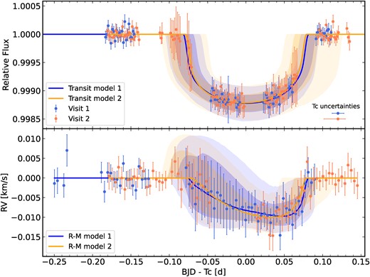
Phase-folded light curve (top) and RV (bottom) observations of the transits of AU Mic b (transit 1 in blue, transit 2 in orange). The polynomial and GP terms used to model the spot signals and residual short-term variations, respectively, have been subtracted from the data, and the vertical error bars incorporate the uncertainty in those model components. The solid line and shaded areas represent the median, 68.3 per cent (|$1\sigma$|), and 95 per cent (|${\approx} 2\sigma$|) CIs of the transit component of the model. The horizontal error bars shown in the top panel represent the |$1\sigma$| uncertainties on mid-transit times |$T_\mathrm{ c}$| of each transit.
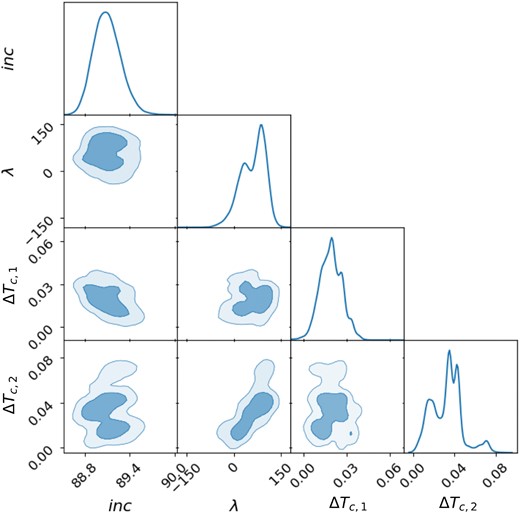
Posterior distribution of key parameters in the joint analysis of the first and second transits of AU Mic c.
The bimodality in the projected spin–orbit angle is partly explained by its strong correlation with the mid-transit times, particularly for the second transit. The latter is itself multimodal, owing to the gaps in the CHEOPS light curve, and this has a knock-on effect on the spin–orbit angle. The derived mid-transit times correspond to TTVs of 27 and 49 min relative to the published ephemerides – somewhat larger than the TTVs previously reported for planet c, though the uncertainties are also large (|${\sim} 15$| min at 1|$\sigma$|).
5 DISCUSSION AND CONCLUSIONS
We have used simultaneous high-precision photometry from CHEOPS and precise RVs from ESPRESSO to measure the projected obliquity of AU Mic relative to the orbital plane of the young, dense sub-Neptune AU Mic c. While inconclusive, our results provide a tentative indication (89 per cent confidence) that the orbit of AU Mic c is misaligned with the spin axis of its host star, and hence also with planet b’s orbit and the debris disc seen at wider separation. Fig. 7 shows a schematic representation of the orbital configuration of planet c relative to the host star and the debris disc, based on the posterior samples from our joint fit of the CHEOPS light curve and ESPRESSO RVs.

Schematic representation of the spin–orbit alignment of planets b and c within the AU Mic system. The stellar disc is colour-coded to represent local RVs, which vary as the star rotates, transitioning from blueshifted on the left to redshifted on the right. The bold green and grey lines represent the inferred orbits for planet b from Palle et al. (2020) and planet c from this work, with arrows indicating the directions of motion for the planets. Thin green and grey lines represent 50 000 randomly selected samples for the orbit of planets b and c, respectively. For the orbit of planet c, the transparency of the thin grey lines scales as the weight of each sample in the nested sampling. The orange arrow marks the axis of stellar rotation. The dark blue arrow marks the orientation of the debris disc.
If this result is confirmed, it will be the first observation of a young (|$\le$|100 Myr) planet on a misaligned orbit. We note that, as the star is seen essentially equator-on, the true obliquity for both planets’ orbits is within a few degrees of the sky-projected value. Only seven other planets with ages |$\le$|100 Myr have measured obliquities to date. In Fig. 8, we show the projected spin–orbit angle versus the age of these planets, together with the measurement of AU Mic c obtained in this work.
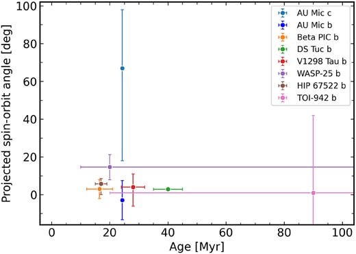
Projected spin–orbit angle of planets in systems younger than 100 Myr. The measurement of AU Mic c obtained in the work is shown in light blue. The measurements of other systems are from Albrecht et al. (2022).
Moreover, very few systems with two transiting planets exhibit large mutual inclinations, irrespective of age. One comparable example is the HD 3167 system, where the close-in super-Earth appears to be on an aligned orbit (Bourrier et al. 2021), while the outer mini-Neptune is on a nearly perpendicular orbit (Dalal et al. 2019).
5.1 Limitations of our measurement
The large uncertainties on our reported value of the projected spin–orbit angle |$\lambda$| for planet c preclude any claim of a significant misalignment at this stage (which would require at least a |$3\sigma$| departure from |$\lambda =0$|).
Degeneracies with other parameters, such as orbital inclination i and especially mid-transit times, are known to affect the measurement of the projected spin–orbit angle, |$\lambda$| (e.g. Narita et al. 2010; Triaud et al. 2010). This highlights the critical role played by CHEOPS in constraining the transit times. On the other hand, even with simultaneous photometry and RVs, we were not able to constrain the transit times as well as we might have hoped given the precision and cadence of our observations, and this had a knock-on effect on the obliquity measurements. This was partly because strong flares coincided with the ingress and egress of both transits, making key parts of the data unusable (in addition to the gaps in each CHEOPS orbit caused by the occultations of the target by the Earth).
5.2 The importance of joint modelling
Before we developed the joint model described in Section 4, our initial attempts at modelling the data involved fitting the CHEOPS light curve first, and then using the posteriors from that fit as priors on the RV fit. When fitting the CHEOPS light curves alone, we were able to model the flares explicitly, rather than masking them out, resulting in somewhat tighter constraints on the mid-transit times. The subsequent fit to the ESPRESSO RVs was restricted to the second transit observation, as the lack of post-transit baseline precluded the use of the first. This fit to the second transit yielded a nominally much more significant detection of a misaligned orbit, with |$\lambda = 108.7\pm 12.5$| degrees. However, the fit of the CHEOPS light curves including flares implied anomalously large TTVs of the order of 50 min – much larger than the 5–10 min TTVs reported for planet c to date (Szabó et al. 2021, 2022; Wittrock et al. 2022, 2023). In addition, there was then a significant tension (around 2|$\sigma$|) between the mid-transit time obtained from the second CHEOPS light-curve fit and from the RV fit (despite the use of the CHEOPS-based prior): the sequential approach does not guarantee a self-consistent fit between the light curve and the RVs. This motivated our decision to model both types of observations simultaneously, rather than sequentially, as reported in Section 4. Doing this required masking the flares, which had the effect of considerably increasing the uncertainty on the mid-transit times, and hence on the projected spin–orbit angle, but allowed us to include the ESPRESSO observations of the first transit into the fit. The result is less precise, but in our view more robust, than the sequential approach. None the less, we note here that the sequential fit supports a significantly misaligned orbit.
Modelling the two observed transits jointly was also important, as the first ESPRESSO observation covered the full transit, but no post-transit baseline, while the gap in the second observation fell during the transit.
5.3 Possible explanations for a misaligned orbit
Despite the tentative nature of our result, it is interesting to speculate as to the mechanisms that could lead to a misaligned orbit for AU Mic c, without disrupting the mutual alignment between the star, disc, and planet b.
One such mechanism is planet–planet scattering. Interactions between planets can lead to significant orbital changes. When these interactions drive relative velocities up to the escape velocity of the most massive body in the system, collisions or giant impacts become likely (Goldreich, Lithwick & Sari 2004; Schlichting 2014). Thus, these collisions typically occur at escape velocity and can result in inclination changes proportional to the ratio of the escape velocity to the local Keplerian velocity. Thus, an order-of-magnitude estimate of the inclination change is |${\sim} v_{\rm col}/v_{\rm Kep}$|. Since |$v_{\rm esc}/v_{\rm Kep}\sim {1/2}$|, then large-inclination changes, similar to the one we have observed, are plausible (e.g. Rasio & Ford 1996; Weidenschilling & Marzari 1996; Lin & Ida 1997; Davies et al. 2014). In the event of a collision, such a scenario would likely result in planet c losing its atmosphere aligning with the abnormal density trend observed between planets b and c derived from mass measurements. However, a collision causing a large inclination is also likely to result in high eccentricity unless it occurred along a specific trajectory that resulted in high inclination and low eccentricity. None the less, the eccentricity of AU Mic c is weakly constrained and may still be relatively significant. Additionally, debris from such a collision could potentially form a disc, allowing the planet to circularize.
Another possibility is a nodal secular resonance, which can drive large misalignments (Ward, Colombo & Franklin 1976; Lai 2014; Owen & Lai 2017). Given the possible presence of an exterior planetary companion (e.g. Donati et al. 2023; Wittrock et al. 2023), this mechanism is a viable explanation for the planet c’s misalignment. In this scenario, the nodal precession frequency of the exterior companion is driven by a dispersing protoplanetary disc, which slowly evolves as the disc disperses. If, during this evolution, the frequency aligns with the nodal precession frequency of planet c, the exterior planet could drive planet c into a highly inclined orbit (Petrovich et al. 2020). In particular, this mechanism drives planets towards polar orbits, broadly consistent with the obliquity we measure. Such secular resonances do not necessarily result in large eccentricities, although they can be induced; however, they do require the system to be configured to allow the precession frequencies to become commensurate during disc dispersal.
A third possibility is Kozai-type interactions with the disc. Kozai-type dynamics cause inclination and eccentricity to oscillate in phases that are 90 degrees out of sync. Since RV monitoring of the system is consistent with a circular orbit for planet c (Zicher et al. 2022; Donati et al. 2023), we might currently be observing AU Mic c in a high-inclination, low-eccentricity phase. Moreover, if the event that caused the tilt in planet c’s orbit happened before the dispersal of the disc, the eccentricity might have been dampened as the planet repeatedly passed through the disc (e.g. Teyssandier, Terquem & Papaloizou 2013; Teyssandier & Terquem 2014).
5.4 Dynamic stability and transit probability
The predicted sky-projected spin–orbit angle of planet c (Table 2) may correspond to a high mutual inclination between the two planets, which raises concerns about the dynamic stability and transit probability of the system.
Petrovich et al. (2020) suggest that large mutual inclinations could lead to eccentric instability, resulting in increased eccentricity, orbit crossings, and overall instability. Conversely, strong planet–planet interactions between planets b and c might stabilize the system, as indicated by Denham et al. (2019), particularly in the presence of general relativity (GR) precession. Due to the significant mutual inclination, planet c would induce a nodal precession on planet b, causing variations in planet b’s impact parameter and leading to transit duration variations (TDVs) as well as the TTVs that have been observed. More accurate predictions of the TTVs and TDVs, requiring detailed N-body calculations, could provide a further test of the mutual inclination of the system.
To check whether the system can be stable, we performed a dynamical analysis in a similar way as for other planetary systems (e.g. Correia et al. 2005, 2010). The system is integrated on a regular 2D grid of initial conditions around the best-fitting solution from table 5 in Wittrock et al. (2023). Each initial condition is integrated for |$5000$| yr, using the symplectic integrator SABAC4 (Laskar & Robutel 2001), with a step size of |$5 \times 10^{-4}$| yr and GR corrections. We then performed a frequency analysis (Laskar 1990, 1993) of the mean longitude of planet c over two consecutive time intervals of 2500 yr, and determined the main frequency, n and |$n^{\prime }$|, respectively. The stability is measured by |$\Delta = \log |1-n^{\prime }/n|$|, the stability index, which estimates the chaotic diffusion of the orbits. A higher absolute value of the stability index indicates that the system is more stable. We note that the stability analysis here does not consider the impact of the debris disc.
In the lower panel of Fig. 9, we present the stability of the system with varying the projected spin–orbit angle8 and the eccentricity of planet c. The colour represents the stability index, with orange and red indicating strongly chaotic unstable trajectories. A stability index below −4 indicates that the system is stable on time-scales around 20 Myr, corresponding to the current age of the AU Mic system. We observe that orbits with eccentricities higher than 0.3 or spin–orbit angles higher than 50 degrees are completely unstable.
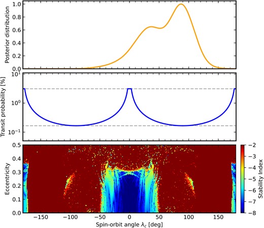
Upper panel: Posterior distribution of the sky-projected spin–orbit angle of AU Mic c |$\lambda _{\mathrm{c}}$|. Middle panel: Transit probability versus |$\lambda _{\mathrm{c}}$|, assuming that AU Mic b is well aligned, estimated following Read, Wyatt & Triaud (2017). Lower panel: Stability analysis of the AU Mic planetary system. For fixed initial conditions (table 5 in Wittrock et al. 2023), the parameter space of the system is explored by varying the projected spin–orbit angle and the eccentricity of planet c. The step size is |$0.9 \ \mathrm{ degree}$| in the spin–orbit angle and 0.0025 in the eccentricity. For each initial condition, the system is integrated over |$5000$| yr and a stability indicator is calculated, which involves a frequency analysis of the mean longitude of planet c. The chaotic diffusion is measured by the variation in the main frequency (see text). Red and orange points correspond to highly unstable orbits.
In comparison, we show the posterior distribution of the measured sky-projected spin–orbit angle of AU Mic c |$\lambda _{\mathrm{c}}$| in the upper panel of Fig. 9. We adopted an eccentricity for planet c of |$0.041_{-0.026}^{+0.047}$| measured from RV modelling in Zicher et al. (2022). The posterior distribution of |$\lambda _{\mathrm{c}}$| reveals a median value around 67 degrees and a maximum a posteriori value around 87 degrees, which lies in an unstable region. However, stability is possible within the uncertainty of |$\lambda _{\mathrm{c}}$| for lower values, especially around the second subsidiary maximum in the posterior distribution around 34 degrees.
To check the transit probability of the two planets, we used the semi-analytical transit probability model presented in Ragozzine & Holman (2010), Brakensiek & Ragozzine (2016) and Read et al. (2017). The input parameters of the model include the radius of the star and the semimajor axis of the two planets, for which we use values reported in Donati et al. (2023) and Wittrock et al. (2023). By assuming that planet b is on a well-aligned orbit, we estimated the double transit probability versus the projected spin–orbit angle of planet c, shown in the middle panel of Fig. 9. Compared to the case where both planets are well aligned, the transit probability is about 1/17 of that scenario when planet c is misaligned with |$\lambda _{\mathrm{c}} = 67.8_{-49.0}^{+31.7}$| degrees.
In summary, a significantly misaligned orbit for planet c is in some degree of tension with dynamical stability arguments, and with the fact that we see both planets in transit. While these arguments alone do not preclude such an orbit, they tend to favour the lower end of the range of mutual inclinations allowed by our analysis and presented in Section 4. Ideally, repeat observations should be carried out to settle the matter.
5.5 Future work
Given the importance of this system and the challenges caused by stellar activity, repeating the observations at a later date would be highly desirable to confirm the result and search for evidence of orbital procession.
The enhanced activity level of AU Mic during our observations compared to observations of the system in 2018–2021 was evidenced by the flares and the strong spot-induced signals seen in both light curves and spectra. We developed a novel method to characterize the flares in the ESPRESSO data, and mitigate their impact on the extracted RVs. This technique could prove valuable for future mass and obliquity measurements of planets around active stars.
The data set presented in this work contains a wealth of information about the spectroscopic signature of the flares, which we intend to investigate further and report on in a future paper.
In principle, it should also be possible to use Doppler tomography techniques to cross-check the results of our RV analysis, as done by Palle et al. (2020) for the ESPRESSO observations of the transit of planet b. However, this would require a modelling framework capable of handling the rotating active regions present on the stellar surface during and around the transits, which is beyond the scope of this work.
ACKNOWLEDGEMENTS
The authors thank Caroline Terquem, Dan Foreman-Mackey, Jiayin Dong, Fei Dai, and Yu Xu for insightful discussions. HY, SA, BK, and OB acknowledge funding from the European Research Council under the European Union’s Horizon 2020 research and innovation programme (grant agreement no. 865624, GPRV). MC acknowledges the SNSF support under grant P500PT_211024. HMC acknowledges funding from a UKRI Future Leader Fellowship, grant number MR/S035214/1. The contributions at the Mullard Space Science Laboratory by EMB have been supported by STFC through the consolidated grant ST/W001136/1. JEO was supported by a Royal Society University Research Fellowship, and JEO’s contribution received funding from the European Research Council (ERC) under the European Union’s Horizon 2020 research and innovation programme (grant agreement no. 853022). This study is based on data collected under the NGTS project at the ESO La Silla Paranal Observatory. The NGTS facility is operated by the consortium institutes with support from the UK Science and Technology Facilities Council (STFC) projects ST/M001962/1 and ST/S002642/1. CHEOPS is an ESA mission in partnership with Switzerland with important contributions to the payload and the ground segment from Austria, Belgium, France, Germany, Hungary, Italy, Portugal, Spain, Sweden, and the United Kingdom. The CHEOPS Consortium would like to gratefully acknowledge the support received by all the agencies, offices, universities, and industries involved. Their flexibility and willingness to explore new approaches were essential to the success of this mission. CHEOPS data analysed in this article will be made available in the CHEOPS mission archive (https://CHEOPS.unige.ch/archive_browser/). ZG was supported by the VEGA grant of the Slovak Academy of Sciences no. 2/0031/22 and by the Slovak Research and Development Agency – the contract no. APVV-20-0148. GyMS acknowledges the support of the Hungarian National Research, Development and Innovation Office (NKFIH) grant K-125015, a PRODEX Experiment Agreement No. 4000137122, the Lendület LP2018-7/2021 grant of the Hungarian Academy of Science, and the support of the city of Szombathely. DG gratefully acknowledges financial support from the CRT Foundation under grant no. 2018.2323 (‘Gaseous or rocky? Unveiling the nature of small worlds’). ACMC acknowledges support from the FCT, Portugal, through the CFisUC projects UIDB/04564/2020 and UIDP/04564/2020, with DOI identifiers 10.54499/UIDB/04564/2020 and 10.54499/UIDP/04564/2020, respectively. ACMC, AD, BE, KG, and JK acknowledge their role as ESA-appointed CHEOPS Science Team Members. AB was supported by the SNSA. MNG is the ESA CHEOPS Project Scientist and Mission Representative, and as such also responsible for the Guest Observers (GO) Programme. MNG does not relay proprietary information between the GO and GTO programmes, and does not decide on the definition and target selection of the GTO Programme. TGW acknowledges support from the UKSA and the University of Warwick. YA acknowledges support from the Swiss National Science Foundation (SNSF) under grant 200020_192038. DB, EP, and IR acknowledge financial support from the Agencia Estatal de Investigación of the Ministerio de Ciencia e Innovación MCIN/AEI and the ERDF ‘A way of making Europe’ through projects PID2019-107061GB-C61, PID2019-107061GB-C66, PID2021-125627OB-C31, PID2021-125627OB-C32, and PID2023-150468NB-I00, from the Centre of Excellence ‘Severo Ochoa’ award to the Instituto de Astrofísica de Canarias (CEX2019-000920-S), from the Centre of Excellence ‘María de Maeztu’ award to the Institut de Ciències de l’Espai (CEX2020-001058-M), and from the Generalitat de Catalunya/CERCA programme.SCCB acknowledges support from FCT through FCT contract no. IF/01312/2014/CP1215/CT0004. LB, VN, IP, GPi, RR, and GS acknowledge support from CHEOPS ASI-INAF agreement no. 2019-29-HH.0. CB and AES acknowledge support from the Swiss Space Office through the ESA PRODEX program. ACC acknowledges support from STFC consolidated grant number ST/V000861/1, and UKSA grant number ST/X002217/1. PEC was funded by the Austrian Science Fund (FWF) Erwin Schroedinger Fellowship, program J4595-N. This project was supported by the CNES. This work was supported by FCT – Fundação para a Ciência e a Tecnologia – through national funds and by FEDER through COMPETE2020 through the research grants UIDB/04434/2020, UIDP/04434/2020, and 2022.06962.PTDC. ODSD was supported in the form of work contract (DL 57/2016/CP1364/CT0004) funded by national funds through FCT. B-OD acknowledges support from the Swiss State Secretariat for Education, Research and Innovation (SERI) under contract number MB22.00046. This project has received funding from the Swiss National Science Foundation for project 200021_200726. It has also been carried out within the framework of the National Centre of Competence in Research PlanetS supported by the Swiss National Science Foundation under grant 51NF40_205606. The authors acknowledge the financial support of the SNSF. MF and CMP gratefully acknowledge the support of the Swedish National Space Agency (DNR 65/19 and 174/18). MG is an F.R.S.-FNRS Senior Research Associate. CH acknowledges the European Union H2020-MSCA-ITN-2019 under grant agreement no. 860470 (CHAMELEON), and the HPC facilities at the Vienna Science Cluster (VSC). KWFL was supported by Deutsche Forschungsgemeinschaft grants RA714/14-1 within the DFG Schwerpunkt SPP 1992, Exploring the Diversity of Extrasolar Planets. This work was granted access to the HPC resources of MesoPSL financed by the Region Ile de France and the project Equip@Meso (reference ANR-10-EQPX-29-01) of the programme Investissements d’Avenir supervised by the Agence Nationale pour la Recherche. ML acknowledges support of the Swiss National Science Foundation under grant number PCEFP2_194576. PFLM acknowledges support from STFC research grant number ST/R000638/1. This work was also partially supported by a grant from the Simons Foundation (PI: Queloz, grant number 327127). NCS acknowledges funding by the European Union (ERC, FIERCE, 101052347). Views and opinions expressed are, however, those of the author(s) only and do not necessarily reflect those of the European Union or the European Research Council. Neither the European Union nor the granting authority can be held responsible for them. SGS acknowledges support from FCT through FCT contract nos CEECIND/00826/2018 and POPH/FSE (EC). The Portuguese team thanks the Portuguese Space Agency for the provision of financial support in the framework of the PRODEX Programme of the European Space Agency (ESA) under contract number 4000142255. VVG is an F.R.S.-FNRS Research Associate. JV acknowledges support from the Swiss National Science Foundation (SNSF) under grant PZ00P2_208945. EV acknowledges support from the ‘DISCOBOLO’ project funded by the Spanish Ministerio de Ciencia, Innovación y Universidades under grant PID2021-127289NB-I00. NAW acknowledges UKSA grant ST/R004838/1. ML acknowledges the support from the UKRI grant (grant number: EP/X027562/1).
This study is based on observations made with the ESO’s VLT at Paranal Observatory under programme 111.24VF. This study uses CHEOPS data observed as part of the GTO programme CH_PR00071.
DATA AVAILABILITY
The photometric and RV data used in this work are publicly available at CDS via anonymous ftp.
Footnotes
A visit is a sequence of successive CHEOPS orbits about the Earth that are devoted to observing a single target. CHEOPS revolves around the Earth every |$\sim$|99 min in a Sun-synchronous, low-Earth orbit (700-km altitude).
Tested using version 14.1.3 of the DRP (Hoyer et al. 2020).
These interruptions happen once per CHEOPS orbit when the target is occulted by the Earth, or it is barely visible due to stray light from the illuminated Earth limb or particle hits during passages above the South Atlantic anomaly.
The flux-weighted mean wavelength of the customized CCF mask used for the ESPRESSO data is 624.4 nm. This closely aligns with the centre of mass of the CHEOPS passband, which ranges from 400 to 1100 nm. Therefore, we applied the same limb-darkening coefficients to both the CHEOPS and ESPRESSO data.
We assume |$i_* \approx i_{\mathrm{b}} \approx i_{\mathrm{c}} \approx 90 \ \mathrm{ degrees}$| (Wittrock et al. 2023), and thus |$\lambda _{\mathrm{c}} \approx \Omega$| (Fabrycky & Winn 2009), where |$\lambda _{\mathrm{c}}$| is the spin–orbit angle and |$\Omega$| is the longitude of the node of planet c.
REFERENCES
APPENDIX A: TABLE FOR DERIVED VALUES OF ALL FREE PARAMETERS AND THEIR POSTERIOR DISTRIBUTIONS
The parameters of the joint fit described in Section 4 are listed in Table A1, which gives the priors adopted over each parameter and the values inferred from the fit. LC-sig, LC-rho, LC-jit, RV-sig, RV-rho, and RV-jit are GP hyperparameters in the model. sig is the overall variance, rho is the time-scale in the Matérn 5/2 kernel representing how quickly the correlation between points decreases with distance, and jit is the jitter term. The 1D and 2D posterior distributions are shown in Fig. A1.
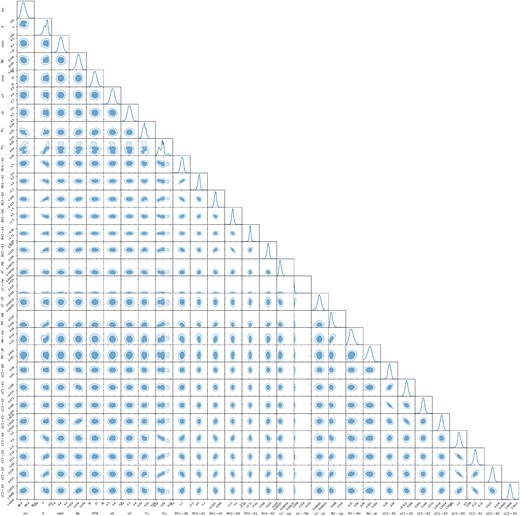
Posterior distribution of all free parameters in the joint analysis (CHEOPS photometry and ESPRESSO RVs) of the first and second transits of AU Mic c.
Priors and inferred values for all free parameters from the joint analysis (CHEOPS photometry and ESPRESSO RVs) of the first and second transits of AU Mic c.
| Parameter | Prior | Value|$^{a}$| | 95 per cent CI |
|---|---|---|---|
| i | |$\mathcal {N}[89.22,0.21]$| | |$89.09_{-0.17}^{+0.18}$| | 88.77–89.47 |
| |$\lambda$| | |$\mathcal {U}[-180.0,180.0]$| | |$67.8_{-49.0}^{+31.7}$| | −|$23.2$|–120.7 |
| |$v \sin i$| | |$\mathcal {N}[8.5,0.2]$| | |$8.49_{-0.19}^{+0.19}$| | 8.10–8.88 |
| |$R_\mathrm{p}/R_\mathrm{s}$| | |$\mathcal {N}[0.0311,0.0028]$| | |$0.0320_{-0.0019}^{+0.0019}$| | 0.0281–0.0356 |
| |$a/R_\mathrm{s}$| | |$\mathcal {N}[32.05,1.0]$| | |$32.35_{-0.95}^{+0.96}$| | 30.49–34.24 |
| |$u_1$| | |$\mathcal {N}[0.47,0.1]$| | |$0.51_{-0.09}^{+0.09}$| | 0.33–0.70 |
| |$u_2$| | |$\mathcal {N}[0.30,0.1]$| | |$0.32_{-0.09}^{+0.09}$| | 0.13–0.51 |
| |$T_{\mathrm{ c},1}-2460\,133.826\,15^{b}$| (d) | |$\mathcal {U}[-0.02,0.10]$| | |$0.0191_{-0.0076}^{+0.0078}$| | 0.0046–0.0343 |
| |$T_{\mathrm{ c},2}-2460\,152.685\,12^{b}$| (d) | |$\mathcal {U}[-0.02,0.10]$| | |$0.0341_{-0.0183}^{+0.0095}$| | 0.0073–0.0703 |
| RV1-b0 | |$\mathcal {U}[-3.0,3.0]$| | |$1.5982_{-0.2583}^{+0.2411}$| | 1.0643–2.0453 |
| RV1-b1 | |$\mathcal {U}[-1.0,1.0]$| | |$0.0540_{-0.0366}^{+0.0312}$| | −|$0.0225$|–0.1170 |
| RV1-b2 | |$\mathcal {U}[-3.0,3.0]$| | |$-0.0130_{-0.0044}^{+0.0040}$| | −|$0.0218$|–−|$0.0047$| |
| RV2-b0 | |$\mathcal {U}[-3.0,3.0]$| | |$-0.7591_{-0.2538}^{+0.2436}$| | −|$1.2881$|–−|$0.2426$| |
| RV2-b1 | |$\mathcal {U}[-1.0,1.0]$| | |$-0.7207_{-0.0205}^{+0.0204}$| | −|$0.7683$|–−|$0.6750$| |
| RV2-b2 | |$\mathcal {U}[-3.0,3.0]$| | |$0.0228_{-0.0043}^{+0.0042}$| | 0.0136–0.0315 |
| LC-sig | |$\mathcal {U}[0.0,0.01]$| | |$0.000\,33_{-0.000\,04}^{+0.000\,04}$| | 0.000 26–0.000 44 |
| LC-rho | |$\mathcal {U}[0.006,0.042]$| | |$0.0064_{-0.0003}^{+0.0008}$| | 0.0060–0.0087 |
| LC-jit | |$\mathcal {U}[0.0,0.001]$| | |$0.0001_{-0.0000}^{+0.0000}$| | 0.0000–0.0001 |
| RV-sig | |$\mathcal {U}[0.0,0.1]$| | |$0.0050_{-0.0013}^{+0.0018}$| | 0.0028–0.0092 |
| RV-rho | |$\mathcal {N}[0.018, 0.01]$| | |$0.0234_{-0.0063}^{+0.0071}$| | 0.0119–0.0383 |
| RV-jit | |$\mathcal {U}[0.0,0.01]$| | |$0.0011_{-0.0004}^{+0.0004}$| | 0.0002–0.0018 |
| LC1-b0 | |$\mathcal {U}[-2.0,2.0]$| | |$0.0456_{-0.0168}^{+0.0167}$| | 0.0125–0.0795 |
| LC1-b1 | |$\mathcal {U}[-2.0,2.0]$| | |$-0.0078_{-0.0033}^{+0.0034}$| | −|$0.0145$|–−|$0.0011$| |
| LC1-b2 | |$\mathcal {U}[-2.0,2.0]$| | |$0.0649_{-0.0013}^{+0.0013}$| | 0.0623–0.0675 |
| LC1-b3 | |$\mathcal {U}[-2.0,2.0]$| | |$1.0022_{-0.0002}^{+0.0001}$| | 1.0019–1.0025 |
| LC2-b0 | |$\mathcal {U}[-2.0,2.0]$| | |$0.0408_{-0.1055}^{+0.1210}$| | −|$0.1928$|–0.2729 |
| LC2-b1 | |$\mathcal {U}[-2.0,2.0]$| | |$0.1271_{-0.0149}^{+0.0141}$| | 0.0972–0.1560 |
| LC2-b2 | |$\mathcal {U}[-2.0,2.0]$| | |$0.0213_{-0.0029}^{+0.0024}$| | 0.0158–0.0271 |
| LC2-b3 | |$\mathcal {U}[-2.0,2.0]$| | |$1.0010_{-0.0002}^{+0.0002}$| | 1.0007–1.0014 |
|$^{a}$|Median and 68.3 per cent CI.
|$^{b}$|Transit times are quoted relative to the published ephemerides of Wittrock et al. (2023), namely |$T_\mathrm{ c}=2458\,342.2240$| and |$P_{\mathrm{c}}=18.858\,970$| d.
APPENDIX B: NGTS LIGHT-CURVE ANALYSIS
We performed a stand-alone analysis of the NGTS data collected on the nights of 2023 July 7 and 26. Initially, we attempted an agnostic analysis where the transit mid-point times and the planet-to-star radius ratio were allowed to vary freely. However, the NGTS data are significantly impacted by the presence of clouds during both observations. The light curves also display significant short-term variability, which may be due to flares or spots, and ramps at the beginning and the end of the observations, which are most likely due to insufficient comparison stars of a brightness and colour similar to AU Mic. Due to this, the results of this agnostic analysis are highly sensitive to the out-of-transit flux baseline model used and the priors chosen. Therefore, in this instance we feel that these NGTS observations are unable to provide independent constraints on the planet parameters or transit timing. However, the photometric precision of the NGTS measurements is high enough that, dependent on the exact transit timing, the data may provide evidence against the transit timing reported by the CHEOPS–ESPRESSO observations. We therefore perform a transit analysis to check for any inconsistency between the NGTS observations and the results of the CHEOPS–ESPRESSO joint analysis.
For this analysis, we compute the transit models using the batmanpython package (Kreidberg 2015). The only planet parameter we allow to vary is the transit mid-point time, |$T_{\rm C}$|. For this parameter, we use a truncated Gaussian prior with a mean and standard deviation taken from the median and 68.3 per cent CI from the CHEOPS–ESPRESSO joint analysis and a strict upper limit set by the 95 per cent CI from the joint analysis. The values of these are provided in Table A1. We fix the remaining planet parameters – orbital period, P, planet-to-star radius ratio, |$R_{\rm P}/R_{\ast }$|, semimajor axis scaled to the stellar radius, |$a/R_{\ast }$|, orbital inclination, i, eccentricity, e, argument of periastron, |$\omega$|, and the quadratic limb-darkening coefficients – to the median values from the joint analysis (Table A1). Simultaneously to varying the transit mid-point time we fit the out-of-transit flux baseline using a quadratic polynomial trend in time.
We explored the joint posterior over the fit parameters using Markov chain Monte Carlo using the emcee (Foreman-Mackey et al. 2013) package. 12 walkers were run for a burn-in phase of 3000 steps followed by a further 15 000 steps ‘production’ run. The resulting parameters from this analysis are provided in Table B1 and the best-fitting models are shown in Fig. B1. The resulting transit mid-point times from this analysis are |$2460133.8485^{+0.0061}_{-0.0090}$| BJD-TDB and |$2460152.7360^{+0.0013}_{-0.0014}$| BJD-TDB for visits one and two, respectively. For the night of 2023 July 7, the NGTS data are fully consistent with the results of the CHEOPS–ESPRESSO joint analysis. For the night of 2023 July 26, the NGTS observations suggest a slightly later transit than the 68.3 per cent CI of the CHEOPS–ESPRESSO joint analysis but fully support the presence of the transit occurring during the 95 per cent CI.
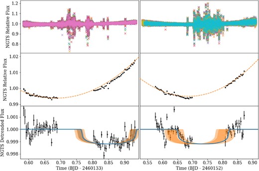
NGTS photometric observations of the AU Mic c transits. The left and right columns show the first and second visits, respectively. The top row shows the full observations for all telescopes used, with data from each individual telescope plotted using a different colour. The middle row shows the data with the cloud-affected portion removed, and with the data from all telescopes binned together at a time-scale of 5 min (the binning is performed for visualization purposes only; the analysis was performed on the unbinned data). The orange dashed line in the middle row shows the best-fitting polynomial component to the NGTS data. The bottom row shows the data after subtracting the polynomial component. The blue line shows the best-fitting model from the NGTS analysis with the blue shaded region showing the 68 per cent CI. The dark and light orange shaded regions give the 67.3 and 95 per cent CIs, respectively, from the CHEOPS–ESPRESSO joint analysis.
Results obtained from the analysis of the NGTS observations. The parameter values are the median posterior values and the uncertainties give the 16 and 84 percentile ranges of the posteriors.
| Name | Symbol | Value | |
|---|---|---|---|
| 2023 July 7 | 2023 July 26 | ||
| Transit mid-point time | |$T_{\rm C}$| | |$2460\,133.8485^{+0.0061}_{-0.0090}$| | |$2460\,152.7360^{+0.0013}_{-0.0014}$| |
| Constant detrending coefficient | |$c_{\rm 0}$| | |$1.1738^{+0.0043}_{-0.0044}$| | |$1.1968\pm 0.0031$| |
| Quadratic detrending coefficient | |$c_{\rm 1}$| | |$-0.524\pm 0.012$| | |$-0.5876^{+0.0086}_{-0.0087}$| |
| Quadratic detrending coefficient | |$c_{\rm 2}$| | |$0.3819^{+0.0079}_{-0.0080}$| | |$0.4278^{+0.0060}_{-0.0058}$| |
