


ABSTRACT
We present a comprehensive examination of the three latest versions of the L-galaxies semi-analytic galaxy formation model, focusing on the evolution of galaxy properties across a broad stellar mass range (|$10^7\:{\rm M}_{\odot }\lesssim {M_\star }\lesssim 10^{12}\:{\rm M}_{\odot }$|) from |$z=0$| to |$z\simeq 10$|. This study is the first to compare predictions of L-galaxies with high-redshift observations well outside the original calibration regime, utilizing multiband data from surveys such as SDSS, CANDELS, COSMOS, HST, JWST, and ALMA. We assess the models’ ability to reproduce various time-dependent galaxy scaling relations for star-forming and quenched galaxies. Key focus areas include global galaxy properties such as stellar mass functions, cosmic star formation rate density, and the evolution of the main sequence of star-forming galaxies. Additionally, we examine resolved morphological properties such as the galaxy mass–size relation, alongside core |$(R\lt 1\, {\rm {kpc}})$| and effective |$(R\lt R_{\rm {e}})$| stellar-mass surface densities as a function of stellar mass. This analysis reveals that the L-galaxies models are in qualitatively good agreement with observed global scaling relations up to |$z\simeq 10$|. However, significant discrepancies exist at both low and high redshifts in accurately reproducing the number density, size, and surface density evolution of quenched galaxies. These issues are most pronounced for massive central galaxies, where the simulations underpredict the abundance of quenched systems at |$z\ge 1.5$|, reaching a discrepancy of a factor of 60 by |$z\approx 3$|, with sizes several times larger than observed. Therefore, we propose that the physical prescriptions governing galaxy quenching, such as AGN feedback and processes related to merging, require improvement to be more consistent with observational data.
1 INTRODUCTION
In recent years, significant advancements in telescope and detector technologies, coupled with improved computational capabilities, have led to significant progress in our understanding of galaxy formation and evolution. Observations of galaxies in large surveys in the early 2000s allowed us to characterize global galaxy properties such as stellar mass (e.g. Cole et al. 2001; Bell et al. 2003; Kauffmann et al. 2003; Drory et al. 2009; Marchesini et al. 2009; Peng et al. 2010b; Whitaker et al. 2011; Fontana et al. 2014) and star formation rates (e.g. Lilly et al. 1996; Madau et al. 1996; Kennicutt 1998; Madau, Pozzetti & Dickinson 1998; Bell & de Jong 2001; Brinchmann et al. 2004; Daddi et al. 2007; Elbaz et al. 2007; Evans Neal J. et al. 2009; Santini et al. 2009; Speagle et al. 2014) for samples of hundreds of thousands of galaxies at low redshifts and to study global galaxy scaling relations. More recent observations have allowed us not only to characterize the same global galaxy properties at high redshifts (e.g. Ilbert et al. 2013; Muzzin et al. 2013; Schreiber et al. 2015; Stefanon et al. 2021; Harikane et al. 2022, 2023, 2024; Santini et al. 2022; Weaver et al. 2023) but also resolved properties such as morphology and size, stellar surface mass density and star formation rate profiles as well as deviations from axisymmetry in these systems (e.g. Wuyts et al. 2013; van der Wel et al. 2014b; Förster Schreiber & Wuyts 2020; Tacconi, Genzel & Sternberg 2020; Conselice et al. 2024; Huertas-Company et al. 2024). Recent studies have further delved into local Galactic properties, investigating different evolutionary processes such as stellar content, radial migration, star formation, and chemical enrichment histories (e.g. Snaith et al. 2015; Sysoliatina & Just 2021; Gaia Collaboration 2023; Golovin et al. 2023; Katz et al. 2023), thereby providing a comprehensive view of galaxy evolution on all scales and epochs.
Galaxies have structure over a very wide range of physical scales, and the physical processes that determine these structures can be quite different on small and large scales. The field has seen the development of a variety of simulation techniques (see Somerville & Davé 2015, for a review) such as semi-analytical models (e.g. Kauffmann, White & Guiderdoni 1993; Somerville & Primack 1999; De Lucia & Blaizot 2007; Just & Jahreiß 2010; Guo et al. 2011; Croton et al. 2016; Cora et al. 2018; Lagos et al. 2018; Henriques et al. 2020), cosmological hydrodynamical models (e.g. Dubois et al. 2014; Hopkins et al. 2014; Vogelsberger et al. 2014; Schaye et al. 2015; McCarthy et al. 2017; Hopkins et al. 2018; Pillepich et al. 2018; Vogelsberger et al. 2020; Villaescusa-Navarro et al. 2021; Schaye et al. 2023; Bhagwat et al. 2024), and zoom-in simulations of galaxies that aim to resolve the detailed internal structure of galaxies (e.g. Naab et al. 2014; Wang et al. 2015; Grand et al. 2017; Tremmel et al. 2019; Dubois et al. 2021; Wetzel et al. 2023; Grand et al. 2024).
The progress of these simulations has enabled the creation of highly accurate representations of the observable universe within the |$\Lambda {}\text{CDM}$| cosmological framework (Planck Collaboration VI 2020). Such recent successes are a testament to the realistic nature of these simulations as they now start to be able to reproduce not only global galaxy properties but also how the material is distributed within galaxies (e.g. Pillepich et al. 2019; Henriques et al. 2020).
To interpret new observations from the most modern galaxy surveys and telescopes, such as the Dark Energy Spectroscopic Instrument (DESI; DESI Collaboration 2016), the Sloan Digital Sky Survey-V (SDSS-V; Kollmeier et al. 2017), the 4-metre Multi-Object Spectroscopic Telescope (4MOST; de Jong et al. 2019), the JWST Advanced Deep Extragalactic Survey (JADES; Eisenstein et al. 2023), and the Cosmic Evolution Early Release Science Survey (CEERS; Finkelstein et al. 2023), theoretical models based either on hydrodynamical or semi-analytical models must refine their capabilities. This is crucial for maintaining consistency with the local and global galaxy properties of observations throughout the evolution of time.
While offering high accuracy and realism, cosmological hydrodynamical simulations demand substantial computational resources, making it difficult to explore large volumes at high resolution or navigate effectively the multidimensional parameter space of uncertainties in the physical treatment of processes such as star formation, supernova (SN), and active galactic nuclei (AGNs) feedback (Nelson et al. 2019; Pillepich et al. 2019; Bhagwat et al. 2024). These challenges are addressed by semi-analytical models, which significantly accelerate the model’s execution time by effectively modelling key galaxy evolution physical processes (Kauffmann et al. 1993; Somerville & Primack 1999) in parametrized form instead of solving the equations of hydrodynamics for very large systems of resolution elements.
A semi-analytical approach to galaxy evolution incorporates fundamental baryonic processes that govern galaxy formation and evolution such as the infall of the gas into the dark matter haloes, gas cooling, star formation and stellar feedback, chemical evolution, supermassive black hole (SMBH) formation and growth, AGN feedback, and so on. This method builds upon the foundation of dark matter halo merger trees, which are either constructed through Monte Carlo realizations or derived from particle data of dark matter-only simulations (e.g. Kauffmann et al. 1993, 1999; Somerville & Primack 1999; Springel et al. 2001; De Lucia et al. 2006). Lacking a direct implementation of hydrodynamical processes, semi-analytical models realize a parametrized modelling of gas-physical processes on top of dark matter halo merger trees, necessitating analytical approximations. Consequently, the development of such models relies on various simplifying assumptions that can introduce modelling uncertainties in the outcomes. For example, earlier semi-analytical models have assumed that the entire hot gas reservoir of a galaxy is stripped upon crossing the virial radius of the halo (e.g. Kauffmann et al. 1999; Croton et al. 2006). In contrast, modern semi-analytical models, like the L-galaxies model, also known as the Munich model (Ayromlou et al. 2021b), propose a gradual and time-dependent gas stripping mechanism, enabling satellite galaxies to retain a portion of their gas for extended periods.
Galaxies are generally classified into two groups: star-forming galaxies (SFGs) and passive or quiescent galaxies (QGs), based on their star formation activity. Various quenching mechanisms that can turn a galaxy into a passive system have been identified, including intrinsic quenching due to stellar and AGN feedback (Kauffmann et al. 2003; Di Matteo, Springel & Hernquist 2005; Elbaz et al. 2007; Beckmann et al. 2017), and environmental quenching (Gunn & Gott 1972; Springel, Di Matteo & Hernquist 2005b; Peng et al. 2010b; Peng, Maiolino & Cochrane 2015). The diverse array of galaxies, varying in size, morphology, and other characteristics, plays an essential role in our empirical understanding of galaxy evolution (e.g. Conselice 2014; Naab & Ostriker 2017). Notably, the study of galaxy scaling relations, reflecting the complex interplay between attributes like mass, size, luminosity, colour, star formation rate, and several other galaxy properties, has long been a fundamental cornerstone in comprehending the complex interplay between various galaxy attributes as a function of cosmic time (see Stark 2016; Förster Schreiber & Wuyts 2020; D’Onofrio, Marziani & Chiosi 2021, for a review). Such correlations along with their slope, zero point, and scatter (e.g. Stone, Courteau & Arora 2021; Popesso et al. 2023) can help us uncover the complex physics behind the formation and evolution of SFGs and QGs. Moreover, galaxy scaling relations can be used to inform and enrich new generations of galaxy formation models.
This work provides a comprehensive and contemporary examination of the three recent versions or flavours of the L-galaxies semi-analytic model. These correspond to the most recent and independently calibrated versions of the L-galaxies framework, namely: Henriques et al. (2015, 2020) and Ayromlou et al. (2021b), all of which were designed as enhancements over their corresponding predecessors.
Our objective is to conduct an extensive comparison of the results generated by these models across a wide range of masses and redshifts, to see how well they agree with recent observational scaling relations, particularly at high redshift (|$z\gtrsim 2$|). Our focus includes exploring the stellar mass functions, the cosmic star formation density, the main sequence of SFGs (i.e. the |${\rm SFR}-M_{\star }$|) relation, the galaxy mass–size relation and the evolution of the core (|$R\lt 1\:{\rm kpc}$|) and effective (|$R\lt R_{\rm e}$|) stellar mass surface density. These relations are analysed for both SFGs and QGs independently. While some of these relations have been thoroughly studied at low redshift (Croton et al. 2016; Lagos et al. 2018; Ayromlou et al. 2021b), a comprehensive exploration across a wide mass and redshift range is yet to be realized for a semi-analytical model implementation. Furthermore, we supplement our analysis with an examination of baryonic processes that influence galaxy quenching, using the latest version of the L-galaxies model (Ayromlou et al. 2021b). This includes an analysis of the distribution of baryons and gas content within haloes, as well as the relative distribution of black holes, hot gas, and cold gas in quenched and star-forming galaxies. This comprehensive comparative analysis serves a dual purpose: not only does it emphasize important benchmarks of our current understanding of the L-galaxies model, but it also pinpoints the specific areas where model enhancements are needed. By extending our investigation to encompass a broader range of mass and redshift, this work identifies key areas for improvement. The refinement and further development of the L-galaxies semi-analytical model are planned for future projects, which will be informed by the findings of this study. These efforts will focus on addressing the discrepancies identified here and improving the implementation of physical processes in the model to achieve better consistency with observational data.
In this paper, we assume a |$\Lambda {}\text{CDM}$| cosmology with |$\Omega _{\Lambda }=0.69$|, |$\Omega _{\rm b}=0.049$|, |$\Omega _{\rm m}=0.315$|, and |$\mathrm{H_{0}=67.3\,\,km\,\,s^{-1}\,\,Mpc^{-1}}$| (Planck Collaboration XIII 2016). All magnitudes are in the AB photometric system (Oke & Gunn 1983), and a Chabrier (2003) initial mass function (IMF) is used throughout this analysis unless stated otherwise.
This paper is organized as follows. Section 2 summarizes the different observational low and high redshift galaxy scaling relations used in this work. In Section 3, we outline the framework of the L-galaxies semi-analytical and briefly describe the key baryonic processes relevant to this study. Section 4 presents the comparison of the model results with the observational galaxy scaling relations for star-forming and quenched systems. Section 5 focuses on baryonic physics which controls galaxy quenching and Section 6 offers a discussion of these findings and similar works. Lastly, Section 7 summarizes our study’s results and presents our conclusions.
2 SUMMARY OF OBSERVATIONAL DATA COMPILATIONS
In this section, we provide a concise overview of the low to high redshift observational metrics and galaxy scaling relations explored in this paper. These correlations serve as key benchmarks, offering insights into the physical processes within galaxies and guiding the refinement of galaxy evolution models.
2.1 Stellar mass functions
The galaxy stellar mass function (SMF) is defined as the number of galaxies per unit volume in stellar mass bins at a given redshift. Understanding its evolution helps us understand various effects of physical processes that govern galaxy evolution (e.g. Li & White 2009; Peng et al. 2010b). Much progress has been made recently in our understanding of this relation thanks to deep surveys probing the stellar mass function down to lower masses and higher redshifts (e.g. Ilbert et al. 2013; Muzzin et al. 2013; Tomczak et al. 2014; McLeod et al. 2021; Santini et al. 2022; Weaver et al. 2023).
Galaxies can generally be classified as SFGs which boast active star formation, or QGs which have little to no star formation activity. The quenching mechanism of a galaxy can be due to the heating or removal of gas by an AGN or SN feedback. This is sometimes called ‘mass quenching’ because of the strong mass-dependent effects of these two processes. Removal of gas by SN-driven winds is more efficient in low-mass galaxies, whereas the most massive black holes (BH) that give rise to the most powerful AGN are located in the most massive galaxies. Alternatively, quenching can be due to environmental effects such as mergers, tidal interactions, and ram-pressure stripping (see Peng et al. 2010b; Wetzel et al. 2013; Man & Belli 2018).
To gain deeper insights into how diverse processes impact the structure and evolution of the SMF, we analyse the star-forming galaxy stellar mass function (SFG SMF), the quiescent galaxy stellar mass function (QG SMF), and the combined representation of the two, the total SMF.
Studies have found that the galaxy stellar mass function is well described by the empirical Schechter function (Schechter 1976) with an exponential downturn at a characteristic mass and a power law at low masses with a slope that has little redshift evolution (Ilbert et al. 2013; Tomczak et al. 2014; Weaver et al. 2023). However, the influence of physical processes on the shape of the SMF is still unclear. Peng et al. (2010b) suggest that a single Schechter shape is due to environmental effects on galaxies in the local universe, while a double Schechter curve can arise due to a combination of both, environmental and mass quenching processes. At |$z\gtrsim 7$|, deviations from the Schechter function have been observed, with the SMF being better described by a power law (e.g. Stefanon et al. 2021). Understanding the evolution of the observed SMF is critical, as it represents one of the most reliable observables used in galaxy formation simulations. The L-galaxies models, for example, employ the SMF at |$z=0$|, 1, and 2 for calibration purposes.
In this work, we utilize the observed SMF from Weaver et al. (2023), where the authors employ the COSMOS2020 photo-z catalogue (Weaver et al. 2022) to present an extensive study on the assembly and quenching of star formation in galaxies. This work provides parametrizations of the shape and evolution of the total SMF up to |$z\sim 7.5$|, and SFG and QG SMF up to |$z\sim 5.5$|. Galaxies are divided into these two classes using the NUVrJ colour–colour selection criterion (Ilbert et al. 2013). The study also highlights challenges in measuring rest-frame J-band fluxes beyond |$z\sim 3$| in Spitzer/IRAC bands, making these measurements reliant on the modelling. By |$z\sim 5$|, the rest-frame r-band requires extrapolation, making it statistically difficult to separate QGs and dusty SFGs. Therefore, it is crucial to acknowledge that the selection of QGs between |$3 \lt z \lesssim 5.5$| is fraught with a higher degree of uncertainty.
The Weaver et al. (2023) study reports a smooth, monotonic evolution in the galaxy SMF at all masses since |$z \sim 7.5$| with consistent growth in the number of star-forming systems (since |$z\sim 5.5$|) and a shift towards a larger number of QG systems at lower redshifts. The SMF of the quenched systems also illustrates a buildup of low mass galaxies up to |$z\sim 1.5$|, along with a higher abundance of massive quenched systems at lower redshifts compared to previous reports (Ilbert et al. 2013; Davidzon et al. 2018). While the SFGs display a double Schechter form at lower redshifts, flattening into a power-law-like form at higher redshifts, the QGs show a more rapid decline in their normalization and a steepening low-mass end slope over time.
It is important to note that the derived value of the low mass end of the SMFs, especially for the quenched systems, can be in error because of mass incompleteness. Additionally, the Weaver et al. (2023) study also addresses the presence and evolution of low-mass quiescent systems at redshifts |$z \gt 1.5$|. Although COSMOS2020 data suggests that the low mass QGs appear to effectively vanish at |$z \gt 1.5$|, evidence from Santini et al. (2022) points to the existence of |$M_\star \lt 10^9 \, {\rm M}_{\odot }$| quiescent systems beyond this redshift. Their study is from a significantly smaller effective area compared to the COSMOS2020 study. We note that the total SMF by Weaver et al. (2023) is consistent with previous work done by Ilbert et al. (2013), Tomczak et al. (2014), Grazian et al. (2015), and Stefanon et al. (2021). It has also been compared with predictions from a number of cosmological galaxy formation simulations, for example, EAGLE (Furlong et al. 2015), SHARK (Lagos et al. 2018), and Illustris TNG (Pillepich et al. 2018).
2.2 Cosmic star formation rate density
The cosmic SFR density (CSFRD) quantifies the mass of stars formed per unit volume and unit time at a given redshift. It serves as a fundamental metric for understanding the underlying processes regulating star formation and galactic evolution. This metric’s significance lies in its direct linkage to the stellar mass and the gas reservoirs within galaxies. In this work, we compare our findings to those from Madau & Dickinson (2014), which used data from various publications spanning 2006–2013, derived from different instruments from |$z\sim 0$| up to |${z\sim 8}$|. Additionally, we incorporate insights from Harikane et al. (2022), who employ data from the Subaru/Hyper Suprime-Cam survey (Aihara et al. 2018) and the Canada-France-Hawaii (CFHT) Large Area U-band Survey (Sawicki et al. 2019), focusing on |$z=2-7$|.
From both studies, a consistent picture emerges where the star formation rate (SFR) density peaks approximately at redshift |$z\sim 1.9$| before entering an exponential decline. It should be noted that the exact slope of the high redshift decline is still debated (see Bouwens et al. 2012; Rowan-Robinson et al. 2016; Driver et al. 2018; Bouwens et al. 2020; Donnan et al. 2023; Harikane et al. 2023, 2024; Kim et al. 2024). Harikane et al. (2022) highlight that the star formation efficiency, i.e. the rate at which galaxies transform gas into stars, exhibits minimal evolution across a broad redshift range. This finding suggests that the evolution of the CSFRD is predominantly influenced by the increase in halo number density due to structure formation and the diminishing accretion rate attributed to cosmic expansion. Furthermore, considering the elevated number density of galaxies and the high SFR density for |$z \gt 10$|, Harikane et al. (2024) suggests that this might be indicative of high-efficiency star formation regimes, AGN activity, and a top-heavy IMF possibly from Population-III–like stars.
2.3 Star-forming main-sequence galaxies
The main sequence of star-forming galaxies refers to the tight relation between the SFR and the stellar mass (|${M_\star }$|) of galaxies. This relationship is one of the important galaxy scaling relations, and the evolution of its slope and scatter has been extensively studied over the last decade (see Speagle et al. 2014; Popesso et al. 2023). A consensus among various studies suggests a power-law relationship, |${\rm SFR}\propto M_{\star }^{\alpha }$| consistent across both low and high redshifts (Peng et al. 2010b; Speagle et al. 2014). However, other recent works indicate a deviation from this trend, specifically a bending at the high mass end across different redshifts (Lee et al. 2015; Tomczak et al. 2016; Leja et al. 2022; Mérida et al. 2023; Popesso et al. 2023). This relation can potentially help us understand the physics governing star formation and its cessation, shedding light on processes such as cold gas accretion, feedback from AGN, and the influence of galaxy interactions and mergers on SFR (Pontzen et al. 2017).
In this work, we draw primarily on the findings from Popesso et al. (2023), who present a comprehensive analysis of the evolution of the main sequence over a wide range of redshifts (|${0\lesssim z\lesssim 6}$|) and stellar masses |${10^{8.5}\:\lesssim {\rm M}_\star /{\rm M}_{\odot }\:\lesssim 10^{11.5}}$|. The study compiles data from numerous papers between 2014 and 2022, standardizing the calibrations between observables, such as the stellar mass and SFR, to ensure consistency across different data sets. This standardization allows for the quantification of variations in the MS shape and normalization over a broad interval of cosmic time. The results reveal similar curvature towards massive galaxies at all redshifts, with the MS shape primarily influenced by the turnover mass, which exhibits marginal temporal evolution, leading to a slightly steeper MS towards |${z\sim 4-6}$|. Below the turnover mass, the specific star formation rate (sSFR) is nearly constant for all galaxy masses, whereas above this mass the sSFR is suppressed. This study further argues that the MS bending over with time is caused by the reduced availability of cold gas in haloes entering the hot accretion phase where BHs can operate more efficiently.
Additionally, we reference the work of Speagle et al. (2014) to provide a broader perspective. This earlier study compiles various literature sources between 2007 and 2014 and finds a log-linear relationship between the SFR and galaxy stellar mass. According to Popesso et al. (2023), the linear trend identified in Speagle et al. (2014) could be attributed to the limited mass range used in their analysis. Moreover, measuring the SFR in high-mass galaxies also presents several challenges, such as dust attenuation (Boselli et al. 2009), variations in star formation efficiency, and influences from morphology and environmental factors (Elbaz et al. 2007).
2.4 Galaxy mass–size relations
Galaxy size, commonly represented by the half-light radius or effective radius (|${R_{\rm e}}$|), which encompasses half of the galaxy’s total emitted flux, is another key property reflecting a galaxy’s evolutionary history and its connection to its dark matter halo (Kormendy 1977; Mo, Mao & White 1998; Kravtsov 2013). The degree to which angular momentum is conserved when the gas cools and condenses within dark matter haloes and the efficiency with which stars form within a galaxy significantly influence its size evolution. It was initially thought that passive galaxies exhibit minimal growth in both size and mass, primarily evolving through the ageing of their stellar populations, but modern theories predict more substantial size growth due to the so-called dry (gas-poor) major and minor mergers (e.g. Naab, Johansson & Ostriker 2009). Conversely, gas-rich ‘wet’ mergers can trigger starburst events resulting in dense central cores of stars in the remnant galaxies (Hernquist 1989; Robertson et al. 2006).
The relationship between size and mass, often expressed as |${R_{\rm e}\propto M^{\alpha }}$|, has been subject to extensive study across various epochs for both SFGs and QGs. For example, Shen et al. (2003) used Sloan Digital Sky Survey (SDSS; York et al. 2000) data for galaxies in the local universe to derive a size–mass relations for late-type and early-type galaxies. Extending the study using galaxies with |$M_\star \gt 10^9 \, {\rm M}_{\odot }$| up to redshifts of |$z=3$| with data from CANDELS (Grogin et al. 2011; van der Wel et al. 2012) and 3D-HST (Hubble Space Telescope) data (Brammer et al. 2012), van der Wel et al. (2014a) found consistency in the slopes of the size–mass relations with those reported for local early and late-type galaxies. However, the galaxy sizes at higher redshifts (|$z\sim 3$|) were around 2 and 4 times smaller for late and early types, respectively. This suggests that the sizes of galaxies evolve with time. These findings have been corroborated and further expanded upon by studies such as Mosleh et al. (2012), Morishita, Ichikawa & Kajisawa (2014), Allen et al. (2017), Mowla et al. (2019), Nedkova et al. (2021), Ormerod et al. (2024), Ward et al. (2024), and van der Wel et al. (2024). Furthermore, it is important to note that galaxy size measurements can be significantly biased by the wavelength of observation (e.g. Vulcani et al. 2014; Suess et al. 2019; Martorano et al. 2023; Nedkova et al. 2024a, b).
In this work, we primarily utilize the galaxy mass–size relation provided by der Wel et al. (2014a), which employs the galfit package (Peng et al. 2010a) for fitting single-component Sérsic profiles to 2D light distributions, alongside using custom point spread function models (der Wel et al. 2012). The authors provide rest-frame |$5000\, {\mathring{\rm A}}$| sizes by applying corrections for the wavelength dependence of galaxy sizes. The work by der Wel et al. (2014a) spans a redshift range from |$0\lt z\lt 3$|. The study underscores that early-type or quenched galaxies consistently exhibit smaller sizes compared to their late-type or star-forming counterparts across all redshifts. Additionally, the rate at which galaxy sizes evolve is significantly different between these two classes. Quenched systems exhibit a rapid growth proportional to |$(1+z)^{-1.48}$|, indicative of substantial structural transformations during their evolution. Conversely, the SFGs display a more modest size evolution, proportional to |$(1+z)^{-0.75}$|. Moreover, QGs are characterized by a steep size–mass relationship, where |${R_{\rm e} \propto M_\star ^{0.75}}$|, in contrast to the shallower slope of |${R_{\rm e} \propto M_\star ^{0.22}}$| observed in SFGs. The study also notes an increase in the number density of compact, massive early-type galaxies from |$z=3$| to |$z=1.5-2$|, followed by a subsequent decrease, suggesting early formation and rapid evolutionary changes. On the other hand, the size distribution of late-type galaxies is less skewed, with more gradual changes likely driven by steady gas accretion and ongoing star formation (Kauffmann et al. 2006; González Delgado et al. 2015). To supplement der Wel et al. (2014a)’s findings, we also incorporate the results from Mowla et al. (2019), which apply a similar methodology to the COSMOS-DASH data set.
2.5 Central stellar mass surface density
Stellar mass surface density (|$\Sigma$|) serves as a critical spatially resolved parameter, quantifying the amount of stellar mass per unit area within galaxies and offering insights into their formation histories and structural dynamics (e.g. Cheung et al. 2012; Barro et al. 2017; Whitaker et al. 2017). This highlights two formation scenarios; one suggests compaction (e.g. Naab et al. 2009) which, in turn, feeds the AGN and the other suggests an inside-out growth mechanism (e.g. der Wel et al. 2012; Patel et al. 2013; Woo & Ellison 2019). Thus, this measure is important for understanding the dynamics of star formation and the relative impact of in situ versus ex situ mass assembly, and for distinguishing between different quenching mechanisms within galaxies (Conselice 2014; Conselice et al. 2024). High |$\Sigma$| values correlate with the development of a galaxy’s core or bulge, which in turn influences the activity of SMBHs that regulate star formation through AGN feedback mechanisms (Fang et al. 2013; Parsotan et al. 2021). Several studies indicate that QGs typically exhibit higher |$\Sigma$|, are more compact, and have a greater prevalence of AGN compared to their star-forming counterparts (van Dokkum et al. 2008; Cheung et al. 2012; Tacchella et al. 2016; Barro et al. 2017). Additionally, these galaxies with higher |$\Sigma$| tend to remain quiescent across all redshifts (e.g. Williams et al. 2010), reinforcing the significance of central density measurements in tracing evolutionary pathways.
The analysis of |$\Sigma$| often focuses on either the core 1 kpc region or the effective radius, termed as core 1 kpc stellar densities (|$\Sigma _{\rm 1\: kpc}$|) or effective densities (|$\Sigma _{R_{\rm e}}$|), respectively, where both form a log-linear relationship with the galaxy’s stellar mass. Some studies such as Fang et al. (2013), Tacchella et al. (2016), Barro et al. (2017), Woo & Ellison (2019), Suess et al. (2021), Abdurro’uf et al. (2023), and Matharu et al. (2024) advocate the use of |$\Sigma _{\rm 1\: kpc}$| due to its lower susceptibility to observational biases and its strong correlation with SMBH properties and core concentration (Bezanson et al. 2009; Szomoru, Franx & van Dokkum 2012; Graham & Scott 2013; der Wel et al. 2014b; McDermid et al. 2015), while other works focus on the effective densities (e.g. Kim et al. 2018; Clausen et al. 2024; Ji et al. 2024), which is representative of the central bulge region.
Here, we use the results from Barro et al. (2017), who established the scaling relations for the core |$1\, {\rm kpc}$| and |$R_{\rm e}$| stellar mass surface density of galaxies, defined as |$\Sigma _{\rm 1\: kpc} = M_\star (\lt 1\, {\rm kpc})/(\pi (1\, {\rm kpc})^2)$| and |$\Sigma _{R_{\rm e}}=0.5\, M_\star (\lt R_{\rm e})/(\pi R^2_{\rm e})$|, respectively. They analysed data from the HST and Spitzer/IRAC selected catalogue for the CANDELS GOODS-S field (Guo et al. 2013a) across a broad mass range and redshifts (|$0.5\lesssim z\lesssim 3$|). Their analysis indicates that while the best-fitting slopes of the |$\Sigma \propto M_\star$| relation remain constant over time, the zero points show a temporal evolution. For SFGs, the zero point of both |$\Sigma _{\rm 1\: kpc}$| and |$\Sigma _{R_{\rm e}}$| decreases by approximately 0.3 dex from |$z=3$| to |$z=0.5$|. In contrast, QGs exhibit a more pronounced reduction in both |$\Sigma _{\rm 1\: kpc}$| and |$\Sigma _{R_{\rm e}}$|, decreasing by about 0.3 dex and nearly 1 dex, respectively. Barro et al. (2017) highlights an empirical relation between |$\Sigma _{\rm 1\: kpc}$| and |$\Sigma _{R_{\rm e}}$| relations modelled as, |$\log \Sigma _{\rm 1\:kpc} \propto \log \gamma (R_{\rm e}^{1/n})$|, where |$\gamma$| is the incomplete gamma function which is dependent on the effective radius and Sérsic index n. Due to this, for quenched systems, a steep slope in the |$R_{\rm e}-M_\star$| plane results in a negative slope in the |$\Sigma _{R_{\rm e}}-M_\star$| plane. Furthermore, it is important to note that their quenched sample contained limited QGs in the |$2.2\lesssim z \lesssim 3$| range, necessitating a fixed slope for their analysis. The reported increased surface densities align with the process of bulge formation and the growth of central SMBHs, which are critical in the feedback processes that quench star formation (e.g. Kauffmann et al. 2012).
3 SIMULATIONS AND GALAXY FORMATION MODEL
In this section, we provide an overview of the L-galaxies model and outline the different model flavours used in this study.
3.1 Simulations and subhalo identification
In this work, we use the dark matter halo merger trees from the Millennium-I (MRI) and Millennium-II (MRII) simulations (Springel et al. 2005a; Boylan-Kolchin et al. 2009) which use a box size of 480.3 and |$96.1\, h^{-1}{\rm Mpc}$|, respectively, and provide a dynamic range of five orders of magnitude in stellar mass (|${10^{7}\:{\rm M}_{\odot }\lesssim M_{\star } \lesssim 10^{12}\: {\rm M}_{\odot }}$|) for the semi-analytic galaxies. These simulations trace |$2160^3$| particles from |$z=127$| to |$z=0$| with 64 snapshots in MRI and 68 snapshots in MRII. Furthermore, both of these simulations assume a |$\Lambda {}\text{CDM}$| cosmology with the parameters scaled to the Planck Cosmology (Planck Collaboration XIII 2016) using the conversion from Angulo & White (2010) and Angulo & Hilbert (2015). Note that this scaling leads to effective box sizes (as quoted above) that are slightly different from their original values. The dark matter haloes are identified using the friends-of-friends (FOF) algorithm (Davis et al. 1985), while the subhaloes (self-bound substructures in each FOF group) are detected using the subfind algorithm (Springel et al. 2001). Further details can be found in the recent update of the model in Ayromlou et al. (2021b) and the references therein.
3.2 L-galaxies model
L-galaxies1 is a semi-analytical galaxy formation model that uses a set of equations to model baryonic physics on top of dark matter halo merger trees. It has evolved and expanded its capabilities over the course of three decades (White & Rees 1978; White & Frenk 1991; Kauffmann et al. 1993, 1999; Springel et al. 2001, 2005a; Guo et al. 2011, 2013b; Henriques et al. 2015, 2020; Ayromlou et al. 2021b), with additional versions incorporating modifications such as BH physics, galactic chemical evolution, and binary stellar evolution (Izquierdo-Villalba et al. 2021; Yates et al. 2021, 2023; Spinoso et al. 2022; Barrera et al. 2023), which are based on Henriques et al. (2015, 2020) and Ayromlou et al. (2021b). In this work, we focus on the three most recent, fully calibrated, and publicly released flavours of L-galaxies, namely: Henriques et al. (2015) (hereafter H15), Henriques et al. (2020) (hereafter H20), and Ayromlou et al. (2021b) (hereafter A21). A summary of the new implementations is depicted in Fig. 1.

H15 builds upon the foundation laid by Guo et al. (2011) by introducing substantial enhancements to it. These enhancements include an improved representation of the build-up of the galaxy population accomplished by updating the underlying cosmology to that of the Planck-1 cosmology (Planck Collaboration XIII 2016), as well as refinements in the handling of gas reincorporation time-scales and the virial mass threshold that governs ram pressure stripping effects on satellite galaxies. The model’s underlying parameters were fine-tuned by using a robust Markov Chain Monte Carlo (MCMC) method, in order to match a comprehensive set of observational data across redshifts |$z=0$|, 1, 2, and 3. This calibration was based on the stellar mass function and the fraction of QGs at these epochs. These updates also effectively addressed issues related to the star formation threshold and the efficiency of the radio mode feedback mechanism from AGN.
H20 represents a significant advancement over former models, incorporating a more detailed treatment of galactic discs with the ability to resolve radial properties of galaxies. This allows direct comparison with observation at kpc-scales of different galaxy properties. This was achieved by dividing the stellar and gaseous disc into a series of concentric ‘rings’ following the methodology of Fu et al. (2013). Due to this upgrade, the gas cooling and gas inflow laws had to be updated as well. Furthermore, this model also adds a |$\text{H}_2$|-based star formation law (see Krumholz, McKee & Tumlinson 2009; Fu et al. 2013) and a comprehensive chemical enrichment model (Yates et al. 2013) that explicitly accounts for mass-dependent delay times associated with SN type-II, SN type-Ia, and AGB stars. Like its predecessor, H20 underwent calibration using the same MCMC-based method at |$z=0$| and |$z=2$|. This calibration is based on the stellar mass function and the fraction of QGs, as well as the H i mass function at |$z=0$|, ensuring its compatibility with similar observational constraints.
Finally, the latest version of L-galaxies, A21, built on top of H20 introduced a sophisticated methodology to represent gas-stripping processes within and beyond the halo boundary. This update also includes a realistic ram-pressure stripping mechanism for all galaxies from Ayromlou et al. (2019). This was achieved using the local background environment (LBE) of galaxies. This model was also calibrated using an MCMC approach with recent data on the stellar mass function and the fraction of QGs at |$z=0$|, 1, and 2.
3.3 Galaxy properties in the model
In this subsection, we briefly describe the implementation of physical processes most relevant to our study. A comprehensive model description, including the detailed input physics, can be found in the supplementary material of A21.
3.3.1 Cooling modes
Infalling gas shock heats upon entering a halo, with the shock location varying based on halo mass and time. Low-mass haloes at early times have shocks close to the central object, allowing rapid settling onto the cold gas disc. Higher mass haloes form a quasi-static hot atmosphere farther from the centre, with the transition mass at around |$M_{\star }\sim 10^{12}\: \text{M}_{\odot }$| (White & Rees 1978; White & Frenk 1991). The gas cooling mechanism has been unchanged for the three models. Following the frameworks established by White & Frenk (1991) and Springel et al. (2001), the model presumes that within this quasi-static regime, the gas cools from an isothermally distributed hot atmosphere. The cooling time is defined as the ratio of the gas’s thermal energy to its cooling rate per unit volume. This leads to cold gas accretion onto the halo, with a portion subsequently incorporated into the central galaxy.
3.3.2 Star formation
Stars are assumed to be formed from the accreted cold gas within the disc of each galaxy. H15 adopts a fixed ratio of atomic and molecular hydrogen, with the star formation prescription based on the total interstellar medium (ISM) gas content. In the later updates of the model, H20 and A21 introduced a |$\text{H}_2$|-based star formation law, which assumes that the star formation surface density is proportional to the |$\text{H}_2$| surface density (see Krumholz et al. 2009; Fu et al. 2013). These model flavours also include an inverse dependence on dynamical time, making star formation efficient at early times when the dynamical time scales are shorter. Furthermore, star formation is also triggered during galaxy mergers, following the formulation of Somerville, Primack & Faber (2001).
3.3.3 Supernova feedback
As massive, short-lived stars approach their death, they release a large amount of mass and energy in the form of supernova (SN) explosions and stellar winds. H15 assumes an instantaneous recycling approximation, in which the entirety of metals and energy generated during an episode of star formation is released instantaneously. The injected energy impacts cold and hot interstellar gas, reheating and transferring it into the atmosphere or out of the galaxy as winds. H15 introduced two efficiency factors, one governs how much SN energy contributes to long-term changes in the galaxy, while the other determines how much of this energy reheats cold gas and injects it into the hot atmosphere. In this model, the energy available from SN and winds is linked to the mass of stars formed.
On the other hand, H20 and A21 modified this mechanism and propose that the energy from SN and winds is returned to the ISM, enabling a time-dependent return of mass into the system. In all three models, any excess SN energy not utilized is used to expel the gas into an ejecta reservoir, where it is not available for cooling. A fraction of this ejected gas is reincorporated by adopting the implementation outlined by Henriques et al. (2013), where the time-scale of reincorporation inversely correlates with the mass of the host halo.
3.3.4 Black hole related processes
In all three model flavours, supernovae and stellar winds impact low-mass galaxies significantly, but they are inefficient in curtailing cooling in more massive systems. To address this, all models follow Croton et al. (2006) along with the methodology stated in Henriques et al. (2013) in suggesting that the central SMBHs are primarily responsible for halting galaxy growth in massive haloes through two main mechanisms: ‘quasar mode’ and ‘radio mode’.
In the ‘quasar mode’, these BHs form and grow by accreting cold gas funnelled towards the halo centre during galaxy mergers. This mode of growth, while significant for mass accumulation, does not contribute further feedback beyond the starbursts triggered during such gas-rich mergers. The amount of gas accreted (|$\Delta M_{\text{BH, Quasar}}$|) in this mode is dependent on the properties of the merging galaxies (i.e. the total baryon mass, |$M_{\rm sat}$| and |$M_{\rm cen}$|), specifically their total cold gas content (|$M_{\rm cold}$|) and the virial velocity of the central halo (|$V_{200c}$|), calculated as:
where |$f_{\text{BH}}$| and |$V_{\text{BH}}$| represent the efficiency of BH growth and the velocity scale for quasar growth, respectively, both of which are free parameters.
In contrast, the ‘radio mode’ involves, continuous low-level accretion of gas from the hot gas atmosphere surrounding the galaxy into the central SMBH. The implementation is designed to capture the effects of jets and bubbles injecting energy into the surrounding hot gas halo and thereby suppressing further cooling to the cold disc, leading to a decrease in the effective cooling rate. The BH accretion rate is governed by the equation:
where |$\kappa _{\text{AGN}}$| is the efficiency of feedback in the radio mode, which is a free parameter. This formalism, similar to that in Croton et al. (2006), has been modified in all three of the models by introducing a new normalization factor that enhances the efficiency of accretion at lower redshifts.
The energy released during the ‘radio mode’ depends on the accretion rate onto the BH as defined by:
where |$\eta =0.1$| represents the efficiency of converting accreted mass into energy, and c is the speed of light. This energy effectively suppresses the cooling of the surrounding hot gas, moderating the inflow of material onto the galactic disc and regulating star formation processes.
3.3.5 Environmental processes
Galaxies are influenced by tidal forces, hot gas interactions, and encounters with other galaxies, altering their structure and evolution, sometimes leading to complete disruption. The modern L-galaxies versions allow for gradual hot gas stripping, thereby allowing satellite galaxies to retain some hot gas. H15 and H20 implement tidal stripping for satellite galaxies within the virial halo boundary. Moreover, ram-pressure stripping is limited to satellites within the virial radius of massive galaxy clusters above a certain threshold mass in both H15 and H20. This artificial threshold was introduced to prevent an excessive number of quenched low-mass galaxies. However, in A21, this limitation was removed. In this model flavour, ram-pressure stripping has been extended to include all satellite and central galaxies within the simulation, employing the local background environment (LBE) measurements by Ayromlou et al. (2019). This update positions the new version of L-galaxies as the only semi-analytical model that captures environmental effects across the entire simulation. Furthermore, A21 has extended tidal stripping to encompass all satellite galaxies, both within and beyond the virial radius. Furthermore, in all three flavours, the tidal disruption of stellar and cold gas remains unchanged from Guo et al. (2011). In this framework, the model considers disruption only for orphan galaxies, which have already lost their dark matter subhalo and, consequently, their hot gas.
3.3.6 Post-processing of colours
First implemented in H15, all three models store star formation and metal enrichment histories using the approach described in Shamshiri et al. (2015). This enables the models to compute luminosities, colours, and spectral properties of galaxies in post-processing using any stellar population synthesis model. In this case, the L-galaxies models use Maraston (2005) with a Chabrier (2003) IMF as our default stellar population model. This approach allows the model snapshots to contain emissions in 40 bands, all calculated in post-processing. Effects of dust extinction from the diffuse ISM and molecular clouds are added on top of these dust-free colours based on Devriendt, Guiderdoni & Sadat (1999) and Charlot & Fall (2000), respectively.
4 RESULTS
Throughout this analysis, we switch between the results of the MRI and MRII simulations at |$M_\star = 10^{9.5}\:{\rm M}_{\odot }$|, the stellar mass at which galaxy stellar mass functions and other galaxy properties converge the best between the two runs. Thus, the results of MRI cover the mass range |$M_\star \gtrsim \:10^{9.5} {\rm M}_{\odot }$|, while the higher resolution MRII is used for |$M_\star \lt 10^{9.5} \: {\rm M}_{\odot }$|, together covering a total stellar mass range of |$10^{7}\: {\rm M}_{\odot } \lesssim M_\star \lesssim 10^{12} \: {\rm M}_{\odot }$|.
For simplicity of presentation, and because most results do not differ substantially between the different model flavours, we adopt the most complete model, A21 as the default model, unless stated otherwise. For reference, specific results from the older model variant H15 are detailed in Appendix A. The results from H20 are not shown, as they closely resemble those of A21. This similarity arises because the primary difference between A21 and H20 lies in the environmental gas stripping prescription which affects low-mass galaxies (as described in Section 3.3.5 and Fig. 1).
4.1 Methods for selecting galaxies from simulations
The distinction between SFGs and their quiescent counterparts can be made using various methods. One common approach is applying a specific SFR (sSFR) cut, identified from fitting broad-band photometry to a spectral energy distribution (SED) template (e.g. Franx et al. 2008; Davidzon et al. 2018; Salim, Boquien & Lee 2018). Alternatively, rest-frame colour–colour criteria offer a different means of differentiation, using the idea that SFGs are typically bluer due to ongoing star formation, while QGs are redder due to a lack of young stars. In such a case one can use the |$\rm U-V$| and |$\rm V-J$| (also called |$\rm UVJ$|) colours (e.g. Whitaker et al. 2011), the |$\rm NUV-r$| and |$\rm r-J$| (|$\rm NUVrJ$|) colours (e.g. Ilbert et al. 2013), or the |$\rm NUV-U$| and |$\rm V-J$| colours (|$\rm NUVUVJ$|) (e.g. Gould et al. 2023) as a separating criterion.
In this work, we adopt the rest-frame |$\rm NUV-r$| and |$\rm r-J$| colour–colour selection criterion (hereafter referred to as |$\rm NUVrJ$|) given by Ilbert et al. (2013):
This criterion, which employs rest-frame near-ultraviolet (|$\rm NUV$|) and optical (|$\rm r$| and |$\rm J$|) colours, is particularly sensitive to UV emission primarily originating from young, hot stars in SFGs. This selection method is especially adept at isolating dusty SFGs from the QGs, with the slant line of the criterion designed to be perpendicular to increasing sSFR and parallel to the axis of increasing dust attenuation. The |$\rm NUVrJ$| criterion approximates an |${\rm sSFR} \lesssim 10^{-11}\:[{\rm yr}^{-1}]$| at |$z=0$| (Davidzon et al. 2018), and by extending into the UV regime, it offers enhanced sensitivity and a strong correlation with sSFR compared to the traditional |$\rm UVJ$| criterion (Leja, Tacchella & Conroy 2019). We note that the choice of selection criteria can influence the characteristics of the galaxy scaling relations (e.g. Henriques et al. 2017; Leja et al. 2019; Gould et al. 2023; Pearson et al. 2023; Popesso et al. 2023).
To visually represent our selection, Fig. 2 illustrates the segregation of SFGs and QGs in the A21 model at six different redshifts (see Fig. A1 for H15). The colour bar represents the number of galaxies per cubic Mpc per pixel, with a pixel size of |$0.02 \: [{\rm mag}] \times 0.1 \: [{\rm mag}]$|. The galaxies in the upper left quadrant are classified as QGs. The plot also displays the total number of galaxies in the simulation at each redshift, followed by the number of SFGs and QGs selected as per equation (4), with the brackets indicating the fraction (in per cent) of galaxies in relation to the total number of galaxies. For higher redshifts (|$z\gtrsim 2-3$|), all three model flavours are devoid of QGs (including misclassified dusty SFGs). This deficit is discussed in Sections 4.4 and 5.
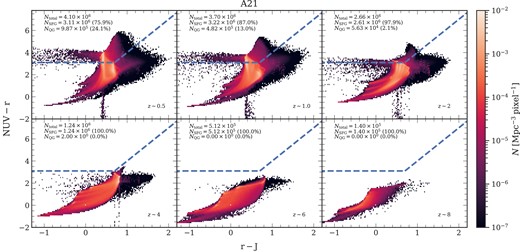
|$\rm NUVrJ$| colour–colour plot: The plot, combined for MRI and MRII, illustrates the |$\rm NUVrJ$| colour–colour selection criteria used to classify galaxies as either star-forming or quiescent across various redshifts. The classification is based on rest-frame |$\rm NUV-r$| and |$\rm r-J$| colours, following the methodology outlined by Ilbert et al. (2013) (blue dashed line). Galaxies above this relation are classified as quenched, while those below are considered star-forming. The number statistics for each redshift bin are also displayed in each subplot. Here, |${N_{\text{QG}}}$| represents the number of quiescent galaxies, and |${N_{\text{SFG}}}$| represents the number of star-forming galaxies in each subplot separated as per the |$\rm NUVrJ$| criterion. Furthermore, |${N_{\text{total}}}$| is the total number of galaxies at the represented redshift. The fraction (in per cent) of quenched and star-forming systems per total number of galaxies at each redshift is shown in the brackets. The plot shows the results from A21, and the results from H15 are given in Fig. A1.
Additionally, Fig. 3 serves as a consistency check, displaying the sSFRs for the |$\rm NUVrJ$| selected QG population in A21 (see Fig. A2 for H15). The 2D histogram is normalized by the sum of each column, so the colour coding represents the fraction of galaxies in each mass bin of size 0.14 dex with a pixel size of |$0.14 \:[\log ({\rm M}_{\odot })] \times 0.29 \:[\log ({\rm yr}^{-1})]$|. The histogram on the right axis shows the probability distribution function (PDF) of the sSFR at each redshift. Cells with |${\rm sSFR} \lesssim 10^{-12}$| are binned as a single column, because it is not normally possible to detect residual star formation in galaxies below this level.
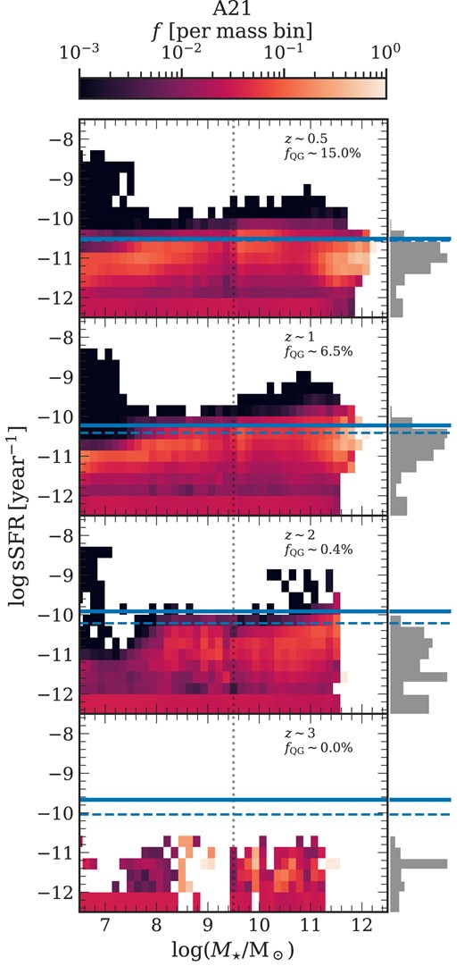
|${\rm sSFR}-M_\star$| plot for QGs: The plot illustrates the occupation of the |${\rm sSFR}-M_\star$| plane by the |$\rm NUVrJ$| selected QGs across different redshifts produced by A21. Two lines delineate the threshold sSFR values used to distinguish QGs from star-forming ones: the dashed line represents the sSFR cut-off according to Franx et al. (2008), while the solid line reflects the threshold from Henriques et al. (2020). The 2D histogram is normalized by the sum of each column, and the colour bar represents the fraction of galaxies per mass bin, with a bin width of 0.14 dex. In each subplot, |$f_{\text{QG}}$| represents the fraction (in per cent) of quiescent galaxies, for the whole mass range, above the Henriques et al. (2020) threshold. These are ‘falsely’ identified quenched systems by equation (4) having a high sSFR. The vertical grey dashed line separates the two boxes of the simulation at |${M_\star = 10^{9.5}\:{\rm M}_{\odot }}$| and cells with |${\rm sSFR} \lesssim 10^{-12}$| are binned as a single column. The grey histogram on the right axis shows the probability density distribution of the sSFR. Results from H15 are shown in Fig. A2.
This figure also displays two time-dependent sSFR cuts, one from Franx et al. (2008) (dashed line), which selects QGs having a |${\rm sSFR}\lesssim 0.3/t_{{\rm H}(z=0)}$|2 and another from Henriques et al. (2020) (solid line), which selects QGs as 1 dex below of the main sequence given by |${\rm sSFR}=2\times (1+z)^2/t_{{\rm H}(z=0)}$|. Additionally, |${f}_{\text{QG}}$| represents the fraction of galaxies above the Henriques et al. (2020) threshold. These galaxies have a higher sSFR and thus are effectively star-forming systems which are ‘misclassified’ as quenched by the |$\rm NUVrJ$| criterion.
Although A21 exhibits a small fraction of these misclassified systems, their relatively low numbers do not compromise the unified methodology applied across the models and observations, ensuring the robustness of our results. Most of these galaxies above the threshold are found to be massive satellite galaxies. In contrast, the centrals are below the threshold. This fraction of galaxies above the threshold, |${f}_{\text{QG}}$|, also decreases sharply for |$z\gtrsim 1$|. The PDF further illustrates that the bulk of the distribution remains well below these thresholds. Parallel results from H15 display similar trends, as shown in Figs A1 and A2.
4.2 Evolution of global galaxy properties to very high redshift
Assessing the agreement of global galaxy properties between simulations and observations is a crucial first step for validating and refining cosmological models. In this section, we evaluate the global consistency of the three L-galaxies flavours against observations.
4.2.1 The stellar mass function
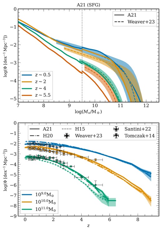
We calculate the SMF for the combined total sample of galaxies (SFGs and QGs) across five redshifts. To compute the SMF, at a given redshift, the number of galaxies within each 0.2 dex mass bin is divided by the volume of the corresponding simulation (MRI or MRII, detailed in Section 3.1) and is normalized by the bin width. The SMF is derived using a sliding bin approach with step size of 0.1 dex. Furthermore, we impose a minimum threshold of 20 galaxies per mass bin. If this threshold is not met, the bin size is increased by 0.1 dex iteratively until it is satisfied. Our primary point of comparison is with the findings of Weaver et al. (2023) (dashed lines), as presented in Fig. 4 (top) for A21 (see Fig. A3 for H15). We follow the mass completeness limits outlined by Weaver et al. (2023), incorporating their error estimates represented by shaded areas. The SMFs of the simulated galaxies are presented with solid lines, each accompanied by their respective one-sigma Poisson noise.
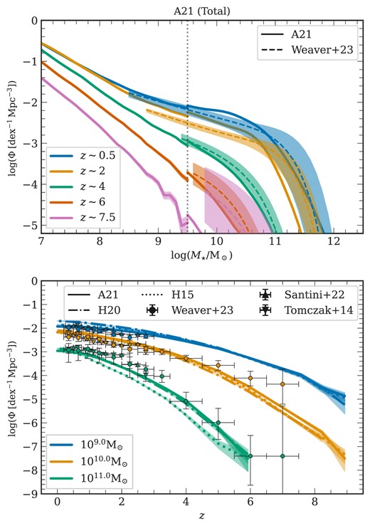
Total stellar mass function (top) and total galaxy number density as a function of redshift (bottom): In the top panel, the solid line shows the evolution of the stellar mass functions across five redshifts for the total (SFG and QG) galaxy sample from A21. The dashed line represents the observational findings from Weaver et al. (2023), with the accompanying shaded area indicating their errors. The total SMF from H15 are shown in Fig. A3. The bottom plot showcases the evolution of the number density of galaxies in three mass bins of 0.2 dex width as a function of redshift for the total galaxy sample. Each line style illustrates the results from distinct L-galaxies flavours: the solid line corresponds to A21, the dot-dashed to H20, and the dotted to H15. The coloured circular points mark the observational results from Weaver et al. (2023), Tomczak et al. (2014), and Santini et al. (2022), with the corresponding error bars indicated for each mass bin. In both plots, Poisson errors are represented by the similarly coloured shaded region. The data spans the mass range covered by the MRI and MRII simulations, subject to a transition region at |$M_\star = 10^{9.5}\:{\rm M}_{\odot }$|.
We note that the parameters of all the models were tuned to fit the stellar mass function at |$z=0$| as well as its evolution out to |$z=2$|. Model comparisons in the low redshift ranges do thus not represent a strong test of the input physics, so we will concentrate on higher redshift ranges in this paper. Comparisons for lower redshifts have been previously addressed in the respective publications detailing each model.
In Fig. 4 (top), the A21 flavour exhibits qualitative agreement in shape and evolutionary trends of the SMF across lower redshifts |$0\lesssim z \lesssim 2$|, albeit with small noticeable discrepancies. Similar to the findings in Weaver et al. (2023), we note that the SMF decreases monotonically with mass at |$z\sim 0.5 - 2$|. It tends to flatten out at lower redshifts before sharply falling at |$M_\star \sim 10^{11}\: {\rm M}_{\odot }$|. The simulation suggests that the slope of the low-mass end steepens into a power-law shape, whereas the high-mass end after the ‘knee’ falls off steeply, consistent with the finding of Weaver et al. (2023).
At high redshifts (|$z\gtrsim 2$|), a marked deficiency in high-mass galaxies (|$M_\star \gtrsim 10^{9.5}\:{\rm M}_{\odot }$|) is notable in all three flavours. The discrepancy between simulations and observations is most apparent at |$z\sim 2$| in all three flavours by displaying an excess of |$M_\star \lesssim 10^{10.8}\:{\rm M}_{\odot }$| galaxies and an underestimation of the SMF for more massive galaxies compared to observations. For even larger redshifts (|$z \gtrsim 5$|), the observations suggest a higher number density, but the growing uncertainty in the observational data complicates a clean separation of systematic errors and physical effects affecting the SMF’s shape.
In Fig. 4 (bottom), we illustrate the number density of galaxies per mass bin as a function of redshift categorized into three mass bins each spanning 0.2 dex. The line styles – solid, dashed, and dot-dashed – represent the different L-galaxies flavours, while the different markers indicate the observational data from Tomczak et al. (2014), Santini et al. (2022), and Weaver et al. (2023), along with their associated errors. These data points are derived from the corresponding Schechter function fits. Observational mass completeness limits are also depicted in this plot. The conclusions drawn from Fig. 4 (bottom) indicate subtle variations across the different L-galaxies flavours, with the H20 showing a slight excess of |$M_\star \sim 10^9 \: {\rm M}_{\odot }$| galaxies, a trend not observed in other flavours. Additionally, in all three models, there is a mild excess of |$M_\star \sim 10^{10} \: {\rm M}_{\odot }$| galaxies at cosmic noon (|$z\sim 2$|) and a slight deficiency of |$M_\star \sim 10^{11} \: {\rm M}_{\odot }$| galaxies at the same epoch, with H15 underestimating the number density in this heaviest mass bin. The models also show different growth rates of the most massive and least massive mass bins, consistent with the data. Overall, the A21 flavour offers improved performance across the three mass bins and redshifts, motivating the choice of this model as the fiducial model in this paper.
The evolution of the SMF indicates that the early universe predominantly contained small galaxies and that high-mass galaxies have not yet assembled. We observe a substantial mass buildup of approximately |$10^4\,\, [{\rm dex}^{-1}\:{\rm Mpc}^{-1}]$| between |$2 \lesssim z \lesssim 6$| for |$M_\star \sim 10^{11} \:{\rm M}_{\odot }$| galaxies, and about |$10^5 \,\,[{\rm dex}^{-1}\:{\rm Mpc}^{-1}]$| between |$2 \lesssim z \lesssim 8$| for |$M_\star \sim 10^{10} \:{\rm M}_{\odot }$| galaxies. Conversely, the number density appears to plateau at low-z for all three mass bins, suggesting a slow down in star formation. The turnover point in the SMF at around the Milky Way mass (|$M_\star \sim 10^{10.8}\:{\rm M}_{\odot }$|), above which the number density of galaxies sharply declines, provides critical insights into the efficiency of galaxy mergers and the feedback mechanisms from SN and AGN (e.g. Graham & Sahu 2023).
4.2.2 Evolution of the cosmic star formation rate density
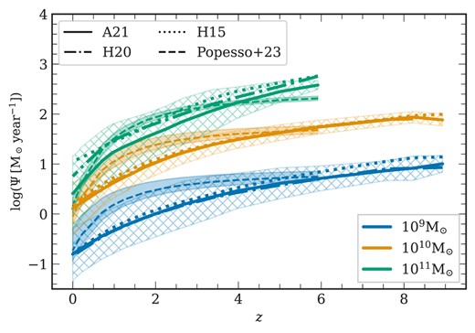
In Fig. 5, we compare the cosmic SFR density (CSFRD) in the three L-galaxies flavours with observational data from Bouwens et al. (2012), Madau & Dickinson (2014), Driver et al. (2018), Bouwens et al. (2020), Donnan et al. (2023), and Harikane et al. (2023), accompanied by the fits provided by Madau & Dickinson (2014) and Harikane et al. (2022). The SFRs of all galaxies are summed up and normalized by the volume of the corresponding box (detailed in Section 3.1). We convert all results from the Salpeter (1955) IMF to the Chabrier (2003) IMF using the conversion |$M_{\star ,{\rm Chabrier}}=0.64\times \,\,M_{\star ,{\rm Salpeter}}$|.
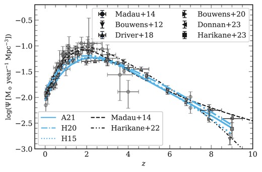
Cosmic SFR density as a function of redshift: The results from the different L-galaxies flavours are shown in different line styles in cyan. The observational data are obtained from Bouwens et al. (2012), Madau & Dickinson (2014), Driver et al. (2018), Bouwens et al. (2020), Donnan et al. (2023), and Harikane et al. (2023). The black dashed line and the dot-dot-dashed line are from Madau & Dickinson (2014) and Harikane et al. (2022), respectively, representing the observational fits.
While all three L-galaxies flavours exhibit a good qualitative agreement with the data between |$z\lesssim 1$| and |$2.5\lesssim z \lesssim 10$|, it is noteworthy that they tend to underestimate the CSFRD by approximately 0.15 dex, particularly at cosmic noon (|$1.5 \lesssim z \lesssim 2$|) when compared with the fit from Harikane et al. (2022). This underestimation coincides with significant discrepancies in the stellar mass functions (see Fig. 4), suggesting a potential decrease in star formation efficiency possibly due to inhibited gas cooling or insufficient gas density to sustain star formation. At the high-z end, L-galaxies agrees well with the results of Harikane et al. (2022) while having a steeper slope compared to Madau & Dickinson (2014), suggesting rapid galaxy mass buildup with a reasonably constant star formation efficiency (Harikane et al. 2022, 2023). Among the model flavours, H15 and H20 exhibit a slightly better agreement with the observed data, whereas A21 shows a suppression in the CSFRD at lower redshift (|$z\lesssim 2$|).
4.3 Evolution of the star-forming galaxy population
Similarly to the previous section, we calculate the SMF for the SFG sample separated using the |$\rm NUVrJ$| criterion (equation 4) and show the results in Fig. 6 (top). The SMF is plotted using a bin width of 0.2 dex, with a sliding step size of 0.1 dex and a minimum requirement of 20 galaxies per mass bin. We compare the simulation results with the observational findings of Weaver et al. (2023) including their one-sigma errors represented as the shaded regions.
Stellar mass function of SFGs (top) and SFG number density as a function of redshift (bottom): Similar to Fig. 4, the top panel depicts the SMFs for the sample of SFGs at four redshifts for the A21 flavour. The SMF from the H15 flavour is shown in Fig. A3. The bottom panel shows the galaxy number density per mass bin to redshift relation for the sample of SFGs in all three flavours along with the observed data.
The comparison between observations and simulations of the SFG SMF reveals similar discrepancies as those identified in the total SMF (see Fig. 4, top panel). At |$z\sim 2$| all three flavours display a lower turnover mass in the SFG SMF – |$10^{10.8}\,\,{\rm M}_{\odot }$| compared to the observed turnover at about |$10^{11.1}\,\,{\rm M}_{\odot }$|. This trend persists at other low redshifts. At larger redshifts (|$z\sim 5.5$|), all model flavours underestimate the abundance of star-forming systems. Furthermore, H15 exhibits a deficiency of SFGs with |$M_\star \gtrsim 10^{10.6} \:{\rm M}_{\odot }$| around |$z\sim 4$|, a limitation not observed in A21 or H20.
Overall, the SMFs of SFGs present varying shapes across different epochs, reflecting a double Schechter-like profile between |$0\lesssim z \lesssim 1.5-2$| with a ‘knee’ (characteristic mass) between |$M_{\star }\sim 10^{10.5}-10^{11.3} \: {\rm M}_{\odot }$|, which transitions to a power-law-like feature with a steep slope by |$z\sim 3$|.
In Fig. 6 (bottom), we show the redshift evolution of the number density per mass bin of SFGs compared to observational data from Tomczak et al. (2014), Santini et al. (2022), and Weaver et al. (2023). The simulations slightly overpredict the number density of low mass |$M_{\star }\sim 10^{9} \:{\rm M}_{\odot }$| systems at |$z\sim 2$| by about 1.5 times, and underpredict the massive |$M_{\star }\sim 10^{11} \:{\rm M}_{\odot }$| systems at |$z\gtrsim 3$| by a factor of 2. For |$M_{\star }\sim 10^{10} \:{\rm M}_{\odot }$| systems, an excess of simulated galaxies is seen at cosmic noon (|$1.5 \lesssim z \lesssim 2$|). This could be an indication of incompleteness or biases in the observations suggesting a non-physical origin (Ilbert et al. 2013; Weaver et al. 2023).
Among the model flavours, A21 agrees best with the observational data, whereas H20 tends to overestimate the numbers in the low mass bins and H15 underestimates the high mass bins by about 0.2 dex. This plot further illustrates the rapid mass assembly of massive galaxies through mergers, while lower mass galaxies exhibit a slower, more gradual increase in number density across cosmic epochs. We note a moderate growth of SFGs of about 1.5 times since |$z\sim 2$|, while a growth by about a factor 15 is observed for |$M_{\star }\sim 10^{10}\: {\rm M}_{\odot }$| galaxies from |$2\lesssim z \lesssim 4$|. The most massive galaxies grow by a factor of 40 over the same redshift range. The differences between the simulations and the observations underscore potential issues in the galaxy quenching mechanisms. Our results also demonstrate that the discrepancies with the data seen in the SMF arise from the star-forming population, which dominates the total population by number across the entire redshift range (see Fig. 2).
4.4 Evolution of the quiescent galaxy population
As described in Section 4.1, the selection of QGs is based on the |$\rm NUVrJ$| criterion (equation 4). The QG SMF for A21 is presented in Fig. 7 (see Figs A3 and A4 for the results of H15 and H20). It is derived similarly to the method described in Section 4.2.1, and a comparison is made with the observational results of Weaver et al. (2023) including the quoted errors. The SMFs outside of the |$M_\star =10^{9.5}\:{\rm M}_{\odot }$| transition threshold of the MRI and MRII simulations are represented as fainter lines, highlighting the convergence of the two runs. This shows good agreement at |$z\sim 0.5$|, although the quality of the alignment degrades at higher redshifts.
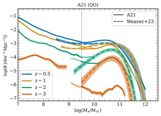
Stellar mass function of QGs: This figure displays the QG SMF at four different redshifts within the A21 flavour alongside observational fits from Weaver et al. (2023). Simulation results from MRI for |$M_\star \lesssim 10^{9.5}\:{\rm M}_{\odot }$| and MRII for |$M_\star \gtrsim 10^{9.5}\:{\rm M}_{\odot }$| are presented using fainter solid lines to indicate the transition region between the two runs (refer to Section 3.1). The results from the other L-galaxies flavours are shown in Figs A3 and A4.
The three L-galaxies model flavours achieve reasonable agreement with the observed low-redshift (|$z\lesssim 2$|) QG SMF with small 0.1–0.2 dex deviations, reproducing the double Schechter function appearance noted by e.g. Santini et al. (2022). Note that the ‘knee’ of the SMF – the point marking a significant downturn in the number density of galaxies – occurs at a slightly lower mass in the simulations compared to observations. At redshifts, |$z\sim 0.5 - 1$|, the discrepancy between the ‘knee’ of the SMF in observations and simulations is about |$0.3-0.4$| dex. While A21 reproduces a double Schechter-like profile, including a characteristic upturn at lower masses due to updated environmental effects, this feature is less pronounced in H20 and absent in H15. In A21, the double Schechter function-like shape is also seen at larger z, suggesting that the updated prescription for environmental effects is important for producing the population of quenched low-mass galaxies. However, at |$z\gtrsim 2$|, the observational data may suffer from incompleteness issues, leading to an exponential decline in the QG SMF at lower masses (|$M_\star \lesssim 10^{10}\:{\rm M}_{\odot }$|). This contrasts with the mass buildup observed in low-mass quenched systems in the A21 model flavour, also aligning closely with some observational findings (e.g. Santini et al. 2022).
A notable deficit of QGs is evident in all three L-galaxies flavours at |$z\gtrsim 2$|. Fig. 8 presents a more detailed exploration of the evolution of the quiescent galaxy population, with the simulated galaxy population decomposed into contributions from central and satellite galaxies. The evolution of the QG number density per mass bin is shown in a series of mass bins, each 0.2 dex wide, as a function of redshift. Here, centrals are marked in black and satellites in purple, with the cross-hatched region indicating one-sigma Poisson errors. Different line styles are used for the different L-galaxies flavours. Observational data from Tomczak et al. (2014), Santini et al. (2022), and Weaver et al. (2023) with their errors and mass completeness limits are also shown. It is important to note that Weaver et al. (2023) quote large error bars at |$z \gtrsim 4$| due to mass incompleteness, observing only 200 quenched systems in this regime and only 1 object at |$z\sim 6$|, which limits confidence in their SMF fit to the range |$3.5 \lesssim z\lesssim 4.5$|.
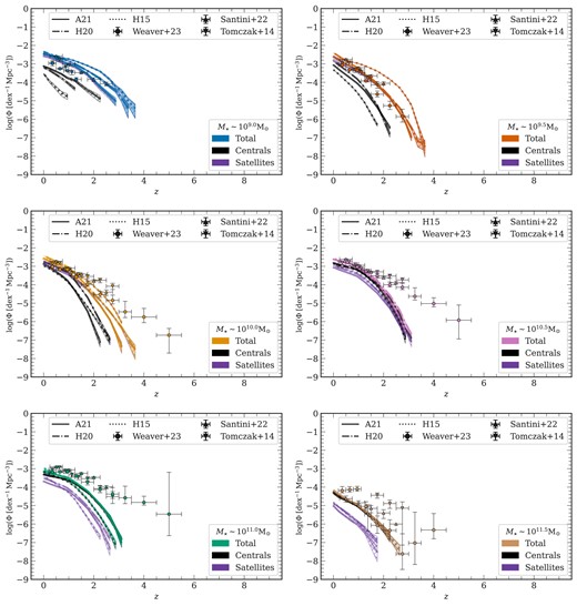
QG number density as a function of redshift: Similar to Figs 4 and 6, these panels depict the galaxy number density per mass bin as a function of redshift for the sample of QGs for the three model flavours. The plot is divided into six panels representing the six mass bins from |$10^{9}\:{\rm M}_{\odot }$| to |$10^{11.5}\:{\rm M}_{\odot }$|, with each mass bin having a width of 0.2 dex. In each plot, the number density of QGs is then split for centrals and satellites represented in black and purple, respectively. The simulation results are also shown with one-sigma Poisson errors. It includes the corresponding observational data points and errors from Tomczak et al. (2014), Santini et al. (2022), and Weaver et al. (2023).
There is a slight excess of the lowest mass galaxies in the simulations at all redshifts in all three L-galaxies model flavours. A similar discrepancy was noted by Harrold et al. (2024) when comparing L-galaxies predictions to UKIDSS Ultra-Deep Survey data (UDS; Lawrence et al. 2007). The excess found in our work is smaller.
We note that satellite galaxies are the dominant contributors to the number density of very low mass QGs at all redshifts, whereas central QGs become more prevalent in the higher mass bins. The dominance of centrals over satellites occurs at |$M_\star \approx 10^{10.2}-10^{10.3}\: {\rm M}_{\odot }$| in the models.
In the intermediate mass bins of |$M_\star \sim 10^{10}\: {\rm M}_{\odot }$| and |$M_\star \sim 10^{10.5}\: {\rm M}_{\odot }$|, the simulation results align well with the observations at lower redshifts (|$z\lesssim 2-2.5$|). At higher redshifts, the number density of simulated QGs decreases more rapidly than observed.
In the high mass bin (|$M_\star \sim 10^{11} \:{\rm M}_{\odot }$|), there is a considerable shortfall in the number density of simulated QGs relative to observations, with the gap widening to a factor of 60 by |$z\approx 3$|. In this range, massive quenched centrals are the primary contributors. The final mass bin (|$M_\star \sim 10^{11.5} \:{\rm M}_{\odot }$|) suffers from large variability in the observational data, and a precise conclusion is difficult to draw. Nevertheless, the number density of quenched galaxies is often underpredicted in the L-galaxies simulations.
The results presented in this section suggest potential model limitations in capturing early quenching processes. The dominance in these plots shifts from satellites to centrals around |$M_\star \sim 10^{10.2}-10^{10.3}\: {\rm M}_{\odot }$|, coinciding with the proposed critical mass threshold for ‘mass quenching’ suggested by Peng et al. (2010b). This threshold delineates where the influence of a galaxy’s own properties such as mass and black hole activity outweigh external factors such as environmental effects or interactions with other galaxies.
In summary, the QG SMF offers valuable insight into the evolution of quenched systems across different epochs. In the three L-galaxies flavours, we observe a rapid evolution and significant mass buildup in massive quenched centrals starting from |$z \sim 3$|, a rate much faster than what observations suggest. Observational data generally indicate a milder evolutionary slope for these large mass bins (|$M_\star \sim 10^{10}-10^{11}\:{\rm M}_{\odot }$|). Conversely, in the lower mass bins predominantly comprised of satellites, there is an overabundance of QGs, with the degree of this surplus varying depending on the observational data set adopted. We note that because lower mass galaxies have lower surface brightnesses, corrections for selection effects are more difficult and thus our comparison for this specific mass range may not be as robust as for the more massive systems.
Finally, a crucial point that we find in our analysis is the complete absence of massive quenched systems beyond |$z \sim 3-3.5$| in the models. This could introduce a significant challenge to the implementation of physical processes in our galaxy formation models.
4.5 Evolution of the star-forming main sequence
The main sequence of star-forming galaxies is illustrated in Fig. 9 for A21. The plot presents a 2D histogram representing the simulated galaxies in the |${\rm SFR}-M_\star$| parameter space normalized by the respective volume (MRI or MRII, see Section 3.1), thus the colour coding suggests the density of galaxies per cubic Mpc per pixel of size |$0.18\: [\log ({\rm M}_{\odot })] \times 0.33\:[\log ({\rm M}_{\odot }\,{\rm yr^{-1}})]$|. The solid blue line traces the running mean of the distribution, while the blue cross-hatched region represents the one-sigma scatter around the mean. A comparison is made to the findings of Popesso et al. (2023) using the fitting function of Lee et al. (2015), shown by the solid yellow line, and Speagle et al. (2014) is represented by the red line. The shaded regions around these lines indicate the quoted errors. Additionally, we account for the IMF offset in both Speagle et al. (2014) and Popesso et al. (2023), and convert the Kroupa (2001) IMF to a Chabrier (2003) IMF using the relation |$M_{\star ,{\rm Chabrier}}=0.94 \times M_{\star ,{\rm Kroupa}}$|.
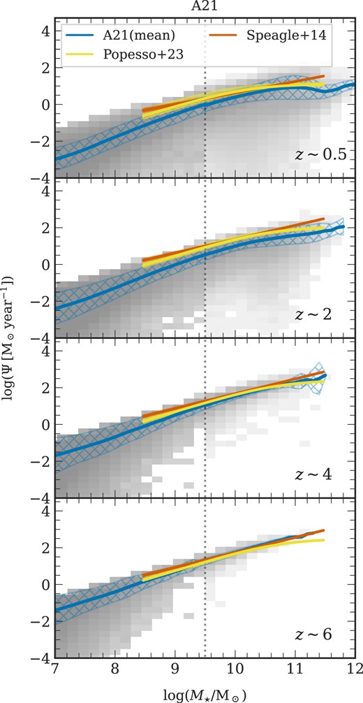
|${\rm SFR}-M_\star$| relation: A plot describing the main sequence of star-forming galaxies across various redshifts for the A21 flavour. The yellow line represents the observational fit from Popesso et al. (2023), with its uncertainty indicated by the surrounding yellow shaded area, while the red line depicts the relation from Speagle et al. (2014) with its errors. The grey-shaded region in each plot denotes the distribution of galaxies from A21. Additionally, the solid blue line traces the running mean in the mass bin of the simulated galaxies. The blue cross-hatched region represents the one-sigma scatter from the mean. The results from other flavours are shown in Fig. A5.
The three model flavours align well within one-sigma scatter with Speagle et al. (2014) across all masses and redshifts (for results from H15, see Fig. A5). In A21, particularly for |$0\lesssim z\lesssim 4$|, where the SFR is observed to plateau at higher masses near the turnover mass (|$\sim 10^{10.5}\:{\rm M}_{\odot }$|), the SFR is suppressed and remains nearly constant for larger masses, while below this mass, the SFR is proportionally increasing with stellar mass. This is consistent with findings from Popesso et al. (2023) suggesting a flattening at the high-mass end. This flattening trend, while absent in H15, is less pronounced in H20 at lower redshifts and is also absent in A21 at larger redshift (|$z\gtrsim 5$|). The observed flattening at high-z, as reported by Popesso et al. (2023), suggests a decrease in star formation efficiency at higher masses. This likely reflects the cumulative effects of less efficient gas cooling and increased feedback mechanisms in massive galaxies, or it could be attributed to the transition in halo mass from predominantly cold to hot gas accretion (Dekel & Birnboim 2006).
More obvious discrepancies between the models and the data can be seen in Fig. 10, which shows the SFR as a function of redshift for three mass bins of 0.2 dex width. In this plot, we show results for all three L-galaxies flavours. The cross-hatched markings represent one-sigma scatter from the mean SFR of the A21 flavour.
SFR to redshift relation: A plot showing the evolution of SFR as a function of redshift in three different stellar mass bins, colour-coded accordingly with a bin width of 0.2 dex. The line style indicates the results from different L-galaxies flavours: the solid line corresponds to A21, the dot-dashed line to H20, and the dotted line to H15. Additionally, the dashed line represents the observational findings from Popesso et al. (2023), with the corresponding uncertainties depicted by the shaded regions. The cross-hatched region represents the one-sigma scatter from the mean for each mass bin, applicable only for the results from A21.
We note a reasonably good agreement with the work of Popesso et al. (2023) for all the mass bins for the three flavours, although there are some discrepancies. At lower redshift (|$z \lesssim 0.5-1$|), the models align well for the |$M_\star \sim 10^{9}\: {\rm M}_{\odot }$| and |$M_\star \sim 10^{10}\: {\rm M}_{\odot }$| bins. However, the mean SFR for the |$M_\star \sim 10^{11}\, {\rm M}_{\odot }$| bin tends to be overpredicted by H20 and H15, and to a lesser degree in A21. At higher redshifts (|$z \gtrsim 4$|), all three flavours overpredict the SFR of the highest mass bin. This suggests that the model’s predictions for the SFR of high-mass galaxies need to be further suppressed to match the observed trends at the higher redshifts more accurately.
For the least massive |$M_\star \sim 10^{9}\:{\rm M}_{\odot }$| galaxies, all three models deviate from the results of Popesso et al. (2023) over the redshift range |$0.5 \lesssim z \lesssim 4$|, with the SFRs in the models lying a factor of |$2-3$| below the observations. This result echoes the broader discrepancy seen in Fig. 5 for the integrated CSFRD. The main conclusion from the |${\rm SFR}-M_\star$| comparison is that the lower mass galaxies are responsible for the offset between the data and the models. For the redshift range from |$0.5 \lesssim z \lesssim 4$| and all three mass bins, the models underpredict the mean SFR, once again suggesting that revisions in the implementation of physical processes relevant to star formation and quenching are necessary to align more closely with the observations.
4.6 Evolution of galaxy mass–size relation
Estimating galaxy sizes is typically done via one of two methods: aperture fluxes, also known as the curve of growth (CoG) approach (e.g. Carollo et al. 2013), or profile fitting (e.g. der Wel et al. 2014a). In the L-galaxies model, the half-light radii or the effective radii (|$R_{\rm e}$|) can be calculated only for two flavours, namely H20 and A21, as these models contain resolved properties of galaxies (see Section 3.2). Both of these flavours employ the CoG, which iteratively determines the radius encompassing half of the total flux of the galaxy. In contrast, the work of der Wel et al. (2014a) and Mowla et al. (2019) uses a Sérsic profile fit (Sérsic 1963) to derive this property from the observations. It is worth noting that both approaches are susceptible to systematic biases in estimating |$R_{\rm e}$| (e.g. Shen et al. 2003; Graham et al. 2005; Cameron & Driver 2007; Whitaker et al. 2011; Ichikawa, Kajisawa & Akhlaghi 2012; der Wel et al. 2014a).
Due to the availability of resolved data for galaxy properties in H20 and A21, we derive the surface brightness profiles of each galaxy and fit a single-component 1D Sérsic profile to obtain |$R_{\rm e}$| in the rest-frame V (|$0.55 \: \mu {\rm m}$|) band filter, using a surface brightness limit |$I_{\rm limit} = 26.6 \,\, [{\rm mag}\,\, {\rm arcsec}^{-1}]$| (Papovich et al. 2012) (more details in Appendix C), consistent with the observational data from der Wel et al. (2014b) and Mowla et al. (2019). This allows for a comparison between |$R_{\rm e}$| estimates from the CoG approach and those from the Sérsic profile fit as well.
In Fig. 11, we present the galaxy mass–size relation for SFGs (left) and QGs (right) in the A21 flavour. Each panel includes data from different redshifts and displays a 2D histogram representing |$R_{\rm e}$| derived from the CoG approach (|$R_{\rm e, CoG}$|), with the solid blue line and the cross-hatched region showing the running mean and the scatter, respectively. The colour coding of the 2D histogram illustrates the number density of galaxies per cubic Mpc per pixel of size |$0.18\: [\log ({\rm M}_{\odot })] \times 0.10\:[\log ({\rm kpc})]$|. The dashed blue line represents the half-mass radius, |$R_{\rm hm}$|, defined as the radius encompassing half of the galaxy’s stellar mass. Additionally, the blue dot-dashed line shows |$R_{\rm e}$| derived from the Sérsic fit (|$R_{\rm{e, S'{e}rsic}}$|) accompanied by the plus-hatched region depicting its one-sigma scatter from the mean. The Sérsic fit results from the model can be compared directly with observational relations from der Wel et al. (2014a) and Mowla et al. (2019). The solid red line represents parametrized fits from the work of der Wel et al. (2014a), measured along the semimajor axis of an ellipse, with the respective one-sigma scatter along the mean. The left vertical axis is in log units while the right axis of the plots is shown in linear kpc units.
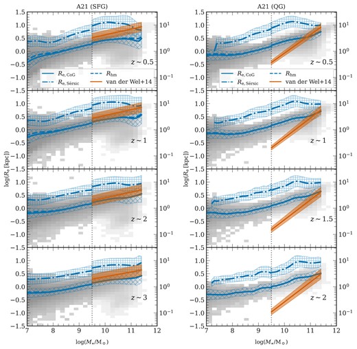
Galaxy mass–size relation: The plots illustrate the |$R_{\rm e}-M_\star$| relation, specifically the half-light radii denoted as |$R_{\rm e}$|, the radius encompassing half of the total flux of the galaxy. This relation is plotted for the SFGs (left) and QGs (right) at four redshifts for the A21 model flavour. The 2D histogram shows the distribution of |$R_{\rm e,\:CoG}$| of simulated galaxies, with the solid blue line tracing the mean of the distribution. The blue dashed line represents the half-mass radius (|$R_{\rm hm}$|). In the L-galaxies model, |$R_{\rm e}$| is derived in two ways: using the curve of growth approach (|$R_{\rm e,\:CoG}$|, solid blue line) and by fitting a 1D Sérsic profile (|$R_{\rm{e, S'{e}rsic}}$|, dot-dashed blue line). The blue cross-hatched and plus-hatched region represents the one-sigma scatter around |$R_{\rm e,\:CoG}$| and |$R_{\rm{e, S'{e}rsic}}$|, respectively. The red line corresponds to the relation by der Wel et al. (2014a) with one-sigma scatter. The right axis of the plot is in linear units. Mass incomplete measurements of der Wel et al. (2014a) are not shown.
In the left panel of Fig. 11, representing SFGs of A21, the solid blue line indicates a strong correlation of |$R_{\rm e, CoG}$| with stellar mass until |$M_\star \sim 10^{10.5}\:{\rm M}_{\odot }$|, after which the relation flattens. The flattening is stronger at lower redshifts. The dot-dashed line, representing the Sérsic fit half-light radius (|$R_{\rm{e, S'{e}rsic}}$|), shows a similar flattening at high stellar masses.
Overall, the galaxy sizes predicted by the model are larger than the observed sizes. The discrepancy is largest for QGs and for low-mass galaxies (Fig. 11right panel). At stellar masses of |$M_\star \sim 10^{9.5} {\rm M}_{\odot }$|, the size discrepancies in the quenched population reaches a factor of 10 at low redshifts (|$z\sim 0.5$|) and nearly a factor of 30 at |$z\sim 2$|. The agreement between the models and the observations is best for high-mass star-forming galaxies. The size–mass relation over the stellar mass range |$10^{9.5}-10^{11} \: {\rm M}_{\odot }$| is considerably flatter in the models than in the observations. The discrepancy in the slope of the relation is again worse for the quiescent population.
In Fig. 12, the evolution of galaxy sizes as a function of redshift is shown in three different mass bins. The solid and dot-dashed lines represent the mean |$R_{\rm e}$| of the two flavours from the CoG approach while the sparsely spaced dashed line and the dotted line show the values derived using the Sérsic fit. Each colour corresponds to a specific mass bin, each having a 0.2 dex bin width. Additionally, the markers represent the observational data points from der Wel et al. (2014a) and Mowla et al. (2019).
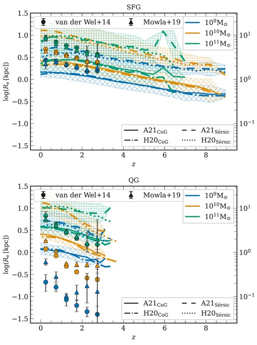
Galaxy size to redshift evolution: These figures illustrate the evolution in |$R_{\rm e}$| as a function of redshift for three mass bins of 0.2 dex bin width for the SFG sample (top) and QG sample (bottom). The solid and dot-dashed lines represent the results from A21 and H20, respectively, using the curve of growth (CoG) approach with the cross-hatched region denoting one-sigma scatter for the results of A21. The dashed and dotted lines represent the results from A21 and H20, respectively, for |$R_{\rm e}$| derived from the 1D Sérsic fit, with the plus-hatched region denoting scatter in the results of A21. The results are compared with the data from der Wel et al. (2014a) and Mowla et al. (2019).
The results shown in the top panel of Fig. 12 indicate that the A21 and H20 models both predict a mild evolution of |$R_{\rm e}$| for SFGs. However, the model results do not match the observations in detail, displaying a size discrepancy of approximately a factor of |$1.5-2$|. The offset between sizes derived by the two methods is also evident in the plots. Despite this, a general agreement with the slope of |$R_{\rm e}$| as a function of z is observed for stellar mass bins |$10^{9}\:{\rm M}_{\odot }$|, |$10^{10}\:{\rm M}_{\odot }$|, and |$10^{11}\:{\rm M}_{\odot }$| when considering |$R_{\rm e}$| derived from the Sérsic fit.
Fig.12 (bottom), illustrates the evolution for QGs, and reveals a noticeable discrepancy in the size evolution of galaxies between the model and the data. The very steep evolution suggested by observations is not replicated in the models. Although there seems to be some consistency and agreement in the largest mass bin |$M_\star \sim 10^{11}\:{\rm M}_{\odot }$| for the sizes derived by the CoG approach (solid and dot-dashed lines), the agreement with data is much worse for the lower mass bins. Overall, the discrepancy detected between the sizes of simulated and observed galaxies is typically larger for QGs than for star-forming galaxies. This could reflect the complex set of physical processes related to size evolution such as mergers (Naab et al. 2009), host dark matter halo properties (Zanisi et al. 2020), or the distribution of stars within galaxies (Dabringhausen, Hilker & Kroupa 2008; Vera-Ciro et al. 2014; Grand, Kawata & Cropper 2015; Okalidis et al. 2022)
4.7 Evolution of the central surface mass density
With resolved data from the L-galaxies simulations, we can derive stellar mass surface densities within a 1 kpc radius (core) or the effective radius (|$R_{\rm e}$|, see Section 4.6 and Appendix C), by utilizing the model flavours with radial rings, i.e. A21 and H20. The surface mass densities include the stellar mass contribution from the bulge and the disc.
As outlined in Section 2.5, QGs should be characterized by higher |$\Sigma _{1\,\,{\rm kpc}}$|, but this is only weakly seen in Fig. 13 for A21. Both L-galaxies flavours exhibit a tight correlation between the galaxy stellar mass and |$\Sigma _{1\,\,{\rm kpc}}$|. Fig. 13 presents simulation data from A21 for the SFGs (left) and QGs (right), with the 2D histogram illustrating the distribution of stellar mass surface densities simulated galaxies while the colour coding representing the median Sérsic index of each pixel of size |$0.18\: [\log ({\rm M}_{\odot })] \times 0.15\:[\log ({\rm M}_{\odot }\:{\rm kpc}^{-2})]$|. The blue line and the cross-hatched region show the running mean of the distribution and its one-sigma scatter. The observational results from Barro et al. (2017) are plotted with a red line, including a one-sigma scatter and mass completeness limits. Both SFGs and QGs in the model flavours align well with observed data, showing similar trends and evolution. However, intermediate mass (|$M_\star \sim 10^{10}\:{\rm M}_{\odot }$|) quenched systems are not as compact as noted in the observations.
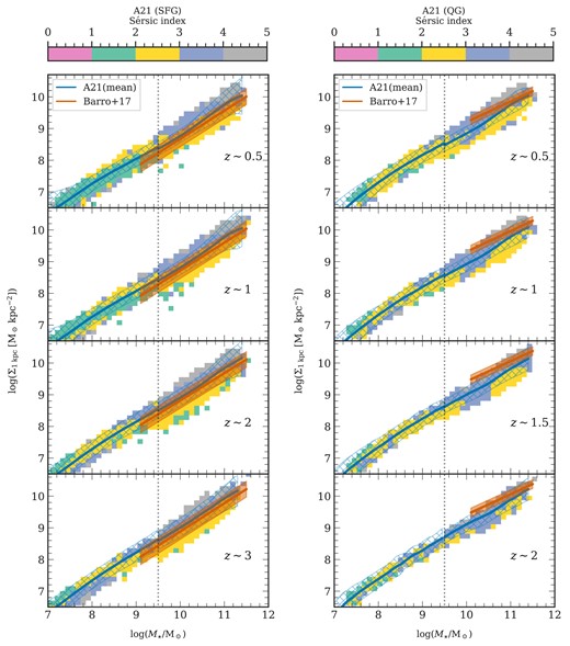
Galaxy core stellar mass surface density to mass relation: The plots illustrate the core (|$R\lt 1\,\,{\rm kpc}$|) stellar mass surface density to galaxy mass relation for the SFG (left) and the QGs (right) at four redshifts presented for A21. The 2D histogram shows the distribution of simulated galaxies with the blue line tracing the running mean and the blue cross-hatched region denoting the one-sigma scatter around the mean. The colour indicates the median Sérsic index of each mass bin, shown if the fit is within 10 per cent of the residuals. The red line represents the relation derived from Barro et al. (2017) along with one-sigma scatter around the mean represented as the shaded region.
The Sérsic index (n) for galaxies is shown in the two plots only if the residual3 of the single-component 1D Sérsic fit is less than 0.1, suggesting the fits are considered good within a 10 per cent threshold. The scatter with high Sérsic indices in the surface density–stellar mass plane lies outside the 1-sigma scatter represented by the cross-hatched region of the solid blue line and includes only a negligible number of galaxies. This index n (detailed in Appendix C), presents higher values in both SFGs and QGs within A21 and H20 compared to those reported by Barro et al. (2017). Typically, QGs (Figs 13, 14, right panels) exhibit higher Sérsic indices than their star-forming counterparts, correlating with their more compact nature. The complex shape of surface brightness profiles and the notably high Sérsic indices reported here underline the limitations of using a single component 1D Sérsic fit. This mismatch suggests that a single-component Sérsic profile may not effectively capture the structural differences of these galaxies.
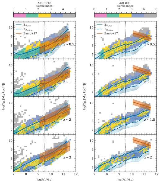
Galaxy effective stellar mass surface density to mass relation: Similar to Fig. 13 the plot represents the stellar mass surface densities within one effective radius (|$\Sigma _{R_{\rm e}}$|). The relation is shown for the SFGs (left) and QGs (right) for the A21 flavour. In the L-galaxies model, |$R_{\rm e}$| is derived in two ways: using the curve of growth approach (|$\Sigma _{ R_{\rm e,\:CoG}}$|, solid blue line) and by fitting a 1D Sérsic profile (|$\Sigma _{R_{\rm{e, S'{e}rsic}}}$|, dot-dashed blue line). The blue plus-hatched region represents the one-sigma scatter around |$\Sigma _{R_{\rm{e, S'{e}rsic}}}$|, while the cross-matched region is for one-sigma scatter around |$\Sigma _{R_{\rm e, CoG}}$|. The results from Barro et al. (2017) are plotted in red. The colour coding states the median Sérsic index of each mass bin if the Sérsic fit is within 10 per cent of the residuals.
Fig. 14 shows the |$\Sigma _{R_{\rm e}}-M_\star$| relationship with the mean Sérsic index denoted by the colour bar. The running mean of the |$\Sigma _{R_{\rm e, CoG}}$| values derived using the CoG approach is shown as the solid blue line, while the |$\Sigma _{R_{\rm{e, S'{e}rsic}}}$| values derived using the 1D Sérsic fit is shown as the dot-dashed blue line. The observational results from Barro et al. (2017) are shown in red. The SFGs are in good agreement with the observations for almost all masses. In contrast, the quenched systems diverge from the observed data, especially for the low mass |$M_\star \sim 10^{10}\:{\rm M}_{\odot }$| galaxies which appear significantly less compact deviating at most by a factor of 80 at all redshifts. The most massive |$M_\star \sim 10^{11}\:{\rm M}_{\odot }$| QGs display a flatter |$\Sigma _{R_{\rm e, CoG}}-M_\star$| relation at lower redshift, suggesting a better qualitative agreement with the observations.
Fig. 15 illustrates the redshift evolution of the stellar mass surface densities in three mass bins of 0.2 dex bin width. For the SFGs (Fig. 15, left column), the agreement with observational data is generally robust. The most massive star-forming systems, around |$M_\star \sim 10^{11}\:{\rm M}_{\odot }$| have stellar mass densities both within 1 kpc (|$\Sigma _{1\:{\rm kpc}}$|) and at effective radius (|$\Sigma _{R_{\rm e}}$|) that agree reasonably well with observations. The intermediate-mass star-forming systems of |$M_\star \sim 10^{10}\, {\rm M}_{\odot }$| agree well on the |$\Sigma _{1\:{\rm kpc}}-M_\star$| plane, though they appear about |$3-4$| times denser than observed within |$1\, R_{\rm e}$|. The lowest mass galaxies tend to be overdense in the simulations.

Galaxy core and effective stellar mass surface density to redshift evolution: This figure illustrates the evolution of the stellar mass surface density as a function of redshift for the SFG fraction (left column) and QG fraction (right column) in three mass bins (0.2 dex bin width) for two L-galaxies flavours. The upper panel shows the stellar densities with 1 kpc while the bottom panel shows the effective densities. In the upper panels, the solid line represents the data from A21, and the dot-dashed line represents the results from H20. The cross-hatched region denotes the scatter around the mean of the A21 results. For the effective densities, the solid and dot-dashed lines have used the curve of growth (CoG) approach to derive the |$R_{\rm e}$|, while the loosely dashed and dotted line use the Sérsic fit to find the |$R_{\rm e}$|, where the one-sigma scatter of A21’s Sérsic fit and CoG fit is shown with a plus-hatched and cross-hatched region, respectively. The markers are from Barro et al. (2017). The |$10^9\:{\rm M}_{\odot }$| mass bin is outside the completeness limits of Barro et al. (2017) for the quenched fraction, hence not included in the right column.
The quenched systems exhibit much worse inconsistencies with the data. As shown in Fig. 15 (right column), the most massive QGs agree with observed |$\Sigma _{1\:{\rm kpc}}$| densities, while those around |$M_{\star }\sim 10^{10}\:{\rm M}_{\odot }$| are significantly less dense – about 4 to 6 times lower than the values reported by Barro et al. (2017). |$\Sigma _{R_{\rm e}}$| densities exhibit a strong evolution in the densities of |$M_\star \sim 10^{10}\:{\rm M}_{\odot }$| and |$M_\star \sim 10^{11}\:{\rm M}_{\odot }$| galaxies. The intermediate-mass systems are about |$80-100$| times less dense than the observations. We note that there are uncertainties in the observational data due to poor statistics in the |$2.2\lesssim z\lesssim 3$| range.
The distribution of the Sérsic indices in the |$\Sigma _{1\:{\rm kpc}}-M_\star$| and |$\Sigma _{R_{\rm e}}-M_\star$| planes in the A21 and H20 models do not align with Barro et al. (2017)’s observations. Specifically, SFGs in our models show a lower Sérsic index (|$n \approx 1-2$|) for lower mass galaxies, indicating a disc-like structure, while more massive galaxies (|$M_\star \gtrsim 10^{10}\:{\rm M}_{\odot }$|) exhibit higher indices (|$n \approx 2-3$|), pointing to a bulge-dominated morphology. The highest mass galaxies (|$M_\star \gtrsim 10^{11}\:{\rm M}_{\odot }$|) in our simulation exhibit Sérsic indices greater than 4, further indicating a bulge-dominated structure. Moreover, in the |$\Sigma _{R_{\rm e}}-M_\star$| plane, while the median SFGs typically show |$n\approx 1-3$|, the range extends up to |$n\approx 4-5$| at the upper edge of the distribution, deviating from Barro et al. (2017)’s findings where SFGs in this plane with |$\log \Sigma _{R_{\rm e}} \gtrsim 9.5$| and |$M_\star \gtrsim 10^{10}\:{\rm M}_{\odot }$| are expected to have Sérsic indices between 2 and 4. Overall, QGs tend to show higher indices compared to the SFGs, with medians |$n\approx 2-3$|, underscoring their bulge-dominated nature. Our models demonstrate a broader spread of n, from approximately 1 to 5 for SFGs and 2 to 5 for QGs, suggesting a need for further refinement in modelling the structural parameters of galaxies.
5 BARYONIC PHYSICS CONTROLLING QUENCHING
The star formation rates of galaxies are controlled by a complex set of physical mechanisms that control the rate at which gas will cool and form stars in galaxies. In order to gain insight into the primary mechanisms responsible for galaxy quenching in the A21L-galaxies flavour, here we explore the distribution of baryons within haloes and investigate the relationship between quenching, black hole mass, hot gas mass, and cold gas mass in galaxies across different cosmic epochs.
5.1 Halo baryon and gas fractions
Fig. 16 displays the halo baryon and gas fractions in A21 across six different redshifts. The baryon fractions (|$f_{\rm b}$|) are calculated by summing up the contributions of all baryonic components within the virial radius (|$R_{200}$|)4 and dividing it by the virial mass (|$M_{200}$|).5 The resulting ratio is then normalized by the cosmic baryon fraction |$f_{\rm b, cosmic}=\Omega _{\rm b}/\Omega _{\rm m}\approx 0.16$| (Planck Collaboration XIII 2016). Similarly, the gas fractions (|$f_{\rm gas}$|) are calculated based on the combined contributions of hot and cold gas within each halo. The mean baryon and gas fractions are plotted with a one-sigma scatter from the mean, represented by the shaded region. A cut is applied to separate the MRI and MRII simulation results at |$M_{200}=10^{11.5}\:{\rm M}_{\odot }$|, analogous to the |$M_\star =10^{9.5}\:{\rm M}_{\odot }$|.
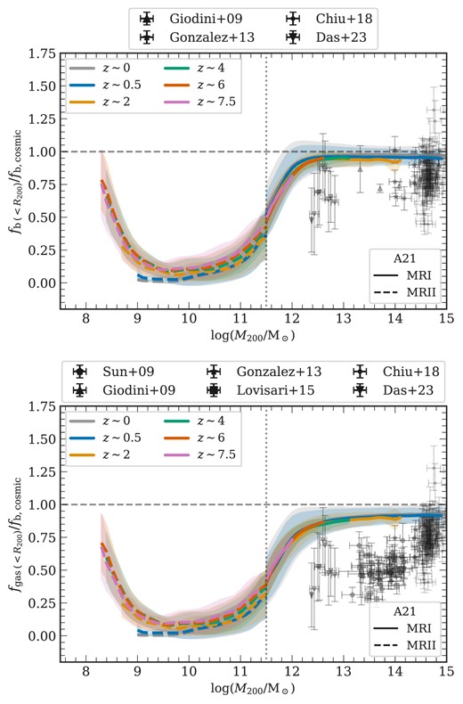
Halo baryon and gas fractions: The plot displays the distribution of baryon (top) and gas (bottom) fractions across different halo masses (|$M_{200}$|) for six redshift intervals. The solid and dashed lines represent the mean fractions from the MRI and MRII simulations, respectively, each normalized by the cosmic average and illustrated with a one-sigma scatter. The plot is also divided at |$M_{200}=10^{11.5}\:{\rm M}_{\odot }$|, equivalent to |$M_\star =10^{9.5}\:{\rm M}_{\odot }$| which separates the contribution of MRI from MRII. Observational data points at |$z\approx 0$| from Giodini et al. (2009), Sun et al. (2009), Gonzalez et al. (2013), Lovisari, Reiprich & Schellenberger (2015), Chiu et al. (2018) (within |$R_{500}$|), and Das, Chiang & Mathur (2023) (within |$R_{200}$|) are overlaid for comparison.
Observational measurements at |$z\approx 0$| of the baryon content within |$R_{500}$| or |$R_{200}$| are derived from X-ray data and Sunyaev–Zel’dovich (SZ; Sunyaev & Zeldovich 1972) effect, as reported by Giodini et al. (2009), Gonzalez et al. (2013), Chiu et al. (2018), and Das et al. (2023). For halo gas fractions, we refer to results from Sun et al. (2009) and Lovisari et al. (2015). It should be noted that we do not convert |$M_{500}$| to |$M_{200}$| (or vice versa) for the observations or simulation, as it has an insignificant impact on the halo baryon fraction.
Our analysis shows that L-galaxies does not exhibit any significant redshift evolution in the baryon and gas fractions. This indicates that physical processes responsible for altering the halo gas and baryon fractions are mostly time-independent in our models. Contrary to some hydrodynamical simulations where AGN feedback may lead to the expulsion of gas from the halo (e.g. Harrison et al. 2018; Springel et al. 2018; Davé et al. 2019), AGN feedback in L-galaxies is designed to prevent the cooling of the hot gas, and does not redistribute the gas beyond the halo boundary (see Ayromlou et al. 2021a).
5.2 Black hole and hot gas distribution
As described in Section 3.3.4, the AGN feedback is primarily driven by the ‘radio mode’ which relies solely on the mass of the BH, the surrounding hot gas, and a constant efficiency parameter, |$\kappa _{\rm AGN}=\rm 8.5\times 10^{-3} \: {\rm M}_{\odot }\:yr^{-1}$|.
Fig. 17 illustrates the log-ratio between the black hole (BH) masses (black lines) and the hot gas masses (purple lines) of QGs relative to those of SFGs. Solid and dashed lines correspond to central and satellite galaxies, respectively. The ratios are derived by calculating the median of each log-scaled quantity within bins of 0.2 dex width, organized using a sliding bin of step size 0.1 dex. These bins are iteratively adjusted by an additional 0.1 dex to ensure a minimum of 50 galaxies per bin. The shaded regions show the one-sigma scatter.
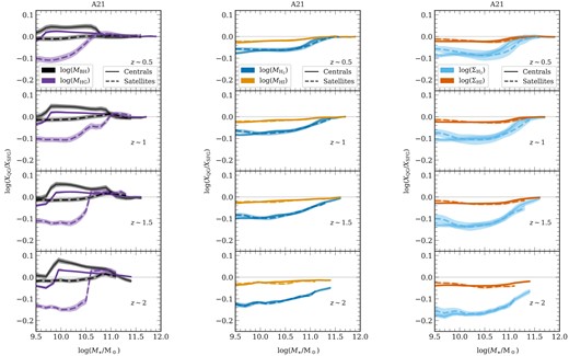
Black hole and hot gas (left), and cold gas distributions (middle and right): The left plot illustrates the logarithmic ratio between BH masses (black lines) and hot gas (HG) masses (purple line), while the plots in the middle and on the right show the distribution of the atomic (|$\rm HI$|) and molecular (|$\rm H_2$|) cold gas. These log-ratios are for the quantities in QGs relative to the SFGs within the A21 model flavour. The middle panel displays mass ratios, while the right panel shows ratios of surface densities of |$\rm HI$| and |$\rm H_2$|. Solid and dashed lines represent central and satellite galaxies, respectively. The scatter within the sample is depicted by the shaded areas.
In A21, the distribution of hot gas and BH mass across galaxy types and masses reveals trends tied to quenching processes. Low-mass quenched central galaxies (|$M_\star \lesssim 10^{9.8}\:{\rm M}_{\odot }$|) have on average less hot gas than their star-forming counterparts, reflecting the impact of ejective stellar feedback. On the other hand, more massive (|$M_\star \gtrsim 10^{9.8}\:{\rm M}_{\odot }$|) quenched centrals exhibit elevated hot gas levels, causing stronger AGN feedback (see equation 2) and, consequently, the cessation of star formation activity. This increased feedback, however, may not entirely represent the astrophysical nature of observed AGNs. Additionally, these quenched centrals tend to have more massive BHs, a direct outcome of the implemented AGN feedback mechanism (see equation 2). Similarly, quenched satellites show significantly less hot gas, highlighting gas stripping in dense environments as the main quenching mechanism. This stripping effect is more pronounced in less massive satellites (|$M_\star \lesssim 10^{10.5}\:{\rm M}_{\odot }$|) and diminishes as satellite mass increases. For the most massive satellites (|$M_\star \gtrsim 10^{10.5}\:{\rm M}_{\odot }$|), AGN feedback is the primary quenching method rather than environmental processes. Additionally, the BH mass ratios show weaker trends but indicate that star-forming satellites, likely due to their abundant hot gas content, experience more substantial BH growth.
The hot gas dynamics in the L-galaxies models illustrate that while stellar feedback and UV background radiation are effective at altering hot gas content in galaxies up to Milky Way mass scales (|$M_\star \sim 10^{10.8}\:{\rm M}_{\odot }$|), they become ineffective in more massive ones. This leads to a hot gas fraction near the cosmic value among these massive systems with minimal scatter, as shown in Fig. 16. Nevertheless, this does not align with various X-ray observations, thus motivating future improvements in the AGN feedback prescription to facilitate the ejection of gas beyond the halo boundary.
5.3 Cold gas distribution
Atomic hydrogen (|$\rm HI$|) and molecular hydrogen (|$\rm H_2$|) are critical for star formation, with SFGs typically harbouring larger fractions of both. In contrast, QGs often show reduced amounts of these gases due to processes like gas depletion, environmental effects, and feedback mechanisms (e.g. Tacconi et al. 2010, 2018; Janowiecki et al. 2020; Guo et al. 2021). Metallicity plays a crucial role in the formation of molecular hydrogen as it provides cooling pathways essential for converting atomic to molecular phases (e.g. Tacconi et al. 2010; Kauffmann et al. 2012). Dust grains, more prevalent in metal-rich environments, facilitate |$\rm H_2$| formation by offering surfaces for hydrogen atoms to combine (e.g. Cazaux & Spaans 2009). Additionally, UV radiation can influence gas phases through photodissociation, impacting the balance between the cold gases.
The middle and right panels of Fig. 17 illustrate the log-ratio between the hydrogen masses (middle) and surface density (right) of QGs relative to those of SFGs in the A21 model. The cold gas surface densities [|$\Sigma _{\rm HI\:or \:H_2}=f_{\rm HI\:or\:H_2}(M_{\rm Cold\:Gas}/2\pi R_{\rm GasDiscRadius}^2$|)] are calculated using the fraction of cold gas mass that is in |$\rm H_2$| or |$\rm HI$| (|$f_{\rm HI\:or\:H_2}$|) and the size of gas disc (|$R_{\rm GasDiscRadius}$|), which is dependent on the halo spin parameter, and the maximum rotational velocity of the subhalo in the simulations (Guo et al. 2011). These distributions are separately analysed for central and satellite galaxies, providing a detailed view of the cold gas dynamics across different galactic environments.
Overall, QGs have a significantly lower fraction of |$\rm H_2$| gas compared to their star-forming counterparts, reflecting our |$\rm H_2$|-dependent star-formation mechanism. This trend typically intensifies towards lower mass galaxies and at higher redshifts. Quenched galaxies also contain slightly less H i gas than star-forming ones, although the difference is not as marked as with |$\rm H_2$| gas. There is no significant distinction between central and satellite galaxies in terms of the cold gas content, primarily due to the absence of cold gas stripping in our model (e.g. Brown et al. 2017). This process will be incorporated into future versions of L-galaxies.
6 DISCUSSION
6.1 Comparison with other work
Recent observations of the high-redshift universe, especially those focusing on massive quenched systems and the detailed characteristics of the UV luminosity function (UVLF) as observed by the JWST (e.g. Bouwens et al. 2023; Carnall et al. 2023), pose significant challenges for galaxy formation simulations. Numerous studies have been struggling to replicate these phenomena accurately. A pivotal challenge is promoting early galaxy quenching, which would significantly impact the high redshift number density of passive galaxies in simulations.
Somerville & Davé (2015) compared the efficacy of three hydrodynamic simulations and five semi-analytical models, including an older L-galaxies model variant (Henriques et al. 2013). This assessment revealed that while the models generally adhered well to established calibration benchmarks, they struggled to produce massive galaxies at higher redshifts. Since then, a number of authors have attempted to solve these problems by changing the treatment of certain physical processes in the simulation.
In a recent study, Lagos et al. (2024) introduced new AGN wind and jet modes based on the properties of the SMBH in the SHARK semi-analytic model (Lagos et al. 2018). Similar to our work, they compared their results with data from Weaver et al. (2023) for the galaxy stellar mass function across different redshifts. They showed that these updates improved the model’s ability to suppress star formation in massive galaxies at later times. Although the number density of quenched galaxies increased by about 0.8 dex at |$z\sim 3$| for |$M_\star \gtrsim 10^{10.5}\:{\rm M}_{\odot }$| systems, the models underpredict the number density of massive galaxies at higher redshifts.
We note that unlike our approach, which solely utilizes the NUVrJ criterion, Lagos et al. (2024) applied both NUVrJ and sSFR cuts to classify galaxies as quenched. They found that alignment with the observational data from Weaver et al. (2023) was more accurate when similar selection criteria (i.e. NUVrJ) were used. Furthermore, the authors introduced a random error of 0.3 dex to account for systematics and uncertainties in the SHARK semi-analytic model’s SMF, an approach we did not adopt in our analysis.
Despite the inclusion of AGN outflows from the cold interstellar medium – a feature not present in the L-galaxies models – SHARK underpredicts |$M_\star \sim 10^{11}\:{\rm M}_{\odot }$| quenched systems by about a factor of |$2-3$| compared to the A21,L-galaxies model at |$z\sim 2$|, signifying that the challenge of the quenching mechanisms is still not solved. Additionally, SHARK overestimates the number density of low-mass quenched systems at lower redshifts in comparison to both the observational data and the L-galaxies models, a common issue in semi-analytical models as is discussed in Harrold et al. (2024).
Finally, we note that Lagos et al. (2024) also updated the SHARK semi-analytic model with a new prescription for galaxy angular momentum, influenced by star formation laws and circular velocity profiles. This update facilitates more accurate predictions of the galaxy mass–size relationships for both bulge and disc components, showing improvements over previous versions and better alignment with observational data at |$z=0$|. Their analysis focused on comparing direct simulation output with observations. Nevertheless, there are significant complexities associated with comparing galaxy sizes with observations. As demonstrated in our comparison of galaxy sizes from L-galaxies with observational data in Section 4.6, the results can substantially change once mock galaxy sizes are determined using the same methodology as applied to observational data, for instance by fitting a single component Sérsic profile (Fig. 11), compared to using raw simulation output. For reference, currently the L-galaxies models follow Mo et al. (1998), assuming that the angular momentum of infalling material aligns with that already present in the galaxy’s disc.
De Lucia et al. (2024) recently evaluated three different versions of the GAEA semi-analytic model (De Lucia & Blaizot 2007), including a version with a new AGN-driven outflow mechanism and updated treatment for low mass satellites, and compared these to findings from Weaver et al. (2023). The GAEA model was calibrated using the stellar mass function up to |$z\sim 3$| and the AGN luminosity function up to |$z\sim 4$|. While the updated GAEA model showed improvements in simulating total and quenched systems up to |$z\sim 4$|, discrepancies remained, albeit smaller than those in earlier versions of their models. It is important to note that they used a sSFR cutoff to classify galaxies as quenched, in contrast to the |$\rm NUVrJ$| criterion used by Weaver et al. (2023) and our paper, potentially introducing systematic biases such as overestimation of the quenched fraction in the simulations. The NUV band captures star formation history over the past billion years, offering a longer term view of the past star formation history than the instantaneous SFR in the model, which only reflects recent activity on the time-scale of a single snapshot. This could lead to an overestimation of quenched galaxies when using sSFR criteria in the model (e.g. Haydon et al. 2020). Including these biases and Gaussian distributed uncertainties in the SMFs, the model predictions fell slightly short of matching the observations at the massive end. The models produced about 2.5 times more |$M_\star \sim 10^{11}\:{\rm M}_{\odot }$| quenched systems at |$z\sim 2$| than the A21L-galaxies model, likely a consequence of the AGN-driven outflows.
In a study by Zoldan et al. (2019), galaxy sizes in an older version of the GAEA model (Xie et al. 2017) were evaluated against observational data from der Wel et al. (2014b). The analysis showed good agreement with the properties of SFGs but less agreement with QGs, yet better than L-galaxies. The model reproduced the steep slope of the galaxy mass–size relation noted by der Wel et al. (2014b). However, the study employed a sSFR cutoff to define quenched systems, differing from der Wel et al. (2014b)’s selection criteria. This likely would have led to an overestimation of the number of quenched systems affecting their median sizes. Moreover, they did not attempt to derive galaxy sizes by fitting a Sérsic profile, an exercise conducted both in der Wel et al. (2014b) and in our study.
Parallel efforts by Yung et al. (2024), showed that the updated Santa Cruz semi-analytic model (Somerville & Primack 1999) underpredicted the UVLF at high and ultra-high redshifts (|$z\gtrsim 8$|) compared to observations. While the L-galaxies models currently lack the capability to probe these ultra-high redshift galaxies due to fewer time snapshots in the MRI and MRII simulations, running L-galaxies on newer simulations such as MillenniumTNG (Barrera et al. 2023; Pakmor et al. 2023) could provide enhanced resolution and better temporal coverage for exploring these early epochs in more detail.
6.2 Interpretation of the results
In light of the interactions between hot gas, black holes, and cold gas across different galactic environments, detailed in Section 5, our findings suggest several avenues for refining future astrophysical prescriptions in the L-galaxies framework.
The relationship between baryon or gas fraction and halo mass (|$f_{\rm b \:or \: gas} -M_{200}$|) is now becoming much better constrained at low redshifts. However, a discrepancy exists with current observational data suggesting that more baryons need to be expelled in galaxy groups. This inconsistency arises because the L-galaxies model predicts a redshift-independent relationship for these fractions, owing to the scaling of SN and AGN feedback efficiencies with halo-mass rather than internal galactic properties (Fig. 16). Future observations (e.g. Ade et al. 2019; Kraft et al. 2022; Zhang et al. 2024) may provide further light on this matter, potentially driving refinements in feedback mechanisms within the L-galaxies framework.
Our investigation of the differences between hot gas, black holes, and the masses of cold gas in atomic and molecular form in SFGs and QGs yields the most insightful results (Fig. 17). The findings highlight strong differences primarily in low-mass satellite galaxies, where differences in the hot gas distribution is more pronounced. In contrast, central galaxies, which are the highest mass galaxies at all redshifts, exhibit almost no differences in these parameters. However, a notable distinction is observed in quenched galaxies at high redshifts, where the molecular gas content of both centrals and satellites has been strongly depleted, indicating the important role of the internal gas reservoir in regulating the star-forming state of these high-z galaxies.
These findings may support the AGN feedback model enhancements implemented into the SHARK semi-analytical model. Combining these enhancements with the Ayromlou et al. (2019) gas stripping prescriptions could alleviate some of the discrepancies in the SHARK model, particularly concerning the fitting of low-mass quenched galaxies. However, if the inflow of gas into the molecular reservoir and its consumption rate into stars has not been accurately parametrized at very high redshift, changes to the AGN feedback recipes may be spurious.
Studies on galaxy growth mechanisms, such as those by Genel et al. (2018) and Ferrero et al. (2021), corroborate that quenched galaxies expand predominantly through dry mergers and tidal interactions following their quenching episodes. Furthermore, studies by Taylor & Kobayashi (2016), Trayford & Schaye (2019), and D’Onofrio & Chiosi (2023) agree that galaxy merging is crucial in galaxy size evolution, with AGN feedback playing a substantial role in reducing central gas densities and influencing the compactness of galaxies’ central regions. These studies, on the other hand, highlight the significant role of galaxy morphology and mass in these processes, and suggest the necessity of incorporating more explicit mechanisms for modelling the impacts of merging and feedback on galaxy sizes and structures within L-galaxies models.
In contrast, the L-galaxies models currently lack advanced prescriptions for modelling the detailed impacts of merging on galaxy sizes and structures, and AGN outflows. The L-galaxies models currently utilize the prescription from Guo et al. (2011), which relies on energy conservation and the virial theorem to compute the changes in galaxy sizes during mergers. In addition, the bulge component of the galaxies follows a Jaffe (1983) distribution. Overall, addressing the complexities in the galaxy mass–size relations remains challenging and requires careful implementation of various physical processes.
Finally, observational studies of MgII absorbers in the vicinity of radio-loud AGN provide evidence that AGN influence the gas around galaxies even outside their dark matter haloes (Kauffmann 2018). This redistribution of the gas within and beyond the halo boundary, out to the closure radius, due to AGN feedback adds substantial complexities to the physics of galaxy evolution (Ayromlou, Nelson & Pillepich 2023). Further exploration of these mechanisms and their long-term effects on galaxy evolution is essential and reserved for future studies.
In forthcoming work, we plan to explore a variety of physical parameter changes that could help us to match the high redshift data with better accuracy. MCMC and more modern machine learning parameter optimization techniques are expected to be very useful tools in this endeavour.
7 SUMMARY AND CONCLUSION
The study of galaxy evolution across cosmic epochs is essential for assessing cosmological galaxy formation models against observational data, thereby guiding future model refinements. In this study, we present a rigorous evaluation of three calibrated versions of the L-galaxies cosmological galaxy evolution semi-analytical model; namely A21, H20, and H15, across a broad range of masses (|$10^7\: {\rm M}_{\odot }\lesssim M_\star \lesssim 10^{12}\:{\rm M}_{\odot }$|) and redshifts (|$0\le z \lesssim 10$|). A key novel aspect of this work is the incorporation of high-redshift observations and an in-depth analysis of galaxy size and stellar mass surface density evolution. The analysis systematically compares simulated galaxy properties with observational data to assess the fidelity of these models in reproducing key aspects of galaxy evolution, including stellar mass functions, cosmic star formation rate densities, galaxy size–mass relations, and the evolution of core |$(R\lt 1\, {\rm {kpc}})$| and effective |$(R\lt R_{\rm {e}})$| stellar mass surface densities, both for star-forming and quenched galaxies. Here are our key findings:
Total SMF: The L-galaxies flavours align well with observations up to |$z\sim 7.5$| for all mass ranges with small deviations (Fig. 4).
CSFRD: While the simulations capture the general trend up to |$z\sim 10$|, they exhibit a slightly suppressed SFR at |$z\sim 2$| by a factor of 1.2–1.5 (Fig. 5).
SFG SMF: The three model flavours align well with the observations at low-to-intermediate redshifts |$(z \lesssim 2)$|, however, at higher redshifts, small discrepancies emerge for |$M_\star \sim 10^{10}\:{\rm M}_{\odot }$| galaxies (Fig. 6).
QG SMF: The A21 model flavour shows a closer agreement and predicts a more accurate match to the observed SMF and the number density of QGs at lower redshifts. However, despite A21’s qualitative agreement with observations in the evolution of the SMF of QGs, all L-galaxies flavours underpredict the abundance of QGs at |$z \gtrsim 1.5-2$| for |$M_\star \gtrsim 10^{10.5}\:{\rm M}_{\odot }$| galaxies. This discrepancy grows from a factor of 1.5 at |$z \sim 2$| to a factor of 60 by |$z \sim 3$| for the |$M_\star \sim 10^{11}\:{\rm M}_{\odot }$| quenched systems (Figs 7 and 8).
QG number density|$-z$|: The L-galaxies flavours exhibit a transition in dominance from satellites to centrals in the number density of QGs around |$M_\star \sim 10^{10.2-10.3}\:{\rm M}_{\odot }$|, highlighting a shift in the primary quenching mechanisms at these mass scales (Fig. 8). Below this threshold, environmental effects predominantly drive quenching, whereas, above it, AGN feedback becomes the main quenching mechanism.
|${\rm SFR}-M_\star$|: All three model flavours reproduce the star-forming main sequence relationship effectively up to |$z\sim 6$|. However, they often miss the flattening of this relation for the most massive (|$M_\star \sim 10^{11}\:{\rm M}_{\odot }$|) galaxies at |$z\gtrsim 5$|, also showing a suppressed SFR at |$z\sim 2$| (Figs 9 and 10).
|$R_{\rm e}-M_\star$|: While massive SFGs and QGs show consistency with the observations up to |$z\sim 3$|, SFGs and QGs with mass |$M_\star \lesssim 10^{10.5}\:{\rm M}_{\odot }$| and |$M_\star \lesssim 10^{11.2}\:{\rm M}_{\odot }$|, respectively, tend to have larger sizes by a factor of up to 15 than observed, with the greatest deviations occurring in quenched systems (Figs 11 and 12).
|$\Sigma -M_\star$|: For the SFGs the core (|$R\lt 1\:{\rm kpc}$|) and effective (|$R\lt R_{\rm e}$|) stellar mass surface densities are generally in alignment up to |$z\sim 3$| for all masses with small deviations. At |$z \sim 0.5$|, QGs with |$M_\star \sim 10^{10}\:{\rm M}_{\odot }$| are significantly less compact than expected, undercompact by a factor of |$\sim 4$| in the |$\Sigma _{1\:{\rm kpc}}-M_\star$| plane and by |$\sim 80$| in the |$\Sigma _{R_{\rm e}}-M_\star$| plane (Figs 13, 14, and 15).
A central focus of this work is the discrepancies observed from |$z\gtrsim 2$|. Without high-redshift comparisons, it is not possible to determine the direction for future improvements in the L-galaxies model, emphasizing the importance of high-z data in shaping our understanding of galaxy formation. Notably, our results highlight that the primary discrepancy arises not from advanced gas stripping prescription in low-mass galaxies, but rather from the galaxy quenching mechanisms, likely the AGN feedback and galaxy merging mechanism, in more massive galaxies. This issue becomes increasingly apparent beyond |$z \gtrsim 1.5$|, suggesting that future iterations of L-galaxies must revisit galaxy quenching implementations.
In conclusion, our investigation indicates that while significant strides have been made in physically simulating realistic galaxy populations, critical discrepancies persist, particularly at high redshifts and in representing the number density, size, and surface density distributions of quenched galaxies. Our analysis has identified several avenues for potential improvements in the L-galaxies framework. These include revising galaxy quenching mechanisms – for example AGN feedback – as well as implementing a more physical treatment for galaxy mergers, which are crucial for accurately modelling the size and surface density distribution of quenched systems. To navigate these issues and effectively generate new models and prescriptions, we aim to develop tools using machine learning, that can more efficiently probe the parameter space. To mitigate calibration biases, we also plan to recalibrate the model using an MCMC approach with the latest high-redshift observational data, which were not available during the last calibration of the L-galaxies model. Incorporating data from new observational facilities like JWST and utilizing the results of the most recent hydrodynamical simulation projects such as MillenniumTNG (Pakmor et al. 2023) and FLAMINGO (Schaye et al. 2023) are expected to provide fresh insights that can guide the design of future versions of the L-galaxies model, further enhancing the reliability and accuracy of its predictions.
ACKNOWLEDGEMENTS
The analysis herein was carried out on the compute cluster of the Max Planck Institute for Astrophysics (MPA) and systems at the Max Planck Computing and Data Facility (MPCDF). AV wants to thank Bo Peng, Silvia Bonoli, Rachel Somerville, Greg Bryan, Rob Yates, Stephanie Tonnesen, and Anshuman Acharya for the useful discussions and assistance. MA extends gratitude to Moein Mosleh for the insightful conversations. MA also acknowledge funding from the Deutsche Forschungsgemeinschaft (DFG) through an Emmy Noether Research Group (grant number NE 2441/1-1). This work has made use of: Astropy (Astropy Collaboration 2018), TOPCAT (Taylor 2005), Scipy (Virtanen et al. 2020), Seaborn/Matplotlib (Hunter 2007; Waskom 2021), and the National Aeronautics and Space Administration (NASA) Astrophysics Data System (ADS).
DATA AVAILABILITY
The full outputs of the three L-galaxies flavours for all the Millennium-I and Millennium-II snapshots are publicly available at http://lgalaxiespublicrelease.github.io/.
Footnotes
The models can be found at https://lgalaxiespublicrelease.github.io/, which also includes complete documentation for all three model flavours.
|$t_{{\rm H}(z=0)}$| is the Hubble time at |$z=0$|.
defined as |$\Delta I_{\text{residual}}=\Sigma _{i=0}^{r_i} (I(r)_{\rm {\small l-galaxies}{}}/I(r)_{\rm{1D S'{e}rsic}}-1)^2/{\rm dof}$|, where |$\Sigma$| sums over the squared deviations of surface brightness (I) at different galactic radius (r) for each galaxy and |$\rm dof$| is the degree of freedom.
The radius encompassing 200 times the critical density of the universe.
Mass within |$R_{200}$|.
REFERENCES
APPENDIX A: RESULTS FROM H20 AND H15
The results of classifying SFGs and QGs in the H15 flavour, using the |$\rm NUVrJ$| colour–colour selection criterion (refer to equation 4), are shown in Fig. A1. Notably, the H15 flavour exhibits red-ward scatter in the |$\rm NUVrJ$| plot, which could be attributed to its older star formation prescription which maintains a fixed ratio of atomic to molecular hydrogen. This trend towards redder colours is independent of the dust models, which are consistent across all L-galaxies flavours (Devriendt et al. 1999; Charlot & Fall 2000). Both the H20 and H15 flavours exhibit a deficit of quenched systems starting at |$z \gtrsim 2-3$|, similar to the trends observed in the A21 flavour.

Fig. A2 illustrates the |${\rm sSFR}-M_\star$| plot for the chosen quenched systems modelled by the H15 flavours, showing trends and distributions similar with those observed in A21. Notably, there is a minor degree of contamination from galaxies with slightly higher sSFRs than the established cutoff threshold (|$f_{\text{QG}}$|), as highlighted in Section 4.1. These ‘contaminating’ galaxies are predominantly massive satellite galaxies, with the fraction of such contaminants decreasing with increasing redshift.

Fig. A3 shows the total SMF (top panel), the SFG SMF (middle panel), and QG SMF (bottom panel) for the H15 with the dashed line representing the observational fits from Weaver et al. (2023) along with its one-sigma errors. Similarly, Fig. A4 shows the QG SMF for the H20 model flavour. Overall the conclusions are similar to the ones mentioned for A21 with small deviations as mentioned in Section 4.2.1, 4.3, and 4.4.
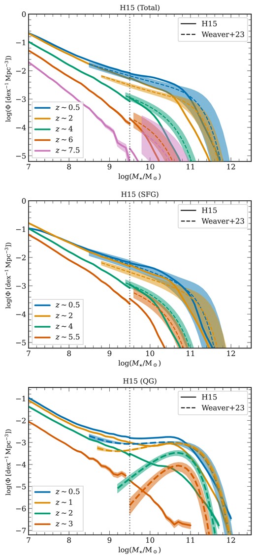
Stellar mass functions: These plots display the total SMF (top), the star-forming galaxy SMF (middle), and the quenched galaxy SMF (bottom) for the H15 model flavour. In these plots, the solid line shows the evolution of the stellar mass functions from the simulations across five redshifts, and the dashed line is from the observational findings of Weaver et al. (2023). The plot is similar to Figs 4, 6, and 7.

Fig. A5 shows the main sequence of star-forming galaxies for H15 with observational fits from Popesso et al. (2023) and Speagle et al. (2014) in red and yellow solid lines.

APPENDIX B: CONVERGENCE OF MRI AND MRII
As is extensively discussed in Boylan-Kolchin et al. (2009), the halo mass function and the subhalo mass function exhibit excellent convergence between MRI and MRII. For completeness, these two relations are reproduced in Fig. B1 for five representative ranges of redshift bins. The results from MRI are shown by the solid lines, while the dashed lines represent the smaller box of MRII.
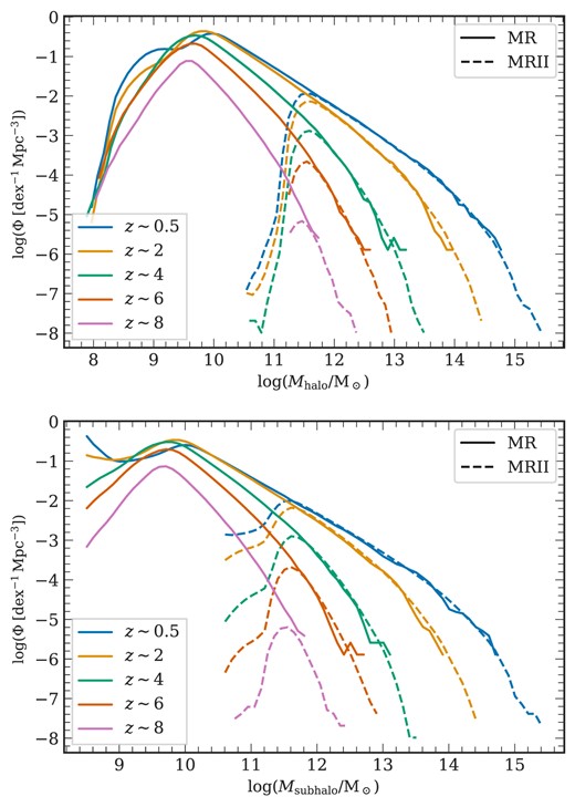
These plots show the halo mass function (left) and the sub-halo mass function (right). The colour coding represents the redshift bin for which the mass function is plotted. The solid and dashed lines represent the MRI and MRII simulations.
Any observed deviation in the galaxy scaling relation plots discussed in this study between the MRI and MRII boxes arises from the divergence of the physical models at the resolution limit boundary. The choice of the transition region between MRI and MRII and among different scaling relations could result in better or more unsatisfactory convergence of these relations. Using a different transition mass for each L-galaxies flavour does not change any of our results or conclusions significantly (e.g. refer to Fig. 7).
APPENDIX C: SÉRSIC PROFILE FITTING
The two L-galaxies flavours with radial rings (A21 and H20) use a curve of growth approach, iteratively finding the radius that contains half of the total flux of the galaxy, to calculate the half-light radii (|$R_{\rm e}$|). However, the observational works of der Wel et al. (2014a) and Mowla et al. (2019), which we use for comparison, employ the Sérsic (1963) profile to derive the effective radius. Thus, to facilitate a meaningful comparison between observations and simulation data, we derive the |$R_{\rm e}$| from a single-component 1D Sérsic profile fit. The Sérsic profile is expressed as:
where |$I_0$| is the intensity or brightness at the centre of the galaxy (|$r=0$|), |$R_{\rm e}$| is the half-light radius, n is the Sérsic index, determining the shape of the profile, and |$b_n$| is a constant related to n.
Assuming the mass-to-light ratio to be unity, we calculate the cumulative light contribution from the disc and bulge regions. Furthermore, the surface brightness profile is determined by normalising the cumulative light contribution by the area of the respective ring. Using this data, we fit a 1D Sérsic profile, as shown in Fig. C1. The blue data points represent the data from the L-Galaxies model. These data points exhibit a complex shape, and fitting a single power law may not capture this complexity well. Different galaxies have complex surface brightness profiles; for example, they could have a flat inner bulge or a flared outer disc. The blue dotted line in Fig. C1 represents the Sérsic fit (SF) for these data points from simulated galaxies, resulting in |$R_{\text{e, SF}}$| indicated by the blue dashed vertical line, while the black dashed vertical line provides |$R_{\text{e, CoG}}$| derived by the curve of growth approach used by the L-Galaxies model.
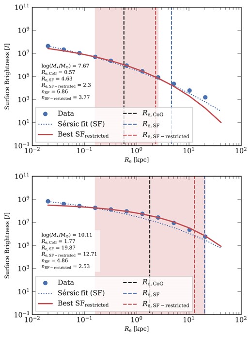
These two plots illustrate the surface brightness profile (I) of two randomly selected galaxies in the A21 model flavour. The one on the left represents the surface brightness profile of a |$M_\star =10^{7.67}\:{\rm M}_{\odot }$| galaxy from MRII, while the plot on the right shows the surface brightness profile of a |$M_\star =10^{10.11}\:{\rm M}_{\odot }$| galaxy from MRI. In both plots, the blue dots represent the data points from simulated galaxies, and the blue dotted line is the 1D Sérsic fit (SF) for these data points, with the |$R_{\rm e, SF}$| indicated by the vertical blue dashed line. The red-shaded region in each plot represents a restricted region used for fitting the 1D Sérsic profile. The restricted fit is shown as the solid red line, with the |$R_{\rm e, SF-restricted}$| denoted by the vertical red dashed line. The |$R_{\rm e, CoG}$| derived by the curve of growth approach in L-galaxies is given by the black dashed vertical line.
Upon inspection, we realized that fitting a Sérsic profile in a restricted galactocentric radial range simplifies the complex profile, making it resemble a single power-law profile. This is achieved by excluding the bulge region and the faint end of the outer disc of the galaxy, by incorporating a limiting surface brightness cut, |${ I_{\rm limit}} = 26.6 \,\, [\rm mag\,\, arcsec^{-1}]$| (Papovich et al. 2012). Thus, we fit the surface brightness profile within |$0.2 \:{\rm kpc}\lt R\lt R_{\rm I,limit}$|, where |$R_{\rm I,limit}$| is the galactocentric radius at which the galaxy reaches the surface brightness limit. This is highlighted as the red-shaded region, and the fit is represented by the solid red line. The red dashed vertical line denotes the effective radius (|$R_{\text{e, SF-restricted}}$|) for this fit. It is ensured that the red-shaded region includes at least three data points for fitting the Sérsic profile. The plots also display the mass of the galaxy and the other fitting parameters.
