


ABSTRACT
The absence of neutral gas in Local Group dwarf spheroidal galaxies is a well-known fact. However, the physical mechanism that led to the removal or consumption of their gas remains an unsolved puzzle. It is possible that galactic winds triggered by supernovae or external physical processes such as ram pressure or tidal stripping could have played a significant role in removing a considerable portion of gas from these galaxies. This study utilizes a non-cosmological 3D hydrodynamic simulation code to explore the impact of feedback from Types Ia and II supernovae on the dynamics of the gas of a typical dwarf spheroidal galaxy. The simulation code considers a fixed and cored dark matter potential and a ratio of baryonic to dark matter based on cosmic background radiation, and it takes into account the effects of both Type II and Type Ia supernova feedback. The gas distribution inside the tidal radius of the galaxy is allowed to evolve over 1 billion years considering different prescriptions for the spatial and temporal distribution of the supernovae. Our results suggest that Type Ia supernovae are more effective in expelling the gas out of the galaxy whereas Type II supernovae remove the gas from the central regions of the system. Whereas the spatial distribution of supernovae is more influential on gas loss than their temporal distribution, both factors should be considered in stellar feedback studies. Moreover, both types of supernovae, with their distinct time-scales, should be incorporated into these investigations.
1 INTRODUCTION
When the first classical dwarf spheroidal galaxies (dSphs) were detected (Shapley 1938, Wilson 1955), they were thought to be simple systems, very similar to globular clusters, without complex structures, with a single stellar population, and uniform chemical properties. As more detailed observations emerged, the scenario changed drastically. It is now known that these galaxies are characterized by different stellar populations, chemical enrichment not yet fully explained, complex star formation histories, and exhibit a large amount of dark matter (DM; Mateo 1998; Tolstoy, Hill & Tosi 2009; McConnachie 2012). Completing this scenario, all analysed dSphs share a common feature: the total absence of detectable neutral gas (Grcevich & Putman M. 2009; Spekkens et al. 2014).
How the gas is removed from the galaxy or is consumed internally remains a critical point without a consensus, even though there are several observational constraints that can shed some light into this matter. Chemical properties observed in local dSphs, for instance, suggest that a large fraction of the galactic gas was lost during the evolution of the galaxy either as a consequence of internal physical processes or due to external mechanisms. Gas loss driven by galactic winds triggered by supernovae (SNe) coupled to a low star formation efficiency (down to 100 times lower than in the solar vicinity) is required in some chemical evolution models to fit particular chemical abundance ratios, the stellar metallicity distribution, and the age–metallicity relation observed in local dSphs (Lanfranchi & Matteucci 2003; Lanfranchi & Matteucci 2004; Lanfranchi & Matteucci 2007; Salvadori, Ferrara & Schneider 2008; Kirby E., Martin & Finlator 2011). These models not only reproduce the present-day chemical properties of local dSphs but also account for the very low fraction of remaining gas in these systems. In other works, however, external mechanisms such as tidal stripping or ram-pressure are invoked to explain the lack of gas in dSphs after the observed chemical properties are settled (Marcolini et al. 2006, 2008; Revaz et al. 2009; Revaz & Jablonka 2012). In either scenarios, the details of the gas loss (e.g. galactic wind efficiency and gas loss rate) are normally adjusted ad hoc to fit the observations.
Following a different approach, the flux of gas inside the galaxy and the amount of gas that is either blown out or blown away can be calculated consistently by means of hydrodynamic simulations. Early simulations suggested that galactic winds triggered by SNe are not able alone to remove all the gas from the medium of dwarf galaxies, unless in specific conditions. This would be possible only for systems with |$\sim 10^{5-6}$| M|$_{\odot }$| (Mac Low & Ferrara 1999; Fragile et al. 2003; Sawala et al. 2010; Stringer et al. 2012). However, these conclusions depend on the star formation history and number of SNe adopted (Mori, Ferrara & and Madau 2002; Ruiz et al. 2013): an intense stellar formation can give rise to an efficient galactic wind, whereas a low SNe rate is not sufficient for the removal of the interstellar gas from the galaxy. Wada & Venkatesan (2003) analysed the effects of SNe in the medium of primordial galaxies by means of chemodynamic simulations and concluded that the chemical composition and the final structure of the medium depend of the number of SNe considered. For a higher number of SNe (1000), the gas content of the galaxy is almost totally blown away, but if this number is lower (100), gas collapses forming a clumpy disc. In almost all these studies, the SNe occur at the same time in the central region of the galaxy, however, there must be differences in the efficiency of the stellar feedback according to the spatial and temporal distribution of the SNe (McQuinn, van Zee & Skillman 2019). More recently, adopting spatial and temporal distributions of the SNe, Caproni et al. (2015, 2017) performed 3D hydrodynamic simulations adjusted to the dSph Ursa Minor and concluded that the SNe, with a rate constrained by observations, can inject enough energy into the interstellar medium (ISM) to expel |$\sim 60{{\ \rm per\ cent}}$| of the gas of the system inside the tidal radius and up to |$\sim 85{{\ \rm per\ cent}}$| of the central region (300 pc) in a 3 Gyr time-scale. In these works, however, there was no distinction between Type II and Type Ia SNe.
In a more general context, understanding the details of stellar feedback (and also active galactic nucleus, AGN, feedback) in galaxies is of central interest in cosmologic and galactic studies, being a critical component of the evolution of galaxies (Ferrara & Tolstoy 2000; Mashchenko, Couchman & Wadsley 2006; Mashchenko et al. 2008; Ceverino & Klypin 2009; Hopkins & Kereš 2014; Muratov et al. 2015; Somerville & Davé 2015; Naab & Ostriker 2017, and references therein). Silk (2017) proposed that AGN feedback in dwarf galaxies could provide explanations for several cosmological issues, such as abundance, core-cusp, too-big-to-fail, ultra-faint, and baryon-fraction ones. On the other side of the feedback spectrum, the stellar feedback can account for the low star formation rates in small galaxies, reconciling the predictions of cosmological simulations with observations (Ceverino & Klypin 2009; Stinson et a. 2012, and many others).
In this work, we investigate the interaction between the energy released by Types II and Ia SNe with the ISM of a dSph by taking properly into account the stellar lifetimes, adopting different prescriptions for their spatial distribution, and SNe rates derived from chemical evolution models that reproduce the main observational chemical properties of the Ursa Minor galaxy (adopted as a template dSph). In such conditions, we also analyse the hydrodynamic evolution of the galactic gas. In Section 2, the numerical code is described, the results are then explained in Section 3 followed by a discussion and the conclusions in Section 4.
2 NUMERICAL SET-UP AND INITIAL CONDITIONS
The different roles played by different types of SNe (Types II and Ia) in the internal dynamics and in the gas removal of a typical isolated dSph are investigated by means of non-cosmological, 3D hydrodynamic simulations of its gas (in this type of simulations, stars are not considered). The galactic gas distribution is evolved for 1 Gyr taking into account both SNe II and SNe Ia, assuming an initial baryonic-to-dark-matter ratio derived from the cosmic microwave background radiation and a cored and static DM gravitational potential. The initial set-up of the simulation is exactly the same one adopted for Ursa Minor dSph (used as a template for a classical dSph), described in details in Caproni et al. (2015, 2017) and Lanfranchi et al. (2021). The ISM is initially in hydrostatic equilibrium with the DM potential (as suggested by Mac Low & Ferrara 1999). The total mass of the DM halo (M|$_\mathrm{ h}$|) is estimated from the core radius r|$_0$| = 300 pc, the initial sound speed in the medium c|$_\text{s}0$| = 8.5 km s|$^{-1}$|, and the circular velocity in Ursa Minor v|$_\text{c}$| = 21.1 km s|$^{-1}$| (Irwin & Hatzidimitriou 1995, Strigari et al. 2007), yielding a value of M|$_\text{h}$| = 1.51 |$\times$||$10^9$| M|$_{\odot }$|. The estimated initial total gas mass is M|$_\text{g}0$| = 2.94 |$\times$||$10^8$| M|$_{\odot }$| and the initial central density is |$\rho _0$| = 3.11 |$\times$||$10^{-22}$| g cm|$^{-3}$|. The dynamics of the galactic gas is simulated for 1 Gyr, using a computational box almost three times as large as the tidal radius (r|$_\text{t}$| = 950 pc), divided in 290|$^3$| cells, with different sizes in different regions. In the most central region of the galaxy, within a cube from −100 to 100 pc, there are 80|$^3$| cells, resulting in a resolution of 2.5 pc per cell side. From 100 to 300 pc (and −100 to −300 pc) the cube is divided in 40 cells per side, each cell with a side of 5.0 pc, and from 300 to 600 pc (and −300 to −600 pc) there are 30 cells per side (resolution of 10 pc per cell). Reaching the tidal radius, from 600 pc to 1 kpc (and −600 pc to −1 kpc) each of the 20 cells has a dimension of 20 pc per side. This resolution allows the code to resolve the shell formation radius of an SN remnant (e.g. Kim & Ostriker 2015; Sarbadhicary et al. 2023) in almost the whole computational domain. All simulations in this work were performed in the Brazilian supercomputer SDumont.1
2.1 The hydrodynamic code
Following previous works of the group (Caproni et al. 2015, 2017; Lanfranchi et al. 2021), 3D hydrodynamic simulations of a typical dSph were performed with the computational code pluto2 (Mignone et al. 2007), adopting the same prescriptions as previously.pluto is an adaptive mesh code that adopts an Eulerian grid-based method, following the evolution of the galactic gas only (there are no stars in the simulations). The numerical code solves the classical hydrodynamic differential equations in each cell:
where |$\rho$| represents the mass density, the fluid velocity in Cartesian coordinates is given by |${\bf {v}}=(v_\mathrm{x}, v_\mathrm{y}, v_\mathrm{z})^T$|, P is the thermal pressure, and |$\mathbf {I}$| and E are, respectively, the identity tensor of rank 3 and the total energy density.
where |$\rho \epsilon$| is the internal density energy. The ideal equation of state |$P = (\Gamma -1)\rho \epsilon$| was adopted in this work, where |$\Gamma$| is the adiabatic index of the plasma, assumed as 5/3. This choice implies in a sound speed of the plasma, |$c_\mathrm{s}$|, defined as |$c_\mathrm{s}=\sqrt{\Gamma P/\rho }$|.
The quantity |$F_\mathrm{c}$| in equation (3) is the cooling function
where n is the number density of the gas and |$\Lambda (T)$| is obtained from the interpolation of the precomputed tables provided by Wiersma, Schaye & Smith (2009). Following Caproni et al. (2015), to compute the values of |$\Lambda (T)$|, we adopted |$n=0.1$| cm|$^{-3}$|, roughly the initial mean number density inside the simulated box domain, and [Fe/H] |$\sim -2.13$|, the median metallicity of Ursa Minor (Kirby et al. 2011).
The initial distribution of the gas density (Fig. 1) and gas density and temperature profiles (Fig. 2, left column) were fully determined imposing hydrostatic equilibrium between an initial isothermal gas with sound speed, |$c_\mathrm{s_0}$|, and a cored, static DM gravitational potential, |$\Phi _\mathrm{h}$| (Binney & Tremaine 2008; Mac Low & Ferrara 1999):
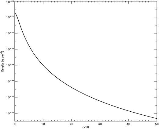
Initial gas density as a function of distance, expressed in terms of the characteristic radius, |$r_0$|.
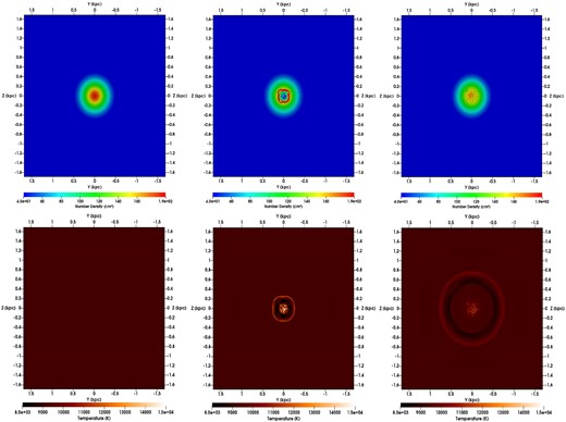
Cut in the |$x = 0$| plane for the gas density (top) and gas temperature (bottom) of the gas at t = 0 Myr (left), 3 Myr (centre), and 12 Myr (right) for the simulation SNcenterT0.
generated by an isothermal, spherically symmetric DM mass density profile with a characteristic radius, |$r_0$|, equals to 300 pc. In equation (6), |$\xi = r/r_0$|, r is the radial distance, and |$v_\mathrm{c_\infty }$| is the maximum circular velocity due to the DM gravitational potential, assumed to be equal to 21.1 km s|$^{-1}$| (in agreement with Strigari et al. 2007).
2.2 Energy injection
Because the simulations adopted in this work do not consider stars and therefore do not support star formation, stellar feedback is emulated by injecting the energy released by SNe, considering in details both types of SNe (Type II and Type Ia). The choice of considering only the feedback from SNe comes from the much higher amount of energy released by these explosions (an order of 10|$^{51}$| erg each SN) compared to stellar winds (|$\sim 10^{35}$| erg) (Bradamante, Matteucci & D’Ercole 1998; Romano et al 2019) and is justified by the results of Romano et al (2019). These authors examined the role played by stellar feedback in the Bo’otes I ultra-faint dwarf galaxy by means of high-resolution 3D hydrodynamic simulations, considering the energy and mass injected in the ISM by OB associations and SNe. The energy of pre-SN phase is considered from 0 to 3 Myr, but their effect is negligible and the medium is hardly disturbed. One can notice modifications in the ISM only after the onset of the SNe (3–30 Myr) in these associations, even though they are not sufficient to remove gas from the galaxy.
Contrary to previous works (Mac Low & Ferrara 1999; Fragile et al. 2003; Romano et al 2019), the SNe in this work are distributed over space and over time and during a much longer time-scale (up to 1 Gyr). The SNe distribution over time is taken from the results of chemical evolution models that reproduce several observed chemical properties of Ursa Minor (Lanfranchi & Matteucci 2004, 2007). The observed abundance ratios (especially [|$\alpha$|/Fe]), stellar metallicity distribution, and gas mass imply in a low star formation rate and, consequently, a low SNe rate, since the number of SNe is directly linked to the number of stars formed. On the other hand, the stellar lifetimes, taken properly into account in the chemical evolution models, and the prescriptions adopted for SNe II and SNe Ia define their distribution over time. Single massive stars, with M|$\ge$| 8 M|$_{\odot }$|, end their evolution as a SN II in a time-scale shorter than |$\sim$|30 Myr (lifetime of a 8 M|$_{\odot }$| star) whereas binary systems of stars of intermediate mass (M|$\sim$| 3–8 M|$_{\odot }$|) give rise to SNe Ia when the most massive star of the system, after evolving and becoming a white dwarf, accretes mass from the less massive one in the red giant or white dwarf phase. The time-scale for the occurrence of the SNe Ia is controlled, consequently, by the evolution of the less massive star of the binary system, that could take more than 1 Gyr to become an SN (Matteucci & Greggio 1986). Given that, different types of SNe give rise to different SNe rates with a maximum value occurring at different epochs: for SNe II, the rate and its maximum follow strictly the star formation rate, but the time-scale for the maximum in the SN Ia rate is a strong function of the adopted stellar lifetimes, initial mass function, and star formation rate (Matteucci & Recchi 2001). In the case of Ursa Minor, there is a distinct maximum in the SNe II rate at a galactic age of |$\sim$|400 Myr whereas for SNe Ia there is no peak in the distribution, but a plateau from 0.8 to 1 Gyr.
All these facts considered lead to individual prescriptions for the injection of energy by Types II and Ia SNe, differing from the approach of the other works of the group (Caproni et al. 2015, 2017; Lanfranchi et al. 2021). In both cases, the SN rates from the chemical evolution models are followed and the energy of a single SN (10|$^{51}$| erg) is injected in the medium (within a spherical region with a diameter of two cell lengths) every time t|$_\text{snia}$| or t|$_\text{snii}$| is achieved. The location (computational cells) where the energy is injected in each case, however, follows different prescriptions. For SNe II, the choice of the site for the injection of energy depends on the gas density of each computational cell (as it was adopted for all SNe in Caproni et al. (2015, section 2.2.5), since the time-scale for the occurrence of this type of SN is short (up tp |$\sim$|30 Myr) and it must occur very close to dense region where the star was formed. In a time-step t|$_\text{snii}$|, the cell with the highest density is chosen; if there is more than one cell with the same highest density, one of them is randomly chosen. SNe Ia, however, take a much longer time to occur (up to |$\sim$|1 Gyr) and the stellar system that originates the explosion could be far away from the dense region where it was formed or the gas of the dense molecular cloud could be all swept up. Given that, the cell where the energy of SNe Ia is injected can be located anywhere in the galaxy: the choice is completely random. In all cases studied, no more than 50 000 SNe were considered for the sake of computational time required to run the simulations.
3 RESULTS
The dynamics of the ISM in a dSph was analysed using a 3D hydrodynamic code calibrated to the Ursa Minor galaxy, to understand the distinct roles of SNe II and Ia. (Caproni et al. 2015, 2017; Lanfranchi et al. 2021). Different scenarios were adopted for the injection of energy, with SNe II and SNe Ia occurring in a specific position and time, distributed over limited time and space, and distributed randomly in space. The simulations start at t = 0 yr, with the interstellar gas in hydrostatic equilibrium with the gravitational potential of the galaxy. The initial gas density and the pressure profiles (first and second columns, first line in Fig. 2) of the gas are almost homogeneous (varying only with the radius) with a spherical distribution at the beginning of the simulation, whereas the temperature is constant all over the galaxy (first column, second line in Fig. 2), at around 5.2 |$\times$| 10|$^3$| K. A major fraction of the gas lies within a spherical region with a radius of |$\sim$|300 pc, with a central gas density of 3.11 |$\times$| 10|$^{-22}$| g cm|$^{-3}$|, decreasing to |$\sim$|5.15 |$\times$| 10|$^{-28}$| g cm|$^{-3}$| outside the galactic virial radius. From this point, the energy of the SNe is injected into the galaxy according to various scenarios (Table 1).
Specifications of the SN scenarios in different simulations.
| Simulation | SNe II | Site SNe II | Time SNe II | SNe Ia | Site SNe Ia | Time SNe Ia |
|---|---|---|---|---|---|---|
| SNcenterT0 | 10 000 | x=y=z = 0 | 0 Gyr | – | – | – |
| SNIILM | 10 000 | Density | LM07 | – | – | – |
| SNIaLM | – | – | – | 10 000 | Random | LM07 |
| SNIILMr | 10 000 | Random | LM07 | – | – | – |
| SNIaLMd | – | – | – | 10 000 | Density | LM07 |
| SN4505LM | 45 000 | Density | LM07 | 5000 | Random | LM07 |
| SN3020LM | 30 000 | Density | LM07 | 20 000 | Random | LM07 |
3.1 10 000 SNe in the central point at t = 0 yr
Initially, a simple scenario, similar to previous works (Mac Low & Ferrara 1999; Ferrara & Tolstoy 2000; Wada & Venkatesan 2003, and many others) is adopted in the simulation SNcenterT0. The energy of 10 000 SNe (there is no difference between Types II and Ia) is injected in the central cell of the computational box at the very beginning of the simulation. Soon after the energy is inserted in the ISM (at 3 Myr), a powerful, symmetrical shockwave originates at the galaxy’s core and expands outwards. It propagates fast (v|$\sim$|10–15 km s|$^{-1}$| at t = 3 Myr) towards outer regions, creating thin layers and filaments of high pressure and temperature (|$\sim$|2.2 |$\times$| 10|$^4$| K) (Fig. 2, first line, central panel). Initially, the shock-wave pushes a fraction of the gas outwards the central region, leaving behind a cavity of low density (|$\sim$|4.33 |$\times$| 10|$^{-26}$| g cm|$^{-3}$|). After 3 Myr, the shock has reached a distance of 200 pc from the centre. As it moves outwards, it loses energy and velocity, and the thin layer of high density and pressure starts to dissapear at around 12–15 Myr, when the shockwave has reached |$\sim$|500 pc from the centre (Fig. 2, first line, right panel), however the heatwave remains propagating although less intense. The shock-wave’s speed decreases to |$\sim$|3 km s|$^{-1}$| and remains almost constant until it reaches the tidal radius of the galaxy. Approximately 100 Myr later, gravitational forces cause gas to begin collapsing towards the galaxy’s central region and the local density increases again reaching |$\rho$||$\sim$| 2.77 |$\times$| 10|$^{-22}$| g cm|$^{-3}$| (almost the initial central density) at the final time of the simulation (1 Gyr).
The gas fraction that remains in the galaxy inside different radii as a function of time is computed by integrating numerically the mass density distribution obtained in the simulations,
where the total gas mass at a time t inside a spherical volume |$V_\mathrm{gal}$| with a radius of |$R_\mathrm{gal}$| is given by |$M_\mathrm{gas}$|.
The instantaneous mass fraction of the gas inside |$R_\mathrm{gal}$|, |$f_\mathrm{gas}$|, is calculated from
where |$M_\mathrm{gas,0}$| is the initial gas mass inside |$R_\mathrm{gal}$|.
In Fig. 3, the green solid line represents the fraction of the initial mass inside a region of 300 pc radius in the upper panel and inside a region of 950 pc radius in the bottom panel. The gas loss rate within the galaxy exhibits temporal and spatial variations. The gas loss from the central region is more efficient, especially in the first 20–50 Myr. Soon after the multiple SNe blast, there is mild decrease in the fraction of the gas inside different radii: almost 8 |${{\ \rm per\ cent}}$| of the initial value inside 300 pc (at |$\sim$|25 Myr) and only |$\sim 2{{\ \rm per\ cent}}$| inside the 950 pc radius (at 75 Myr). The effects of the explosions vanish after some hundred Myr and gravity pulls back gas to the centre of the galaxy increasing the mass fraction to |$\sim 97{{\ \rm per\ cent}}$| of the initial value inside 300 pc and returning to the initial value inside 950 pc after 300 Myr (there is no outflow inside this region). At the end of the simulation, one can quantify the effects of the gravity due to the potential well of the galaxy. The central density is about 12 |${{\ \rm per\ cent}}$| lower (|$\rho$||$\sim$| 2.74 |$\times$| 10|$^{-22}$| g cm|$^{-3}$|) than the initial one, but much higher than at 5 Myr (|$\sim$| 4 times higher). At the end of 1 Gyr, no gas escapes the tidal radius.
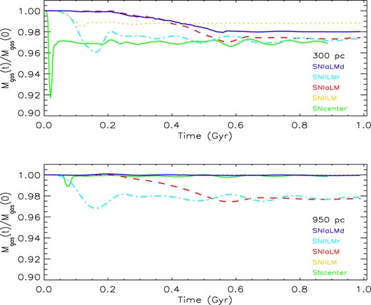
Mass fraction as a function of time inside two different galactic regions (300 pc, upper panel and 950 pc, bottom panel) for the five simulations with 10 000 SNe: SNcenterT0: solid line, SNIILM: dotted line, SNIaLM: dashed line, SNIILMr: long-short dashed line, SNIaLMd: dot –dashed line.
3.2 10 000 SNe II distributed in time and space
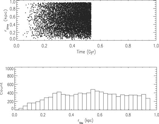
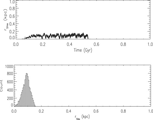
The second step in the analysis of the effects of the spatial and temporal distribution of the SNe in the gas dynamics of the dSphs is performed by adopting the same number of SNe as in the previous case (10 000 SNe), but considering all of them as SNe II (Simulation SNIILM). The number of SNe as a function of time is given by the SNe rate taken from the chemical evolution model of Lanfranchi & Matteucci (2007), and their distribution in time is controlled by the prescription described in Section 2.2: the position where each SN occurs is random, weighted by the density (see Caproni et al. 2015 for more details). The first consequence of the adopted SNe rate is the interval between the beginning of the simulation and the explosion of the first SNe: 15 Myr. This is approximately the time-scale required for gas to collapse and form the first stars, and for a massive star to go through its evolution and explode as an SN. Following the gas density distribution, all SNe occur within a distance of 100 pc from the centre in the initial 20 Myr (Fig. 4, upper panel). As the gas moves to outer regions of the galaxy, increasing locally the gas density, the new SNe start to explode farther from the centre. After a hundred Myr, all 10 000 SNe II are distributed within a |$\sim$|150 pc radius region (Fig. 4).
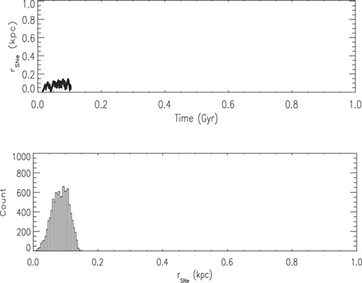
Spatial distribution of all 10 000 SNe II in simulation SNIILM.Upper panel: distance in kpc to the centre of the galaxy of all SNe as a function of time. Lower panel: number of SNe in each bin of distance to the centre of the galaxy.
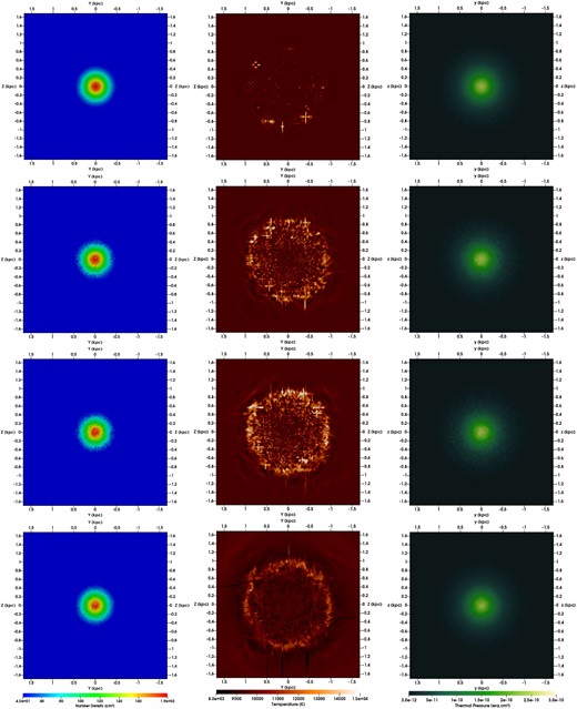
The spatial distribution of SNe is determined by the gas density profile, which is influenced by the energy that SNe release into the ISM: the energy of the SNe moves the gas changing its density distribution, that, on the other hand, defines where new SNe will occur. Before the first 30 Myr, the injection of energy by the first SNe heats only limited regions around the explosions, decreasing the gas density locally to half the inital central density (|$\rho \sim$| 1.66 |$\times$| 10|$^{-22}$| g cm|$^{-3}$|), moving the gas outwards the central region, and creating a shell of higher density (|$\rho \,\, \sim$| 3.65 |$\times$| 10|$^{-22}$| g cm|$^{-3}$|) and temperature (around 1.55 |$\times$| 10|$^4$| K) (Fig. 5, upper panels). Regions off the centre with higher density appear in different points of the galaxy followed by new SNe. The SN remnants exhibit limited interaction with each other due to the distance among them, but non-spherical shockwaves mix the gas of the galaxy, increasing the global temperature of the ISM. After 80 Myr, the temperature of the central region has increased to 1.0 |$\times$| 10|$^4$| K with peaks of 1.8 |$\times$| 10|$^4$| K, almost no region with the highest gas densities can be seen in the centre of the galaxy (Fig. 5, second panels from above), and regions with the lowest gas density are created after |$\sim$|100 Myr: |$\rho \,\, \sim$| 1.49 |$\times$| 10|$^{-22}$| g cm|$^{-3}$| (almost 60 |${{\ \rm per\ cent}}$| of the initial value). After around 140 Myr, the rate of SNe starts to decrease, gravity pulls back gas to the centre of the galaxy and the central gas density increases again. The gas temperature starts decreasing slowly, but there are still regions with tempertures as high as 1.3 |$\times$| 10|$^4$| K and shockwaves continue heating the gas of the ISM far from the centre of the galaxy (Fig. 5, bottom panels). The limited number of SNe, their wide dispersion, and the high gas density in the centre of the galaxy, where most SNe II occur, likely contribute to the minimal impact of these explosions on the ISM. While localized effects on temperature and gas density are observed, the overall properties of the ISM remain largely unchanged.
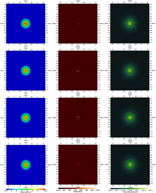
Cut in the |$x = 0$| plane for the gas density (left), gas temperature (center), and thermal pressure (right) of the gas at t = 30 Myr (upper), 80 Myr (second panel), 140 Myr (third panel), and 300 Myr (bottom) for the simulation SNIILM.
The gas mass fraction computed in two different regions of the galaxy reflects the changes in the density due to the gas flow. In Fig. 3, the fraction of initial gas that remains inside two different galactic regions as a function of time (300 pc, upper panel and 950 pc, bottom panel) is represented by the orange dotted line for simulation SNIILM. From 50 Myr, one can observe a marginal decrease (lower than 2 |${{\ \rm per\ cent}}$|) in the mass fraction inside the central region (within 300 pc) that keeps going until 120–130 Myr (when SNe stop exploding). After that, gravity pulls back a fraction of the gas to the centre keeping the gas mass constant until the end of the simulation at 1 Gyr. When the whole galaxy, up to its tidal radius, is considered, no substantial change in the gas mass can be noticed: it remains almost constant, close to 100 |${{\ \rm per\ cent}}$|. No blown out is detected. In contrast to the previous scenario, the initial mass-loss is less severe, but due to the distribution of the explosions over time, there is no return of gas to the centre of the galaxy. Gas is indeed removed from that region. This finding emphasizes the significance of incorporating SNe time-scales into galaxy evolution simulations over extended periods (from hundreds of Myr to Gyr).
3.3 10 000 SNe Ia distributed in time and space
In this work, it was adopted, for the first time, the SNe rates of Type II and Type Ia from a chemical evolution model with a detailed prescription for the occurrence of Type Ia SNe, including the lifetimes of both the primary and secondary stars in the binary system (Matteucci & Greggio 1986; Lanfranchi & Matteucci 2007). Normally the differences in the time-scale and spatial distribution between SNe II and SNe Ia are not considered in hydrodynamic simulations aiming to investigate the effects of stellar feedback in galaxies and in the gas loss. In order to investigate the effects of a proper consideration of SNe Ia in the gas dynamics of a classical dSph, we run a simulation with the exactly same initial set-up and physical conditions as the previous one, but adopting only the feedback from 10 000 SNe Ia (simulation SNIaLM).
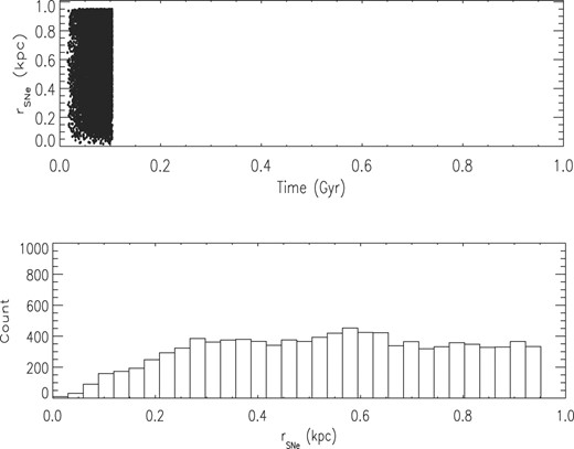
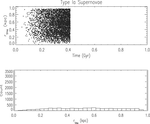
Due to the differences in the SNe time-scales and the prescription adopted in our simulations for the sites of the injection of the energy from SNe Ia, the distributions in time and space of the two types of SNe differ considerably. The number of SNe Ia that occur before 100 Myr (period during which almost all ten thousand SNe II already exploded) is low (only 27 explosions). This number, however, increases until almost 540 Myr, when it reaches the 10 000 SNe. SNe Ia also occur anywhere in the galaxy up to its tidal radius (upper and lower panels on Fig. 6), contrary to the SNe II that are concentrated inside a region of 200 pc radius. This difference allows us to study the gas dynamics when the energy injected by the SNe in the medium is distributed over longer scales of time and space. By doing that we can check whether the gas loss depends mainly on the total energy released in the medium or on how this energy is released over space and time.
Spatial distribution of all 10 000 SNe Ia in simulation SNIaLM. Upper panel: distance in kpc to the centre of the galaxy of all SNe as a function of time. Lower panel: number of SNe in each bin of distance to the centre of the galaxy.
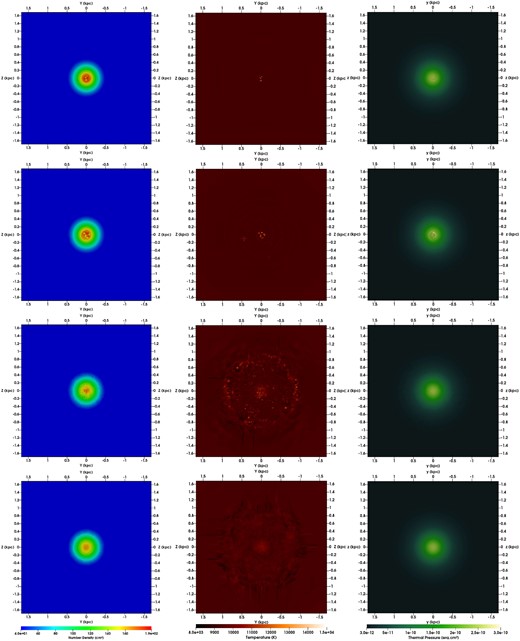
The longer SNe Ia time-scale and the fact that these explosions are not confined to the galaxy’s core but can occur anywhere within it reflect directly on how the gas density, temperature, and pressure evolve. The first 30 SNe Ia take almost 100 Myr to explode, at very dispersed locations in the galaxy (top panels on Fig. 7), causing a negligible effect on the ISM. Important effects on the gas density, on the temperature, and on the pressure can be noticed only when more than 300 SNe Ia occurred, after 180 Myr (second line on Fig. 7). The gas density profile reveals regions of diluted gas at radii exceeding 200 pc. Slower than in the simulation SNIILM, the density in the central region decreases as the galaxy evolves. The outer regions also exhibit a decrease in gas density, in contradiction with the scenario where only SNe II are considered. In conjunction with the density decrease, the gas temperature profile reveals the heating of the gas, especially at larger galactic radii, reflecting very well the SN Ia explosions. This heating, however, is more intense due to the lower density of the gas. A few points of high temperature can be seen inside a 200 pc radius from the centre, revealing the few SNe that exploded centrally before 180 Myr. After 390 and 510 Myr (third and last lines in the middle of Fig. 7), gas in the outer regions (> 600 pc) reaches temperatures of an order of 1.0 |$\times$| 10|$^4$| K (with peaks as high as 1.55 |$\times$| 10|$^4$| K), and more regions of high temperature can be observed in the central region of the galaxy.
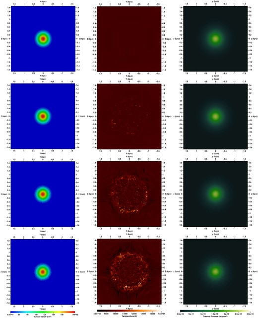
Cut in the |$x = 0$| plane for the gas density (left), gas temperature (centre), and thermal pressure (right) of the gas at t = 80 Myr (upper), 180 Myr (second panel), 390 Myr (third panel), and 510 Myr (bottom) for the simulation SNIaLM.
The heating of the gas and its density profile can explain how it is removed from the galaxy when only SNe Ia are adopted in the simulations. The fraction of the initial gas mass as a function of time that remains inside two spherical regions with different radii for the simulation SNIaLM is displayed by the red dashed line on Fig. 3 (300 pc, upper panel and 950 pc, bottom panel). Contrary to the case with only SNe II, the mass fraction remains constant for almost 200 Myr due to the low number of SNe Ia. After that, it starts decreasing slowly. The decrease lasts for almost 300 Myr, reaching almost 97 |${{\ \rm per\ cent}}$| of the initial gas mass inside a 300 pc radius. This value remains constant until the end of simulation. The final mass in this region is very similar to the one in the case SNIILM. The later and slower decrease compared to simulation with only SNe II can be explained by the SNe Ia time-scale. They take longer to begin exploding and also exhibit a lower rate. However, when regions at larger radii are also included in the gas loss analysis, the scenario changes considerably comparing to the one with only SNe II. The gas evolution inside a 950 pc radius region exhibits exactly the same trend as in the case of the central region: the gas loss is marginally lower (around 0.5 |${{\ \rm per\ cent}}$| lower). This pattern is quite different from the one observed when in simulation SNIILM: no gas loss is reported inside 950 pc. One can see, comparing Figs 5 and 7, that in the SNIaLM case not only the central gas but also gas in the outskirts of the galaxy is heated, and even more intensely. The heated gas in the outer regions gains higher speed and leaves the galaxy easier than the central gas, diminishing the total initial gas fraction in the galactic ISM.
The comparions of the orange dotted and red dashed lines on Fig. 3 suggest clearly that when the same number of each type of SNe is considered separated, the SNe Ia are more efficient in removing gas of the galaxy. Two basic differences can play a role in the gas removal in each case: the spatial and temporal distributions. Which of these two factors, however, are more important in the more intense gas loss? We adopted two alternative prescriptions to investigate whether temporal or spatial distribution is more important. We maintained the SNe rate of each SN type but changed the prescriptions for the sites for their explosion in simulations SNIILMr and SNIaLMd. The results are discussed in the next two sections.
3.4 10 000 SNe II randomly distributed in space
In simulation SNIILMr, we adopted the same initial set-up and same physical conditions of simulation SNIILM but with a different prescription for the sites where the energy of SNe II is injected. In the SNIILMr simulation, SNe II can occur anywhere in the galaxy: the choice of the computational cell does not depend on the gas density. Consequently, all 10 000 SNe II are dispersed across the entire galaxy (Fig. 8). This differs from the SNIILM scenario, where all SNe II are concentrated within a 150 pc radius at the galaxy’s core. By comparing these two simulations, we can infer the role played by the spatial distribution of the SNe in the gas loss.
Spatial distribution of all 10 000 SNe II in simulation SNIILMr. Upper panel: distance in kpc to the centre of the galaxy of all SNe as a function of time. Lower panel: number of SNe in each bin of distance to the centre of the galaxy.
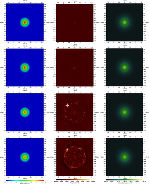
Soon at the beginning of the evolution of the galaxy (at 30 Myr), the first SNe II events influence the temperature of the galactic gas also in regions far from the centre of the system (Fig. 9, top panel of the middle column). When the energy from a few isolated SNe is released in the medium, the neighbouring gas is heated to 1.3–1.5 |$\times$| 10|$^4$| K and small regions with temperature higher than its surroundings appear in the galaxy. This situation is comparable to what’s observed in the simulation SNIaLM but in a much faster time-scale. In Fig. 7, one can notice that the SNe start heating the gas only after around 180 Myr, whereas in SNIILMr the gas at large galactic radii (>600 pc) is almost totally heated (T> 1.1 |$\times$| 10|$^4$| K with peaks up to 1.4 |$\times$| 10|$^4$| K) ealier, already at 100 Myr. The impact of the SNe on the external regions of the galaxy can also be observed in the profile of the gas density (left column of Fig. 9). At 30 Myr it is possible to observe a decrease in the gas density in small regions at |$\sim$|200 pc from the Galactic Centre. This decrease reaches its peak at around 110 Myr, both in the external and central regions, when all the 10 000 SNe already exploded. After that, no substantial changes occur.
Cut in the |$x = 0$| plane for the gas density (left), gas temperature (center), and thermal pressure (right) of the gas at t = 30 Myr (upper), 80 Myr (second panel), 100 Myr (third panel), and 140 Myr (bottom) for the simulation SNIILMr.
The gas loss rate follows the same temporal pattern in both regions analysed. There is a decrease in the initial fraction of the gas mass that remains inside the galaxy until approximately 170 Myr, remaining almost constant after that (cyan long-short dashed line on Fig. 3). This decrease is due to the energy injected in the medium by the 10 000 SNe that occur all almost in the same epoch, before 110 Myr. Since the SNe, in this case, are distributed all over the galaxy, gas is lost in both regions, inner and outer, at very similar fractions: 2 |${{\ \rm per\ cent}}$| and 2.5 |${{\ \rm per\ cent}}$| of the initial gas mass at 950 and 300 pc, respectively. Compared to previous simulations, in the case SNIILMr more gas is retained than when only SNe Ia are considered. In such a scenario, the SNe Ia events are distributed throughout the galaxy but over a longer time-scale (85 |${{\ \rm per\ cent}}$| to 90 |${{\ \rm per\ cent}}$| inside 950 pc and 70 |${{\ \rm per\ cent}}$| and 75 |${{\ \rm per\ cent}}$| at 300 pc). On the other hand, in simulation SNIILM, with the SNe concentrated in central dense region, almost no gas is lost in the outer region, but the same amount of gas inside the central 300 pc is roughly retained in the SNIILM and SNIILMr cases. This suggests that when the stellar feedback occur also at larger galactic radii more gas is loss. The outer SNe inject the same amount of energy in the ISM but in less dense medium, in a region with a shallower gravitational potential. Less dense gas gains more speed and, being in outer regions, escape the galaxy easier. Central gas, however, transfers its energy to the surrounding medium and loses energy in its way across the galaxy.
3.5 10 000 SNe Ia in denser regions
In previous section, the dependence of the gas loss on the spatial distribution of the SNe was examined by considering only SNe II, exploding across the galaxy in a short time-scale. On the other hand, the effects of the temporal distribution are analyzed in simulation SNIaLMd by assuming 10 000 SNe Ia, with the same initial conditions of all other previous simulations, but with a different prescription for the sites of energy injection: the regions with higher gas densities are favored to host a SN Ia explosion. By doing that, the 10 000 SNe explode inside a spherical region of a radius around 200 pc, but in a time-scale of almost 550 Myr (Fig. 10). This is the time-scale required in the chemical evolution models to form and evolve the stars that give rise to all 10 000 SNe, considering the stellar lifetimes from Padovani & Matteucci (1993).
Spatial distribution of all 10 000 SNe Ia in simulation SNIaLMd. Upper panel: distance in kpc to the centre of the galaxy of all SNe Ia as a function of time. Lower panel: number of SNe Ia in each bin of distance to the centre of the galaxy.
The effects in the gas density, temperature, and pressure can be easily compared to the simulation SNIaLM, in the sense that the time intervals during which SNe are occuring are similar in both. The first SNe occur almost isolated and do not impact the ISM in a significant way, nor its density neither its temperature. It is only after around 80 Myr that the first signs of the SNe in the ISM can be noticed, but their impact is restricted to the central region of the galaxy, and very spacely restricted. The density in the vicinity of the explosions decrease only marginally and the temperature increases to almost 1.1 |$\times$| 10|$^4$| K. At around 180 Myr, filaments wiht low densities (84 |${{\ \rm per\ cent}}$| of the initial value) are created in the inner 130 pc, whereas outside 250 pc radius there is almost no change in the gas density. Only the shock waves can be noticed. At the end of the simulation, at 1 Gyr, the mean density inside a 200 pc radius decreased to almost 80 |${{\ \rm per\ cent}}$| the initial central value. The temperature on the other hand increased from around 7000 K to approximately 1.05 |$\times$| 10|$^4$| K.
Following the low SNe rate, the fraction of the initial gas that is expelled from the regions examined (300 pc, upper panel and 950 pc, bottom panel in Fig. 3, blue dot–dashed line) is low in the first 200 Myr: there is almost no gas loss. As the evolution proceeds, the number of SNe increases in the central region of the galaxy and the amount of gas starts to decrease locally, but slower than in the SNIILM case. Gas continues to be expelled from the central region at an almost constant rate until almost 550 Myr, when the fraction of the initial gas reaches its lowest value (|$\sim 98{{\ \rm per\ cent}}$|) and all 10 000 SNe already exploded. This value remains constant until the end of the simulation. When all the region inside the tidal radius of the galaxy is considered, the removal of gas is almost negligible, it remains the same as the initial one.
3.6 50 000 SNe types II and Ia
The findings presented in the preceding sections clearly indicate that SNe II and SNe Ia, when analysed independently in simulations, exert differing influences on gas expulsion in dSphs. The fact that SNe Ia explode everywhere in the galaxy and over an extended time-scale seems to favour the gas loss. To make sure that indeed this is the case, both SN types should be considered together, as it is done on two simulations with the same set-up as the previous ones, but with a higher total number of SNe (50 thousand in each), and different fractions of SNe II and SNe Ia in each one. In the simulation SN4505LM, 45 000 SNe II and 5000 SNe Ia are adopted whereas in simulation SN3020LM 30 000 SNe II and 20 000 SNe Ia are taken into account. The choice of the relative number of each type of SNe on SN4505LM resides on the fact that LM07 models predict roughly nine times more SNe II than SNe Ia, so this simulation is the fiducial one in this section. In SN3020LM, the number of SNe Ia is increased, to investigate how their energetic feedback impacts the gas loss, and the SNe II is decreased in an amount that maintains the same total number of SNe in both simulations. The rates of SNe II and SNe Ia are the same as in the chemical evolution models of Lanfranchi & Matteucci (2007), but the SN explosions are halted when the maximum number of each SN type is achieved. It should also be reminded that since the total number of SNe in these two simulations is five times higher than in the previous sections, they cannot be compared to any of the previous simulations. They are comparable only with each other.
The first clear difference between simulations SN4505LM and SN3020LM is the total time interval during which SNe explode and energy is injected by them in the medium. This time interval is determined mostly by the SNe Ia time-scale. Besides this temporal difference, the prescriptions for the sites of occurrence of each type of SNe give rise to different spatial distribution of SNe II and SNe Ia. When simulations SN4505LM and SN3020LM are compared, the time and spatial distributions of SNe Ia exhibit significant differences. In the case of SNe II, both the time interval during which they explode and the galactic region where they occur are similar in the two simulations (Figs 11 and 12). The fact that the maximum numbers of these SNe are not that different (45 000 and 30 000) and that they have a short time-scale, allied to the fact that they explode in denser regions, give rise to a concentrated distribution in both scenarios. In simulation SN4505LM, the 45 000 SNe II explode inside a spherical region of |$\sim$|200 pc radius before 210 Myr, whereas the 30 000 SNe II in simulation SN3020LM take almost 175 Myr to end completely, all of them within a spherical region with a radius of 180 pc. On the other hand, when the distributions of SNe Ia are examined, the differences between the two simulations are much more evident (Figs 13 and 14). The 5000 SNe Ia from simulation SN4505LM start exploding at around 30–50 Myr and keep injecting energy in the medium until 400 Myr, a much wider time-scale than for SNe II, but narrower than the one for the 20 000 SNe Ia in simulation SN3020LM. These take almost 730 Myr to cease. Besides the wider spread in time, SNe Ia inject energy throughout the galaxy, often reaching the tidal radius. As a consequence, in simulation SN3020LM the same amount of energy is released in the medium as in SN4505LM, but during a much longer time-scale (730 Myr compared to 400 Myr) and with a large fraction of the total energy being injected in regions far away from the centre of the galaxy (up to 950 pc).
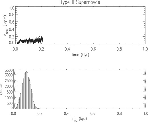
Spatial distribution of all 45 000 SNe Ia in simulation SN4505LM. Upper panel: distance in kpc to the centre of the galaxy of all SNe as a function of time. Lower panel: number of SNe in each bin of distance to the centre of the galaxy.
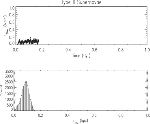
Spatial distribution of 30 000 SNe II in simulation SN3020LM. Upper panel: distance in kpc to the centre of the galaxy of all SNe as a function of time. Lower panel: number of SNe in each bin of distance to the centre of the galaxy.
Spatial distribution of all 5000 SNe Ia in simulation SN4505LM. Upper panel: distance in kpc to the centre of the galaxy of all SNe as a function of time. Lower panel: number of SNe in each bin of distance to the centre of the galaxy.
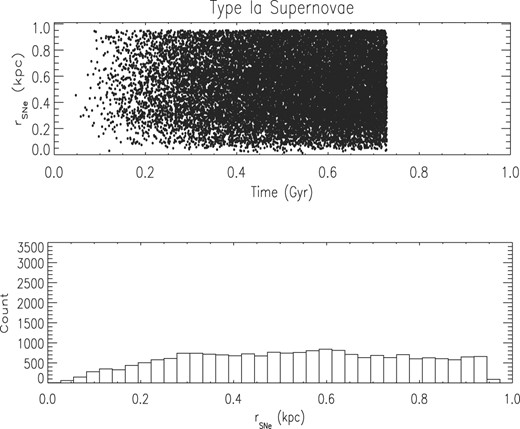
Spatial distribution of all 20 000 SNe Ia in simulation SN3020LM. Upper panel: distance in kpc to the centre of the galaxy of all SNe as a function of time. Lower panel: number of SNe in each bin of distance to the centre of the galaxy.
The combined energy input from SNe II and SNe Ia significantly affects the gas dynamics within both the central and outer regions of galaxies during both early and late stages of their evolution. The relative number of each type of SNe, however, is crucial in determining the fate of the interstellar gas. When the fraction of SNe II is much higher than the one of SNe Ia (simulation SN4505LM), similar to what is adopted in chemical evolution models that reproduce the chemical properties of several local dSphs, the effects on the gas dynamics and on the evolution of the gas content are concentrated in the central region of the galaxy and in the early galactic ages. The first SNe II start exploding a few Myr (around 15 Myr) after the beginning of the simulation at the centre of the galaxy (first line in Fig. 15). At 40 Myr, filaments of high temperature (12400 K, 1.3 times higher than the surrounding medium) and low density (|$\rho = 2,32 \times 10^{-22}$| g cm|$^{-3}$|, 23|${{\ \rm per\ cent}}$| lower than in the vicinity) are created. The shock-waves due to the SN remnants propagate outwards decreasing slightly the central gas density and rising its temperature. This new region of lower density and higher temperature expands from 40 pc to around 90 pc between 40 and 100 Myr. Signs of SNe feedback can also be noticed in the gas temperature profile not only in the Galactic Centre, but at distances as large as 500 pc. As the galaxy evolves, the number of SNe Ia increases and their feedback at more external regions of the galaxy becomes increasingly important. The temperature of the gas, at 300 Myr, reaches peaks of 11 500 K in several locations on the outskirts of the galaxy, whereas in more central regions it gets as high as 11 000 K (third line, central column Fig. 15) due to the predominant effects of SNe II. After the feedback of both types of SNe ceases, both the external and central regions of the galaxy maintain a mean temperature of |$\sim$|10 000 K.
Cut in the |$x = 0$| plane for the gas density (left), gas temperature (centre), and thermal pressure (right) of the gas at t = 40 Myr (upper), 100 Myr (second panel), 300 Myr (third panel), and 600 Myr (bottom) for the simulation SN4505LM.
The gas density distribution, on the other hand, is not significantly affected after all SNe occurred. At 300 Myr, the profile of the gas density is very similar to the initial one from the centre of the galaxy to |$\sim$|400 pc. Filaments of lower density, however, can be noticed at locations |$\sim$|100 pc far from the Galactic Centre; a clear effect of SNe Ia that explode isolated in space and time. Due mostly to the effects of gravity, at 600 Myr the gas density is even more homogeneous than previously with values differing a factor of almost two from the centre of the galaxy to a galactic radius of 300 pc (|$\rho = 1.5 \times 10^{-22}$| g cm|$^{-3}$| to |$\rho = 2.8 \times 10^{-22}$| g cm|$^{-3}$|, respectively). Note that even the central density is lower than the one at 40 Myr and 16 |${{\ \rm per\ cent}}$| lower than the initial central density. The same behaviour is observed in the thermal pressure (last column of Fig. 15): the SNe feedback decreases the overall gas pressure in the Galactic Centre, eliminating the highest values estimates at the beginning of the evolution of the galaxy.
A higher fraction of SNe Ia (as adopted in simulation SN3020LM), on the other hand, affects the medium over a longer time-scale and at more external regions. Early in the evolution of the galaxy differences can be noticed in the gas density, temperature, and thermal pressure distributions: at 40 Myr (first line of Fig. 16, left, middle, and right columns, respectively) a few spots of lower density (from 31 |${{\ \rm per\ cent}}$| to 25 |${{\ \rm per\ cent}}$| lower than the surroundings), higher temperature (10 600 and 12 600 K) and lower pressure are created around the centre of the galaxy (within a radius of 100 pc). As the evolution proceeds, these regions increase in number and size (from tens to hundred pc) due to the various shock-waves created by subsequent SN explosions. Simultaneously, new SNe explode diluting the region of high gas density and increasing the gas temperature (up to |$\sim$|12 200 K) at the centre of galaxy. At 100 Myr, a few SNe Ia can be seen in the outer regions of the galaxy: isolated regions with high temperatures (11 000 K) at distance as large as 400 pc from the centre. As the galaxy evolves, more SNe (of both types) explode heating the gas, that reaches peaks of 11 600 K at the tidal radius at 300 Myr and 10 800 K at 900 Myr. In the centre, after all SNe are halted, the gas temperature oscilates from 9400 to 10 300 K. The gas density at the centre of the galaxy, on the other hand, descreases only a few per cent (|$\sim$|6 |${{\ \rm per\ cent}}$| during the same time interval (from 300 to 900 Myr).
Cut in the |$x = 0$| plane for the gas density (left), gas temperature (centre), and thermal pressure (right) of the gas at t = 40 Myr (upper), 100 Myr (second panel), 300 Myr (third panel), and 600 Myr (bottom) for the simulation SN3020LM.
The amount of gas that is lost as a function of time is analysed in the two simulations (SN4505LM: solid lines and SN3020LM: dotted lines in Fig. 17) inside two different regions, a central one with a radius of 300 pc (black lines in Fig. 17) and another one inside approximately the tidal radius of the galaxy (950 pc)(red lines in Fig. 17). In the first 200 Myr, the gas loss exhibits identical patterns in both simulations in both regions, due to the major role played by the SNe II in early stages of the galactic evolution. Since these SNe occur more concentrated in the central region, the gas loss inside the 300 pc radius is higher (more than 2 |${{\ \rm per\ cent}}$|), whereas it is negligible inside the 950 pc radius. After that initial phase, one can notice from 200 Myr until 450 Myr a slower decrease in the remaining gas fraction inside the central region (black lines in Fig. 17) in the SN3020LM case when compared to the simulation SN4505LM, due to the higher fraction of SNe II that occurred in the later simulation. When the whole galaxy, up to its tidal radius, is considered, there is no difference until 450 Myr. It is around this epoch that both types of SNe cease to explode in SN4505LM, keeping the gas fraction almost constant from that moment to the end of the 1 Gyr in both regions with |$\sim 97{{\ \rm per\ cent}}$| in the 300 pc region and |$\sim 99{{\ \rm per\ cent}}$| in the 950 pc region. The higher number of SNe Ia in SN3020LM leads to a more prolonged effect of their feedback in the ISM decreasing even more the fraction of the initial mass in central and external regions, reaching at the end of the simulation |$\sim 95{{\ \rm per\ cent}}$| in the 300 pc region and |$\sim 97{{\ \rm per\ cent}}$| in the 950 pc region. In both scenarios, the gas loss is more intense in the central region than in the more extended one.
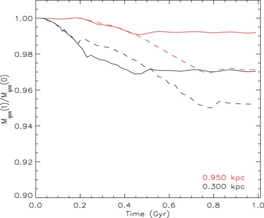
Mass fraction as a function of time inside two different galactic regions (300pc, bottom lines and 950 pc, top lines) for the simulations SN4505LM (solid lines) and SN3020LM (dotted lines).
4 DISCUSSION AND CONCLUSIONS
We investigated the effects of SNe explosions in the dynamics of the ISM in a classical dSph taking into account SNe rates (of Types II and Ia) from chemical evolution models that reproduce very well the chemical properties of several local dSphs. These models consider properly the stellar lifetimes, resulting in different time-scales for the occurrence of SNe II and SNe Ia and very distinct SNe rates: whereas SNe II rate follows closely the star formation rate (all SNe occur within 3 Gyr of evolution with a peak around 400 Myr), the rate of SNe Ia does not exhibit a clear peak and maintains a plateau from 0.8 to 1.5 Gyr. Due to the distinct time-scales for the occurrence of SNe II and SNe Ia, the prescriptions for the sites where the energy of each type of SN is injected in the hydrodynamic code are not the same: whereas SNe Ia can explode everywhere in the galaxy (the choice of the computational cell is totally random), the cells with the highest gas density are the ones favoured to host an SN II explosion. By doing that, we are able to infer the contribution of these two types of SNe for the gas removal in a typical dSph and also discuss the importance of the temporal and spatial distribution of SNe in the gas loss of the system. We restrict the number of SNe to 50 000 in total and simulated the gas dynamics for 1 Gyr in the sake of computational capacity.
We ran seven simulations: the first simulation considered only SNe II (simulation SNIILM) and the second one only SNe Ia (simulation SNIaLM), 10 000 SNe in each. The 10 000 SNe II occur more clustered (they all explode inside a central 150 pc radius) and all before 110 Myr, whereas SNe Ia are distributed throughout the galaxy, often reaching distances of up to 950 pc, and have significantly longer explosion time-scales, almost 550 Myr. These two differences result in very distinct gas loss rates.
In the case SNIILM, no gas is lost from inside a spherical region of 950 pc radius (similar to the tidal radius of Ursa Minor galaxy) due to the limited region and short time-scale where the energy from SNe is injected. Only 1 |${{\ \rm per\ cent}}$| of the inital mass content is expelled from the 300 pc central region, but it does not gain enough energy to escape the galactic potential well. After the majority of SNe explode, there is a slight decrease in the gas mass inside 300 pc, reaching less than 99 |${{\ \rm per\ cent}}$| of the initial mass. In the simulation with only SNe Ia, on the other hand, gas is removed slower, as a consequence of the lower SNe Ia rate and its longer time-scale. From the central 300 pc, the amount of gas removed at the end of the 1 Gyr is higher than the one in simulation with only SNe II, around 2.5 |${{\ \rm per\ cent}}$|, but SNe Ia alone are much more efficient in removing the gas of the whole galaxy when compared to the SNe II. Inside a 950 pc radius, the gas fraction starts decreasing substantially at 200 Myr and maintains an almost constant rate of gas loss until the end of all explosions around 550 Myr, reaching 98 |${{\ \rm per\ cent}}$| of the initial gas mass. Besides the particular time-scales and rates, the differences in the gas removal are related to the spatial distribution adopted for the SNe Ia on the simulation: they can occur everywhere in the galaxy. When the energy is released in outer regions of the galaxy, gas is removed easier. When the gas density is lower, gas particles gain more energy and reaches higher speed, becoming able to escape the gravitational potential well of the galaxy.
To further explore the relative importance of spatial and temporal SN distributions on gas loss, we conducted two additional simulations replicating the configurations of our previous models, but changing the prescriptions for the choice of the cell where SNe can occur. In simulation SNIILMr, SNe II are allowed to explode completely random in all galaxy within the tidal radius, whereas in SNIaLMd SNe Ia must occur preferentially in the cells with the highest gas density. These choices result in two new scenarios: one in which all energy from the 10 000 SNe is injected before 110 Myr all over the galaxy, including regions at large galactic radii, and another one with the SNe clustered in the central 200 pc with the energy being injected during a much longer time interval, up to 550 Myr. The results suggest that the spatial distribution has a stronger impact in the gas loss when the whole galaxy is examined. At the end of the simulation SNIaLMd, 2 |${{\ \rm per\ cent}}$| of the initial gas mass is removed from the spherical region with 950 pc radius, whereas no gas is lost in the case SNIILMr. In the central region, less gas is removed also in the case when the SNe are clustered but diluted in time, but the difference is lower: almost 2 |${{\ \rm per\ cent}}$| versus 2.5 |${{\ \rm per\ cent}}$|. One can conclude that clustered SNe are effective in expelling the gas out of the central region when they explod for a longer time interval, but not able to remove the gas of the galaxy. On the other hand, when the SNe can inject energy everywhere inside the tidal radius, gas from the whole galaxy are easier removed.
We can also compare the effects of the temporal distribution of the SNe by comparing simulations SNIILM with SNIaLMd and SNIaLM with SNIILMr. When the SNe are clustered in the central 200 pc region, but diluted in time (up to 550 Myr), the fraction of gas removed from the central region is two times higher compared to when they all explode before 110 Myr. When they are allowed to explode randomly in the galaxy there is also a higher gas loss when they explode in a longer time interval: 2.8 |${{\ \rm per\ cent}}$| inside 950 pc and 2.2 |${{\ \rm per\ cent}}$| inside 300 pc of the gas is lost in this case, compared to 2.4 |${{\ \rm per\ cent}}$| and 2 |${{\ \rm per\ cent}}$|, respectively, when all SNe release their energy before 110 Myr.
Finally, two last simulations were performed, each with a total of 50 000 SNe of both types, but with different fractions of each one: SN4505LM with 90 |${{\ \rm per\ cent}}$| of SNe II and 10 |${{\ \rm per\ cent}}$| of SNe Ia and SN3020LM with 60 |${{\ \rm per\ cent}}$| of SNe II and 40 |${{\ \rm per\ cent}}$| of SNe Ia. By comparing one with another, it becomes clear that indeed the SNe Ia favour the gas loss, in contrast to results that argue that clustered SNe favour the gas loss (Fielding et al. 2017; Gentry et al. 2017, 2019; Fielding; Quataert & and Martizzi 2018; Martizzi 2020; Schneider et al. 2020; Gutcke et al. 2021; Smith et al. 2021). Besides the fact that we consider a spheroidal system (dSph) whereas all these works simulate disc galaxies, the majority of them differs from our simulations in three main points: the time-scale of the simulation, the consideration of SNe Ia, and the particular time-scale and rate of the SNe Ia. As described before, clustered SNe (SNe II in our case) only favour the mass-loss in central regions of the galaxy and in short time-scales. When the whole galaxy over a Gyr time-scale is considered, the effect of clustered SNe is diminished considerably. After SNe II cease to explode, gravity pulls back the gas to the centre of the galaxy and the fraction of the initial gas that is indeed lost is low. SNe Ia, on the other hand, have a much longer lifetime and hence can explode all over the galaxy for several hundred of Myr. The continuous launch of energy in the medium keeps the ISM at high temperatures and low densities for a long period, preventing the gas to fall back due to gravity. At the same time, when SNe Ia inject energy in the outskirts of the system, the gas is easier blown out from the tidal radius and does not fall back. When both types of SNe are considered, the case with a higher fraction of SNe Ia exhibits a higher gas loss and at the end of 1 Gyr and the remaining gas inside the galaxy (within a 950 pc radius) is lower. A similar conclusion was reached by Ceverino & Klypin (2009): isolated stars (or runaway stars) facilitate the feedback. In their case, when one of the stars in a massive binary system becomes an SN the companion can be ejected from molecular clouds moving up to 100 pc away from molecular clouds before exploding as SN. By performing cosmological simulations with very high resolution (better than 50 pc) with this effect implemented, these authors found substantial outflows with speeds as high as 1000–2000 km s|$^{-1}$| in forming and active galaxies.
It is safe to argue, then, that stellar feedback from both types of SNe should be taken into account in hydrodynamic simulations, with the differences in the time-scale for these two types properly considered, together with the spatial distribution. Several works do not distinguish Types II and Ia SNe (Mac Low & Ferrara 1999; Ferrara & Tolstoy 2000; Wada & Venkatesan 2003) and those that do it, do not treat in details the SNe Ia. Even in the first works of the group (Caproni et al. 2015, 2017) such distinction were note addressed. Recchi, Mattuecci & D’Ercole (2001), Recchi et al. (2002), Melioli & de Gouveia Dal Pino (2004), and Marcolini et al. (2006), for instance, already pointed out the importance of SNe Ia in the gas removal and enrichment in dwarf galaxies. Since SNe Ia take a longer time to explode, their energy is injected in a already diluted and heated medium, imprinting more kinetic energy in the gas, which would leave the galaxy easier. That would also change the enrichment of the gas, since these two types of SNe contribute with different amount of mass of different chemical species. The heated gas released by SNe Ia could leave easier the galaxy enriching the galactic wind with Fe-peak elements, argued Recchi, Matteucci, D’Ercole (2001) and Recchi et al. (2002). Marcolini et al. (2006), on the other hand, suggested that stars with low values of [|$\alpha$|/Fe] could be formed in regions next to site of explosions of SNe Ia, which would be rich on Fe. These works however did not distinguished the sites for the injection of types Ia and II SNe.
Besides that, whereas Wada & Venkatesan (2003) incorporated gas self-gravity, our simulations do not consider it. Given the dominance of the cored DM potential over the luminous matter potential, gas self-gravity is unlikely to substantially alter our results regarding the gas loss from the entire galaxy. In the galaxy’s central regions, on the other hand, where gas mass should predominate it could be important. However, our simulations lack the large-scale cavities that could destabilize the galaxy, minimizing the importance of gas self-gravity. In fact, it could hinder gas removal by SNe II, as gas could be concentrated near the galaxy’s centre, potentially leading to a more clustered distribution of SNe II than observed in our simulations. That should be tested in posterior simulations adopting gas self-gravity. Given that, our results suggest strongly that the sites were the energy is inserted, if the SNe are clustered or not, and the temporal distribution of the SNe play a significant role in the gas dynamics and should be addressed with care when stellar feedback is investigated.
ACKNOWLEDGEMENTS
This work has made use of the Sistema de Computação Petaflópica do SINAPAD - Laboratório Nacional de Computação Científica (LNCC - http://sdumont.lncc.br). The authors thank the Brazilian agency CNPq (grant 304928/2015-1) and FAPESP (grants 2014/11156-4, 2017/25651-5, 2017/25799-2, and 2019/21615-0).
ParaView (Ahrens & Law 2005, Ayachit 2015), IDL (Interactive Data Language, https://www.harrisgeospatial.com/Software-Technology/IDL).
DATA AVAILABILITY
The data underlying this article will be shared on reasonable request to the corresponding author.
