


ABSTRACT
Recently inaugurated telescopes, such as the MeerKAT radio telescope and the upcoming Rubin Observatory Legacy Survey of Space and Time, will be able to detect millions of transient events in the night sky. Stellar collisions between white dwarfs (WDs) and main-sequence (MS) stars may be detectable among such transients. Simulations will play a key role in characterizing these events and selecting targets for follow-up. We present 3D smoothed particle hydrodynamics models of dynamical interactions between a |$0.6\ {\rm M}_{\odot }$| WD and 0.3, 0.6, and |$1.2\ {\rm M}_{\odot }$| MS stars within globular cluster environments. Utilizing a 34-isotope nuclear network, we investigate the energetics, gas morphologies, and mass-loss properties of these collisions for different stellar mass ratios. Our models predict an overabundance of |$^{13}$|C, |$^{15}$|N, and |$^{17}$|O isotopes relative to solar abundances. Moreover, we find that the time-scale of the collisions is too short and maximum temperatures too low for any significant hydrogen burning or triple-alpha reactions to occur. This combined with a negligible production of elements heavier than neon may be key signatures in distinguishing these events from other transient events with similar peak bolometric luminosities (|$\sim\!\! 10^{38}\!\!-\!\!10^{41}$| erg s|$^{-1}$|).
1 INTRODUCTION
Upcoming time-domain surveys such as the Rubin Observatory Legacy Survey of Space and Time,1 Square Kilometer Array2 (SKA), current instruments such as eRosita3, and telescope arrays such as MeerKAT4 (the SKA precursor) will be able to detect up to 10 million transients per night (Kantor 2014). To optimize follow-up, machine learning algorithms are currently under development to sift through the large number of detections and assign them to specific transient groups, e.g. supernovae, classical novae, and cataclysmic variables (e.g. Ivezić et al. 2019). These algorithms use observational data and simulations to categorize the observed transients. In addition to known or well-studied transients, these state-of-the-art facilities and surveys will likely detect new types of transients, as well as classes that were once thought rare or difficult to observe. Predictions for the less common events are essential if they are not to be missed, or inaccurately classified. Collisions between white dwarfs (WDs) and main-sequence (MS) stars are an example of events that may be detected more frequently with these new and upcoming facilities (Pejcha, Metzger & Tomida 2016; Eyres et al. 2018; Metzger et al. 2021; Michaely & Shara 2021). It is thus promising and important to model dynamical WD–MS interactions (collisions) to characterize specific signatures that will help to unambiguously identify these sources.
Naturally, one expects higher detection rates of WD–MS interactions in environments such as globular clusters (GCs; Hills & Day 1976; Benz & Hills 1992; Ruffert 1993; Shara 2002; Freitag & Benz 2005; Kremer et al. 2022); they have high stellar densities and low dispersion velocities (|$<\!\! 100$| km s|$^{-1}$|), which greatly increase the gravitational focusing between stars, resulting in collisional cross-sections that are much larger than the geometrical cross-sections of the stars (Rozyczka et al. 1989; Ruffert & Mueller 1990; Freitag & Benz 2005). In core-collapsed GCs (systems with high stellar concentrations in their centres), close binary encounters lead to a depletion of the black hole population; thus, WDs are found to be the most abundant population in the central regions (Chatterjee et al. 2013; Kremer et al. 2020; Rui et al. 2021). Recent theoretical population studies of core-collapsed GCs showed that dynamical WD–MS interactions are 10–100 times more likely than WD–WD interactions in the core regions (Kremer et al. 2022). The volumetric rate for WD–MS interactions that occur in such environments has been estimated as |$f \times 10^{3}$| Gpc|$^{-3}$| yr|$^{-1}$|, where f is the fraction of core-collapsed over the total number of GCs (Kremer et al. 2022). WD–MS and WD–WD collisions may also result from the gravitational interaction of multiple star systems (Toonen, Boekholt & Portegies Zwart 2022) such as wide triples in the Galactic field with random field stars or Galactic tidal fields with estimated collision rates of |$\sim$||$10^{-4} \ \mathrm{ to} \ 10^{-5}$| yr|$^{-1}$| (Michaely & Shara 2021; Grishin & Perets 2022).
Hydrodynamic simulations of equal-mass WD–MS collisions (WD and MS stars with masses of |$0.5\!\!-\!\!0.6 \ {\rm M}_{\odot }$|) in GCs have shown that the MS star is completely disrupted by the collision. The temperatures in the vicinity of the WD become high enough (|$T > 10^{8}$| K) to initiate hot CNO-cycle burning (Shara & Regev 1986; Ruffert 1993), which is estimated to generate nuclear energy to the same order of the MS star binding energy (|$\sim$||$10^{48}$| erg) during the collision (Shara & Regev 1986). In this work, we investigate the most energetic WD–MS interactions, head-on collisions. While these are less likely to occur, they are useful cases for developing models and comparing to previous work; off-centre collisions will be considered in future work. The majority of previous studies investigating WD–MS interactions have modelled the WD as a point-mass potential, neglecting the effect that a well-defined, resolved surface could have on the flow of material in the vicinity of the WD (Rozyczka et al. 1989; Davies, Benz & Hills 1991). This was primarily due to the high computational cost arising from the small time-steps required by the Courant–Friedrichs–Lewy condition to resolve the dynamics inside of the WD. While point-mass models were good first approximations, it was later shown that resolving the WD surface and implementing a surface that the MS star material cannot pass through (giving the WD a finite radius) has an effect on not only the flow of the material near the WD but also the maximum temperature, density, and mass lost during the collision (Shara & Shaviv 1978; Ruffert & Mueller 1990; Ruffert 1992, 1993).
There remain several open questions, which we will investigate in this work: first, there are competing claims, primarily based on low-resolution models, about the importance of nuclear reactions in these collisions (Shara & Shaviv 1977, 1978; Rozyczka et al. 1989); secondly, the effect of resolving the WD surface (using a finite size for the WD and not a point mass) on the hydrodynamics of MS star material in close proximity to the WD where these nuclear reactions are likely to occur; and lastly, what, if any, are the observable signatures (e.g. specific isotope ratios or luminosity) produced by these collisions that would make them easily distinguishable in follow-up observations?
In this work, we utilize the smoothed particle hydrodynamics (SPH) method (Lucy 1977; Monaghan 1992), specifically a modified version of the gadget-4 code (Springel et al. 2021), to further investigate the hydrodynamics of WD–MS collisions in GCs. We will improve on the previous work by simulating these collisions at higher resolution and in 3D to investigate the dynamics, energetics, mass-loss, and morphology of the stellar remnant for different stellar mass ratios. We implement a simplified nuclear network, with 34 isotopes including |$^{1}$|H to |$^{56}$|Ni, to assess the impact of nuclear burning during these collisions, and to also estimate the mass abundances of certain species and potentially observable isotopic ratios.
The paper is structured as follows: in Section 2, we give a description of the code set-up, additional modules implemented, and the initial conditions for our models. In Section 3, we present our results for the different stellar mass ratios considered in this work, followed by a discussion about the long-term evolution of the remnant, the observable characteristics of the event, and the limitations of our current implementation using SPH. We present our conclusions in Section 4, followed by Appendix in which we describe how we created the polytropes, and the effect of the various implemented modules and assumptions on the results, including our investigation into different nuclear networks.
2 NUMERICAL METHOD AND SET-UP
2.1 Smoothed particle hydrodynamics
In SPH, the fluid is discretized into a finite number of particles, or fluid elements, that each have their own mass (in this work particles have equal mass), position, velocity, and entropy. In order for a continuous fluid to be realized, the fluid properties of each particle are calculated via overlapping summations of the properties of neighbouring particles. These summations over particles within a specific radius – the smoothing length – are weighted using a smoothing or interpolation kernel, to determine the values of interest at a particular point (the centre of the kernel). This is repeated for every particle resulting in a fluid that varies smoothly over the entire defined space. This Lagrangian method conserves energy, entropy, and both linear and angular momentum by construction (Springel, Yoshida & White 2001). We use the gadget-4 code’s standard entropy-density formulation (‘vanilla-SPH’) for our work, together with the higher order (compared to cubic spline) Wendland C4 kernel with N|$_{\rm ngb}$| = 137 neighbours (Dehnen & Aly 2012). Time-dependent artificial viscosity (AV) is added in order to model shocks and discontinuities (Balsara 1995; Monaghan 1997), using a ‘strong limiter’ following the implementation of Hu et al. (2014). We use the fast multipole method (FMM), instead of the standard one-sided tree algorithm used in gadget-4 since FMM has machine precision, and reduces any drift and rotation effects that occur due to the particle interactions. We refer the reader to the gadget-4 code paper (Springel et al. 2021, hereafter Springel21) for a detailed overview of the SPH equations and their implementation.
2.2 Initial conditions
As in previous studies, we model the stars as |$n=1.5$| polytropes with their initial composition set to solar abundances (Shara & Shaviv 1977, 1978; Soker et al. 1987; Rozyczka et al. 1989; Ruffert 1993). Utilizing simulated profiles, e.g. those derived from detailed stellar evolution calculations, has been shown to significantly affect the structure of the collision products, and thus is important for studies that involve following the remnant evolution over long time-scales (Sills & Lombardi 1997). In this work, we simulate the collision over a few hours using the polytropic profiles as a first approximation to verify our code and compare our results with those of previous studies. More detailed stellar profiles will be implemented in future work, particularly for collisions involving larger MS stars. A detailed description of the set-up and relaxation of the polytropes is given in Appendix A.
Similar to recent hydrodynamic models and population synthesis studies of collisions in GCs (Shara & Regev 1986; Soker et al. 1987; Rozyczka et al. 1989; Ruffert & Mueller 1990; Kremer et al. 2022), we model an MS star with |$M_{\rm MS} = 0.6\ {\rm M}_{\odot }$| and |$R_{\rm MS} = 0.6\ \mathrm{R}_{\odot }$|, and a WD with |$M_{\rm WD} = 0.6\ {\rm M}_{\odot }$| and |$R_{\rm WD} = 0.01\ \mathrm{R}_{\odot }$| (model q1_default). We then run two additional models where we double and half the MS star mass (models q2_34iso and q05_34iso, respectively), in order to investigate how the stellar mass ratio affects these collisions. We use |$N = 5 \times 10^4$|–|$1 \times 10^6$| equal-mass particles to represent the polytropes in the various models. Given that GC environments have dispersion velocities |$<\!\! 100$| km s|$^{-1}$| (Hills & Day 1976; Kremer et al. 2022), we assume that the initial relative collision velocities are approximately determined by the escape velocity of the stars, given by
where G is the gravitational constant, |$M_1$| and |$M_2$| are the masses of the colliding stars, and |$R_1$| and |$R_2$| are their respective radii. For the range of stellar masses and radii considered here, |$v_{\rm esc} \simeq 800\!\!-\!\!1000$| km s|$^{-1}$|.
Ideally, the simulations should begin with the stars located a few stellar radii apart, so that effects of tidal distortion can be taken into account. However, following the evolution before the stars interact hydrodynamically for all our models is computationally expensive. In general, we assume that tidal distortion does not play a significant role in the overall outcome of the collision, and therefore start the WD on the surface of the MS star. To examine the impact of our assumption, we ran models where the stars are located a few stellar radii apart and where the WD is placed on the surface of the MS star. Apart from a slightly higher amount of mass lost from the system for the former, the overall characteristics of the collisions remain the same (see Appendix C).
2.3 Bound mass calculation
The amount of MS star material that remains bound to the WD is calculated via an iterative process. It begins with an initial guess for the bound material estimated as follows: we define particle j to be bound to the WD if
where d is the distance between the particle of interest and the WD’s centre of mass (COM), |$U_{\rm j}$| is the particle’s internal energy, |$\boldsymbol{ v}_{\rm j}$| is the velocity of particle j, |$\boldsymbol{ v}_{\rm WD}$| is the WD COM velocity, G is the gravitational constant, and |$M_{\rm bound}$| is the mass of bound MS star material, which is set to zero in the initial guess; the first term is the kinetic energy of the particle and the final term represents the particle’s gravitational potential energy.
We then update |$M_{\rm bound}$| and set it equal to the amount of MS star material that is calculated to be bound to the WD in the initial estimate (the material whose properties obey equation 2). Thus, the subsequent iterations of the equation now also take into account the gravitational influence of bound material in addition to |$M_{\rm WD}$|. This step is repeated (updating |$M_{\rm bound}$|) until the bound mass fraction converges to within |$10^{-4}\ \mathrm{ per\,cent}$|.
2.4 Artificial conductivity
The large density and temperature contrast between the WD surface and the MS star material leads to a steep gradient at the interface where these particles interact. We have implemented artificial conductivity (AC), which smooths out the gradient between the two fluids. Following the method used in gizmo (Hopkins 2015), we modify the specific internal energy equation for MS star particles by adding
where |$m_{\rm j}$| is the mass of particle j, |$u_{\rm j}$| is the specific internal energy of particle j, and |$\alpha _{\rm C}$| is the AC constant, set to a conservative value of |$\alpha _{\rm C} = 0.25$| here as this leads to greatly reduced diffusion. A switch similar to that used for AV (Springel21, equation 71) is given by |$\alpha _{\mathrm{ ij}}$|, |$v_{\rm sig}$| is the signal velocity between the particles (Springel21, equation 71), |$P_{\rm i}$| is the particle’s pressure, which for an ideal gas is given by |$P_{\rm i} = A_{\rm i} \rho ^{\gamma }_{\rm i}$|, where |$A_{\rm i}$| is the particle’s entropic function, |$\rho _{\rm i}$| is the particle’s density (Springel21, equation 56), and |$\nabla _{\rm i} W_{\rm ij}(h_{\rm i})$| is the gradient of the kernel function (Springel21, equation 57). The fraction with the pressure terms is a pressure limiter used to estimate how much smoothing is required between the particles. The addition of AC results in more conservative estimates of hydrodynamic quantities in the immediate vicinity of the WD, i.e. lower estimates for the maximum temperature, density, and pressure near the WD. For further details about our implementation of AC and its effects, see Appendix B1.
2.5 Radiation pressure and equation of state
Under conditions of extreme temperatures and densities, radiation pressure may dominate the equation of state (EOS) and we thus need to take this into account in our models. We modify the default EOS in the code to be that of an ideal gas (first term), plus radiation pressure (second term) in the following way:
where a is the radiation constant, k is the Boltzmann constant, |$\mu$| is the mean molecular weight, and |$m_{\mathrm{ u}}$| is the atomic mass unit. In this work, we do not investigate the effect radiation pressure has on WD particles, treating it as a ‘hard sphere’. We thus only use the modified EOS for the MS star particles. We show in Appendix B2 that the hydrodynamics of the models in this work are dominated by gas pressure.
2.6 Nuclear reaction network implementation
Utilizing a 34-isotope nuclear network consisting of 125 reactions5 (Timmes 1999), we investigate the role of nuclear reactions in WD–MS star collisions. This network includes pp-chains, CNO and hot CNO cycles, and breakout reactions. We compared different networks that included various cycles and found that during the crossing time of the WD through the MS star, the models that include hot CNO cycles produce significantly more energy than those that do not include this network (see Appendix B3 for details). For these head-on collisions, the crossing time is defined as the time between the moment the WD enters the MS star to the point when the WD reaches the far edge (i.e. the opposite side) of the MS star. When we refer to normalized time in this work, it is the physical time divided by this crossing time.
Only MS star particles that achieve temperatures |$T > 2 \times 10^{7}$| K enter the reaction network; in this way, we track the energy generation solely due to the stellar collision and avoid following the regular nuclear fusion that occurs in the core of the MS star. We are then able to get an estimate of the energy generation rate and abundance changes that occur due to nuclear burning cycles during the crossing time and in the hot, dense bound material of the remnants. As expected, decreasing the temperature threshold for which particles enter the network would result in more energy generated during the collision. Our nuclear energy estimates should thus be taken as lower limit estimates to the energy that may be generated via nuclear reactions during the collisions.
To take advantage of the speed of these hard-wired networks and reduce computational cost in general, we implemented the network in the following way:
Only MS star particles can enter the network.
After a normal time-step in the SPH code, the temperature of each active particle is calculated. A particle only enters the network if it has a temperature of |$T > 2 \times 10^7$| K.
If the particle passes these requirements, its hydrodynamic quantities, time-step, and mass abundances are passed to the nuclear network.
These variables are used as initial conditions, where the particle’s time-step is taken as the duration over which the network should do hydrostatic burning.
All networks in this work have adaptive time-stepping that is subject to internal accuracy conditions and thus the network subcycles through time-steps smaller than the particle’s hydro time-step.
The calculated energy generation rate is then passed back to the SPH code where it is converted and added to the particle’s specific internal energy.
A list of models discussed in this work is given in Table 1. Columns (2)–(5) show the MS/WD mass and radii used in the various models. Columns (6) and (7) give the number of particles used to model each star in the collision. The final three columns show whether the indicated configuration was enabled or not, and which nuclear reaction network was used. Energy conservation is within |$<\!\! 1{{\ \rm per\, cent}}$| for all models in this work.
Properties of stars and the physics assumed in the various models. All stars were modelled as |$n=1.5$| polytropes.
| Model name | M|$_{\rm MS}$| (|${\rm M}_{\odot }$|) | R|$_{\rm MS}$| (|$\mathrm{ R}_{\odot }$|) | M|$_{\rm WD}$| (|${\rm M}_{\odot }$|) | R|$_{\rm WD}$| (|$\mathrm{R}_{\odot }$|) | |$N_{\rm MS}$| | |$N_{\rm WD}$| | AC | RP | Network |
|---|---|---|---|---|---|---|---|---|---|
| q1_default | 0.6 | 0.6 | 0.6 | 0.01 | |$5 \times 10^{5}$| | |$5 \times 10^{5}$| | ✗ | ✗ | None |
| q1_ac | 0.6 | 0.6 | 0.6 | 0.01 | |$5 \times 10^{5}$| | |$5 \times 10^{5}$| | ✓ | ✗ | None |
| q1_ac_rp | 0.6 | 0.6 | 0.6 | 0.01 | |$5 \times 10^{5}$| | |$5 \times 10^{5}$| | ✓ | ✓ | None |
| q1_14iso | 0.6 | 0.6 | 0.6 | 0.01 | |$5 \times 10^{5}$| | |$5 \times 10^{5}$| | ✓ | ✓ | 14-isotope |
| q1_26iso | 0.6 | 0.6 | 0.6 | 0.01 | |$5 \times 10^{5}$| | |$5 \times 10^{5}$| | ✓ | ✓ | 26-isotope |
| q1_34iso | 0.6 | 0.6 | 0.6 | 0.01 | |$5 \times 10^{5}$| | |$5 \times 10^{5}$| | ✓ | ✓ | 34-isotope |
| q1_34iso_50k | 0.6 | 0.6 | 0.6 | 0.01 | |$5 \times 10^{4}$| | |$5 \times 10^{4}$| | ✓ | ✓ | 34-isotope |
| q1_34iso_200k | 0.6 | 0.6 | 0.6 | 0.01 | |$2 \times 10^{5}$| | |$2 \times 10^{5}$| | ✓ | ✓ | 34-isotope |
| q05_34iso | 0.3 | 0.3 | 0.6 | 0.01 | |$2.5 \times 10^{5}$| | |$5 \times 10^{5}$| | ✓ | ✓ | 34-isotope |
| q2_34iso | 1.2 | 0.97 | 0.6 | 0.01 | |$1 \times 10^{6}$| | |$5 \times 10^{5}$| | ✓ | ✓ | 34-isotope |
3 RESULTS AND DISCUSSION
3.1 Equal-mass stars: q = 1
The first scenario is a head-on collision between a |$0.6\ {\rm M}_{\odot }$| MS star and a |$0.6\ {\rm M}_{\odot }$| WD (model q1_34iso). The impact velocity for the collision is 900 km s|$^{-1}$|, approximately the relative velocity at contact assuming that the stars are initially at rest at infinity. This assumption is valid in GCs, which have low dispersion velocities.
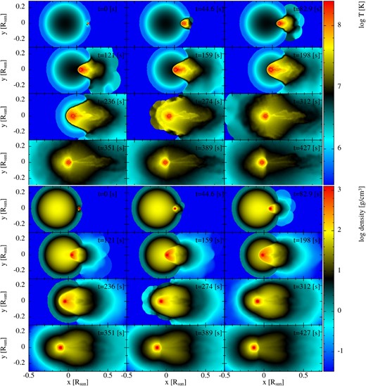
The WD is placed on the surface of the MS star at |$t = 0$| s, thus tidal distortion effects are neglected (see Appendix C for discussion about its potential impact). As the WD starts to penetrate the outer envelope of the MS star, the MS star material is accelerated towards the WD. This material then flows around the WD, is advected downstream behind the WD, and is then ejected with velocities around |$\sim\!\! 1\!\!-\!\!2 \times 10^{3}$| km s|$^{-1}$|. A high-pressure and high-density region is created in front of the WD as it moves through the MS star, which steepens into a shock around |$t=100$| s.
Once the shock is formed, we see MS star material forced to flow along the shock where it is eventually pulled back towards the region behind the WD by gravity. The motion creates two vortices at |$t \approx 504$| s (shown by large black arrows in Fig. 1), one above and one below the WD, which results in a flow around the WD surface from the back of the WD to the front. There is also MS star material that flows along the shock, falls back towards the WD, but does not form part of the vortex. This material falls into the wake of the WD and a hot, low-density turbulent flow is formed that is advected downstream as can be seen in Fig. 2 (e.g. at |$t \sim$| 638–1147 s). The shocked material reaches densities and temperatures of |$\sim$|200 g cm|$^{-3}$| and 0.1–|$1 \times 10^{8}$| K, respectively. The MS star material in the vicinity of the WD becomes very dense (|$\rho _{\rm max} \sim 230$| g cm|$^{-3}$|) and hot (|$T_{\rm max} \sim 1.5 \times 10^{8}$| K) as the WD moves through the density gradient towards the centre of the MS star. These values are maintained throughout the crossing time of the WD (|$\sim\!\! 700$| s, normalized time |$\sim\!\! 1$|).
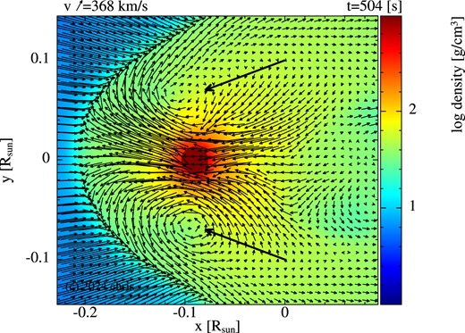
A density cross-section in the plane of the collision axis (xy-plane) with velocity vectors indicating the increased velocity of MS star material in front and around the WD as it travels through the centre of the MS star. The WD is moving from right to left.
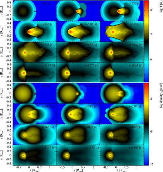
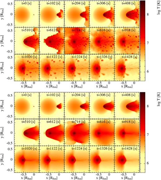
Snapshots of the time evolution of temperature (top) and density (bottom) cross-sections in the xy-plane for the |$q=1$| case.
As the WD reaches the denser parts of the MS star, it loses kinetic energy, converting it into heat that is transferred to the surrounding material. This is due to both hydrodynamic and gravitational drag acting on the WD as it moves into denser regions. At |$t \sim \, 400$| s, the WD reaches the central region of the MS star, having lost almost all of its kinetic energy (see Fig. 3). In Fig. 3, normalized time, as referred to in many of the figures in this work, is the physical time of the simulation divided by this crossing time; thus, the WD reaches the central regions at a normalized time of |$\sim\!\! 0.53$|, which corresponds to where the WD starts to lose velocity in Fig. 3. The distance between the shock and the WD increases at this point (see both the temperature and density in Fig. 2), due to the transfer of the WD’s kinetic energy to the surrounding material and the shock now moving through a negative density gradient. This can be seen in Fig. 1, where the velocity of the material around and ahead of the WD increases in the direction of motion of the WD. The vortices mentioned above start to drift away from the WD as the shock that contained them is accelerating away from the WD and will eventually dissipate. The apex of the shock along the collision axis becomes slightly elongated due to momentum transfer and accelerating first through the negative density gradient. The shock then travels through the remaining envelope of the MS star, until it eventually breaks through the outer envelope of the MS star where hot MS star material (|$T \sim 5 \times 10^{7}$| K) is ejected at |$t \sim \, 600$| s. As shown in Fig. 3, rapid mass-loss starts to take place around this time (normalized time |$\sim\!\! 0.85$|) as the shock breaks through the outer envelope of the MS star. This hot plasma produced by the crossing of the shock through the stellar surface may result in a soft X-ray/ultraviolet flash, as suggested by Rozyczka et al. (1989). In Tables 2 and 3, we show the abundances of various elements, element ratios, and isotopic ratios for the three cases presented in this paper. We note that these values are rough estimates given the uncertainties and simplifications in our nuclear reaction network. In Table 3, we give the ratio of the final abundances of the stable isotopes within our network relative to their solar values. These isotopes may be detected in follow-up observations since they are stable (long-lived). The total mass of each species that is bound and unbound to the WD at the end of the simulation is given in the last two columns for each mass ratio.
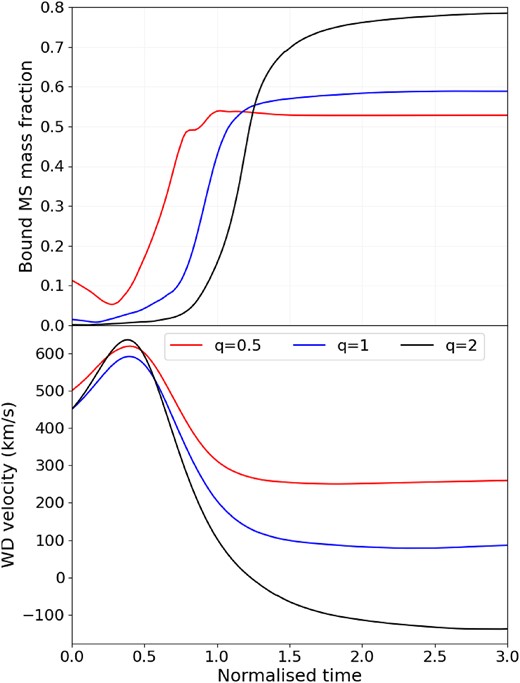
Fraction of MS material bound to the WD (top) and velocity of the WD (bottom) as a function of normalized time for |$q=0.5$| (red), |$q=1$| (blue), and |$q=2$| (black).
Elemental abundances, ratios, and isotopic ratios for different qs after two normalized times have passed.
| Ratio | q = 0.5 | q = 1 | q = 2 | Solar |
|---|---|---|---|---|
| C | |$2.33\times 10^{-3}$| | |$2.99 \times 10^{-3}$| | |$3.02 \times 10^{-3}$| | |$3.03 \times 10^{-3}$| |
| N | |$1.88 \times 10^{-3}$| | |$1.13 \times 10^{-3}$| | |$1.16 \times 10^{-3}$| | |$1.10 \times 10^{-3}$| |
| O | |$8.57 \times 10^{-3}$| | |$9.53 \times 10^{-3}$| | |$9.60 \times 10^{-3}$| | |$9.6 \times 10^{-3}$| |
| N/C | 0.69 | 0.461 | 0.391 | 0.36 |
| C/O | 0.257 | 0.303 | 0.314 | 0.319 |
| N/O | 0.178 | 0.140 | 0.123 | 0.115 |
| |$^{12}$|C/|$^{13}$|C | 42 | 51.49 | 60.0 | 90 |
| |$^{14}$|N/|$^{15}$|N | 6.62 | 19.71 | 48.79 | 440 |
| |$^{16}$|O/|$^{17}$|O | 22.11 | 73.84 | 296.1 | 2600 |
| |$^{16}$|O/|$^{18}$|O | 645 | 498.9 | 463.2 | 500 |
Nucleosynthetic yields of stable isotopes for all cases after the simulation. The first column for each q gives the ratio of the final abundance to the solar value, the second column gives the mass fraction of each species still bound to the WD, and the third column gives mass fraction of each still unbound with respect to the WD. The amount of MS star material bound to the WD is 0.16, 0.35, and 0.94 |${\rm M}_{\odot }$| for |$q=0.5, 1,\ \mathrm{ and} \ 2$|, respectively.
| q = 0.5 | q = 1 | q = 2 | |||||||
|---|---|---|---|---|---|---|---|---|---|
| Species | Final/solar | Bound | Unbound | Final/solar | Bound | Unbound | Final/solar | Bound | Unbound |
| |$^{1}$|H | 0.997 | 0.706 | 0.707 | 0.998 | 0.707 | 0.707 | 0.998 | 0.707 | 0.707 |
| |$^{4}$|He | 0.999 | 0.276 | 0.276 | 0.998 | 0.276 | 0.276 | 0.998 | 0.276 | 0.276 |
| |$^{7}$|Li | 0.026 | |$1.66 \times 10^{-12}$| | |$5.25 \times 10^{-10}$| | 0.356 | |$2.17 \times 10^{-9}$| | |$5.01 \times 10^{-9}$| | 0.644 | |$6.11 \times 10^{-9}$| | |$5.85 \times 10^{-9}$| |
| |$^{7}$|Be|$^{*}$| | |$3.87 \times 10^{-6}$| | |$2.56 \times 10^{-6}$| | |$3.60 \times 10^{-7}$| | |$1.15 \times 10^{-6}$| | |$1.04 \times 10^{-6}$| | |$1.31 \times 10^{-6}$| | |$3.94 \times 10^{-7}$| | |$2.85 \times 10^{-7}$| | |$7.29 \times 10^{-7}$| |
| |$^{8}$|B|$^{*}$| | |$1.19 \times 10^{-9}$| | |$4.47 \times 10^{-10}$| | |$6.29 \times 10^{-11}$| | |$6.91 \times 10^{-10}$| | |$1.17 \times 10^{-9}$| | |$1.35 \times 10^{-15}$| | |$2.15 \times 10^{-10}$| | |$2.85 \times 10^{-10}$| | |$5.30 \times 10^{-13}$| |
| |$^{12}$|C | 0.722 | |$1.94 \times 10^{-3}$| | |$2.49 \times 10^{-3}$| | 0.911 | |$2.73 \times 10^{-3}$| | |$2.82 \times 10^{-3}$| | 0.977 | |$2.99 \times 10^{-3}$| | |$2.93 \times 10^{-3}$| |
| |$^{13}$|C | 3.686 | |$2.13 \times 10^{-4}$| | |$4.70 \times 10^{-5}$| | 2.247 | |$1.03 \times 10^{-4}$| | |$1.18 \times 10^{-5}$| | 1.352 | |$4.81 \times 10^{-5}$| | |$5.40 \times 10^{-5}$| |
| |$^{14}$|N | 1.382 | |$1.80 \times 10^{-3}$| | |$1.23 \times 10^{-3}$| | 1.110 | |$1.27\times 10^{-3}$| | |$1.18 \times 10^{-3}$| | 1.023 | |$1.13 \times 10^{-3}$| | |$1.14 \times 10^{-3}$| |
| |$^{15}$|N | 80.01 | |$4.93 \times 10^{-4}$| | |$1.89 \times 10^{-4}$| | 17.02 | |$7.33 \times 10^{-5}$| | |$7.64 \times 10^{-5}$| | 5.309 | |$1.89 \times 10^{-5}$| | |$3.65 \times 10^{-5}$| |
| |$^{16}$|O | 0.819 | |$7.36 \times 10^{-3}$| | |$8.49 \times 10^{-3}$| | 0.964 | |$9.25 \times 10^{-3}$| | |$9.33 \times 10^{-3}$| | 0.992 | |$9.56 \times 10^{-3}$| | |$9.52 \times 10^{-3}$| |
| |$^{17}$|O | 171.1 | |$9.41 \times 10^{-4}$| | |$3.59 \times 10^{-4}$| | 39.52 | |$1.63 \times 10^{-4}$| | |$1.42 \times 10^{-4}$| | 8.267 | |$2.80 \times 10^{-5}$| | |$4.51 \times 10^{-5}$| |
| |$^{18}$|O | 0.541 | |$9.30 \times 10^{-6}$| | |$1.46 \times 10^{-5}$| | 0.820 | |$1.72 \times 10^{-5}$| | |$1.87 \times 10^{-5}$| | 0.948 | |$2.10 \times 10^{-5}$| | |$1.95 \times 10^{-6}$| |
| |$^{19}$|F | 0.658 | |$2.08 \times 10^{-7}$| | |$3.35 \times 10^{-7}$| | 0.903 | |$3.61 \times 10^{-7}$| | |$3.76 \times 10^{-7}$| | 0.976 | |$3.98 \times 10^{-7}$| | |$3.93 \times 10^{-7}$| |
| |$^{20}$|Ne | 0.945 | |$1.54 \times 10^{-3}$| | |$1.54 \times 10^{-3}$| | 0.992 | |$1.61 \times 10^{-3}$| | |$1.61 \times 10^{-3}$| | 0.997 | |$1.62 \times 10^{-3}$| | |$1.62 \times 10^{-3}$| |
Note. |$^{*}$|These isotopes show the final mass fraction and not the ratio to solar abundance in the first column of each q.
We can see from Table 3 that the H and He isotopes remain unchanged, the time-scale of the collision is too short for any considerable hydrogen fusion, and the temperatures are not high enough to start triple-alpha reactions in which |$^{4}$|He would be consumed. There is a significant depletion of |$^{7}$|Li due to it being converted to |$^{7}$|Be and |$^{8}$|B via the |$^{7}$|Li(|$p, \gamma)^{8}$|B reaction. However, after |$\sim$|53.3 d (the half-life of |$^{7}$|Be), given that the ejecta is cool enough, most of the |$^{7}$|Be in the ejecta will be transformed into |$^{7}$|Li by electron captures, possibly resulting in an overabundance of |$^{7}$|Li in the ejecta. The MS star material bound to the WD, however, will remain lithium deficient over a longer time-scale and the stellar remnant may show a deficiency of |$^{7}$|Li as a result. We note from Table 3 that during the first hour of the interaction an overabundance of |$^{13}$|C, |$^{15}$|N, and |$^{17}$|O is produced, which is evidence of incomplete CNO burning. Fig. 4 shows how the ratios in Table 2 change during the simulation; we see that significant burning happens in the central regions of the MS star where we find the densest, hottest MS star material.
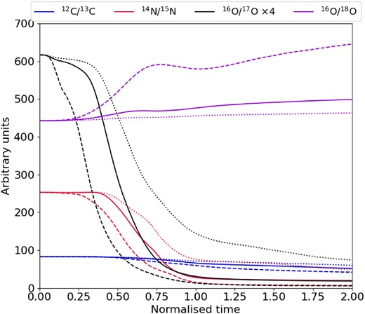
Ratios of different stable isotopes as a function of normalized time. The solid lines show the ratios for |$q=1$|, dashed lines represent |$q=0.5$|, and the dotted lines are for |$q=2$| case.
During the entire simulation (|$\sim$|36 min), |$\sim\!\! 1.21 \times 10^{48}$| erg is generated via nuclear reactions. Of this, only |$\sim$||$5 \times 10^{47}$| erg is released during the crossing time (|$\sim$|12 min) of the WD through the MS star (Fig. 5). The ratio of the MS star binding energy (|$\sim\!\! 1.4\times 10^{48}$| erg) to energy produced via nuclear reactions during the crossing time, |$\beta \equiv E_{\rm nuc}/ E_{\rm bind}$|, is |$\sim\!\! 0.14$| when the WD reaches the centre of the MS star, and is |$\beta \sim 0.3$| when the WD has crossed through the MS star outer envelope. Thus, although nuclear reactions generate a significant amount of energy, that energy is not sufficient to disrupt the MS star in the equal-mass (|$q=1$|) scenario. The nuclear energy generated in our simulations is slightly lower than the estimates derived by Shara & Regev (1986) of |$\sim\!\! 1.69 \times 10^{48}$| erg within the first 20 min of the collision, which was obtained using a power-law approximation to represent the energy release via the hot CNO cycles.
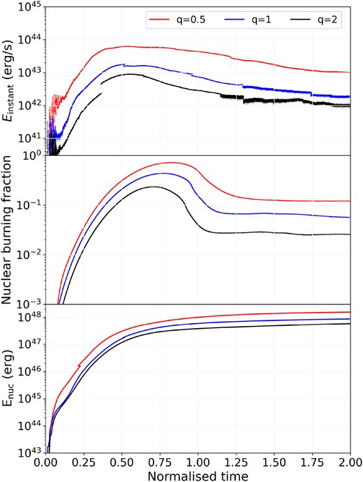
Comparison of instantaneous energy release, |$E_{\rm instant}$| (top), fraction of MS star material undergoing nuclear burning (middle), and cumulative energy release from the nuclear network (|$E_{\rm nuc}$|, bottom) as a function of normalized time for |$q=0.5$| (red), |$q=1$| (blue), and |$q=2$| (black).
However, the energy released via the nuclear reactions will have a considerable effect on the bound mass around the WD and how the remnant evolves dynamically and chemically. Since the material bound to the WD is dense and hot, nuclear reactions continue to generate a significant amount of energy (see Fig. 5). It is also evident from this figure that a significant amount of MS star material is hot enough to undergo CNO and hot CNO-cycle burning throughout the simulation. The further evolution (over several hours) of the stellar remnant is discussed in Section 3.4. After 36 min, around 45 per cent (0.27 |${\rm M}_{\odot }$|) of the MS star material is still bound to the WD. Our mass-loss estimate, although 5 per cent greater, is within the uncertainties in broad agreement with that predicted by Rozyczka et al. (1989) and Ruffert (1993). Our maximum temperature and density estimates are as much as two times higher than the |$7.8 \times 10^{7}$| K and 100 g cm|$^{-3}$| estimate found by Rozyczka et al. (1989). We attribute this to the higher resolution of our simulation in the vicinity of the WD, and the implementation of a finite radius for the WD, as was also found by Ruffert (1993).
3.2 Mass ratio: q = 2
The collision between a |$1.2\ {\rm M}_{\odot }$| MS star and a |$0.6\ {\rm M}_{\odot }$| WD (model q2_34iso) is shown in Fig. 6. The impact velocity is again 900 km s|$^{-1}$| and as with the collision above, the simulation begins with the WD on the surface of the MS star. The dynamics of the interaction between the WD and MS star material during the crossing time are similar to the |$q=1$| case. As the WD moves through the steep density gradient towards the centre of the MS star (|$t \sim 800$| s), it starts to lose kinetic energy, converting it into heat that is transferred into surrounding material (see Fig. 3, normalized time |$\sim\!\! 0.6$|).

Snapshots of the time evolution of temperature (top) and density (bottom) cross-sections in the xy-plane for the |$q=2$| case.
The amount of energy converted is less than that in the |$q=1$| case, and it gets transferred less rapidly since the density gradient of the more massive MS star here is less steep than that of the |$0.6\ {\rm M}_{\odot }$| MS star in |$q=1$|. The pronounced elongation of the shock front along the collision axis that was due to the large energy injection and steep, negative density gradient in the lower mass ratio case is also absent (see Fig. 6, |$t=1020$| s panel). The MS star material around the WD reaches densities and temperatures of |$\rho _{\rm \max } \sim$| 90 g cm|$^{-3}$| and |$T_{\rm max} \sim 1 \times 10^{8}$| K, respectively, in the central region of the MS star where we expect the largest amount of MS star material to undergo CNO and hot CNO-cycle burning and to release energy more rapidly. This can be seen in the top and middle panels of Fig. 5, where the peak nuclear burning fraction and instantaneous nuclear energy release occurs at normalized time of |$\sim\!\! 0.66$|, which corresponds to the time where the WD reaches the centre of the MS star. The shock then accelerates down the negative pressure gradient and breaks through the back-end of the MS star after |$t\sim 1250$| s (normalized time|$\sim\!\! 1$|).
The amount of nuclear energy released during the crossing time (|$\sim$|22 min) is |$E_{\rm nuc} \sim 2.96 \times 10^{47}$| erg, just under half that generated in the |$q=1$| case, but over double the time. This is due to the slightly lower maximum temperatures, and much lower densities around the WD in this case, and demonstrates the sensitivity of the nuclear reactions to the hydrodynamic conditions. Moreover, a smaller fraction of MS star gas reaches high enough temperatures to undergo hot CNO-cycle burning (Fig. 5, middle panel). Given the high temperature dependence of CNO cycles, a slight decrease in maximum temperature results in less nuclear energy released, as found in this simulation.
Comparing the total nuclear energy generated to the binding energy of the MS star (|$\sim\!\! 3.3\times 10^{48}$| erg) at the centre and outer envelope, we find |$\beta \sim 0.03$| and |$\beta \sim 0.07$|, respectively. Thus, for collisions between stars with larger mass ratios, nuclear reactions contribute less to the disruption of the MS star, and are primarily necessary for estimating nucleosynthetic yields for the remnant. The more massive MS star shifts the system’s COM closer to the COM of the disrupted MS star gas. This causes the WD to lose enough kinetic energy during its crossing time that it stops shortly after breaking through the outer envelope of the MS star and falls back towards the COM of the disrupted gas, located approximately around |$x = 0.65$| |$\mathrm{R}_{\odot }$| (Fig. 6, |$t=1403$| s panel).
The WD’s kinetic energy at the start of the interaction is of the order of |$E_{\rm kin} \sim 10^{48}$| erg. To estimate the hydrodynamic drag the WD experiences, we assume that it moves through MS star gas of average density |$\rho _{\rm ave}\, \sim$| 100 g cm|$^{-3}$|, with a relative velocity to the surrounding MS star material of |$V_{\rm rel} \sim$| 1000 km s|$^{-1}$| over a distance |$D \sim \, 2R_{\rm MS}$|. The order-of-magnitude approximation for the hydrodynamic drag is then |$E_{\rm hydro,drag} = \pi \, R_{\rm WD}^{2} \, \rho _{\rm ave} \, V_{\rm rel}^{2} \, D \sim 2 \times 10^{47}$| erg. The dynamical friction or gravitational drag the WD experiences due to the presence of the doubly massive MS star can be approximated (using similar assumptions as for hydrodynamic drag) by |$E_{\rm grav, drag} = G^{2}\, M_{\rm WD}^{2} \, \rho _{\rm ave} \, D \, /\, V_{\rm rel}^{2} \, \sim 3 \times 10^{47}$| erg. Thus, we can see from the estimates that the loss of WD kinetic energy is due to the combination of both hydrodynamic and gravitational drag on the WD as it passes through the more massive MS star.
As the WD moves through the disrupted MS star material, a different shock forms and similar flow patterns, i.e. two vortices, start to appear on both sides of the WD. This new shock has a lower speed and wider opening angle than the initial shock, which formed as the WD first entered the MS star. After 1 h (normalized time |$\sim\!\! 3$|), |$\sim\!\! 80{{\ \rm per\, cent}}$|, i.e. |$\sim\!\! 0.96\ {\rm M}_{\odot }$|, of the MS star material is bound to the WD, which is now moving at 100 km s|$^{-1}$| in the opposite direction to that in which it started its interaction.
3.3 Mass ratio: q = 0.5
The collision between a |$0.3\ {\rm M}_{\odot }$| MS star and a |$0.6\ {\rm M}_{\odot }$| WD (model q05_34iso) is shown in Fig. 7. The impact velocity is 1000 km s|$^{-1}$| and the WD is placed on the MS star surface at |$t = 0$| s. The WD accelerates through the outer envelope of the MS star and moves through a steep density gradient, which slowly causes it to lose kinetic energy (|$\sim\!\! t=200$| s). When the WD reaches the core of the MS star, the MS star material around the WD reaches densities and temperatures of |$\rho _{\rm max} \sim 400$| g cm|$^{-3}$| and |$T_{\rm max} \sim 2 \times 10^{8}$| K, respectively. Once the shock moves past the densest region, it starts accelerating down the negative density gradient until it breaks through the outer envelope of the MS star. The crossing time of the WD is |$\sim\!\! 300$| s (normalized time |$\sim\!\! 1$|). The amount of nuclear energy released during the crossing time is |$E_{\rm nuc} \sim 2\times 10^{47}$| erg.
Snapshots of the time evolution of temperature (top) and density (bottom) cross-sections in the xy-plane for the |$q=0.5$| case.
The higher temperature and densities reached result in more rapid burning, which can be seen in Table 3 and the top panel of Fig. 5, where the deviation from the solar abundances is larger compared to the higher mass ratio cases. After 25 min, the WD is moving in its original direction at |$\sim\!\! 250$| km s|$^{-1}$|, with 53 per cent, i.e. |$0.14\ {\rm M}_{\odot }$|, of MS star material bound to it (see Fig. 3). In this interaction, we estimate the ratio of nuclear energy to MS star binding energy (|$\sim\!\! 6.8\times 10^{47}$| erg) to be |$\beta \sim 0.55$| when the WD is at the centre of the MS star, and |$\beta \sim 1$| at the crossing time.
Overall, the role of nuclear energy release becomes more important with decreasing mass ratio. For the larger mass ratios, nuclear reactions are less important with regard to the overall dynamical outcome, and rather it is dominated by the shock that moves through the MS star. As shown in Fig. 3, the WD velocity changes less during the crossing time for lower mass ratios. Physically, this can be explained by the mass of the MS star and its gravitational effect on the WD. For the |$q=2$| case, the MS star is twice as massive as the WD; thus, its gravitational effect will be larger on the WD (decelerating and accelerating it), and thus we see larger changes in the WD velocity in this case. Conversely, in the |$q=0.5$| case, the MS star (with half the mass of the WD) has little effect on the massive WD. Furthermore, we see from Table 4 and Fig. 5 that the amount of, and rate at which, nuclear energy is produced is larger for lower stellar mass ratios. The increased nuclear energy generation on moving to smaller mass ratios can be ascribed to the higher impact velocities and the denser, hotter cores of lower mass MS stars (for |$n=1.5$| polytropes), which due to the strong temperature dependence of the CNO cycles significantly increases the energy generated via these cycles. Fig. 4 compares the evolution of |$^{12}$|C/|$^{13}$|C, |$^{14}$|N/|$^{15}$|N, |$^{16}$|O/|$^{17}$|O, and |$^{16}$|O/|$^{18}$|O for the different mass ratio scenarios; we see that the |$q=0.5$| case (dashed lines) differs the most, having undergone the most extensive nuclear burning during the collision. Conversely, we see for |$q=2$| that the burning is less significant as explained in Section 3.2.
Maximum temperature (T|$_{\rm max}$|), density (|$\rho _{\rm max}$|), pressure (|$P_{\rm max}$|), and peak energy generation rate (|$E_{\rm instant, max}$|) reached for different mass ratios.
| |$q=0.5$| | |$q=1$| | |$q=2$| | |
|---|---|---|---|
| T|$_{\rm max}$| (|$\times 10^{8}$| K) | 1.5 | 1.4 | 1 |
| |$\rho _{\rm max}$| (g cm|$^{-3}$|) | 440 | 230 | 90 |
| |$P_{\rm max}$| (|$\times 10^{19}$| g cm|$^{-1}$| s|$^{-2}$|) | 1.6 | 0.65 | 0.5 |
| |$E_{\rm instant, max}$| (|$\times 10^{43}$| erg s|$^{-1}$|) | 5 | 2 | 0.9 |
3.4 Longer time-scale investigation
To gain insight into the longer term evolution of the stellar remnant, we ran the |$q=1$| case, but at lower resolution (model q1_34iso_50k) with |$N = 5 \times 10^{4}$| particles each for the MS star and WD. The early evolution of the interaction is similar to the higher resolution run; so, we here focus primarily on what happens beyond the crossing time until 4 h post-initial contact and interaction.
After |$\sim$|4 h, approximately 60 per cent of the MS star material remains bound to the WD. The density and temperature profiles of this material (which extends out to a radius of |$5\ \mathrm{R}_{\odot }$|, see Fig. 8) are shown in Fig. 9. The bound material is still hot and dense with temperatures and densities as |$T > 1 \times 10^6$| K and |$\rho > 10^{-2}$| g cm|$^{-3}$|, respectively. Thus, it should eventually begin burning hydrogen and helium (Shara & Regev 1986; Rozyczka et al. 1989) in shells and expand into a red giant. The remnant is moving at 100 km s|$^{-1}$|. Depending on the environment in which the collision takes place, if the velocity of the remnant (that might resemble a giant) is higher than the dispersion velocity of other giants in the local environment, this could be an observational property that leads to identifying stars that formed via direct dynamical interaction.
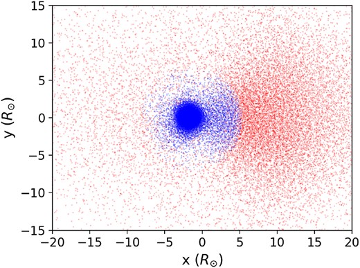
Projection of particle positions on to the xy-plane after |$\sim$|4 h for model q1_34iso_50k. The blue and red particles represent the bound and unbound material relative to the WD, respectively.
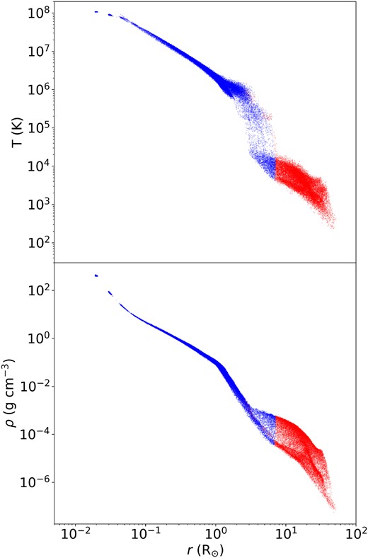
Temperature (top) and density (bottom) profiles of the MS star material |$\sim$|4 h post-collision for model q1_34iso_50k. The blue and red particles represent the bound and unbound material relative to the WD, respectively.
3.5 Observational predictions
Following the argument in Michaely & Shara (2021), if we assume that the disrupted material escapes with a velocity of |$v_{\rm esc} \sim \, 10^{3}$| km s|$^{-1}$|, and expands adiabatically, it will take about |$t \approx 10^{6}\!\!-\!\!10^{8}$| s to become optically thin. Combining this time with the energy released via nuclear reactions, the estimated bolometric luminosity for these head-on collisions in GC environments is
This is an upper limit for collisions in these environments – off-centre collisions will be less energetic and disruptive, and will thus yield lower peak luminosity estimates.
For the head-on collisions in this work, a large fraction (|$\sim\!\! 0.5$|) of the MS star material is still bound to the WD post-interaction. As seen in the longer time-scale simulation (model q1_34iso_50k, Section 3.4), at least for the |$q=1$| case the bound material is slowly expanding and slowly developing a density profile that may over a longer period of time resemble that of a red giant. Isotopic ratios of C, N, and O (see Fig. 4) in follow-up spectroscopic observations may be good indicators of such post-collision systems. An overabundance of |$^{7}$|Li is also expected in the ejecta of the collisions after sufficient time has passed for |$^{7}$|Be to transform into |$^{7}$|Li. Although the outburst luminosities of these collisions are similar to those of classical novae, there are a few properties that can be used to distinguish between them: spectroscopically, classical novae show similar overabundances of |$^{13}$|C, |$^{15}$|N, and |$^{17}$|O relative to solar values (José, Hernanz & Iliadis 2006; Das 2021); however, the production of elements heavier than neon is not expected during the collision; and the amount of material ejected from the collisions in this work is |$\sim\!\! 50{{\ \rm per\, cent}}$| of the original MS star (|$\sim\!\! 10^{-1} \ {\rm M}_{\odot }$|), which is much larger than classical nova ejecta masses (|$\sim$||$1\!\!-\!\!10 \times 10^{-5} \ {\rm M}_{\odot }$|). The stellar remnant (WD + bound MS star material) itself will continue to undergo nuclear reactions, and the effect on the structure and evolution of the remnant will be studied in future work.
3.6 Limitations of current implementation
As mentioned in Section 2.4, capturing the large density contrast between the WD and MS star particles is challenging in SPH, and this leads to an artificial ‘gap’ between the stars over which there is a very steep temperature and pressure gradient. Consequently, the WD particles do not ‘see’ the MS star particles. Since the hydrodynamic quantities in SPH are determined by summation over a finite number of nearest neighbours, the WD particles that are much more closely packed find neighbours within the WD; the smoothing lengths of WD particles do not increase sufficiently to include MS star particles. This in essence makes the WD a ‘hard sphere’. Thus, it is not possible to realistically simulate the physical processes that may occur on the surface of the WD, e.g. accretion. The estimated maximum accretion rate on to the WD is derived from the Eddington luminosity: for a |$0.6\ {\rm M}_{\odot }$| WD, this is
where |$M_{\rm acc}$| is the mass of the accretor (in our case the WD), |$m_{\rm p}$| is proton mass, and |$\sigma _{\rm T}$| is the Thompson cross-section. Setting this value equal to the accretion luminosity and solving for the accretion rate,
Assuming this rate, the WD would at most accrete about |$10^{-8}\ {\rm M}_{\odot }$| within the first 3 h after penetrating the MS star, and thus even less during the crossing time through the MS star. As we are primarily focused on the energetics and nuclear reactions that take place within the MS star gas, it is not necessary to resolve the hydrodynamics at the surface of the WD since changes there are minimal on the time-scale we are simulating. Our implementation of the WD with a finite radius should be sufficient as it results in more realistic flows in the WD region, as well as generating an accurate estimation of the gravitational potential of the WD. However, the above accretion rate is still significant in terms of considering the long-term evolution of the stellar remnant. For the |$q=2$| scenario where |$\sim\!\! 80{{\ \rm per\, cent}}$| of the MS star remains bound (|$0.96\ {\rm M}_{\odot }$|), if we assume that the WD accretes all bound material in a stable manner, it will reach the Chandrasekhar limit in less than 1000 yr and result in a Type Ia supernova. If the hydrogen-rich material accumulating on the WD surface reached ignition before that, a nova explosion could be triggered. Longer term simulations with more realistic stellar profiles are needed to determine the probability of each scenario.
4 CONCLUSION
In this work, we carried out 3D hydrodynamic simulations of head-on WD–MS collisions using SPH with a 34-isotope nuclear network. We focus on investigating the impact of nuclear reactions, the energetics, and mass lost for collisions with different stellar mass ratios. We also studied the effect of various additional physics and numerical assumptions and approximations, such as tidal distortion, AC, resolution, and using different nuclear networks. Our main results are as follows:
For all mass ratios considered, the MS star is completely disrupted. However, we find that 45–65 per cent of MS star material stays bound to the WD. This bound material should on longer time-scales start burning hydrogen and helium in shells and expand into a red giant with chemically peculiar spectroscopic signatures.
Nuclear reactions in the regime of low impact velocities studied here are not the primary disruption mechanism, at least for mass ratios of |$q\ge 1$|; however, they remain crucial in understanding nucleosynthetic processes during the collision that lead to predictions of key characteristics for follow-up observations. For mass ratios smaller than |$q\sim 1$|, nuclear reactions become more significant, generating cumulative energies close to the binding energy of the MS star. We show in the |$q=0.5$| case that nuclear reactions generate energy equal to the binding energy of the |$0.3\ {\rm M}_{\odot }$| MS star (|$\sim\!\! 10^{47}$| erg) within the crossing time of the WD (|$\sim\!\! 5$| min).
Hot CNO cycles significantly increase the amount of nuclear energy generated within these collisions and are important for the prediction of isotopic signatures.
The stellar remnants of WD–MS star collisions are likely to be lithium deficient; however, after about two months (half-life of |$^{7}$|Be, i.e. 53.3 d), the ejecta will have an overabundance (compared to solar) of |$^{7}$|Li. Similarly, isotopes such as |$^{13}$|C, |$^{15}$|N, and |$^{17}$|O are also enhanced relative to solar values.
The large amount of material ejected (|$\sim\!\! 10^{-1} \ {\rm M}_{\odot }$|) from these collisions and a lack of production of elements heavier than neon during the interaction may possibly distinguish these collisions from other transients with bolometric luminosities of |$\sim\, L_{\rm bol} \simeq 10^{5}\!\!-\!\!10^{7}\ \mathrm{ L}_{\odot }$|, e.g. classical novae.
ACKNOWLEDGEMENTS
We thank the anonymous referee for the very thorough review that greatly improved this work. We thank Frank Timmes for valuable discussions regarding the nuclear networks used in our models. SSM and CJTvdM acknowledge funding from the National Research Foundation (NRF), the South African Astronomical Observatory (SAAO), and the University of Cape Town VC2030 Award. JJ acknowledges support from the Spanish MINECO grant PID2020-117252GB-I00, the E.U. FEDER funds, and the AGAUR/Generalitat de Catalunya grant SGR-386/2021. TK acknowledges funding from grant SONATA BIS no. 2018/30/E/ST9/00398 from the Polish National Science Center. The simulations were run on the MONS cluster at SAAO as well as the Lengau cluster at the Centre for High Performance Computing (CHPC). The authors acknowledge Research Computing at The University of Virginia for providing computational resources and technical support that have contributed to the results reported within this publication (https://rc.virginia.edu). All rendered figures are made using the interactive visualization tool for SPH simulations, splash (Price 2007). We thank all contributors and developers of splash. Analysis made significant use of python 3.7.4, and the associated packages numpy and matplotlib.
DATA AVAILABILITY
The data are available upon request due to the large size of the output of the simulations.
Footnotes
https://cococubed.com/code_pages/burn_hydrogen.shtml, ‘CNO cycles’.
https://cococubed.com/code_pages/burn_hydrogen.shtml, ‘PP + Hot CNO + rp breakout’.
https://cococubed.com/code_pages/burn_helium.shtml, ‘34 isotopes’.
REFERENCES
APPENDIX A: POLYTROPE SET-UP
To set up the polytropes, we use the Weighted Voronoi Tesselation Initial Configuration (wvtic) code (Arth et al. 2019), which produces glass-like particle configurations that are converged to a user-defined density profile. To demonstrate the procedure, the set-up of an |$n=1.5$| polytrope with mass of 0.6 |${\rm M}_{\odot }$| and radius of 0.01 |$\, \mathrm{R}_{\odot }$| is shown below. The simplest approach is to generate a sphere of constant density that has a relaxed, glass-like configuration. A box of size |$0.02 \times 0.02 \times 0.02$| (solar units are used for mass and length) is defined in which the code then distributes and relaxes |$N \sim 10^{6}$| particles into the desired density profile. The resulting configuration can be seen in the left panel of Fig. A1. From this particle configuration, all particles within a radius of |$0.01\ \mathrm{R}_{\odot }$| are cut out, producing a sphere with constant density (i.e. a smooth and random distribution of particles). From the original |$N = 1 \times 10^{6}$| particles contained in the cube, roughly |$N \sim 5 \times 10^{5}$| particles are in the |$0.01\ \mathrm{R}_{\odot }$| sphere.
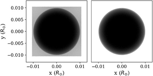
Glass-like particle configuration with constant density sphere in the centre (left), and the |$0.6\ {\rm M}_{\odot }$|, |$0.01\ \mathrm{R}_{\odot }$| constant density sphere that is cut out for relaxation (right).
Although the initial particle configuration was in a relaxed state, after cutting out the sphere, the sphere itself is not in a relaxed state. We therefore need the particles to interact again to reach a new equilibrium. To relax the sphere, we simply take the particle configuration shown in the right panel of Fig. A1 and put it in a simulation as an isolated sphere and let it evolve until the ratio of the total specific internal energy (U) over the total gravitational energy (|$\Omega$|) of the particles converges to a value close to |$U/ \Omega \sim -0.5$| (see second panel of Fig. A2). We assume equal-mass particles and set initial particle velocities to zero. We keep the specific entropy of all particles constant, due to the lack of convection zones in lower mass MS stars. The value for the polytropic constant is calculated from the standard polytropic equations to be |$K \sim 2.09 \times 10^{12}$| for an |$M = 0.6\ {\rm M}_{\odot }, R = 0.01\ \mathrm{R}_{\odot }$||$n=1.5$| polytrope. Relaxation of the polytrope that was generated with the wvtic method using |$N \sim 10^{5}$| particles had a run time of 1 week using 24 cores.
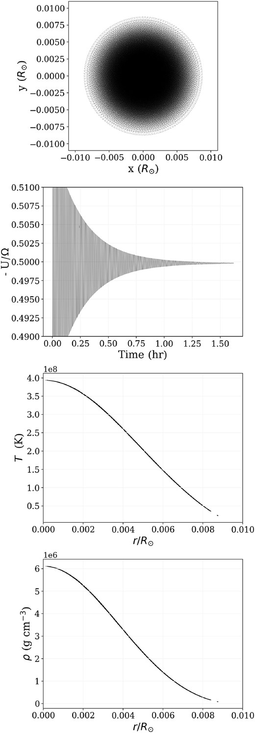
From top to bottom, the final particle configuration of a relaxed polytrope, the ratio of the thermal and gravitational energies of the polytrope during the relaxation process, the temperature profile of the relaxed polytrope, and the density profile of the relaxed polytrope.
APPENDIX B: EFFECTS OF ADDITIONAL MODULES
In order to model WD–MS star collisions, we needed to add additional modules to the default gadget-4 code. The effects of these modules are discussed in this section and depicted in Fig. B2. The default configuration of gadget-4 uses the ideal gas law as its EOS.
B1 Artificial conductivity
To reduce the effects of steep temperature and pressure gradients between the WD surface and surrounding MS star material, we implemented AC to the default gadget-4 code. In Fig. B1 using snapshots of models q1_ac and q1_default, collisions with and without AC, respectively, are compared. In the former, the shock is smoother and well defined, and the high-temperature blobs that originate near the WD surface and are advected downstream (as in Fig. B1, top) are absent. As expected, the maximum temperature decreases by almost an order of magnitude, which indicates that there are individual particles that experienced unphysical forces (see Fig. B2). The maximum density and pressure also decrease substantially and a lower amount of mass is lost during the time the WD is moving towards the centre of the MS star.
Temperature cross-sections in the xy-plane showing the time evolution of model q1_default without AC (top), and model q1_ac that includes AC (bottom).
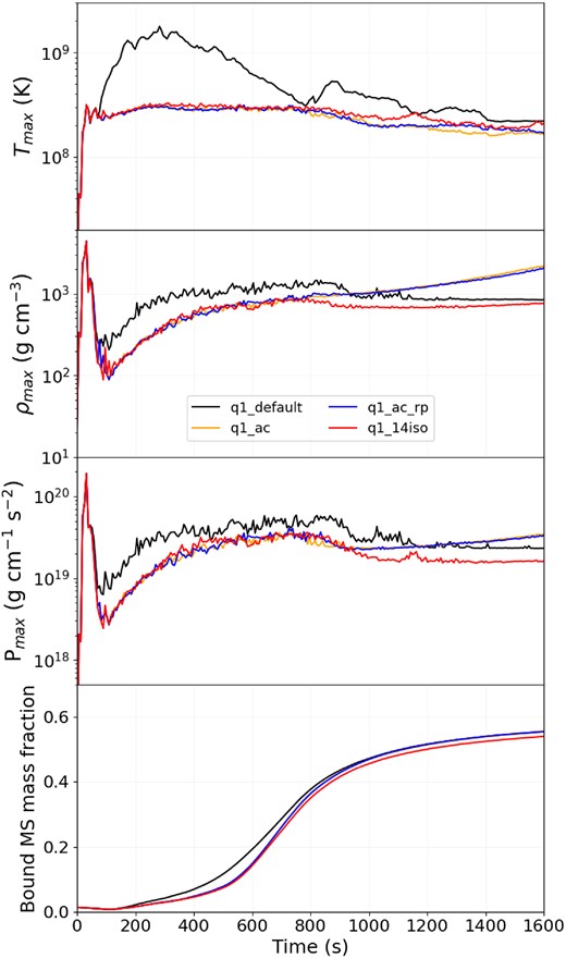
The effect that additional modules have on, from top to bottom, the maximum temperature, maximum density, maximum pressure, and fraction of bound MS star material.
B2 Radiation pressure
Fig. B2 shows that the addition of radiation pressure (model q1_ac_rp) does not have a significant impact on the hydrodynamics in the regimes we consider. This is verified by taking the maximum temperature and density reached during our simulation (|$T_{\rm max} = 1.5 \times 10^{8}$| K and |$\rho _{\rm max} = 500$| g cm|$^{-3}$|) and comparing them to the theoretical boundary between regions where ideal-gas pressure and radiation pressure dominate,
We conclude that for solar abundances, although our models are close to the radiation pressure regime, they stay in the ideal-gas regime, consequently the effect of implementing radiation pressure is small.
B3 Nuclear reactions
The implementation of a nuclear reaction network in our models is necessary to not only estimate the contribution of nuclear reactions to the dynamics and energetics during the collisions between WD and MS stars but also enables us to make predictions towards nucleosynthetic processes that might lead to unique observational signatures.
We see from comparing models q1_ac_rp and q1_14iso in Fig. B2 that there is a small effect from including a nuclear network that only contains CNO-cycle reactions, namely slightly higher maximum temperatures, slightly lower maximum densities and pressure at later times in the collision where the WD has passed through the densest parts of the MS star, and lastly we see slightly less MS star material bound to the WD. The main reason for this is the additional energy that is now being released in the region around the WD, which pushes out material, leading to lower density and pressure in the vicinity around the WD and cumulatively leads to more particles having higher total energy and becoming unbound.
We additionally compared three ‘hard-wired’ nuclear reaction networks in this work. The first is the previously mentioned 14-isotope network6 (model q1_14iso) that covers the normal CNO cycles. The second network contains 26 isotopes7 (model q1_26iso) and approximates energy generation for pp-chain, normal CNO, and hot CNO cycles, with breakout reactions also included. Finally, the largest network we considered is a 34-isotope network8 (model q1_34iso), which combines the above 26-isotope network with a 13-isotope network that uses an alpha-chain from helium to nickel.
Looking at Fig. B3, we can see an increase in maximum temperature around the time that the WD starts to reach the densest, hottest parts of the MS star (|$\sim$|300–400 s). This increase in energy leads to more significant effect in the form of even lower density, pressure, and bound mass estimates compared to the model that does not have any nuclear reactions (q1_ac_rp). Comparing these three networks (Fig. B4) shows that models that include the hot CNO cycles, i.e. the 26- and 34-isotope networks, start to generate significantly more energy as the temperatures and densities start to reach values of |$T > 1 \times 10^{8}$| K and |$\rho > 100$| g cm|$^{-3}$|, respectively (see Fig. B3, first and second panels). Thus, under these conditions, we need to include hot CNO cycles to better estimate the nuclear energy released during the collision. However, the 26- and 34-isotope networks in Fig. B4 give the same result; thus, under these conditions alpha-chain reactions are not triggered or generate negligible energy, since the temperatures and densities are not high enough. This means that the 26-isotope network is sufficient for the simulations in this work; however, given our planned future work, we decided to use the 34-isotope network as our default network.
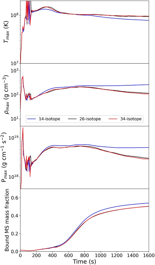
The effect of different networks on, from top to bottom, the maximum temperature, maximum density, maximum pressure, and the fraction of MS star material bound to the WD during the collision.
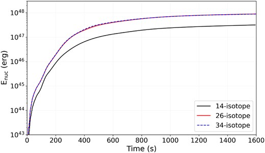
Comparison of cumulative nuclear energy release for models q1_14iso (black, solid), q1_26iso (red, solid), and q1_34iso (blue, dashed).
APPENDIX C: TIDAL DISTORTION
The effect of tidal distortion becomes more important in low-velocity collisions (Shara & Shaviv 1977, 1978; Shara & Regev 1986). To understand the effect that our initial conditions have on the hydrodynamics and energetics of the collision, we compare two simulations: one in which the stars are separated by a few stellar radii, and the other in which the WD is initially placed at the surface of the MS star. In the separated model, the centres of the stars are initially placed |$1.2 \ \mathrm{R}_{\odot }$| apart with a relative velocity of |$v_{\rm rel} \sim 600$| km s|$^{-1}$| at |$t=0$| s. The broad outcomes of the collision remain the same for both starting positions. The largest difference between the models with the two starting positions is the maximum pressure of the MS star gas that is reached during the simulation being |$\sim\!\! 30{{\ \rm per\, cent}}$| higher and a larger opening angle is produced for the shock in the model where the stars are initially separated, as shown in Fig. C1. In the separated case, the MS star material closest to the WD is distorted into a cone-like geometry and funnelled towards the WD. When the WD is placed at the surface of the MS star, the initial velocities of the MS star particles are calculated independently of the WD’s gravitational pull. Thus, it takes a few seconds for the MS star material to react to the presence of the WD when the simulation starts, and the MS star material starts to accelerate towards the WD.
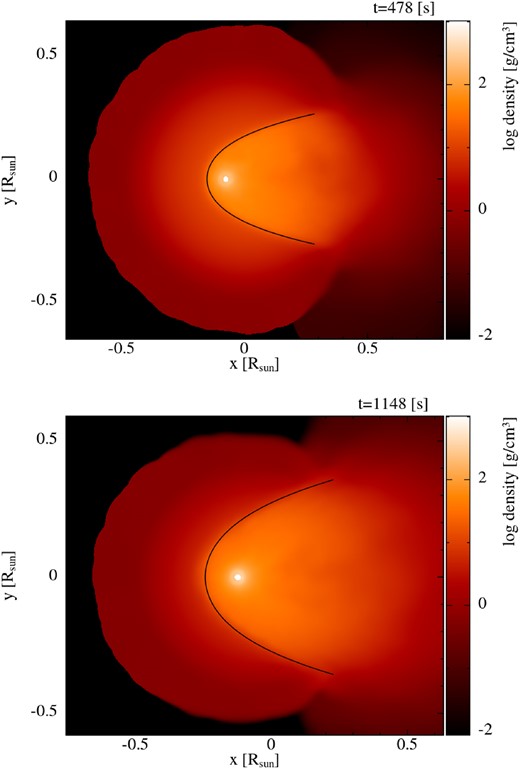
Density cross-sections in the plane of the collision axis showing the well-defined shock just before breaking through the MS star surface for the case where the WD starts on MS star surface (top), and the stars are initially separated (bottom). The WD is located in the highest density region. The black lines represent a typical bow shock structure based on the analytical solution presented in Wilkin (1996). A rough estimate is given for the shock stand-off distance |$R_0$|.
The distortion of the MS star material leads to more concentrated flow of MS star material towards and around the WD, which results in higher resolution (less variability) at early times for the hydrodynamic quantities as seen in Fig. C2. This is a result of the inherit characteristic of SPH that resolution follows mass (the number of particles) when using equal-mass particles. The funnelling also results in more material having higher kinetic energies (and thus total energies), which leads to lower bound mass estimates as seen in the top right panel of Fig. C2. The funnelling of the MS star material towards the WD causes it to reach lower maximum velocity and the WD loses kinetic energy less rapidly than when started on the surface (Fig. C2, right middle panel). The nuclear energy generation for the separated case is lower initially as the funnelling of MS star material results in less material reaching nuclear burning conditions at early times. However, the larger opening angle of the shock for the separated case leads to more MS star material being shocked to high enough temperatures to undergo nuclear burning during the collision, which leads to a higher cumulative nuclear energy estimate for the separated case after |$t\sim \, 1000$| s (see Fig. C2, right bottom panel). We thus note here that our results in this work should be seen as lower limits to the amount of energy that could be generated via nuclear reactions.
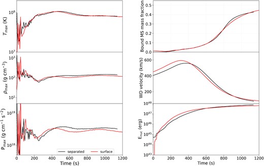
The left panels show the effect of starting position on the maximum temperature (top), maximum density (middle), and maximum pressure (bottom). The right panels show the effect on fraction of MS material that is bound to the WD (top), the WD velocity (middle), and the cumulative nuclear energy generation during the collision (bottom). The time axis for the separated case has been shifted left by 450 s. This is about the time it took the WD from its initial position to enter the MS star.
APPENDIX D: CONVERGENCE STUDY
To investigate the effect that resolution may have on the energetics and dynamics of these collisions, we varied the number of particles used for each star from |$N = 5 \times 10^{4} \ \mathrm{ to} \ N = 5 \times 10^{5}$| (i.e. models q1_34iso_50k, q1_34iso_200k, and q1_34iso). Fewer particles result in poorer shock resolution and lower estimates for the hydrodynamic quantities of interest (see Fig. D1, left panels and Fig. D2); this is a result of the smoothing lengths of particles that changes with resolution, since the number of neighbours remains fixed. When a particle’s smoothing length is increased, it effectively smooths the quantity of interest over a larger volume, leading to lower estimates. Moreover, lower resolution of the flow of MS star material in the vicinity of the WD delays the appearance of the shock and the vortices described in Section 3.1. This is due to a lack of particles in the outer envelope of the MS star; as the WD moves through denser parts of the MS star (where there are more particles, i.e. higher resolution), the flow becomes similar to that of the higher resolution models. Since the deviation between models q1_34iso_200k and q1_34iso is small, we conclude that, given the available computational resources, we get reasonable results using |$N \sim 10^5\!\!-\!\!10^6$| particles for each star. The effect of resolution on the nuclear network (Fig. D1, bottom right panel) is difficult to quantify, since it is very sensitive to the temperatures and densities that are given as initial conditions at every time-step.

The left panels show the effect of resolution on the maximum temperature (top), density (middle), and pressure (bottom) during the collision. The right panels show the effect of resolution on the bound MS mass fraction (top), WD velocity (middle), and cumulative nuclear energy release (bottom) during the collision.
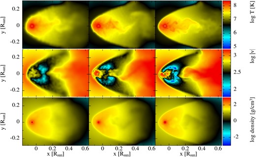
Snapshots of temperature (top row), density (middle row), and absolute velocity (bottom row) cross-sections in the xy-plane case. The left panels represent model q1_34iso_50k, the middle panels correspond to q1_34iso_200k, and the right panels show our final resolution run of model q1_34iso. All panels are for the same time (|$t=440$| s) for each model.
