


ABSTRACT
Magnetic reconnection before flux cancellation in the solar photosphere when two opposite-polarity photospheric magnetic fragments are approaching one another is usually modelled by assuming that a small so-called ‘floating current sheet’ forms about a null point or separator that is situated in the overlying atmosphere. Here, instead we consider the reconnection that is initiated as soon as the fragments become close enough that their magnetic fields interact. The resulting current sheet, which we term a ‘fin sheet’ extends up from the null point or separator that is initially located in the solar surface. We develop here non-linear analyses for finite-length models of both fin and floating current sheets that extend the previous models that were limited to short floating current sheets. These enable the length of the current sheet and the rate of heating to be calculated in both cases as functions of the separation distance of the sources and the reconnection rate. Usually, the fin current sheet liberates more energy than a floating current sheet.
1 INTRODUCTION
Pontin et al. (2024) have proposed that magnetic reconnection driven by photospheric flux cancellation may contribute substantially to the heating of the solar corona and the acceleration of the solar wind. Such reconnection has for long been associated with a range of dynamic events in the solar atmosphere, such as X-ray right points (Martin, Livi & Wang 1985; Parnell, Priest & Titov 1994; Priest, Parnell & Martin 1994; Parnell & Priest 1995; Archontis & Hansteen 2014), X-ray jets (Shibata et al. 1992; Shimojo et al. 2007), UV bursts in active regions (Peter & Dwivedi 2014), and transition-region explosive events (Brueckner & Bartoe 1983; Innes et al. 1997). Flux cancellation was thought before 2010 to take place mainly near the boundaries of supergranules, since that was where most of the photospheric magnetic flux observed at that time was concentrated (e.g. Schrijver et al. 1997; Priest 2014).
However, ground-breaking observations from the SUNRISE balloon mission (Lagg et al. 2010; Solanki et al. 2011, 2017; Smitha et al. 2017) have transformed our view by showing that flux cancellation is very much more common than previously thought and often occurs around granules. This has been shown to imply that flux cancellation may be a viable mechanism for heating the chromosphere and corona (Priest, Chitta & Syntelis 2018), and a series of models for the process has been developed (Syntelis, Priest & Chitta 2019; Syntelis & Priest 2020; Priest & Syntelis 2021; Syntelis & Priest 2021). In addition, clear examples of impulsively enhanced emission triggered by flux cancellation have been discovered, including in coronal loops (Tiwari et al. 2014; Huang et al. 2018), in association with UV bursts and bidirectional jets (Chitta et al. 2017) and campfires (Panesar et al. 2021), in the cores of active regions (Chitta, Peter & Solanki 2018; Chitta et al. 2020), and either between bipolar footpoints or between such a footpoint and an opposite-polarity photospheric magnetic fragment (Kahil et al. 2022).
In response to slow motions of the photospheric footpoints of coronal magnetic fields on time-scales longer than the Alfvén travel time, the magnetic field evolves through a series of magnetohydrostatic equilibria. If the plasma pressure is much smaller than the magnetic pressure and the height of the structure is less than the gravitational scale-height, those equilibria will be force-free in nature, and, if the electric currents are small, they will be close to potential magnetic fields. When the equilibria are topologically complex, in the sense that they possess null points or separator field-lines, then current sheets can form around such nulls or separators and magnetic reconnection can take place at them. Current sheets can also form in topologically simple but geometrically complex configurations where nulls and separators are absent but quasi-nulls or quasi-separators are present (e.g., Pontin & Priest 2022, and references therein).
There are many ways in which current sheets can appear and evolve, as described in Priest (2014). Several techniques have been employed for modelling current sheets, each of which has pros and cons (Priest 2014). For modelling the appearance and slow evolution of current sheets in two dimensions, an invaluable and elegant technique is to use complex variable theory, as first proposed by Green (1965) and Tur & Priest (1976). Modelling them in three dimensions is much more difficult, since complex variable theory is no longer valid, but a method has been developed by Priest & Syntelis (2021) for an axisymmetric three-dimensional sheet by treating the sheet as a series of current rings (see also Longcope 1996; Longcope & Cowley 1996). For non-axisymmetric fields or to describe the time-dependent fragmentation of sheets into plasmoids or flux ropes, it is generally necessary instead to use computational MHD modelling. In this paper, on grounds of simplicity and ease of determination of the response to varying the reconnection rate or the footpoint locations, we model current sheets as two-dimensional structures in an ambient potential field.
In general, several types of model may be constructed that complement one another and give different insights about the basic physics of complex solar phenomena. On the one hand, it is possible to develop complex three-dimensional computational models that include as much realistic physics as possible. These can produce images or spectra that may be compared with detailed observations and have led to great advances in interpreting the observations. However, they are often extremely difficult to understand and are unable fully to ‘simulate’ the observations, since there is always some physics that is omitted and they cannot achieve the spatial resolution that is necessary for a full understanding. In addition, they can be run for only a few specific ranges of parameters and for limited time, due to computational constraints. Here, we adopt an alternative philosophy of constructing much simpler, largely analytical models, in which one can easily see the effects of a wide range of parameters. They use in-depth physical understanding to focus on key physical processes (here magnetohydrodynamic) while omitting others, but they are also able to produce key advances in understanding in order to interpret observations and to guide future computational experiments.
When two photospheric magnetic flux patches of opposite polarity approach one another, reconnection may be initiated at a current sheet between them. Previous modelling has assumed the current sheet forms about a null point or separator that is situated above the solar surface, typically in the corona, so that the current sheet is also detached from the surface, a situation that we refer to as a ‘floating’ current sheet. However, there is significant evidence that the reconnection may often occur lower in the atmosphere. Incidents of transient Ca ii H brightening observed by Hinode (Park & Chae 2012) suggest that reconnection associated with flux cancellation may be happening in the chromosphere or even in the photosphere (Litvinenko 2015). Nelson et al. (2013) present both observations and simulations of Ellerman Bombs initiated when flux cancellation drives magnetic reconnection at chromospheric heights. Shelyag et al. (2018) analysed simulations of magnetoconvection, identifying numerous discrete flux cancellation events in which the associated magnetic reconnection occurred in the photospheric layer in a so-called flux pile-up regime.
We here consider an alternative scenario to that of a floating current sheet, in which the current sheet grows up from the photosphere as the flux patches approach, and we call this a ‘fin’ current sheet due to its resemblance to the dorsal fin of a sea mammal (Section 2). Related ideas were considered briefly by Low & Wolfson (1988) and Low (1992). Such initially low-lying sheets may be important when energy is released low in the atmosphere, as, for example in Ellerman bombs in the low chromosphere (Rouppe van der Voort, Rutten & Vissers 2016; Hansteen et al. 2017). In addition, we generalize the previous modelling of a floating current sheet by dropping the previous assumption that the current sheet be ‘small’ in the sense that its vertical dimension is much smaller than the typical distance between flux sources (see Section 3).
Both floating and fin current sheets are likely to be important in the solar atmosphere, but their presence depends on the nature of both the magnetic topology and the motion of the phospheric magnetic fragments which can be regarded as acting as sources for coronal magnetic fields. If the topology is relatively simple and one starts with two isolated magnetic fragments that are not connected magnetically, then, as they approach one another, their magnetic fields will come into contact and a fin current sheet will naturally form. On the other hand, if the flux sources are initially connected magnetically and they start to move towards one another, then their motion will drive the formation of a floating current sheet along the separator or around the null point that was initially present. Considering a region whose topology is complex with null points or separators being present, the motion of photospheric footpoints will naturally form floating current sheets.
The paper is organized as follows. In Section 2, we present a new model for reconnection at a fin current sheet. Then in Section 3, we extend previous models of a floating current sheet to a finite length sheet. Finally, in Section 4 we present a discussion, including a comparison of the energy release in the two cases.
2 FIN CURRENT SHEET MODEL
2.1 Magnetic field model
Consider a two-dimensional magnetic field (|$B_x,B_y$|) in the solar corona (represented by the half-space |$y\gt 0$|) generated by two patches of magnetic flux in the presence of a uniform background horizontal field (|$B_0\hat{\bf \boldsymbol{ x}}$|) of strength |$B_0$|. For simplicity, we model the flux patches (which represent magnetic flux that is generated in the solar interior and is threading through the solar surface into the corona) as point sources located at |$x=\pm d$| on the y-axis. We denote the half-separation of the sources by d (see Fig. 1) and consider what happens as d decreases so that the flux patches approach one another. Here, we suppose that the time-scale for approach is much longer than the Alfvén travel time, so that the approach speed is much smaller than the Alfvén speed, and the evolution is quasi-static through a series of potential fields. The potential magnetic field of the two sources plus overlying field is given by
where
are the vector positions of the point (|$x,y$|) relative to the two sources and |$\pm F$| are the strengths of the sources.
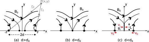
Two magnetic flux sources of flux |$\pm F$| are situated on the x-axis a distance |$2d$| apart in the presence of an overlying uniform magnetic field |$B_0$|. The distances from the sources to a point P(|$x,y$|) are given by vectors |${\bf \boldsymbol{ r}}_1$| and |${\bf \boldsymbol{ r}}_2$|. As d decreases and the sources approach one another, there are s everal stages: (a) when |$d\gt d_0=2F/(\pi B_0)$|, there are two linear null points (large dots) on the x-axis; (b) when |$d=d_0$|, the nulls combine to form a second-order null; (c) when |$d\lt d_0$|, a current sheet forms of length L at which the inflowing magnetic field is |$B_i$| and the inflow speed is |$v_i$|.
The so-called ‘flux interaction distance’ (Longcope 1998) is given by
When the sources are sufficiently far apart (|$d\gt d_0$|), the two sources are not joined by any magnetic field lines, but two magnetic null points are located between them on the x-axis (Fig. 1a). As the parameter d is decreased, the two null points approach one another, and when |$d=d_0$| they coincide at the origin (Fig. 1b). For the magnetic field described in equation (1), the x-component of the magnetic field on the y-axis is
and so, when |$d\lt d_0$|, there is a null point present on the positive y-axis, located at |$y_N=\sqrt{d_0d-d^2}$|.
Now, consider what happens as the sources approach one another, starting from |$d\gt d_0$| and ending up with |$d\lt d_0$|. In a vacuum, the magnetic field would simply pass through a series of potential fields as the two null points on the x-axis approach one another, merge, and then a null point lifts off the surface along the y-axis, while the fields continuously change their topology. However, in an ideal plasma, changes of topology are not allowed and so a current sheet would form with a length determined by magnetic flux conservation, as shown in Fig. 1c. Again, in a non-ideal plasma with, for example, finite resistivity, the reconnection rate would determine the changes in magnetic fluxes and therefore the size of the current sheet, as follows.
To represent the idealized magnetic field containing a tangential discontinuity (Fig. 1c), we follow Green (1965), Syrovatsky (1971), and Tur & Priest (1976) in using a complex-variable representation with |$z=x+iy$|. We can write the magnetic field (1) as
When |$d=d_0$| this reduces to |$B_x-iB_y = B_0z^2/(z^2-d_0^2)$|, and so for |$d\lt d_0$| we choose a magnetic field that possesses flux sources at |$z=\pm d$|, tends to |$B_x=B_0$| at infinity, includes a branch cut from |$z=iL$| to |$z=-iL$| to represent the current sheet, and reduces to the same form when |$L=0$|, namely,
For the upper half plane (|$z\ge 0$|), this has a fin current sheet [a cut in the positive complex plane (|$y\ge 0$|)] from |$y=0$| to |$y=L$|.
2.2 Fin current sheet length (L(d)) with no reconnection
The length of the current sheet (L) is expected to be a function of the source separation (|$2d$|). It is determined by a constraint that comes from conservation of the flux above the current sheet. Consider first the case where reconnection is prohibited. In that case, the flux above the current sheet must remain fixed as the flux patches approach one another. In order to calculate this flux we note that, for |$d\lt d_0$|, equation (4) gives the following expressions for the field components on the y-axis
Thus, equating the flux across the y-axis between |$y=L$| and |$y=\infty$| when |$d\lt d_0$| to the corresponding flux between |$y=0$| and |$y=\infty$| when |$d=d_0$| yields
Since both of these integrals are infinite due to the presence of the uniform component |$B_0\, \hat{\bf \boldsymbol{ x}}$| in equation (1), we subtract the integral over the uniform field out to infinity from both sides to give
where the right-hand side is simply
Next, in order to solve this equation for |$L(d)$|, we adopt a change of variable, setting |$u=y/L$|, which reduces it to
the solution of which is surprisingly simple (see Appendix A), namely,
so that the current sheet length (L) vanishes at |$d=d_0$| (as required), and it tends to |$d_0$| as d approaches zero, as shown by the black curve in Fig. 2(a).
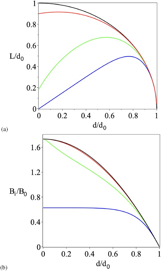
(a) Fin current sheet length |$L/d_0$| as a function of source separation |$d/d_0$| in units of the flux interaction distance (|$d_0=2F_0/(\pi B_0)$|), where |$\pm F_0$| are the fluxes of the sources and |$B_0$| is the strength of the overlying field. The sheet length in the absence of reconnection is shown in black and for |$C=\alpha /M_{A0}= 0.1$|, 1, 5 in red, green, and blue, respectively. (b) Inflow magnetic field strength |${B}_i/B_0$| for the same values of C.
2.3 Fin current sheet length with reconnection
If the plasma is not perfectly ideal, then, during the time that the flux patches approach one another, reconnection will commence in the current sheet. This will add flux above the current sheet, and the current sheet length will become smaller than when reconnection is prohibited. It is then possible to determine the sheet length (L), the inflow speed (|$v_i$|), and the inflow magnetic field (|$B_i$|) in terms of the imposed values of the flux source separation (|$2d$|), the speed of approach (|$v_0$|) of the sources, and the overlying magnetic field strength (|$B_0$|), as follows.
The magnetic flux (|$F_\mathrm{ R}$|) added above the current sheet is equal to the net flux (|$\psi$|) into the sheet, namely,
and, after defining the speed of approach of the flux sources as |$v_0=\mathop {}\!\mathrm{d}(d)/\mathop {}\!\mathrm{d}t$|, this becomes
In order to estimate the flux reconnected, we need to assume a typical inflow speed (|$v_{i}=\alpha v_{\mathrm{ A}i}$|) to the reconnection site in terms of the local Alfvén speed (|$v_{\mathrm{ A}i}$|), where |$\alpha$| depends on the nature of the reconnection and the rate at which it is being driven, as described in, e.g. Priest (2014). Thus, reconnection may be slow, with |$\alpha$| being tiny (say, |$10^{-6}$|) or it may be fast, with the maximum value of |$\alpha$| for various fast models being in the range |$0.01{\!-\!}0.1$| (e.g., Priest 2014; Cassak, Liu & Shay 2017; Pontin & Priest 2022). Then the ratio of the inflow speed to the driving speed becomes
where |$M_{\mathrm{ A}0}=v_0/v_{\mathrm{ A}0}$| and |$v_{\mathrm{ A}0}=B_0/\sqrt{\mu \rho _{i}}$| is the Alfvén speed based on the overlying magnetic field (|$B_0$|) and the density (|$\rho _{i}$|) at the inflow to the current sheet. Thus, equation (8) can be written as
where |$C=\alpha v_{\mathrm{ A}0}/v_0$| is a dimensionless constant. In this and in what follows, we for simplicity assume that |$\alpha = \mathrm{ constant}$|, but, if |$\alpha$| were non-constant, the resulting energy release would lie between the different curves associated with |$\alpha = \mathrm{ constant}$|.
Hence, to proceed in determining the length of the current sheet we modify equation (6) to include the reconnected flux to give
To estimate |$B_{i}$| we use the value at the centre of sheet, by substituting |$y=\textstyle {\frac{1}{2}}L$| into equation (5), giving
Substituting into equation (11) and evaluating the integral on the left-hand side yields
which we wish to solve for the unknown function |$L(d)$|.
To solve this equation for |$L(d)$|, we first differentiate to obtain
This can be integrated numerically to find |$L(d)$| using the initial condition that |$L(d_0)=0$|. In practice, we perform the integration from |$d=d_0(1-\epsilon)$| with |$\epsilon \ll 1$| since |${\mathop {}\!\mathrm{d}L}/{\mathop {}\!\mathrm{d}d}$| tends to |$-\infty$| as d approaches |$d_0$|. To find this initial condition, we use the known solution without reconnection (equation 7) to approximate
Since |$\alpha$| may vary between, say, 0.001 and 0.1, while |$M_{\mathrm{ A}0}$| varies between, say, 0.001 and 0.01 for |$v_0=1$| km s|$^{-1}$| and |$v_{A0}=10^3$| km s|$^{-1}$|, |$C=\alpha /M_{\mathrm{ A}0}$| varies between 0.1 and 100. The current sheet length as a function of d is plotted for selected values of C in Fig. 2(a). Expressions when C is small or large are derived in Appendix B.
2.4 Heating rate
The values of the inflow speed (equation 9) and inflow magnetic field (equation 12), together with the current sheet length (Fig. 2), allow us to investigate how the rate of magnetic energy release depends on time and on the parameters.
The rate at which magnetic energy is transported into the current sheet is given by the Poynting flux into the two sides of the sheet, and, if two fifths of this energy is converted into thermal energy in standing slow-mode shocks (Priest 2014), then the heating rate is
for our two-dimensional model, where |$L_\mathrm{ S}$| is the extent of the current sheet out of the plane. In this expression, the inflow speed to the current sheet is |$v_{i}=\alpha v_{\mathrm{ A}i}=\alpha v_{\mathrm{ A}0}B_{i}/B_0$|, and so the heating rate may be written
where |$\mathrm{ d}{W}_0/\mathrm{ d}t=0.8\alpha B_0^3\mathrm{ d}_0L_\mathrm{ S}/[\sqrt{\mu \rho _{i}} \mu ]$|. The resulting heating rate, after substituting for |$B_{i}^3$| and L, is shown in Fig. 3 for several values of the parameter C.
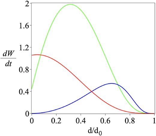
Rate of thermal energy release as a function of source separation d for the fin current sheet model, with |$C=\alpha /M_{\mathrm{ A}0}=0.1,$| 1 and 5 (red, green, and blue, respectively).
3 A FLOATING CURRENT SHEET
3.1 General treatment and numerical solution
The so-called ‘floating current sheet’ occurs when reconnection is initiated after a null point has formed in the corona, as studied previously by Priest et al. (2018) and Syntelis et al. (2019). However, they assumed that d is close to its initial value |$d_N$|, say, so that the magnetic field is close to potential and the current sheet is very short (|$L\ll d$|). In this section, we therefore improve and generalize their analysis to long current sheets and non-potential magnetic fields so as to be able to compare the results for a floating current sheet with those of a fin current sheet.
The improved technique employed here for calculating the three unknown variables, namely, the current sheet length (L) and the inflow speed (|$v_i$|) and field (|$B_i$|) to the current sheet, may be compared with the earlier technique for short current sheets adopted by Syntelis et al. (2019) and Priest et al. (2018). Here, we simply use the two flux conditions above and below the sheet for L and |$B_i$| and then deduce |$v_i$| from the reconnection rate [|$v_i=\alpha v_{\mathrm{ A}i}$|, see equation (9) above]. The earlier technique assumed as the first condition that |$B_i=\textstyle {\frac{1}{2}}k L$|, where k comes from the form of the potential field near the null, and this gives the same result as equation (26) below. The second condition was that the time rate of change of flux ejected below or above the sheet is equal to the flux (|$v_iB_i$|) into the current sheet, which relates L to |$v_i$|. The final condition was the same as here, namely, |$v_i=\alpha v_{\mathrm{ A}i}$|.
Suppose the magnetic field is in a potential state with no current sheet when the source separation is |$d_N$| (Fig. 4a), so that its magnetic field in complex form is
where |$z=x+iy$|. This has a null point at |$y=y_N$| on the y-axis, where
and the magnetic field on the y-axis is
so that the magnitude of the magnetic flux below the null point is
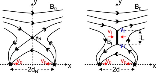
The nomenclature for a floating current sheet. (a) An initial potential state with a null point at height |$y_N\lt d_0$| due to two opposite-polarity sources a distance |$2d_N$| apart in a uniform horizontal field (|$B_0$|). (b) The field that is formed as the sources approach one another with speeds |$v_0$| to a separation distance of |$2d\lt 2d_N$|, giving rise to a current sheet of length L stretching from |$y_1$| to |$y_2$| on the y-axis, at which the inflow speed and magnetic field are |$v_i$| and |$B_i$|, respectively.
On the other hand, the total magnetic flux (|$\psi _\mathrm{ T}$|) across the y-axis is just
since a flux of amount F coming in from the left is diverted into the negative source. The magnetic flux above the null point is therefore
since an extra flux of magnitude |$\psi _N$| has been reconnected across the null point into the regions above and below it. Although this integral is infinite in view of the uniform field |$B_0$| extending to infinity, it is useful to recast it as
where |$F=\textstyle {\frac{1}{2}}\pi B_0 d_0$|.
Then suppose the sources approach one another at speeds |$v_0$|, so that their separation is |$2d$| and a current sheet of length L forms, stretching along the y-axis from |$y_1$| to |$y_2$| (Fig. 4b). Then the magnetic field may be represented by
so that along the y-axis
The current sheet endpoints (|$y_1$| and |$y_2$|) and therefore the length L of the current sheet are then given by the conservation of flux above and below the current sheet, namely,
where an argument similar to deriving equation (18) has been used. Here, |$B_x(0,y)$| is given by equations (19) and (21), |$\psi _N$| by equation (17), and the reconnected flux (|$F_\mathrm{ R}$|) by an equation similar to equation (10), namely,
with |$C=\alpha v_{A0}/v_0$|. In this expression for |$F_\mathrm{ R}$|, the function |$B_i(d)$|, namely, the field just outside the midpoint (|$y_N$|) of the current sheet, is given by the value of |$B_y$| from equation (20) evaluated at |$y_N=\textstyle {\frac{1}{2}}(y_1+y_2)$|, namely,
Thus, |$B_i$| and L are given by the coupled equations (22), (23), and (24). The resulting solutions can be obtained numerically as follows. When |$d=d_0$|, |$y_1=y_2=y_N$|, and |$F_\mathrm{ R}=0$|. Starting from these values, d is decreased by small increments from |$d=d_0$| to |$d=0$|. For each value of d the pair of equations in equation (22) is solved for |$y_1$| and |$y_2$| using the fsolve command in mapleTM.1 These values are then used to find |$B_i$| from (24) and then to update |$F_\mathrm{ R}$| from (23), following which d is decreased by a small increment and the process repeated. The numerical solutions are plotted in Fig. 5 for |$d_N=0.5 d_0$| and |$C=0$|, 0.1, 1, and 5. In the limit as the current sheet length becomes small compared with the flux interaction distance (|$L \ll d_0$|), we show in the following section that these reduce to
as in Syntelis et al. (2019), and
where
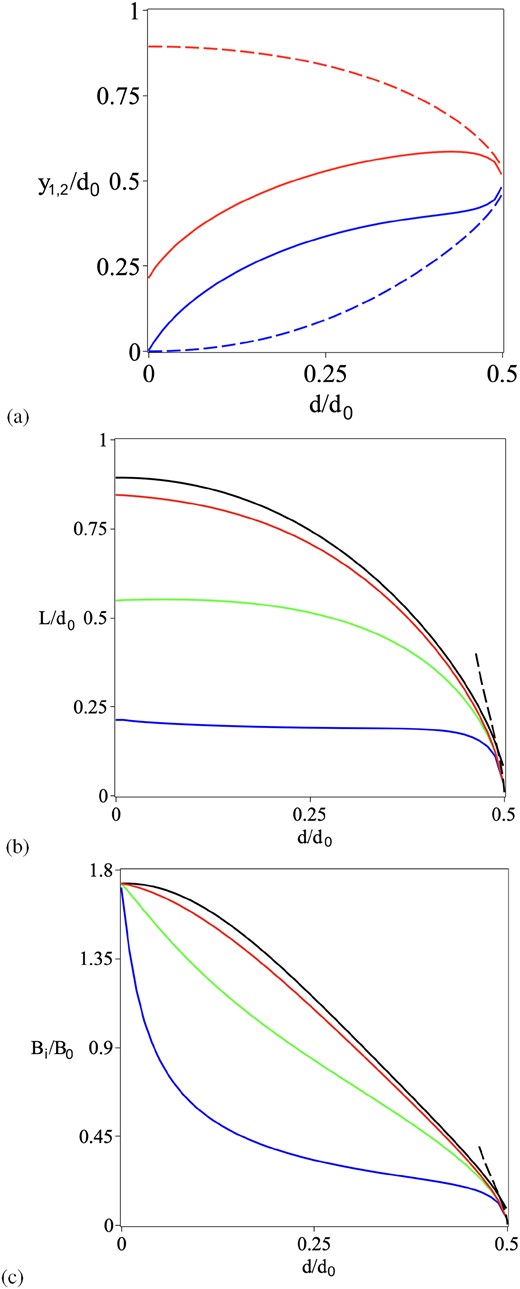
Parameters of the current sheet for the floating sheet model when the initial source separation (|$2d_N$|) equals |$d_0$| (so that |$d_N=\textstyle {\frac{1}{2}}d_0$|), where |$d_0$| is the flux interaction distance. (a) The endpoints |$y_1$| (blue) and |$y_2$| (red) of the current sheet in the absence of reconnection (|$C=0$|, dashed curves) and for |$C=5$| (solid curves). (b) The length (L) of the floating current sheet (|$L=y_2-y_1$|), as well as (c) the magnetic field (|$B_i$|) at the input to the current sheet, for |$C=0$| (black), |$C=0.1$| (red), |$C=1$| (green), and |$C=5$| (blue). The approximations when d is close to |$d_N$| (for |$C=0$|) are shown as dashed curves in parts (b) and (c).
The rate of energy release is given by the same expression as for the fin current sheet, namely, equation (15), but with |$B_i$| and L now given by equations (22)–(24). It is plotted in Fig. 6a for |$C=$|0.1, 1, and 5.
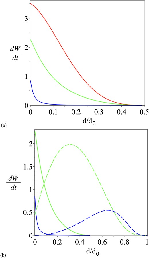
(a) The rate of energy release for a floating current sheet with |$d_N=\textstyle {\frac{1}{2}}d_0$| and |$C=0.1, 1, 5$|. (b) Comparison of the energy release rate for a fin current sheet (dashed) and floating current sheet (solid lines) for |$C=1$| (green) and |$C=5$| (blue).
3.2 The current sheet length and inflow magnetic field when the sheet is short
Consider the floating current sheet illustrated in Fig. 4. Initially, the source separation is |$2d_N$| and the magnetic field (16) is
which is potential and possesses a null point at height |$y_N$| given by
The magnetic flux (17) below the null point can be written
When the sources approach one another to a separation |$2d\lt 2d_N$|, a vertical current sheet forms stretching from |$z_1$| to |$z_2$| on the y-axis (Fig. 4b), and the magnetic field becomes
The resulting flux below the current sheet can then be written
where |$F_\mathrm{ R}$| is the reconnected flux.
The value of the current sheet length when d is close to |$d_N$|, so that the sheet length (L) is much smaller than |$d_N$|, is given by equating the two fluxes |$\psi _N$| and |$\psi _\mathrm{ S}$| and linearizing by writing |$y_1=y_N-Y_1$|, |$y_2=y_N+Y_2$|, and |$d=d_N-D$|, where |$Y_1\ll y_N$|, |$Y_2\ll y_N$|, and |$D\ll d_N$|. Then, equating |$\psi _\mathrm{ S}$| and |$\psi _N$| and omitting |$F_\mathrm{ R}$| since it is of higher order in the small quantities than those we shall ultimately keep,
After subtracting the integral of the initial flux up to |$y=y_1$| from both sides, this may be rewritten
where
which are evaluated in Appendix C, and
Each of these integrals is small, and, since |$I_B \sim L^2y_N\log _e L/(d_0d_N)$|, |$I_C \sim D$|, and |$I_A \sim L^2 y_N/(d_0d_N)$|, we shall to lowest order neglect |$I_A$| compared with the other two integrals. Thus, equating the expressions (C1) for |$I_B$| and (C2) for |$I_C$| in Appendix C, we obtain the result that
so that the current sheet length (L) in the combination |$L^2 \log _e L$| is proportional to the small displacement (D) of the sources from |$d_N$|, where |$f(d_N/d_0)$| is given by equation (C3). When |$d_N$| is close to |$d_0$|, this is well behaved, since the expression for L behaves like
which is plotted as the dashed curve in Fig. 5b.
Furthermore, equation (24) for the magnetic field at the inflow to the current sheet, namely,
may be approximated to lowest order for short current sheets when |$L \ll d_0$|, by putting |$y_2-y_1\approx L$|, |$y_2+3y_1 \approx 3y_2+y_1 \approx 4y_N$|, and |$y_1+y_2\approx 2y_N$|, so that
where |$y_N^2=d_0d_N-d_N^2$|, so that we recover the same expression as in Syntelis et al. (2019), namely,
which is plotted as the dashed curve in Fig. 5c.
4 CONCLUSION
Observations from the Sunrise balloon mission (Smitha et al. 2017; Solanki 2017) and more recently from the Solar Orbiter and Solar Probe missions have raised the possibility that magnetic reconnection driven by photospheric flux cancellation may be providing an important contribution to the heating of the Sun’s atmosphere and the acceleration of the solar wind, as suggested by Pontin et al. (2024) building on previous proposals (Peter et al. 2019; Chitta et al. 2020; Chen et al. 2021; Panesar et al. 2021; Tripathi, Nived & Solanki 2021; Raouafi et al. 2023).
The main implication of the present work is that, when oppositely directed fragments of photospheric magnetic flux approach one another, in the build-up to flux cancellation they may drive the formation of a current sheet between them, and so give rise to the heating and jets of plasma that could contribute to heating the chromosphere and corona and accelerating the solar wind. Previous analyses of energy release by such flux cancellation (Priest et al. 2018; Syntelis et al. 2019; Priest & Syntelis 2021; Syntelis & Priest 2021) have demonstrated that, based on newly observed flux cancellation rates, the process can provide a significant contribution to heating the chromosphere and corona. Here, we showed that cancellation at a fin current sheet – consistent with observations of energy release in the low atmosphere – is likely to be even more effective and produce much more heating. Furthermore, since the heating scales roughly as the square of the sheet length, dropping the assumption of a small current sheet also leads to much more heating in a floating current sheet than before. The net result of this theory is to put the suggestion of coronal heating by reconnection driven by flux cancellation on a much firmer foundation. In future, it will be interesting to compare with simulations designed to analyse the process in more detail.
The previous theory for reconnection by flux cancellation (Priest et al. 2018; Syntelis et al. 2019; Priest & Syntelis 2021; Syntelis & Priest 2021) made two assumptions that we improve upon here. The first was that the current sheet develops about a coronal null point, to give a so-called ‘floating current sheet’. However, whereas the flux from opposite-polarity flux fragments will not be connected when they are so far apart that their separation distance exceeds the flux interaction distance (|$d\gt d_0$|), as soon as it becomes equal (|$d=d_0$|) and decreases further (|$d\lt d_0$|) a null point (or separator) will form in the solar surface and a vertical current sheet will develop and grow. This type of current sheet we term a ‘fin sheet’ and analyse its growth for the first time here. If there is no reconnection, it will grow in length as the flux sources approach, up to a maximum length of |$L=d_0$| as their separation tends to zero. At the same time, the magnetic field at the sheet increases from zero up to a maximum value of |$\sqrt{3}B_0$|, where |$B_0$| is the overlying field strength.
When reconnection takes place, the sheet length and inflow magnetic field are smaller, as shown in Fig. 2, while the rate of energy release varies in a way shown in Fig. 3 and is usually larger than the rate from a floating current sheet. Examining Fig. 6(b) we see that for the chosen parameters the rate of energy release for the fin current sheet remains larger than the floating sheet until the flux patches are very close to one another (while |$d/d_0\gtrsim 0.1$|). Integrating the area under the curves in Fig. 6(b) (and dividing by |$v_0=\mathop {}\!\mathrm{d}d/\mathop {}\!\mathrm{d}t$|) allows the total energy released during the interaction to be quantified. For |$C=1$| the fin current sheet releases approximately a factor of 5 more energy (|$105.0/v_0$| compared with |$26.2/v_0$| in non-dimensional units), while for |$C=5$| the difference is nearly a factor of 10 (|$23.67/v_0$| compared with |$2.52/v_0$|).
The second assumption of previous theory that we focus on here is that a floating current sheet possesses a very small length (much smaller than its altitude). In Section 3, we dropped this assumption and allowed the sheet length to grow to a substantial fraction of the flux interaction distance (|$d_0$|), the actual value depending on the rate of reconnection, as shown in Fig. 5b. Meanwhile, the inflow field strength also varies and becomes of order the overlying field strength as the separation between the flux sources decreases (Fig. 5c). At the same time, the rate of energy release grows as the flux sources approach one another, reaching a maximum value at the moment of flux cancellation (Fig. 6a).
One argument for the existence of a floating current sheet is that the approach of nearby photospheric flux fragments of opposite polarity may be an intermittent process, so that the reconnection could start and stop, allowing the current sheet to dissipate completely before restarting as the null point (or separator) rises in the atmosphere. Another argument is that such sheets will naturally form when new motions of photospheric flux sources occur in fields that are already topologically complex with null points or separators present.
Here on grounds of simplicity, we have discussed current sheet formation in simple, idealized, two-dimensional magnetic fields affected by simple boundary flows, but the results are highly informative for the likely behaviour of topologically much more complex solar magnetic fields of a non-potential three-dimensional nature. First of all, current sheets may also form and be the location of magnetic reconnection and energy release in non-potential magnetic fields (e.g., Longcope 2005; Priest 2014; Pontin & Priest 2022). Furthermore, they may form around both null points and separators in three-dimensional magnetic fields of complex topology, as well as around quasi-nulls and quasi-separators in magnetic fields of simple topology (i.e., in the absence of nulls or separators) but complex geometry (e.g., Longcope 2005; Priest 2014; Pontin & Priest 2022). In addition, in a complex configuration with complex boundary flows, the resulting current sheets may have arbitrary inclination and be curved. Analysing such complex situations in future by both analytical and computational means will be a challenge but will hopefully be helped by the understanding developed here.
ACKNOWLEDGEMENTS
The authors thank the anonymous referee for constructive suggestions which have helped to improve the paper. DP gratefully acknowledges support through an Australian Research Council Discovery Project (DP210100709).
DATA AVAILABILITY
No new data were generated or analysed in support of this research.
Footnotes
Maple is a trademark of Waterloo Maple Inc.
REFERENCES
APPENDIX A: THE SOLUTION FOR |$L(d)$| FOR THE FIN CURRENT SHEET
Equation (6) is of the form
where,
and |$c=d^2/L^2$|. Changing the variable from u to U, where |$u^2=U^2+1$|, we find
or
or
Thus, equation (A1) becomes
or
namely, equation (7), as required.
APPENDIX B: EVALUATION OF FIN SHEET LENGTH (L) WHEN C SMALL OR LARGE
The fin sheet length (L) is given by equation (13). When |$C=\alpha /M_{A0}$| is so small that |$6C/\pi =\epsilon _1\ll 1$|, the solution for L is close to |$L_0=(d_0-d)^{1/2}$|, and so may be written |$L=L_0+\epsilon _1L_1$|, where
As d tends to zero, we see that |$L_1$| tends to |$-5(\pi /2 +1)/16$|.
On the other hand, when C is so large that |$\epsilon _2=\pi /(6C)\ll 1$|, there is a boundary layer near |$d=d_0$| of width |$\delta = (1/2) \epsilon _2^{1/2}d_0$|, such that |$L = \epsilon _2^{1/4} d$| when |$0\lt d \lt (1-\delta)d_0$| and |$L=(d_0^2-d_0d)^{1/2}$| when |$1-\delta \lt d/d_0 \lt 1$|. The result of numerically integrating equation (13) with this initial condition for different values of the constant C is shown in Fig. 2(a) with the corresponding values of the inflow field |$B_i$| to the current sheet (equation 12) in Fig. 2(b).
APPENDIX C: EVALUATION OF THE INTEGRALS |$I_B$| AND |$I_C$|
The integral |$I_B$| may be evaluated by assuming |$Y_2=Y_1$| and changing the variable from y to Y, where |$y_N-y=\textstyle {\frac{1}{2}}LY$|, so that it becomes
which is dominated by values near the upper limit (|$2y_N/L \gg 1$|), where |$(Y^2-1)^{1/2} \approx Y-1/(2Y)$| and the denominator approximates to |$4(y_N^2+d_N^2)/L^2=4d_0d_N/L^2$|. Thus the integral may be approximated by
or
where |$y_N/d_N=(d_0/d_N-1)^{1/2}$|, so that
Next, the integral |$I_C$| may be written
or
where
and
and so, after some manipulation, our integral becomes
where
