


ABSTRACT
The accreting millisecond X-ray pulsar IGR J17498−2921 went into X-ray outburst on 2023 April 13–15, for the first time since its discovery on 2011 August 11. Here, we report on the first follow-up NuSTAR observation of the source, performed on 2023 April 23, around 10 d after the peak of the outburst. The NuSTAR spectrum of the persistent emission (3–60 keV band) is well described by an absorbed blackbody with a temperature of |$kT_{\mathrm{ bb}}=1.61\pm 0.04$| keV, most likely arising from the NS surface and a Comptonization component with power-law index |$\Gamma =1.79\pm 0.02$|, arising from a hot corona at |$kT_{e}=16\pm 2$| keV. The X-ray spectrum of the source shows robust reflection features which have not been observed before. We use a couple of self-consistent reflection models, relxill and relxillCp , to fit the reflection features. We find an upper limit to the inner disc radius of |$6\: R_{\mathrm{ ISCO}}$| and |$9\: R_{\mathrm{ ISCO}}$| from relxill and relxillCp model, respectively. The inclination of the system is estimated to be |$\simeq 40^{\circ }$| from both reflection models. Assuming magnetic truncation of the accretion disc, the upper limit of magnetic field strength at the pole of the NS is found to be |$B\lesssim 1.8\times 10^{8}$| G. Furthermore, the NuSTAR observation revealed two type-I X-ray bursts and the burst spectroscopy confirms the thermonuclear nature of the burst. The blackbody temperature reaches nearly 2.2 keV at the peak of the burst.
1 INTRODUCTION
An accreting millisecond pulsar (AMSP) is a neutron star (NS) accreting mass from a low-mass (|$\lesssim1 \mathrm{ M}_{\odot }$|) donor/companion star and showing a coherent signal with a period of few ms (Campana & Di Salvo 2018; Di Salvo & Sanna 2022). They are a high observational priority due to their rarity. To date, only 27 AMSPs have been discovered since 1998. SAX J1808.4−3658 is the first discovered AMSP (Wijnands & van der Klis 1998), the recent ones being MAXI J1816−195 (Bult et al. 2022b) and MAXI J1957+032 (Ng et al. 2022). Very recently Mereminskiy et al. (2024) reported the discovery of an AMSP SRGA J144459.2−604207 on 2024 February 21, by the ART-XC telescope. NS low-mass X-ray binaries (LMXBs) emit X-rays due to the accretion of matter from the companion star on to the NS through Roche lobe overflow. The pulsation is caused by the NS magnetic field, which is strong enough to funnel the accreting matter to the magnetic poles effectively. NS LMXBs are classified into persistent and transient sources based on long-term X-ray variabilities. Persistent NS LMXBs accrete matter continuously and may have an X-ray luminosity of |$L_{X}\gtrsim 10^{36} {\rm ~erg\ s}^{-1} {}$| (Ludlam et al. 2017, 2019 ). On the contrary, transient LMXBs do not accrete matter continuously and undergo recurrent bright (|$L_{X}\gtrsim 10^{36} {\rm ~erg\ s}^{-1} {}$|) outbursts lasting from days to weeks and then return to prolonged intervals of X-ray quiescence (|$L_{X}\lesssim 10^{34} {\rm ~erg\ s}^{-1} {}$|) lasting from months to years (Degenaar & Wijnands 2010; Di Salvo & Sanna 2020). Most of the AMSPs are transient X-ray sources with recurrence times between 2 and more than 10 yr, and their outbursts usually last from a week to a few months (Patruno & Watts 2020). Almost all AMSPs have short, i.e. |$\sim$|hours or minutes, orbital periods and are therefore characterized by compact orbits. Most of these systems are bursters, as they have displayed a type-I thermonuclear X-ray burst at least once (Papitto et al. 2010; Di Salvo et al. 2019; Galloway & Keek 2021; Bult et al. 2022a; Ng et al. 2024). The bursts from AMSPs exhibit burst oscillations at the typical spin frequency (Patruno & Watts 2020).
From a spectral point of view, the emission from these systems in outburst is usually dominated by the Comptonization spectrum from a hot corona with electron temperatures usually of tens of keV (Di Salvo & Sanna 2022). AMSPs in outburst are, therefore, (almost) always in a hard spectral state. The accretion flow is expected to stop far from the NS surface in this state. However, two AMSPs, SAX J1748.9−2021 and SAX J1808.4−3658, have been observed to transition into the soft states (Pintore et al. 2016; Di Salvo et al. 2019). Besides an energetically dominating Comptonized component, one or two soft components with relatively low temperatures are often detected depending on the statistics and spectral resolution of the detectors. These soft components are interpreted as the emission arising from the accretion disc and the NS surface/boundary layer. An additional spectral component arises when the Comptonization spectrum emitted by the corona illuminates the disc and is reprocessed by it. This component is known as the reflection spectrum, a prevalent ingredient in spectra of X-ray binaries (Fabian et al. 1989). Disc reflection components are mainly characterized by a Fe–K emission line at |$\simeq 6.4-6.97$| keV and a Compton hump at |$\simeq 20-40$| keV (Fabian et al. 1989). X-ray reflection spectroscopy provides a powerful diagnostic tool for investigating the dynamics and geometry of the accretion disc. Detecting and modelling disc reflection features allow for a measure of the inner radial extent of the accretion disc, the ionization of the plasma in the disc, and the inclination of the system. Reflection features have been observed in some AMSPs for which data with high-to-moderate energy resolution were available (Papitto et al. 2013; Sanna et al. 2017; Di Salvo et al. 2019; Marino et al. 2022) but not all (Falanga et al. 2005; Sanna et al. 2018a, b).
IGR J17498−2921 is known as an AMSP, discovered with INTEGRAL on 2011 August 11, (Gibaud et al. 2011). The source position was determined by follow-up Swift (Bozzo et al. 2011) and Chandra (Chakrabarty et al. 2011) observations. The source is located at α = 17h49m55|${_{.}^{\rm s}}$|35, |$\delta =-29^{^{\circ }}19^{^{\prime }}19{_{.}^{\prime\prime}}6^{^{ }}$|, with an associated uncertainty of 0.6 arcsec at the |$90{{\ \rm per\ cent}}$| confidence level. Pulsation at a frequency of |$\sim 401$| Hz was observed from this source (Papitto et al. 2011b). The source resides in a 3.8 hr binary (Markwardt, Strohmayer & Smith 2011), orbiting a low-mass companion donor with mass |$\sim 0.2 \mathrm{ M}_{\odot }$| (Galloway et al. 2024). Thermonuclear X-ray bursts were detected by Ferrigno, Bozzo & Belloni (2011) during INTEGRAL observations of this source. Linares et al. (2011a) reported burst oscillations from this source at a frequency consistent with the spin frequency. Burst oscillation from this source was further confirmed by Chakraborty & Bhattacharyya (2011) using RXTE/PCA data with a much higher significance. Bursts from this source also show the characteristics of the photospheric radius expansion episode, which gives a distance estimate of |$\sim 7.6$| kpc (Linares et al. 2011a). After a 37-d-long outburst, the source returned to quiescence on 2011 September 19, (Linares et al. 2011b). The source was observed at a luminosity of |$\sim 2\times 10 ^{32}$| erg s|$^{-1}$| during quiescence (Jonker et al. 2011). From the current INTEGRAL observation performed on 2023 April 13–15, the source was again found in a bright X-ray state for the first time since its discovery in 2011 (Grebenev, Bryksin & Sunyaev 2023). NICER observation also confirms the new outburst from this source (Sanna et al. 2023).NICER follow-up observations starting on 2023 April 19, detected the source at a constant count rate of |$\sim 80$| ct s−1 in the |$0.5-10$| keV band (Sanna et al. 2023). Later, Nuclear Spectroscopic Telescope ARray (NuSTAR) observed the source on 2023 April 23, around 10 d after the peak of the outburst. We used the NuSTAR observation for our analysis.
Papitto et al. (2011a) analysed the spectral properties of IGR J17498−2921 based on the observations performed by the SWIFT and the RXTE/PCA between 2011 August 12 and September 22. During most of the outburst, the spectra are modelled by a power-law with an index |$\Gamma \approx 1.7-2$|, while values of |$\approx 3$| are observed as the source fades into quiescence. Later, Falanga et al. (2012) studied the broad-band spectrum of the persistent emission in the |$0.6 - 300$| keV energy band using simultaneous INTEGRAL, RXTE, and SWIFT data obtained in 2011 August–September. They also discussed the properties of the largest set of X-ray bursts from this source discovered by these satellites. They found that the broad-band average spectrum is well-described by thermal Comptonization with an electron temperature of |$kT_{e}\sim 50$| keV, soft seed photons of |$kT_{\mathrm{ bb}} \sim 1$| keV, and Thomson optical depth |$\tau _{T} \sim 1$| in slab geometry. The INTEGRAL, RXTE, and SWIFT data also reveal the X-ray pulsation at a period of 2.5 ms up to |$\sim 65$| keV (Papitto et al. 2011a). Sanna et al. (2023) reported on the recent NICER observation of this source performed on 2023 April 19, and they found that the |$1-10$| keV energy spectrum is well described using an absorbed blackbody and a Comptonization continuum (nthcomp). They also found a blackbody temperature of |$\sim 0.30$| keV, and a Comptonization power-law index of |$\sim 1.76$|. They estimated the |$0.5-10$| keV unabsorbed flux at |$\sim 1\times 10^{-9}$| erg s|$^{-1}$| cm|$^{-2}$|, which matches the 2011 peak flux.
In this work, we represent the spectral analysis of the persistent emission of this source using the available NuSTAR observation performed on 2023 April 23. We also investigate the properties of the type-I X-ray bursts from this source. Due to unprecedented sensitivity above 10 keV, it is possible to constrain the accretion geometry of the system by modelling the reflection spectrum (Fabian et al. 1989) using NuSTAR. Moreover, fitting with self-consistent reflection models will give important information on the position of the magnetospheric radius and the NS magnetic field. We have organized the paper as follows: we provide an overview of the observation and data reduction in Section 2. We present the source light curves in Section 3. We provide the details of the spectral analysis, both persistent and burst emission, in Section 4. Finally, we discuss the results obtained from the analysis in Section 5.
2 OBSERVATION AND DATA REDUCTION
NuSTAR (Harrison et al. 2013) observed the source IGR J17498−2921 only once on 2023 April 23, for a total exposure of |$\sim 45$| ks. We have used this observation (obsID: 90901317002) for our analysis.
The NuSTAR data were collected in the |$3-79$| keV energy band using two identical co-aligned telescopes equipped with the focal plane modules FPMA and FPMB.We reduced the data using the standard data analysis software nustardas v2.1.2 task included in heasoft v6.33.2. We used the latest NuSTARcaldb version available (|$v20240206$|) at the time of the analysis. We used the task nupipeline v0.4.9 to generate the calibrated and screened event files. The source events have been extracted from a circular region centred on the source position, with a radius of 120 arcsec for both detectors FPMA and FPMB. The background events also have been extracted from a circle of the same radius from the area of the same chip but in a position far from the source for both instruments. The filtered event files, the background-subtracted light curves, and the spectra for both detectors are extracted using the tool nuproducts. Corresponding response files are also created as output of nuproducts, which ensures that all the instrumental effects, including loss of exposure due to dead-time, are correctly accounted for. We grouped the FPMA and FPMB spectral data with a minimum of 100 counts per bin which allows the use of |$\chi ^{2}$| statistics. Finally, we fitted spectra from detectors FPMA and FPMB simultaneously, leaving a floating cross-normalization constant.
3 LIGHT CURVE
In the left panel of Fig. 1, we show the NuSTAR/FPMA light curve of the source in the |$3-79$| keV energy band during the decay of the 2023 outburst. The average count rate during the NuSTAR observation was |$\sim 20-24$| counts s|$^{-1}$| (see right panel of Fig. 1). Two type-I thermonuclear X-ray bursts were present at about |$\sim 31$|st and |$\sim 64$|th ks during the NuSTAR observation. Those are marked with the green vertical boxes. This is the first detection of X-ray bursts in the 2023 outburst cycle as no bursts have been reported by the previous INTEGRAL and NICER observations. The peak of the burst seems to reach approximately |$\sim 680$| counts s|$^{-1}$|, about a factor of |$\sim 28$|, the level of the persistent emission. Both type-I bursts lasted about |$\sim 20$| s. We have extracted the light curve and spectrum of the bursts and investigated the properties in details. For the persistent emission spectrum, we eliminated a time interval of around 1000 s surrounding the burst, starting from 250 s before the rise of the burst.
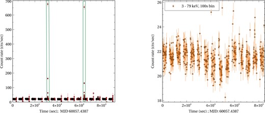
Left panel: |$3-79{\rm ~keV}{}$|NuSTAR/FPMA light curve of the source with a binning of 10 s. The source shows the presence of two thermonuclear X-ray burst. Right panel: same light curve with a binning of 100 s after removing burst intervals.
4 SPECTRAL ANALYSIS
We used the X-ray spectral package xspec v12.14.0h (Arnaud 1996) to model the NuSTAR FPMA and FPMB spectra simultaneously between 3 to 60 keV energy band, while above 60 keV spectrum is dominated by the background. A constant multiplication factor constant was included in the modelling to account for cross-calibration of the two instruments, FPMA and FPMB. The value of constant for FPMA was fixed to 1, allowing it to vary for the FPMB. We used the TBabs model to account for interstellar absorption along the line of sight with the wilm abundances (Wilms, Allen & McCray 2000) and the vern (Verner et al. 1996) photoelectric cross-section. Unless otherwise stated, spectral uncertainties are quoted at the |$1 \sigma$| confidence level.
4.1 Continuum modelling
Different combinations of model components and spectral parameters are required to describe the continuum emission from different spectral states from the NS LMXBs. To probe the spectral shape of this source correctly, we first tried to fit the continuum emission (NuSTAR spectrum |$3-60$| keV) with a model consisting of an absorbed cut-off power-law ( cutoffpl) and a single-temperature blackbody component (bbody). These models describe the emission from the presence of the corona and surface of the NS and/or boundary layer region, respectively. This standard model combination has previously been used to fit the broad-band continuum emission in AMSPs (Di Salvo & Sanna 2022). This two-component model describes the continuum emission reasonably well. The poor quality of the fit (|$\chi ^2/dof=1561/1273$|) is mainly due to the presence of strong reflection features in the |$5-9$| keV and |$12-30$| keV energy range. Because of the lack of sensitivity of NuSTAR at low energies, we had to fix the photoelectric equivalent hydrogen column density at |$0.81 \times 10^{22}$| cm|$^{-2}$|, following Dickey & Lockman (1990). We found that the spectrum is dominated by a hard Comptonization component from the corona with a photon index of |$\Gamma =1.70\pm 0.02$| and the cut-off energy |$E_{\mathrm{ cut}}= 55\pm 4$| keV. The cut-off power-law component accounts for |$\simeq 88{{\ \rm per\ cent}}$| of the total |$3 - 79$| keV unabsorbed flux. The inferred blackbody temperature |$kT_{\mathrm{ bb}}= 1.55\pm 0.03{\rm ~keV}{}$| suggests that this continuum may originate from the NS surface and/or boundary layer region.
A much better description of continuum emission due to thermal Comptonization is given by the model nthcomp (Zdziarski, Johnson & Magdziarz 1996). It attempts to simulate the upscattering of photons through the corona from a seed spectrum parametrized either by the inner temperature of the accretion disc or the NS surface/boundary layer. Both shapes can be selected via the input type, parametrized by a seed photon temperature. The high energy cut-off is parametrized by the electron temperature of the medium. We then replaced the cut-off power-law model with the physically motivated Comptonization model nthcomp, setting the photon seed input to a disc blackbody. This model also describes the continuum emission very well with |$\chi ^2/dof=1495/1272$|. We estimated the electron temperature at |$kT_{e}= 16\pm 2{\rm ~keV}{}$| with photon index |$\Gamma = 1.79\pm 0.02$|. The seed photon temperature is found to be low |$kT_{\mathrm{ seed}}\lesssim 0.31{\rm ~keV}{}$|, indicating the difficulties in detecting the additional soft disc blackbody component separately arising from the accretion disc. The electron temperature of the corona, |$kT_{e}$|, is roughly comparable to the observed cut-off energy (|$\sim 55$| keV) of the spectrum. The optical depth of the corona is found to be |$\tau = 4.0\pm 0.2$| for the nthcomp model, suggesting an optically thin corona. Therefore, seed photons of temperature lower than |$\approx 0.31$| keV are Comptonized in a corona with an electron temperature of |$\sim 16$| keV and an optical depth of |$\sim 4.0$|, corresponding to a photon index of the Comptonized spectrum of |$\Gamma \sim 1.8$|.
Our continuum description with different combinations of the model leaves large positive residuals around |$5-9$| and |$12-30$| keV, as shown in Fig. 2. It indicates the presence of a broad iron emission feature and Compton reflection hump, respectively. These features are typically attributed to disc reflection. This motivates the inclusion of a relativistic reflection model in our spectral fits.
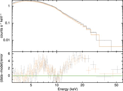
The source spectrum in the energy band |$3-60{\rm ~keV}{}$| obtained from the NuSTAR FPMA and FPMB is presented here. The continuum emission is fitted with the absorbed bbody and the nthcomp model. Fit ratio associated with this continuum model is shown in the bottom panel of this plot. The presence of disc reflection is evident in the spectrum.
4.2 Self-consistent reflection fitting
4.2.1 Reflection fits with relxill
When hard X-rays irradiate the accretion disc, they produce a reflection spectrum that includes fluorescence lines, recombination, and other emission (Fabian et al. 1989). The shape of the reflection spectrum depends on the properties of the flux incident on the accretion disc. In most X-ray sources, the illuminating continuum input is generally a hard power-law spectrum. However, in NS systems, the emission from the NS surface/boundary layer may be significant and contribute to the reflection (Cackett et al. 2008; Ludlam et al. 2019, 2017). In the case of IGR J17498−2921, the X-ray spectrum is dominated by a power-law component. We choose the reflection model relxill to reproduce both Comptonization and reflection emission correctly. It has a cut-off power-law with photon index |$\Gamma$| and cut-off energy |$E_{\mathrm{ cut}}$| as the illuminating photon distribution. The model combines the reflection grid xillver (García et al. 2013) with the convolution kernel relconv to include relativistic effects on the shape of the reflection spectrum (Dauser et al. 2010).
The model parameters of relxill are as follows: the inner and outer disc emissivity indices |$q_{1}$| and |$q_{2}$|, respectively, the break radius |$R_{\mathrm{ break}}$| which sets the location in the disc where the emissivity index changes from |$q_{1}$| to |$q_{2}$|, the inner and outer radii of the disc |$R_{\mathrm{ in}}$| and |$R_{\mathrm{ out}}$| in units of the ISCO (|$R_{\mathrm{ ISCO}}$|), respectively, the inclination angle i of the system wrt our line of sight, the dimensionless spin parameter a, the photon index of the input cut-off power-law |$\Gamma$|, the ionization parameter log|$\xi$|, the iron abundance of the system |$A_{Fe}$|, the cut-off energy |$E_{\mathrm{ cut}}$|, the reflection fraction |$r_{\mathrm{ refl}}$|, and the normalization of the model. During our fitting, we used a single emissivity profile (hence |$R_{\mathrm{ break}}$| is obsolete). We fixed the emissivity index at |$q_{1}=q_{2}=3$| (a value commonly found in X-ray binaries). The redshift of the source (z) is fixed at 0 as the source is Galactic one. We fixed |$a=0.19$| as the source has a spin frequency of 401 Hz (considering |$a\simeq 0.47/P_{\mathrm{ ms}}$| (Braje, Romani & Rauch 2000) where |$P_{\mathrm{ ms}}$| is the spin period in ms). The outer disc radius is fixed at |$R_{\mathrm{ out}}=1000\,\,R_{g}$| (where |$R_{g}=GM/c^2)$|. The parameters |$R_{in}$|, i, |$A_{Fe}$|, log|$\xi$|, |$\Gamma$|, |$E_{\mathrm{ cut}}$|, |$r_{\mathrm{ refl}}$| were left free to vary. The addition of the model relxill improved the fit significantly to |$\chi ^2/dof=1244/1268$| (|$\Delta \chi ^2=-317$| for the five additional parameters). The corresponding spectrum for the model constant*TBabs*(bbody+relxill) and the residuals are shown in the left panel of Fig. 3. The best-fitting parameters are reported in Table 1.
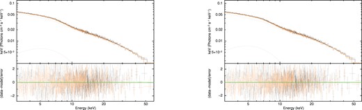
Left panel: the unfolded spectral data, the best-fitting model const*TBabs*(bbody+RELXILL). The lower panel of this plot shows the ratio of the data to the model in units of |$\sigma$|. Right panel: the unfolded spectral data, the best-fitting model const*TBabs*(bbody+RELXILLCP).
Fit results: best-fitting spectral parameters of the NuSTAR observation of the source IGR J17498−2921. Model 1: const*TBabs*(bbody+relxill) and Model 2: const*TBabs*(bbody+relxillCp).
| Component | Parameter (unit) | Model 1 | Model 2 |
|---|---|---|---|
| Constant | FPMB (wrt FPMA) | |$0.98\pm 0.003$| | |$0.98\pm 0.002$| |
| tbabs | |$N_{H}\, (\times 10^{22}\,\,\text{cm}^{-2}$|) | |$0.81$|(f) | |$0.81$|(f) |
| bbody | |$kT_{\mathrm{ bb}} \, ({\rm keV})$| | |$1.61_{-0.10}^{+0.21}$| | |$1.66_{-0.08}^{+0.13}$| |
| Norm (|$\times 10^{-3}$|) | |$1.01_{-0.12}^{+0.20}$| | |$1.11_{-0.12}^{+0.10}$| | |
| relxill/relxillCp | i (degrees) | |$37_{-7}^{+8}$| | |$40_{-8}^{+12}$| |
| |$R_{\mathrm{ in}}$| (|$\times R_{\mathrm{ ISCO}}$|) | |$\lesssim 6$| | |$\lesssim 9$| | |
| |$\rm {log}\:\xi$| (erg cm s|$^{-1}$|) | |$4.12_{-0.15}^{+0.10}$| | |$4.28_{-0.48}^{+0.07}$| | |
| |$\Gamma$| | |$1.68\pm 0.02$| | |$1.76\pm 0.03$| | |
| |$A_{Fe}$| (|$\times \,\,\text{solar})$| | |$\gtrsim 1.58$| | |$\gtrsim 2.14$| | |
| |$E_{\mathrm{ cut}}\, ({\rm keV})$| | |$105_{-20}^{+12}$| | – | |
| logN (cm|$^{-3}$|) | – | |$\lesssim 18$| | |
| |$kT_{e} \, ({\rm keV})$| | – | |$19_{-1}^{+2}$| | |
| |$f_{\mathrm{ refl}}$| | |$4.21_{-3.06}$|a | |$1.13_{-0.40}^{+1.32}$| | |
| norm (|$\times 10^{-4}$|) | |$3.80_{-1.21}^{+1.98}$| | |$9.29_{-2.3}^{+1.9}$| | |
| cflux | |$F_{\mathrm{ bbody}}$|b (|$\times 10^{-9}$| erg s−1 cm−2) | |$0.08\pm 0.02$| | |$0.09\pm 0.02$| |
| |$F_{\mathrm{ relxill}/\mathrm{ relxillCp}}$|b (|$\times 10^{-9}$| erg s−1 cm−2) | |$1.04\pm 0.01$| | |$1.03\pm 0.01$| | |
| |$F_{\mathrm{ total}}$|b (|$\times 10^{-9}$| erg s−1 cm−2) | |$1.12\pm 0.01$| | |$1.12\pm 0.01$| | |
| |$\chi ^{2}/dof$| | |$1244/1268$| | |$1242/1267$| |
Notes. The outer radius of the relxill/relxillC p spectral component was fixed to |$1000\,\,R_{g}$|. We fixed emissivity index |$q1=q2=3$|. The spin parameter (a) was fixed to 0.19 as the spin frequency of the NS is 401 Hz.
Upper bound error calculation is not well constrained.
All the unabsorbed fluxes are calculated in the energy band 3–79 keV using the cflux model component in xspec.
4.2.2 Reflection fits with relxillCp
There is a flavour of relxill with a Comptonization illuminating continuum known as relxillCp. The primary emission for this model is given by the Comptonized model nthcomp. However, model relxillCp assumes the seed photons arise from the accretion disk with a fixed temperature of 0.05 keV (Dauser et al. 2014). Since we find a low seed photon temperature lower than |$\sim 0.3$| keV in our continuum fit with nthcomp, we attempt to use relxillCp in our spectral fit. The model relxillCp has similar parameters as that of relxill with the addition of logN (cm|$^{-3}$|) to vary the density of the accretion disc with an upper limit of 20 and electron temperature (|$kT_{e}$|) of the Comptonizing plasma instead of |$E_{\mathrm{ cut}}$|. We kept some of the model parameters fixed during the fit as mentioned for the relxill model. This reflection model also improved the fit significantly to |$\chi ^2/dof=1242/1267$| (|$\Delta \chi ^2=-253$| for the five additional parameters). The corresponding spectrum for the model constant*TBabs*(bbody+relxillCp) and the residuals are shown in the right panel of Fig. 3. The best-fitting parameter values using both reflection models are consistent and fully compatible with each other. All the best-fitting parameter values are listed in Table 1. Previously, Di Salvo et al. (2019) employed this model successfully to describe the spectral properties of the known AMSP SAX J1808.4−3658.
Most interestingly, the reflection component implies a large disc truncation in both models: the |$1\:\sigma$| upper limit on |$R_{\mathrm{ in}}\simeq 6\:R_{\mathrm{ ISCO}}$| for the relxill model and |$R_{\mathrm{ in}}\simeq 9\:R_{\mathrm{ ISCO}}$| for the relxillCp model. Both models also yield a consistent, moderate inclination estimate of |$37^{\circ+8}_{-7}$| for the relxill model and |$40^{\circ +12}_{-8}$| for the relxillCp model. We estimated a high disc ionization of log|$\xi =4.12_{-0.15}^{+0.10}$|. The value is consistent with the typical range observed in NS LMXBs (log |$\xi \sim 3-4$|). Both reflection fits appear to favour a high Fe abundance. The |$1\:\sigma$| lower limit on Fe abundance lies |$\simeq 1.58$|. This could be indicative of a high density of the accretion disc. The relxillCp model predicted an upper limit of the disc density parameter of |$10^{18}$| cm|$^{-3}$|. The reflection fraction |$f_{\mathrm{ refl}}$| parameter represents the ratio of illuminating flux to that which is reflected for relxill and relxillCp. The value of reflection fraction |$f_{\mathrm{ refl}}$| is close to unity, as expected, since the majority of emitted photons would interact with the disc with relatively fewer emitted towards infinity.
Further, we have tested the goodness of the fit for the inner disc radius, |$R_{\mathrm{ in}}$|, and disc inclination angle, i. We used the command steppar in xspec to search the best-fitting for |$R_{in}$| and i for both best-fitting models const*TBabs*(bbody+relxill) and const*TBabs*(bbody+relxillCp). Left panel of Fig. 4 shows the variation of |$\Delta \chi ^{2}(=\chi ^{2}-\chi _{\mathrm{ min}}^{2})$| as a function of |$R_{\mathrm{ in}}$| for both models and right panel of Fig. 4 shows the variation of |$\Delta \chi ^{2}$| with i for both models.
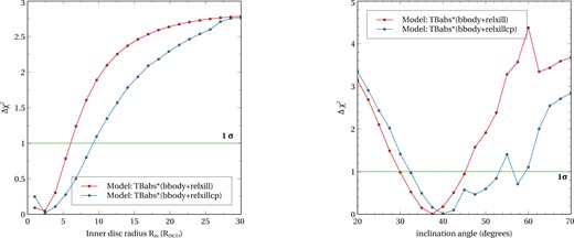
The plots show the change in the goodness of fit for the inner disc radius (|$R_{\mathrm{ in}}$|) and disc inclination angle (i). The left panel shows the variation of |$\Delta \chi ^{2}(=\chi ^{2}-\chi _{\mathrm{ min}}^{2})$| as a function of |$R_{\mathrm{ in}}$| (varied between 1 and |$30\:R_{\mathrm{ ISCO}}$|) obtained from two different model combination. The right panel shows the variation of |$\Delta \chi ^{2}(=\chi ^{2}-\chi _{\mathrm{ min}}^{2})$| as a function of i obtained from different models. We varied the disc inclination angle between 20° and 70°.
4.3 Type-I X-ray burst
During NuSTAR observation of IGR J17498−2921, two type-I thermonuclear bursts have been observed in the |$3-79$| keV light curve. We have performed an analysis of individual bursts and showed them in Figs 5 and 6. Both bursts have sharp rises and exponential falls and typically last 20 s. The rising part has hardly been detected because of its rapidness (|$\lt $|1 s). Therefore, we divided the burst into three segments: the peak of the burst (part-1; 5 s around the peak flux), the exponential fall (part-2; next 5 s after the peak), and the tail of the burst (part-3; last 10 s of the burst as it gradually flattens). Three segments of the bursts are shown by stars, circles, and triangles in the top left panel of Figs 5 and 6, respectively. We have created GTI files, extracted spectra, and performed analyses for three segments separately.
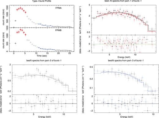
Top left: light curve profile of the first type-I burst is shown in 3–20 keV as observed by NuSTAR/FPMA (top) and NuSTAR/FPMB (bottom). The peak of the profile, the falling part, and the tail are shown in stars, circles, and triangles. FPMA and FPMB joint best-fitting spectra analysed during the peak profile, falling part, and the tail of burst-1 are shown in the top right, bottom left, and bottom right panels, respectively, along with the residuals.
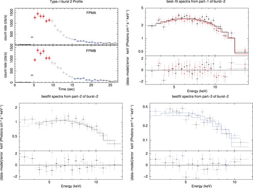
Top left: light curve profile of the second type-I burst is shown in 3–20 keV as observed by NuSTAR/FPMA (top) and NuSTAR/FPMB (bottom). The peak of the profile, the falling part, and the tail are shown in stars, circles, and triangles. FPMA and FPMB joint best-fitting spectra were analysed during the peak profile, the falling part and the tail of burst-2 are shown in the top right, bottom left, and bottom right panels, respectively, along with the residuals.
We found that burst spectra extracted from FPMA and FPMB during three segments can jointly be fitted by a single blackbody radiation (bbodyrad in xspec) in the presence of neutral absorption (TBabs in xspec). The blackbody nature of the burst has also been observed in several past studies. A constant is used to normalize the response between FPMA and FPMB. The absorption column density is kept fixed at |$0.81 \times$| 10|$^{22}$| cm|$^{-2}$|, which is the line-of-sight column density. Best-fitting spectral parameters for individual segments are provided in Table 2 for both bursts. The top right, bottom left, and bottom right panels of Figs 5 and 6 show best-fitting unfolded spectra along with residual during peak flux, exponential fall, and tail of both bursts, respectively.
Burst spectral analysis: best-fitting spectral parameters during three segments (Parts 1–3) of both bursts are provided. kT|$_{\mathrm{ bbody}}$| is the blackbody model temperature in keV, and BBodyNorm is the blackbody normalization.
| Burst | Part | kT|$_{\mathrm{ bbody}}$| | BBody | |$\chi ^2/dof$| |
|---|---|---|---|---|
| number | number | (keV) | Norm | |
| Part-1 | 2.19|$^{+0.05}_{-0.04}$| | 177|$^{+14}_{-13}$| | 62/63 | |
| BURST-1 | Part-2 | 1.78|$^{+0.05}_{-0.05}$| | 106|$^{+12}_{-11}$| | 36/34 |
| Part-3 | 1.38|$^{+0.04}_{-0.04}$| | 94|$^{+13}_{-11}$| | 23/27 | |
| Part-1 | 2.14|$^{+0.06}_{-0.05}$| | 204|$^{+17}_{-18}$| | 41/46 | |
| BURST-2 | Part-2 | 2.03|$^{+0.05}_{-0.05}$| | 93|$^{+13}_{-11}$| | 23/30 |
| Part-3 | 1.52|$^{+0.06}_{-0.06}$| | 76|$^{+12}_{-11}$| | 22/20 |
From Table 2, we may note that the blackbody temperature is highest during the peak of the burst and falls off significantly as the burst count falls towards the tail. Similarly, the blackbody emitting radius (a proxy for the blackbody normalization) is highest at the peak and becomes smaller as the flux decreases. A similar trend in temperature and radius has also been observed in other type-I X-ray bursts (Galloway et al. 2008; Galloway & Keek 2021; Bult et al. 2022a; Ng et al. 2024).
5 DISCUSSION
We present the results of the spectral analysis of the AMSP IGR J17498−2921 using the NuSTAR observation during its decaying phase of 2023 outbursts. During this observation, the source is detected with an average count rate of |$\sim 22{\rm ~count\ s}^{-1}$|. The unabsorbed |$3-79{\rm ~keV}{}$| flux is estimated at |$1.1\times 10^{-9}$| erg s|$^{-1}$| cm|$^{-2}$|, consistent to that of NICER flux in the |$0.5-10$| keV energy band observed on 2023 April 19 (Sanna et al. 2023). However, the unabsorbed bolometric X-ray flux during this observation in the energy band |$0.1-100{\rm ~keV}{}$| is |$1.32\times 10^{-9}$| erg s|$^{-1}$| cm|$^{-2}$|. This implies an unabsorbed bolometric luminosity of |$7.8\times 10^{36}$| erg s|$^{-1}$|, assuming a distance of 7.6 kpc. This value corresponds to |$\sim 2{{\ \rm per\ cent}}$| of the Eddington luminosity (|$L_{\mathrm{ Edd}}$|) which is |$\sim 3.8\times 10^{38}$| erg s|$^{-1}$| for a canonical |$1.4\:\mathrm{ M}_{\odot }$| NS (Kuulkers et al. 2003). The X-ray luminosity during outburst remains below |$10{{\ \rm per\ cent}}$| the |$L_{\mathrm{ Edd}}$| in the vast majority of the AMSPs. From the INTEGRAL data, maximum flux observed during the 2023 outburst was around |$4.7\times 10^{-9}$| erg s|$^{-1}$| cm|$^{-2}$| in the energy band |$28-84{\rm ~keV}{}$| (Grebenev et al. 2023). So, the unabsorbed source flux decays roughly four times within a short time-scales (a span of around 10 d). The peak flux observed during the 2011 outburst in the 2–30 keV energy band was |$\sim 1.1\times 10^{-9}$| erg s|$^{-1}$| cm|$^{-2}$|, smaller than the 2023 peak outburst flux.
We found that the continuum X-ray emission is well described using an absorbed blackbody (|$kT_{\mathrm{ bb}}=1.55 \pm 0.03{\rm ~keV}{}$|) and a power-law (|$\Gamma = 1.70\pm 0.02$|) with a cut-off energy at |$55\pm 4 {\rm ~keV}{}$|. The combination of absorbed blackbody and a physically motivated Comptonization model nthcomp also described the continuum fairly well with electron temperature |$kT_{e}=16\pm 2{\rm ~keV}{}$|, photon index |$\Gamma = 1.79\pm 0.02$|, and the seed photon temperature |$kT_{\mathrm{ seed}}\lesssim 0.31{\rm ~keV}{}$| likely originating from the disc. Thus, to describe the continuum emission of IGR J17498−2921, we need a single blackbody component of temperature |$kT_{\mathrm{ bb}}\simeq 1.6{\rm ~keV}{}$|, likely arising from the NS surface and a Comptonization spectrum which can be associated with a hot corona scattering of photons from a cold disc of temperature |$kT_{\mathrm{ seed}}\lesssim 0.31{\rm ~keV}{}$|, whose direct emission is likely too faint for detection. The blackbody parameters (|$kT_{\mathrm{ bb}}\sim 1.6$| keV, |$R_{\mathrm{ bb}}\sim 1.1-1.2$| km) suggest that this continuum might originate from a small part of the NS surface. From continuum mode-lling, we found that the spectrum is dominated by a hard Comptonization component, comprising of |$\simeq 88{{\ \rm per\ cent}}$| of the total |$3 - 79$| keV unabsorbed flux, suggesting a behaviour similar to the other AMSPs (Kuiper et al. 2020; Li et al. 2021, 2023; Sanna et al. 2022; Sharma, Sanna & Beri 2023). The electron temperature of the corona, i.e. |$\sim 16$| keV, is also comparable with the temperature found for other AMSPs in hard spectral states. The spectrum exhibited the presence of broad Fe–K emission line in |$5-9{\rm ~keV}{}$|, a Compton hump |$12-30{\rm ~keV}{}$|, indicating the disc reflection of the coronal emission (i.e. hard X-ray photons) subject to the strong relativistic distortion (Fabian et al. 1989).
The observed features of the continuum modelling motivate us to employ the disc reflection models. We found that the |$3-60{\rm ~keV}{}$| source energy spectrum is adequately fitted using a model combination consisting of an absorbed single-temperature blackbody model (bbody) and a reflection model relxill or relxillC p. Both reflection model infers a large disc truncation radius: the |$1\:\sigma$| upper limit on |$R_{\mathrm{ in}}\simeq 6\:R_{\mathrm{ ISCO}}$| for the relxill model and |$R_{\mathrm{ in}}\simeq 9\:R_{\mathrm{ ISCO}}$| for the relxillC p model. Both models yield a consistent, moderate inclination estimate of |$37^{\circ+8}_{-7}$| for the relxill model and |$40^{\circ +12}_{-8}$| for the relxillC p model, which is consistent with the fact that no dips or eclipses have been observed in the light curve of this source. Similar disc inclination angle has also been observed for the other AMSPs such as IGR J17511−3057, HETE J1900−2455, and SAX J1748.9−2021 (Papitto et al. 2010, 2013; Pintore et al. 2016). The reflection fit also revealed that the accretion disc is highly ionized with log|$\xi \sim 4.0$|, resulting in a strong reflection continuum. The value is consistent with the typical range observed in both black hole and NS LMXBs (log(|$\xi$|) |$\sim 3-4$|). Moreover, both reflection models produce consistent ionization measurements. The iron abundance is also greater than the solar composition, the lower limit of |$A_{Fe}\simeq 1.58$|. High value of log|$\xi$| and |$A_{Fe}$| could indicate the high density of the disc (Tomsick et al. 2018). From the reflection model relxillC p, we measured an upper limit of the density in the disc surface of log|$(n_{e}\, \rm {cm}^{-3})\lesssim 18$|.
The upper limit of the inner disc radius |$R_{in}$| obtained from the reflection model relxill and relxillC p are |$\sim 6$| and |$\sim 9 \:R_{\mathrm{ ISCO}}$| (where |$R_{\mathrm{ ISCO}}=5.4\:R_{g} \sim 11.4$| km), respectively, which corresponds to |$\sim 68$| and |$\sim 102$| km, respectively. The lower limit of |$R_{\mathrm{ in}}$| can be obtained from the highest observed orbital frequency at the inner edge of the accretion disc. The source IGR J17498−2921 exhibits a coherent signal at a frequency of 401 Hz. Following Miller, Lamb & Psaltis (1998), we estimated an lower limit of |$R_{\mathrm{ in}}$| to first order in j using the following equation
Here, |$j=cJ/GM^{2}$| is the dimensionless angular momentum (spin parameter) of the NS. The above equation estimates a lower limit of |$R_{\mathrm{ in}}\sim 51$| km, corresponding to |$\sim 4.5\: R_{\mathrm{ ISCO}}$|. This constraint depends upon the detection of the coherent signal or QPO frequency from the NS system. Despite this fact, it allows us to put a constraint on |$R_{in}$| which is |$\simeq (4.5-6)\:R_{\mathrm{ ISCO}}$| from the relxill model and |$\simeq (4.5-9)\:R_{\mathrm{ ISCO}}$| from the relxillC p model. This estimation is consistent with most of the other AMSPs for which a spectral analysis has been performed, and a broad iron line has been detected in moderately high resolution spectra, such as IGR J17511−3057 (Papitto et al. 2010), IGR J17480−2446 (Miller et al. 2011), HETE J1900.1−2455 (Papitto et al. 2013), SAX J1748.9−2021 (Pintore et al. 2016), IGR J17062−6143 (Bult et al. 2021), and Swift J1749.4−2807 (Marino et al. 2022).
We further used the best-fitting spectral parameters to compute physical properties like mass accretion rate (|$\dot{m}$|), the maximum radius of the boundary layer (|$R_{\mathrm{ BL},\mathrm{ max}}$|), and magnetic field strength (B) of the NS in the system. We first estimated the mass accretion rate per unit area, using equation (2) of Galloway et al. (2008)
The above equation yields a mass accretion rate of |$1.2\times 10^{-9}\,\,\mathrm{ M}_{\odot }\,\,\text{y}^{-1}$| at a persistent flux |$F_{p}=1.1\times 10^{-9}$| erg s|$^{-1}$| cm|$^{-2}$|, assuming the bolometric correction |$c_{\mathrm{ bol}} \sim 1.38$| (Galloway et al. 2008). Here, we assume |$1+z=1.31$| (where z is the surface redshift) for an NS with mass (|$M_{\mathrm{ NS}}$|) 1.4 |$\mathrm{ M}_{\odot }$| and radius (|$R_{\mathrm{ NS}}$|) 10 km. We used equation (2) of Popham & Sunyaev (2001) to estimate the maximum radial extension of the boundary layer from the NS surface based on the mass accretion rate. We found the maximum value of the boundary layer to extend to |$R_{\mathrm{ BL}}\sim 5.52\,\,R_{g}\: (1.02 \:R_{\mathrm{ ISCO}})$|, assuming |$M_{\mathrm{ NS}}=1.4\:\mathrm{ M}_{\odot }$| and |$R_{\mathrm{ NS}}=10$| km. The extent of the boundary layer region is small but consistent with the disc position. However, the actual value may be larger than this if we account for the spin and the viscous effects in this layer.
For X-ray pulsars, the magnetic field of an NS can potentially truncate the inner disc and re-direct plasma along the magnetic field lines. The upper limit of |$R_{\mathrm{ in}}$| measured from the reflection fit can be used to estimate an upper limit of the magnetic field strength of the NS. Equation (1) of Cackett et al. (2009) gives the following expression for the magnetic dipole moment,
We assumed a geometrical coefficient |$k_{A}=1$|, an anisotropy correction factor |$f_{\mathrm{ ang}}=1$|, and the accretion efficiency in the Schwarzschild metric |$\eta =0.2$| (as reported in Cackett et al. 2009 and Sibgatullin & Sunyaev 2000). We used |$0.1 - 100$| keV flux as the bolometric flux (|$F_{\mathrm{ bol}}$|) of |$\sim 1.32\times 10^{-9}$| erg s|$^{-1}$| cm|$^{-2}$|. |$R_{\mathrm{ in}}$| is modified as |$R_{\mathrm{ in}}=x\:GM/c^{2}$| by introducing a scale factor x (Cackett et al. 2009). Using the upper limit of |$R_{\mathrm{ in}}$| (|$\lesssim 33\:R_{g}$|) from the relxill fit, we obtained |$\mu \le 0.9\times 10^{27}$| G cm|$^{3}$|. This corresponds to an upper limit of the magnetic field strength of |$B\lesssim 1.8\times 10^{9}$| G at the magnetic poles (assuming an NS mass of |$1.4\:\mathrm{ M}_{\odot }$|, a radius of 10 km, and a distance of 7.6 kpc). This is perfectly consistent with the previously estimated magnetic field strength of IGR J17498−2921 by Mukherjee et al. (2015).
Furthermore, two type-I X-ray bursts have been observed during the NuSTAR observation. This indicates that the source is still accreting during the NuSTAR observation, even when the disc is truncated at a significant distance. The behaviour is quite similar with the other NS LMXBs and AMSPs (Papitto et al. 2010; King et al. 2016; Pintore et al. 2016; van den Eijnden et al. 2017). We performed the spectral analysis of the bursts after dividing it into three segments: the peak of the burst, the exponential fall, and the tail of the burst. We modelled the burst emission with an absorbed blackbody. The burst temperature peaks at the start of the burst and falls off significantly as the burst count falls toward the tail. The burst decay is well described by a cooling thermal blackbody component, which supports the thermonuclear origin for the X-ray burst (like other AMSPs SRGA J144459.2−604207 and MAXI J1816−195; Bult et al. 2022a; Ng et al. 2024). The inferred blackbody radius during the peak of these X-ray bursts is estimated to be |$\sim 10\pm 2.7$| and |$\sim 11\pm 3$| km for burst-1 and burst-2, respectively. For the source, IGR J17498−2921, the way the temperature and radius change during the bursts are commonly observed for other AMSPs as well, but some AMSPs show the deviation of burst spectra from the standard blackbody model (Chen et al. 2022; Ji et al. 2024). To further investigate the source properties, one needs to examine the evolution of the type I X-ray burst morphology. For those, intense X-ray monitoring observations are required.
Postscript
Two similar papers appeared online after we archived the present manuscript and submitted it to this journal on 2024 August 12. One paper by Illiano et al. (2024) appeared on 2024 August 13, a day after the submission of our paper. The other one by Li et al. (2024) appeared on 2024 August 23. To the best of our knowledge, these papers have yet to be published. Still, in the following two paragraphs, we discuss the similarities and dissimilarities between their findings and ours.
Both analysed the spectrum of the source IGR J17498−2921 using the same NuSTAR observation, in combination with NICER. However, Li et al. (2024) used the INTEGRAL data along with NuSTAR and NICER for spectral analysis. Both works identified the source to be in the hard spectral state. Illiano et al. (2024) found that the broad-band spectral emission (|$1-79$| keV) observed quasi-simultaneously by NICER and NuSTAR is well described by an absorbed Comptonized emission plus a disc reflection component. They observed that the Comptonized continuum was well described by a photon index of |$\Gamma \sim 1.95$|, an electron temperature of |$kT_{e} \sim 17$| keV, a seed photons temperature of |$kT_{\mathrm{ seed}} \sim 0.60$|, which are perfectly consistent with our findings. They adopted a self-consistent reflection model rfxconv with the relativistic blurring kernel rdblur to model the reflection component. From the reflection modelling, they obtained an upper limit of the inner accretion disc radius |$R_{\mathrm{ in}}\sim 38\,\,R_{g}$| with a system inclination of |$\gtrsim 60^{\circ }$|. The estimated inner accretion disc radius is consistent with our estimation. However, we estimated a lower system inclination (|$\sim 40^{\circ }$|), which is consistent with Falanga et al. (2012) and in agreement with the absence of dips or eclipses in the light curve. Illiano et al. (2024) further obtained a higher ionization parameter of the disc of log|$\xi \sim 3.3$|, keeping |$A_{Fe}$| fixed at the solar value.
Li et al. (2024) analysed the joint quasi-simultaneous NICER, NuSTAR, and INTEGRAL spectra in the energy range of |$1-150$| keV. They found that the spectra are well described by a self-consistent reflection model, relxillC p, with a Gaussian line of instrumental origin, modified by interstellar absorption. They reported that the Comptonized emission from the hot corona is characterized by a photon index |$\Gamma$| of |$\sim 1.8$| and an electron temperature |$kT_{e}$| of |$\sim 39$| keV, implying a hard spectral state. They obtained a low inclination angle |$i\sim 34^{\circ }$|. Their broad-band spectral fitting further showed the properties of the accretion disc as a strong ionization, log(|$\xi$| erg−1 cm s|$^{-1}$|) |$\sim 4.5$|, oversolar abundance, |$A_{Fe}\sim 7.7$|, and high density, log(|$n_{e}$| cm|$^{-3}$|) |$\sim 19.5$|. All these estimations, including inclination angle, are consistent with our findings from the reflection modelling with NuSTAR observation. However, they estimated an upper limit of the inner accretion disc radius |$R_{\mathrm{ in}}\sim 2.1\,\,R_{\mathrm{ ISCO}}$|, suggesting that the accretion disc is located rather close to the NS surface. They further noticed that the addition of an extra blackbody component with a temperature of |$\sim 1.6{\rm ~keV}{}$| changed the inner disc radius |$R_{\mathrm{ in}}$| to |$4.5^{+10.7}_{-2.1} R_{\mathrm{ ISCO}}$| and the electron temperature |$kT_{e}$| to |$30\pm 8{\rm ~keV}{}$|. Moreover, Li et al. (2024) constrained the magnetic field of IGR J17498−2921 in the range of |$(0.9 - 2.4) \times 10^{8}$| G, which is compatible with our estimation. We note some discrepancies in the estimation of some parameters between our and the findings of Illiano et al. (2024) and Li et al. (2024). However, the values are still comparable with each other within the uncertainty. There are some discrepancy in the measurement of |$R_{\mathrm{ in}}$| as different reflection models have been used to estimate the same, producing varying estimates (see also table 3 of Illiano et al. 2024). It demonstrates the complexity of fitting the reflection components. Moreover, our estimation of |$R_{\mathrm{ in}}$| is based on the NuSTAR spectra solely in the energy range |$3-60{\rm ~keV}{}$|, while other studies derived |$R_{\mathrm{ in}}$| from NuSTAR spectra, in combination with NICER and sometimes INTEGRAL. It further reflects the importance of multi-instrument observations and advanced spectral modelling for precisely measuring the accretion disc radius.
ACKNOWLEDGEMENTS
We thank the anonymous referee for comments that improved the description of the results. This research has made use of data and/or software provided by the High Energy Astrophysics Science Archive Research Centre (HEASARC). This research also has made use of the NuSTAR data analysis software (nustardas) jointly developed by the ASI Space Science Data Center (SSDC, Italy) and the California Institute of Technology (Caltech, USA). ASM and BR would like to thank Inter-University Centre for Astronomy and Astrophysics (IUCAA) for their facilities extended to him under their Visiting Associate Programme.
DATA AVAILABILITY
This research has made use of data obtained from the HEASARC, provided by NASA’s Goddard Space Flight Center. The observational data sets with Obs. IDs 90901317002 (NuSTAR) dated 2023 April 23 and 6203770103 (NICER) dated 2023 April 23 are in public domain put by NASA at their website https://heasarc.gsfc.nasa.gov.
REFERENCES
APPENDIX A: NICER OBSERVATION
After the reported outburst of IGR J17498−2921 on 2023 April 13–15, NICER conducted frequent observations. The source was observed by NICER on 2023 April 23, which was carried out simultaneously with NuSTAR observation. The NICER observation started after |$\sim 6.3$| ks of the NuSTAR observation. Here, we report on this public NICER observation with ObsID 6203770103 (Gendreau et al. 2016). We analysed this observation using the nicerdasv12 pipeline in heasoft v 6.33 and caldb xti20240206. We used nicerl2 task to produce standard, calibrated, cleaned event files for this NICER observation. The light curves of this source are generated using the task nicer-lc. The |$3-10$| keV NICER light curve of 100 s binning is shown in the right panel of Fig. A1. For comparison, we have also shown the NuSTAR light curve in a similar energy band in the left panel of Fig. A1. We found a mismatch between simultaneous NuSTAR and NICER light curves. Both light curves are background-subtracted following standard procedures. We did not observe any hump-like structure (a certain rise in the count rate |$\sim 50$| cts s−1 after |$\sim 20$| ks from the beginning of the observation) in the NuSTAR light curve that was present in the NICER light curve, although they are simultaneous and even in similar energy bands. That is why we did not include the NICER spectrum for further analysis.
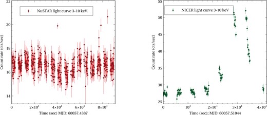
The left panel shows the NuSTAR light curve in the |$3-10$| keV energy band with 100 s binning. The right panel shows a similar light curve with NICER detector. A certain rise in the count rate (|$\sim 50$| cts s−1) is observed in the NICER light curve, which was absent during the NuSTAR observation.
