


ABSTRACT
Asteroids pose significant threats to Earth, necessitating early detection for potential deflection. Leveraging machine learning (ML), we classify asteroids into near-Earth Asteroids (particularly Atens, Amors, Apollos, and Apoheles) and non-near-Earth asteroids, further categorizing them based on hazard potential. Training the seven models on a comprehensive data set of 4687 asteroids, we achieve high accuracy in prediction. The predictive capability of these models is critical for informed decision-making in planetary defense strategies. We apply different regularization techniques to prevent overfitting and validate the models using a large unseen data set. A rigorous long-term N-body integration spanning 1 Myr is executed utilizing the Mercury N-body integrator to illuminate the evolution of asteroid properties over extended temporal scales. Following this integration process, the best-performing ML model is employed to classify asteroids based on their orbital characteristics and hazardous status respectively. Our findings highlight the effectiveness of ML in asteroid classification and prediction, paving the way for large-scale applications. By dividing a 1 Myr integration into intervals, we uncover temporal trends in asteroid behaviour, revealing insights into hazard evolution and ejection patterns. Notably, initially, hazardous asteroids tend to transition to non-hazardous states over time, elucidating key dynamics in planetary defense. We illustrate these findings through plotted graphs, providing valuable insights into asteroid dynamics. These insights are instrumental in advancing our understanding of long-term asteroid behaviour, with significant implications for future research and planetary protection efforts.
1 INTRODUCTION
Asteroids are rocky remnants originating from the early stages of our Solar system’s development and are commonly known as minor planets. They vary greatly in size, shape, and composition, ranging from small rocky bodies just a few meters in diameter to large, irregularly shaped objects spanning hundreds of kilometers. Most asteroids orbit the Sun within the asteroid belt, a region located between the orbits of Mars and Jupiter, although some travel on paths that bring them closer to Earth. While asteroids can be fascinating to study, they also pose a significant threat to life on Earth.
Over time, Earth has encountered many collisions with asteroids. For example, approximately 66 Myr ago, an asteroid estimated to be about 10 km in diameter struck what is now the Yucatán Peninsula in Mexico. This cataclysmic event, known as the Chicxulub impact (Morgan et al. 2022), is believed to have triggered one of Earth’s most significant mass extinction events, leading to the demise of the dinosaurs and numerous other species. Occurring approximately 35 Myr ago in what is now the Siberian region of Russia, the Popigai impact event (Bottomley et al. 1997) created one of the largest impact structures on Earth. The impact, caused by an asteroid or comet estimated to be several kilometers in diameter, resulted in the formation of a 100-km-wide crater. The Tunguska event (Longo 2007) occurred on the morning of 1908 June 30, when a bright, glowing object streaked across the sky and exploded with a force estimated to be equivalent to several megatons of TNT. The explosion released a shockwave that swept across the remote Siberian wilderness, flattening an estimated 80 million trees and causing widespread devastation. The 2013 Chelyabinsk meteor event (Yang et al. 2014), triggered by a relatively small asteroid, demonstrated the potential for significant damage and injuries from asteroid impacts. It underscored the importance of continued efforts in asteroid detection, monitoring, and mitigation to safeguard against future threats.
Asteroids categorized as near-Earth asteroids (NEAs) or Earth-approaching asteroids are those capable of traversing within the orbit of Mars. NEAs are specifically defined as asteroids with a perihelion distance (q) less than 1.3 au and an aphelion distance (Q) greater than 0.983 au (Bottke et al. 2000; Mako et al. 2005). NEAs can be classified into four categories based on geometric perspectives, which are Atens, Amors, Apollos, and Apoheles (Mako et al. 2005). Potentially hazardous asteroids (PHAs) are of particular concern due to their capability to pose a threat. PHAs encompass asteroids whose Earth Minimum Orbit Intersection Distance (MOID) measures 0.05 au or less, coupled with an absolute magnitude not exceeding 22 (Wie 2009). Asteroids that either maintain a minimum distance from Earth of 0.05 au (approximately 117 Earth radii) or possess a diameter smaller than roughly 150 m are excluded from the category of PHAs. To mitigate the potential threat from an asteroid, various authors have proposed different techniques depending on the warning time and the asteroid’s diameter to successfully deflect an asteroid. For instance, nuclear explosion device (Barrera 2004; Gennery 2004), Kinetic Impactors (Wie 2005; Sarli et al. 2017), gravity tractors (Lu & Love 2005), multiple gravitational tractors (McInnes 2007; Wie 2008), ion beam shepherd (Bombardelli & Peláez 2011; Bombardelli et al. 2013; Bombardelli, Amato & Cano 2016), etc. For choosing the best deflection method, warning time is crucial. Therefore, early detection is one of the critical factors in successfully deflecting an asteroid.
Due to the large number of asteroids inhabiting outer space and the extensive volume of data regarding their physical attributes and orbital paths, manual processing by humans is not feasible. ML stands out as an ideal choice for this task. Many authors have employed ML techniques for the classification of asteroids in the past. In their study, Mako et al. (2005) employed an artificial neural network (ANN) to classify asteroids into four distinct groups: Atens, Apollos, Amors, and Apoheles. Si (2020) in their research employed eight different ML techniques to classify potentially hazardous and non-hazardous asteroids.
The rest of the paper is structured as follows: Section 2 contains the data set and its pre-processing. In Section 3, we provide a brief overview of machine-learning methods. Section 4 discusses the long-term evaluation of asteroids. Sections 5 and 6 examine and discuss the outcomes produced by the most effective classifiers, along with temporal trends. Finally, Section 7 concludes our work.
2 DATA SET, ITS PRE-PROCESSING, AND GENERATING UNLABELLED DATA
This study applies ML algorithms to categorize asteroids based on their orbital characteristics into four groups: Atens, Apollos, Amors, and Apoheles. Then we focus on classifying asteroids into two groups: PHAs and potentially non-hazardous asteroids (PNHAs). The methodology involves training the algorithms on known asteroid data sets and then applying them to classify new asteroids into these pre-defined groups. Our selection of a renowned data set comprising 4687 observations is grounded in its widespread adoption by numerous researchers for model training and testing (Si 2020; Ramakrishnan 2021; Reddy et al. 2021). This data set encompasses diverse asteroids, featuring varying orbital characteristics, diameters, absolute magnitudes, MOID, and other pivotal attributes. Consequently, it is an optimal choice for our training set, offering robust representation across asteroid types.
We employed a random data set split into training and testing subsets, adhering to a conventional testing size of 20 per cent. Each asteroid entry in the data set comprises 40 features; however, not all are appropriate to classification criteria (e.g. close approach date, orbiting body, orbit determination date, name, equinox, etc.). These irrelevant features were consequently removed for both classification tasks. Subsequently, we constructed a correlation matrix for the remaining features, aiming to discard one of the two features if their correlation score exceeded –0.9 or 0.9. Despite this approach, it was observed that in a few cases, removing features based on high correlation led to decreased accuracy compared to models that retained features with correlation coefficients above –0.9 or 0.9. Consequently, we opted to include the following features for both classification tasks, namely absolute magnitude (H), MOID, semimajor axis (a), eccentricity (e), inclination (i), perihelion arg (|$\omega$|), ascending node longitude (|$\Omega$|), mean anomaly (M), perihelion distance (p), aphelion distance (Q), Jupiter Tisserand invariant, focal distance, and orbital period. Given that the computational expense of model training is manageable, incorporating these features does not adversely affect the study, provided accuracy is maintained and overfitting is avoided. In subsequent sections, we will explore the significance of these features in detail and assess whether any features should be prioritized.
In the first classification process for asteroids based on their orbital characteristics into NEAs (Atens, Amors, Apollos, and Apoheles) and non-NEAs groups, we begin by augmenting the data set with a new column. This column assigns one of the five groups to each asteroid utilizing the equations outlined in Mako et al. (2005). Subsequently, this new column is designated as the target for applying ML techniques. Our objective is to utilize our trained ML model for the classification of unseen data derived from numerically integrated trajectories projecting 1 Myr into the future. Specifically, we focus on the dynamic nature of asteroid trajectories, acknowledging the likelihood of certain asteroids transitioning within different groups of NEAs and also to non-NEAs after numerical propagation via the Mercury N-Body integrator (Chambers 1999). Given the absence of non-NEAs within our original data set, we implemented a strategic augmentation by introducing novel data points. These additional entries were systematically categorized within the non-NEAs classification, enriching the diversity and comprehensiveness of our data set. This augmentation is strategically aimed at fortifying the resilience and accuracy of our ML model in its capacity to effectively categorize unlabelled data sets in prospective scenarios. By accommodating potential alterations in asteroid attributes over time, our approach seeks to ensure the adaptability and reliability of the classification model in dynamic astronomical contexts. While Mako et al. (2005) employed a simple perceptron-like neural network for classification, we utilize various ML techniques and select the most effective one based on their evaluation metrics and their performance on unseen data sets. We train our model using both NEA and non-NEA asteroids to enhance its predictive power. After identifying the optimal model, we apply it to predict the classification of unseen data.
In the second classification task of asteroids into PHAs and PNHAs categories, we designate a specific column indicating whether an asteroid is hazardous as our target variable. However, due to the data set’s inherent imbalance – with approximately 84 per cent of asteroids classified as non-hazardous and only 16 per cent as hazardous – an ML model predicting all asteroids as non-hazardous would yield an accuracy of 84 per cent. Consequently, relying solely on accuracy for model evaluation becomes inadequate. In our data set, we encountered instances of duplicated asteroids with varying Epoch dates. As our classification task primarily focuses on distinguishing asteroids into two classes, these duplicates were deemed unnecessary for enhancing accuracy. Consequently, we systematically removed these redundant entries from our data set. Moreover, upon closer examination of the data set, we identified anomalies where certain asteroids were misclassified according to the definition of PHAs outlined in Wie (2008). Subsequently, we rectified these misclassifications, aligning them with the established criteria. This refinement notably improved the performance of various ML algorithms. Remarkably, even simpler models like decision trees demonstrated exceptional performance compared to more complex models applied to the original data set.
In our study, our primary focus lies in accurately classifying asteroids as potentially hazardous or non-hazardous. Considering the context, such as the medical field where falsely diagnosing a cancer patient as negative poses greater risks than diagnosing a non-cancer patient as positive, misclassifying a PHA as non-hazardous carries a higher potential cost compared to the reverse scenario. Therefore, it is essential to assess various evaluation metrics before determining the effectiveness of a model. Si (2020), Bahel et al. (2021), Ramakrishnan (2021), and Reddy et al. (2021) used various ML algorithms to classify PHAs and non-PHAs. An algorithm performing well on training and testing data can still fail to predict unseen data accurately. This phenomenon can occur due to several reasons, such as overfitting, data distribution shifts, or insufficient model generalization. The primary objective of this study is to identify the most effective model for predicting unseen data generated through long-term integration, and subsequently validate its accuracy. Once the optimal model is established, it will be applied on a large scale to conduct a comprehensive temporal analysis of asteroid behaviour.
3 MODEL EVALUATION AND ALGORITHM ANALYSIS
In this section, we investigate the critical aspects of evaluating ML models and analysing various algorithms. We begin with an overview of essential evaluation metrics that assess model performance. We also address model validation, including k-fold cross-validation and the use of external validation sets, to ensure model reliability. Next, we explore the role of hyperparameters and their tuning to optimize model accuracy. Additionally, we discuss the distinctions between parametric and non-parametric models, highlighting their respective advantages and use cases. Finally, we provide an in-depth analysis of several prominent ML techniques, such as ANN, K-nearest neighbours (KNN), decision trees, random forests (RF), extremely randomized trees (ExtraTree), Adaptive Boosting (AdaBoost), and Gradient Boosting (GBoost), examining their characteristics and application scenarios. In this work, we will apply these ML algorithms accessible in the scikit-learn package (Pedregosa et al. 2011).
3.1 Evaluation metrics
Evaluation metrics are important for assessing the performance of ML models. They offer quantitative insights into how effectively a model is handling a specific task. We’ll use metrics like accuracy, recall, precision, and F1 score to measure the model’s effectiveness. Accuracy measures the ratio of correctly identified instances to the total number of instances.
Precision measures the proportion of correctly identified positive predictions among all predicted positives, whereas recall evaluates the proportion of correctly identified positive predictions relative to all actual positive instances. In the second classification task, emphasis is placed on the recall score, reflecting the model’s capacity to accurately detect hazardous asteroids, thereby reducing false negatives and addressing the potential risks linked with overlooking hazardous entities. |$F1$| score balances precision and recall. These are given by
where |$T_{\text{Pos}}$| denotes the count of true positive instances (correctly predicted positive cases), |$F_{\text{Neg}}$| denotes the count of false negatives (incorrectly predicted negative cases), |$F_{\text{Pos}}$| denotes the count of false positives (incorrectly predicted positive cases). Then, we calculate
To calculate the average values of Precision, Recall, and F1 score, we employ both macro and weighted averages, depending on the classification task. The macro average method computes the evaluation metric separately for each class and then averages these scores. This approach treats each class equally, regardless of its frequency or any class imbalance in the data set. Conversely, the weighted-average method calculates the evaluation metric for each class and then computes the average, weighted by the support (the number of true instances) of each class. Detailed discussions on these methods are described in Hastie, Tibshirani & Friedman (2009) and Ivezić et al. (2020).
For the first classification problem, we use the weighted average due to our imbalanced data set. This method gives more weight to classes with larger support, providing a more representative overall evaluation of the model’s performance.
For the second classification problem, despite the data set’s imbalance, we use the macro-average method for computing evaluation metrics. As previously mentioned, there are fewer hazardous asteroids compared to non-hazardous ones. Misclassifying a hazardous asteroid as non-hazardous poses a greater threat than the reverse scenario. Using a weighted average, in this case, could allow poor performance in the hazardous group to be overshadowed by the larger non-hazardous group. However, this issue is less critical in the first classification task, as misclassifications within NEAs or between NEAs and non-NEAs are not as consequential.
In addition to the aforementioned metrics, we also employed the area under the precision-recall curve (AUC-PR) (Davis & Goadrich 2006) and the Matthews correlation coefficient (MCC) (Chicco & Jurman 2020). The AUC-PR is notably advantageous for unbalanced data sets, as it focuses on the model’s performance concerning the positive class, providing a comprehensive measure of the balance between precision and recall at varying thresholds. This metric is advantageous in scenarios where the positive class is of primary interest and is often used in binary classification. However, it can be extended to multiclass classification by averaging the precision-recall curves for each class.
The MCC is another robust metric for evaluating models on unbalanced data sets. It considers true and false positives and negatives, providing a balanced measure that can handle class imbalances effectively. The MCC is particularly suited for binary classification, but it can also be generalized to multiclass problems by calculating the coefficient for each class against all others and then averaging the results. MCC offers a more informative picture than accuracy, especially when working with data sets where one class is substantially underrepresented.
MCC is calculated as
The MCC score varies between –1 and +1, with +1 representing perfect classification and –1 indicating complete misclassification, and 0 represents a prediction no better than random chance.
AUC-PR and MCC are excellent evaluation metrics for unbalanced data sets, enhancing our ability to accurately assess model performance in binary and multiclass classification contexts. By employing these metrics alongside traditional measures, we ensure a comprehensive evaluation of our models’ predictive capabilities.
3.2 Model validation
We have already mentioned that we divided the data into 80 per cent for training and 20 per cent for testing. Although this initial separation helps in tuning model parameters for a particular data set, it does not ensure that the model will generalize well to other data sets. To validate the model’s reliability and ability to generalize, we employed k-fold cross-validation with k = 5. In k-fold cross-validation, the data set is divided into k equally sized folds. The model is trained using k – 1 of these segments and tested on the remaining segment. This procedure is performed k times, with each segment serving as the validation set once. For instance, with k = 5, the model is trained using the first four folds and evaluated on the fifth fold. This process is repeated until every fold has been utilized as the validation set, providing a thorough assessment of the model.
In addition to cross-validation, we addressed concerns of overfitting by evaluating the model’s performance on an external validation set comprising more than 35 000 unseen asteroids from the NASA JPL Solar System Dynamics database1 for each classification problem. This external validation set helped confirm the robustness and practical applicability of our models beyond the initial data set. Moreover, conventional evaluation metrics such as accuracy and F1 score, while valuable, may sometimes fail to fully reflect the model’s effectiveness on unknown data, potentially obscuring issues with generalization. By employing these comprehensive validation strategies, we aimed to demonstrate that our models are not only accurate but also capable of generalizing effectively to new, unseen data.
3.3 Hyperparamters and regularization
Hyperparameters, also known as free parameters, are settings or configurations that are independent of the model and cannot be derived from the training data. These parameters influence elements of the learning process, such as the model’s complexity and the behaviour of the learning algorithm. For instance, in the KNN algorithm, ‘k’ represents the number of neighbours to consider when making predictions. This hyperparameter significantly influences the model’s performance. Opting for a small ‘k’ value can result in overfitting, wherein the model excessively tailors itself to the training data, hampering its ability to adapt to new data. Conversely, selecting a large ‘k’ value may result in underfitting, causing the model to oversimplify the data and overlook its inherent patterns. In decision trees, hyperparameters like maximum tree depth, minimum samples required for splitting nodes, minimum samples needed for leaf nodes, and maximum features considered for each split are crucial. Using these parameters without appropriate limitations can lead to overfitting, as the model may become too complex and specifically adjusted to the training data, failing to generalize well to new data. Similarly, in the RF algorithm, the number of decision trees is a parameter we can adjust. Increasing the number of trees generally improves the model’s performance, but it also escalates the computational requirements. Since decision trees are used as a standalone component within RF, the hyperparameters of RF include those inherent to decision trees. These parameters profoundly impact the model’s behaviour and effectiveness, necessitating meticulous selection and tuning to optimize performance. We will employ GridSearchCV from the scikit-learn package to methodically investigate various configurations of hyperparameters and determine the optimal settings for our classification task.
Regularization techniques are employed to address the overfitting issue and facilitate effective generalization of the model to new, unseen data. Regularization is a technique that penalizes complex models by incorporating a regularization term into the loss function, which reduces excessive complexity and aids in preventing overfitting. For instance, in linear models, regularization terms like L1 (Schmidt, Fung & Rosales 2007) and L2 (Cortes, Mohri & Rostamizadeh 2012) penalties are used to constrain the magnitude of coefficients, thus simplifying the model. In decision trees and ensemble methods like Random Forests, regularization can be achieved by setting constraints on tree depth or the minimum number of samples required at a node, effectively controlling the growth of the trees and promoting generalization. Regularization helps maintain a trade-off between accurately fitting the training data and keeping the model simple enough to perform effectively on new, unseen data. By incorporating regularization techniques, we enhanced model robustness and predictive performance across various data sets. These techniques were specifically applied to address overfitting, as detailed in Sections 3.5–3.11.
3.4 ML Models: stand-alone, ensemble, and parametric versus non-parametric approaches
In our study, we employ both stand-alone and ensemble methods for classification. Stand-alone methods, such as ANN, KNN, and decision trees, utilize a single model to make predictions. In contrast, ensemble methods, such as RF, ExtraTrees, AdaBoost, and GBoost, combine multiple models to enhance predictive performance and robustness. Specifically, RF and ExtraTrees are bagging algorithms that create various instances of decision trees by training on different subsets of the data and then aggregating their predictions to improve accuracy and reduce overfitting. On the other hand, AdaBoost and Gradient Boost are boosting algorithms that sequentially train multiple weak learners, where each subsequent learner focuses on the errors made by its predecessors, thus improving the model’s overall performance. By integrating both bagging and boosting techniques, our study leverages the strengths of diverse ensemble methods to achieve superior classification results. More about these methods in detail can be found in Deitel & Deitel (2022), Alpaydin (2020), and Swamynathan (2017).
In ML, both parametric and non-parametric methods are utilized for estimation and modelling, much like their counterparts in statistics. Parametric estimation involves defining a model across the complete input space and acquiring its parameters by utilizing all accessible training data. In contrast, non-parametric estimation encompasses segmenting the input space into localized regions, typically delineated by a distance metric like the Euclidean norm. The respective local model, derived from the training data within that particular region, is applied to each input. This approach allows for more flexible and adaptive modelling, particularly in scenarios where the underlying data distribution may be complex or heterogeneous
3.5 Artificial neural network
The architecture diagram in Fig. 1 outlines the fundamental structure of an ANN. It encompasses an input layer, a hidden layer, and an output layer. The input layer receives three distinct inputs, which are processed and passed on to the hidden layer. The hidden layer is composed of two neurons that perform computations on the weighted sum of the inputs, applying an activation function to produce an intermediate output. This intermediate output is then fed into the output layer, which generates the network’s final output. This simple architecture illustrates the fundamental components of a neural network, showcasing the flow of information from inputs through a processing unit to an output, essential for tasks such as classification and regression in ML applications. More details of ANN can be found in Hassoun (1995) and Yegnanarayana (2009).
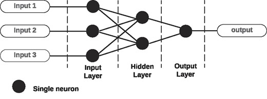
ANN architecture.
An MLP classifier, short for multilayer perceptron, represents a specific type of ANN employed predominantly for classification purposes. It incorporates numerous layers of neurons, encompassing an input layer, one or more hidden layers, and an output layer. Renowned for their adaptability, MLPs excel in discerning intricate patterns within data sets, rendering them invaluable across diverse ML applications. However, the capacity of MLPs to model complex patterns also makes them susceptible to overfitting. Therefore, we employ L2 regularization, which penalizes large weights to mitigate model complexity, and early stopping, which halts training when performance ceases to improve on a validation set. To ensure effective learning, maximum number of iterations is set to 1000, allowing the model sufficient epochs to converge. These techniques collectively help in achieving a balanced model that generalizes well to new, unseen data while avoiding the pitfalls of overfitting. Further optimizing the performance of the MLP classifier involves tuning several hyperparameters that directly impact the model’s learning dynamics and capacity. For our study, we conduct a grid search over the following hyperparameters:
(i) hidden_layer_sizes: specifies the number of neurons in each hidden layer;
(ii) alpha: the L2 regularization parameter governs the intensity of regularization applied to the model’s weights;
(iii) learning_rate_init: the initial learning rate influences the size of weight updates during training; and
(iv) activation: the choice of activation function, either relu or tanh, affects how neurons process and transmit information.
We performed an extensive hyperparameter search by varying the following parameters to identify the optimal configuration for both the classification problem: hidden_layer_sizes: [50, 100, 150], alpha: [0.0001, 0.001, 0.01], learning_rate_init: [0.001, 0.01, 0.1], and activation: [relu, tanh]. After fitting the model with five-fold cross-validation across these 54 candidates, we determined the best hyperparameters to be hidden_layer_sizes = 100, alpha = 0.0001, learning_rate_init = 0.01, and activation = tanh. This configuration yielded a weighted average F1 score of 0.9770 and an MCC of 0.9643. For categorizing asteroids as either hazardous or non-hazardous, the optimal hyperparameter values were identified as hidden_layer_sizes = 50, alpha = 0.01, learning_rate_init = 0.1, and activation = relu. This resulted in a macro average F1 score of 0.9705 and MCC of 0.9414.
The MLP model, following an extensive hyperparameter search and cross-validation, exhibited robust performance, achieving high F1 scores and MCC values, underscoring its effectiveness in accurately classifying the asteroid data.
3.6 K-nearest neighbour
KNN is one of the simplest classification algorithms supported by the scikit-learn package. It’s deemed a non-parametric technique due to its lack of assumptions regarding the inherent data distribution. The algorithm memorizes the training data throughout the training process without imposing pre-defined parameters. There is no explicit training step like in many other ML algorithms. More about the theory of the KNN method can be found in Peterson (2009) and Kramer (2013).
The KNN algorithm, illustrated in Fig. 2, represents the classification process within a two-dimensional feature space containing labelled categories: Category A, Category B, and Category C. The data point to be classified is depicted by a black dot within this space. The algorithm determines the nearest neighbours to the black dot using a distance metric, typically Euclidean distance. In this example, the neighbours are denoted by points within the feature space corresponding to different categories. The majority category among these neighbours determines the classification of the point. In KNN, k is a hyperparameter. If we choose k = 5, the model will select the five nearest neighbours to the point and vote. The category with the majority ‘votes’ will determine the classification. The KNN algorithm is a simple yet powerful instance-based learning method that classifies data points based on the most common category among their closest neighbours. In addition to k, the following hyperparameters were also explored to optimize model performance:

KNN architecture.
(i) weights: determines how the contribution of each neighbour is weighted;
(ii) algorithm: specifies the method used to calculate the nearest neighbours; and
(iii) p: the power parameter for the Minkowski distance metric.
We have varied the following hyperparameters for the KNN classification: k: [3, 5, 7, 9, 11], weights: [uniform, distance], algorithm: [ball_tree, kd_tree, brute], and p: [1, 2, 3, 4]. After testing these variations, we identified the best hyperparameters for the first classification problem as k = 11, weights = distance, algorithm = ball_tree, and p = 1 (equivalent to Manhattan distance). These settings resulted in weighted average F1 score of 0.9262 and MCC of 0.8854.
For the classification into hazardous and non-hazardous, we obtained the optimal value of hyperparameters as k = 7, weights = distance, algorithm = ball_tree, and p = 1 with macro average F1 score of 0.7910 and MCC of 0.6048. Performance of KNN was relatively low when compared with other models.
3.7 Decision tree
The decision tree diagram in Fig. 3 illustrates the hierarchical structure used in decision tree classification and regression models. Quinlan (1986) introduced this classification algorithm. At the top of the tree is the root node, which represents the initial decision point based on a specific feature. From the root node, branches lead to decision nodes, where further decisions are made based on additional features. These decision nodes further branch out until they reach leaf nodes, which represent the outcome or class label. Each path from the root node to a leaf node represents a series of decisions leading to a specific classification or prediction. The diagram highlights how decision trees partition the feature space into regions associated with different outcomes, enabling clear, and interpretable decision-making processes. As previously mentioned, tuning the hyperparameters of a decision tree classifier is essential for optimizing model performance and potentially helping our model to not become overly complex, thus preventing overfitting. For our study, we have employed a grid search over these parameters:
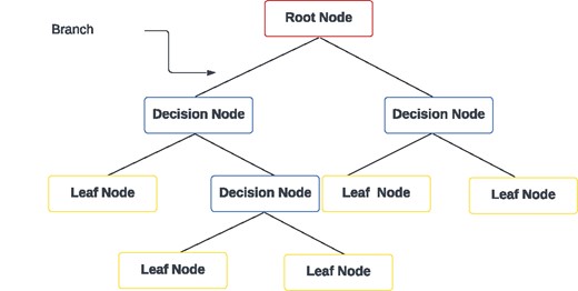
Decision tree.
(i) criterion: function used to measure the quality of a split;
(ii) max_depth: controls the maximum depth of the tree;
(iii) min_samples_split: minimum number of samples required for splitting an internal node;
(iv) min_samples_leaf: the smallest number of samples needed to form a leaf node;
(v) ccp_alpha: controls the complexity for minimal cost-complexity pruning; and
(vi) class_weight: weights associated with classes to handle class imbalance.
We have varied the following hyperparameters for the classification problems: criterion: [gini, entropy, log_loss], max_depth: [5, 10, 15], min_samples_split: [5, 10, 20], min_samples_leaf: [2, 5, 10], ccp_alpha: [0.01, 0.1, 1.0], and class_weight = [None, balanced]. After testing these variations, we identified the best hyperparameters as: criterion = gini, max_depth = 5, min_samples_split = 5, min_samples_leaf = 2, ccp_alpha = 0.01, and class_weight = None. This configuration resulted in a weighted average F1 score of 0.9990 and MCC of 0.9984. With varying the same hyperparameters for the second classification, the optimal hyperparameters identified were: criterion = gini, max_depth = 5, min_samples_split = 5, min_samples_leaf = 2, ccp_alpha = 0.01, and class_weight = None. This set up resulted in macro average F1 score of 0.9974 and MCC of 0.9948.
The decision tree model achieved exceptional performance across both classification tasks, with optimal hyperparameters consistently resulting in very high F1 scores and MCC. Its configuration demonstrated strong predictive accuracy and robustness, confirming its efficacy for the classification problems addressed.
3.8 Random forest
RF, a prominent ensemble learning method that was introduced by Breiman (2001), has attracted significant attention across various domains for its robustness and predictive accuracy. It functions by combining the outputs of multiple decision trees, each trained on different portions of the training data. These decision trees, which form the core components of an RF, are hierarchical structures where each node signifies a feature and each branch indicates a decision based on that feature. RF chooses the best split among features at each node, optimizing for predictive performance. This ensemble technique harnesses the power of combining diverse decision trees to mitigate overfitting and improve generalization performance. Moreover, RF introduces randomness at two key stages: during the bootstrap sampling of training data and the selection of features for each tree’s decision-making process. A key hyperparameter is the ‘number of estimators’, which specifies the number of individual decision trees in the forest. This parameter is crucial as it influences the model’s complexity and predictive performance. Through meticulous tuning of hyperparameters such as the number of estimators and those specific to decision trees, RF offers a versatile and effective approach for classification and regression tasks, making it a staple in ML practice.
We have varied the following hyperparameters for both the classifications: n_estimators: [50, 100, 200], criterion: [gini, entropy, log_loss], max_depth: [5, 10, 15], min_samples_split: [2, 5, 10], min_samples_leaf: [1, 2, 4], bootstrap: [True, False], and class_weight: [None, balanced]. After testing these variations, we identified the best hyperparameters for the first classification problem as n_estimators = 100, criterion = gini, max_depth = 10, min_samples_split = 2, min_samples_leaf = 1, bootstrap = True, and class_weight = None, achieving a weighted average F1 score of 0.9990 and MCC of 0.9984. For the second classification, the optimal values of the hyperparameters were as follows: n_estimators = 50, criterion = gini, max_depth = 10, min_samples_split = 2, min_samples_leaf = 1, bootstrap = True, and class_weight = None. It yielded a macro average F1 score of 0.9974 and MCC of 0.9948.
The optimal hyperparameters consistently delivered very high F1 scores and MCCs, demonstrating the model’s robustness and accuracy in handling the classification problems.
3.9 Extremely randomized trees
ExtraTrees, also known as extremely randomized trees, is an ensemble learning approach akin to RFs (Geurts, Ernst & Wehenkel 2006). It builds multiple decision trees during training and combines their outputs to generate predictions. However, ExtraTrees introduces additional randomness in the tree construction process. Unlike RF, which selects the best split among a subset of features, ExtraTrees randomly selects splits for each feature at every node. This heightened level of randomness can lead to faster training times since it eliminates the need to find the optimal split. Additionally, the randomness introduced in ExtraTrees helps to further diversify the ensemble, making it less prone to overfitting. Despite its increased computational efficiency, ExtraTrees typically requires more trees in the ensemble to achieve comparable performance to RF. The number of estimators, as in RF, remains a crucial hyperparameter in tuning the performance of ExtraTrees. Overall, ExtraTrees offers a compelling alternative to RF, particularly in scenarios where computational resources are limited or when dealing with high-dimensional data.
We varied the same set of hyperparameters for ExtraTrees as we did for RF, fine-tuning the model to achieve optimal performance. For the first classification task, we identified the optimal value of the hyperparameters as n_estimators = 200, criterion = entropy, max_depth = 15, min_samples_split = 2, min_samples_leaf = 1, bootstrap = False, and class_weight = None. This configuration yielded a weighted average F1 score of 0.9863 and an MCC of 0.9789. For the second classification, we obtained the optimal value of the hyperparameters to be n_estimators = 200, criterion = gini, max_depth = 15, min_samples_split = 5, min_samples_leaf = 1, bootstrap = True, and class_weight = balanced, resulting in a macro average F1 score of 0.9474 and MCC of 0.8947.
The ExtraTree model demonstrated strong performance for both classification tasks, with particularly high results in the first classification problem.
3.10 Adaptive boosting
AdaBoost is an influential ensemble technique that enhances the performance of multiple weak learners, such as decision trees, to build a more robust classifier (Zhou 2012). Unlike bagging methods, AdaBoost emphasizes misclassified instances by increasing their weights, thereby focusing subsequent classifiers on these harder cases. Initially, all data points and classifiers are assigned equal weights. As the training progresses, classifiers that misclassify instances are adjusted by increasing the weights of those particular data points. Consequently, these misclassified data points exert a greater influence on the model in the next iteration. This process repeats, iteratively refining the model until it either achieves a satisfactory level of accuracy or reaches the maximum number of specified estimators. The method culminates in a final prediction obtained through a weighted average of all individual classifiers. A pivotal hyperparameter in AdaBoost is the ‘number of estimators’, which has been optimized using GridSearchCV to identify the optimal value within specified values: [50, 100, 200]. Additionally, hyperparameters such as maximum depth and learning rate play a critical role in the model’s performance and are essential for preventing overfitting. For these hyperparameters, we varied the values within a restricted range: [1, 2, 3] for max_depth and [0.01, 0.1, 1] for learning rate. The choice of these relatively small values results in simpler, less complex weak learners, thereby mitigating the risk of overfitting and enhancing the model’s generalizability.
For the first classification problem, we identified the best combination of hyperparameters as n_estimators = 200, max_depth = 2, and learning_rate = 0.01. This configuration yielded a weighted average F1 score of 0.9990 and a MCC of 0.9984. In the subsequent classification task, the optimal values of the hyperparameters are given by n_estimators = 50, max_depth = 1, and learning_rate = 0.1. This configuration resulted in macro average F1 score of 0.9974 and MCC of 0.9948.
The AdaBoost classifier achieved exceptional results in both classification tasks, with optimal hyperparameter configurations delivering excellent performance metrics.
3.11 Gradient boosting
Gboost is a potent ensemble method that constructs a resilient model by progressively incorporating weak learners, often in the form of decision trees (Schapire & Freund 2013; Swamynathan 2017). Unlike AdaBoost, which adjusts the weights of misclassified instances, Gboost focuses on minimizing the residual errors of previous models. Each new learner is trained to correct the mistakes of their predecessors by fitting them to the residual errors, effectively reducing the overall error of the model. This iterative process continues until a pre-defined number of learners is reached or the error is sufficiently minimized. A crucial aspect of Gboost is its learning rate, a hyperparameter that determines the contribution of each learner to the final model. Additionally, the number of estimators, which indicates the number of weak learners to be combined, is another vital parameter. The max_depth of each tree is also a key hyperparameter, influencing the complexity of the model and its ability to capture complicated data patterns. These hyperparameters are often tuned using techniques like GridSearchCV to optimize model performance. We adjusted the same set of hyperparameters for Gboost as we did for AdaBoost. Gboost’s ability to handle complex patterns and interactions within the data makes it a preferred choice for various ML tasks.
In our first classification task, we used |$GridSearchCV$| to find the optimal value of the hyperparameters, which were determined to be n_estimators = 50, max_depth = 3, and learning_rate = 0.01. This configuration produced a weighted average F1 score of 0.9990 and an MCC of 0.9984. In the second classification task, the optimal hyperparameter configuration: n_estimators = 50, max_depth = 3, and learning_rate = 0.01, resulted in a macro average F1 score of 0.9974 and an MCC of 0.9948.
The GBoost classifier achieved outstanding results in both classification tasks, with impressive performance metrics attained through the optimal hyperparameter configurations.
4 EVOLUTION OF ASTEROIDS
In this section, we explore the long-term evolution of asteroids, emphasizing the simulation of their dynamical behaviour with high accuracy. We used symplectic integrators which are numerical algorithms designed for accurately simulating Hamiltonian systems by preserving the symplectic structure of phase space, ensuring long-term stability and energy conservation (Yoshida 1990; Sanz-Serna 1992; Duncan, Levison & Lee 1998). Particularly advantageous in scenarios dominated by a single massive body, such as planetary systems, these integrators leverage symplectic geometry to maintain long-term stability and conserve phase-space volume. By decomposing the Hamiltonian into kinetic and potential energy components, they advance the system’s dynamical variables through discrete time steps while ensuring symplectic behaviour, typically via explicit or implicit numerical schemes.
Understanding the principles of symplectic integrators begins with Hamilton’s equations of motion, which dictate the changes in position (x) and momentum (p) for each object within an N-body system:
Here, the Hamiltonian (H) represents the total energy of the system, combined kinetic and potential energies for all bodies:
In this equation, |$m_{i}$| represents the mass of body i, and |$r_{ij}$| denotes the separation between bodies i and j.
Symplectic integrators (Chambers 1999) operate by decomposing the Hamiltonian into manageable components, allowing for an approximate but efficient simulation of complex systems. The key insight lies in the non-commutativity of the operators associated with each component of the Hamiltonian. By sequentially applying these operators, the integrator can accurately approximate the time evolution of the system’s variables while preserving important physical properties. A critical step in their construction involves carefully choosing how to split the Hamiltonian into dominant and perturbative components, which helps optimize computational efficiency. By splitting the Hamiltonian in this manner, the integrator accurately models the system while avoiding excessive computational effort. Historically, these integrators have faced challenges, particularly with problems involving close encounters and small bodies on planet-crossing orbits within the Solar system.
In addressing close encounters within symplectic integrators, several critical assumptions, and strategies are employed to maintain the accuracy and stability of the integration. One primary assumption is that the Hamiltonian can be splitted into components, |$H_{A}$| and |$H_{B}$|, where |$H_{A}$| represents the dominant part, typically involving Keplerian motion around the Sun, and |$H_{B}$| represents perturbative interactions between bodies. During a close encounter, the separation between bodies becomes very small, causing a term in |$H_{B}$| to increase significantly. This increase in |$H_{B}$| can cause the error per integration step to rise dramatically from |$O(\varepsilon t^{3})$| to |$O(t^{3})$|, potentially destabilizing the simulation. To mitigate this, the term involving the close encounter is transferred from |$H_{B}$| to |$H_{A}$|, ensuring that |$H_{A}$| remains analytically integrable. This transfer allows for the accurate numerical integration of the close encounter terms while preserving the symplectic nature of the integrator. Additionally, mixed-centre coordinates (heliocentric coordinates and barycentric velocities) are assumed, as they simplify the integration process during close encounters compared to Jacobi coordinates. This approach ensures that the Hamiltonian terms are handled in a way that minimizes computational errors and maintains the integrator’s long-term stability and accuracy, even in the presence of frequent and significant close encounters.
To simplify the calculations and reduce computational burden, collisions and fragmentation of bodies are avoided during simulations. Planetary embryos are treated as point masses and instead of directly modelling collisions, a gravitational smoothing length of |$\delta$| = |$3 \times 10^{-8}$| au (approximately 5 km) is used. This smoothing length modifies the gravitational force between two bodies by replacing the usual expression with a softened version:
This softened force reduces the strength of gravitational interactions when two bodies are very close to each other, preventing the force from becoming infinitely large and causing numerical instabilities.
The Mercury N-body integrator, a computational tool commonly employed in astrodynamics, incorporates symplectic integration techniques to simulate gravitational interactions among multiple celestial bodies, particularly within complex planetary systems like our own (Chambers 1999). Utilizing numerical methods, it accurately calculates the trajectories of these bodies, enabling scientists to predict their positions and movements with precision. Long-term integration, a fundamental aspect of this computational approach, plays a crucial role in astronomical research by facilitating the detailed examination of planetary system dynamics over extended temporal scales. Long-term integration proves invaluable in assessing the potential hazard posed by asteroids. By simulating asteroid trajectories over millennia, researchers can identify potential impact risks and develop strategies for planetary defense.
We used the Mercury N-body integrator to simulate the long-term orbital evolution of asteroids in the Solar system, with the Sun positioned at the centre. Perturbations from all eight planets and Pluto were considered to ensure comprehensive gravitational interactions. We performed two integrations: one that included non-gravitational perturbations – such as the Yarkovsky effect, solar radiation pressure, and thermal forces – and one that excluded these factors. Given that the magnitude of these non-gravitational perturbations, ranging from |$10^{-12}$| to |$10^{-15}$|, was significantly smaller compared to the gravitational perturbations, no discernible changes in the results were observed throughout the 1 Myr of numerical integration. Fig. 4 shows that the numerical simulations produced by the symplectic integrator accurately reflect the behaviour of the underlying Hamiltonian system. It shows the energy error plot for both integrations, with both lines intersecting at all points across the 1 Myr range. This indicates that the conservation of energy remained consistent for both processes, further supporting the negligible impact of the non-gravitational forces within this timeframe. This is reliable data for us since energy is being conserved to a high degree of accuracy.
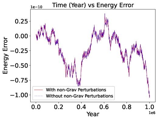
Time versus energy error graph illustrating the performance of the simulation over a 1 Myr period.
The starting epoch for the planets was set at 2457724.5 Julian days. The epochs of the integrated asteroids varied from 2450164.5 to 2458019.5 Julian days. At the beginning of the integration, the integrator synchronizes the epochs of both the perturbing planets and the asteroids.
The orbital elements of the asteroids were input as Keplerian Orbital Elements: a, e, i, w, |$\Omega$|, and M. For the integration process, we selected the Bulirsch–Stoer (BS) integrator due to its high accuracy, particularly in scenarios where other integrators might fail or need validation. Despite being slower, the BS integrator is reliable for precise simulations.
Parameters that were set for the integration process are shown in Table 1. In the integration process, specific settings were applied to manage close encounters. Integration was not halted after close encounters, ensuring continuous analysis without interruptions. The time was expressed in years for ease of interpretation, and it was not adjusted relative to the integration start time, providing a consistent temporal framework throughout the simulation. These settings were chosen to maintain a clear and straightforward analysis of the asteroid orbits over the long-term integration period.
Parameters used for the long-term integration of the asteroids.
| Parameter | Value |
|---|---|
| Starting time in days | 2458400.5 JD |
| Stopping time in days | 367701640.5 JD |
| Interval of output in days | 365 200.5 |
| Timestep in days | 8 |
| Parameter of accuracy | |$10^{-12}$| |
| Precision of output | High |
| Distance for ejection in au | 100 |
| Central body’s radius in au | 0.005 |
| Central mass (Solar) | 1.0d0 |
| Hill radii | 3.0 |
| Number of time steps between data dumps | 5000 |
| Number of time steps between periodic effects | 100 |
5 NEAs AND NON-NEAs IDENTIFICATION
Initially, utilizing the previously mentioned ML algorithms, asteroids are classified based on their orbital characteristics into distinct groups: Atens, Amors, Apollos, Apoheles, and non-NEAs. Here, the first four groups are NEAs. The performance evaluation of our models is presented in Table 2.
Below is the evaluation matrix of each ML algorithm used for the classification based on orbital characteristics (weighted avg).
| Models | Accuracy | Precision | Recall | F1 | MCC | False prediction |
|---|---|---|---|---|---|---|
| MLP | 0.9773 | 0.9772 | 0.9773 | 0.9770 | 0.9643 | 963 |
| KNN | 0.9279 | 0.9289 | 0.9279 | 0.9262 | 0.8854 | 4754 |
| DT | 0.9990 | 0.9990 | 0.9990 | 0.9990 | 0.9984 | 14 |
| RF | 0.9990 | 0.9991 | 0.9990 | 0.9990 | 0.9984 | 19 |
| ExtraTree | 0.9866 | 0.9867 | 0.9866 | 0.9863 | 0.9789 | 899 |
| Adaboost | 0.9990 | 0.9990 | 0.9990 | 0.9990 | 0.9984 | 14 |
| Gboost | 0.9990 | 0.9990 | 0.9990 | 0.9990 | 0.9984 | 14 |
Mako et al. (2005) demonstrated that the semimajor axis and focal distance are the features that enable linear separability among different groups. Utilizing only these two features resulted in good accuracy across all models. Different combinations of features that include the semimajor axis and focal distance consistently yielded high accuracy and performance on unseen data. Despite this, we opted to use all the features as earlier mentioned for the classification problem, as this approach achieved exceptional performance on the unseen data, with only fourteen errors out of more than 35 000 instances for the best-performing model. Decision tree, AdaBoost, and Gboost performed best among the seven models we evaluated. We selected the decision tree model for its superior efficiency, as it demonstrated the fastest training time, making it the most time-efficient option. Consequently, we employed the decision tree algorithm to classify unseen data.
The AUC-PR curve for decision tree in Fig. 5 shows that the model performs exceptionally well, achieving high precision and recall for all classes. Specifically, classes with an AUC-PR of 1.0000, such as Apoholes, Aten, and non-NEAs, indicate that the model distinguishes these classes perfectly from others. For the Apollo and Amor classes, the AUC-PR values of 0.9990 and 0.9951, respectively, still reflect excellent performance with only minimal deviations from perfect precision and recall. Overall, the AUC-PR curve demonstrates that the model maintains high precision and recall across all classes, indicating strong overall performance.
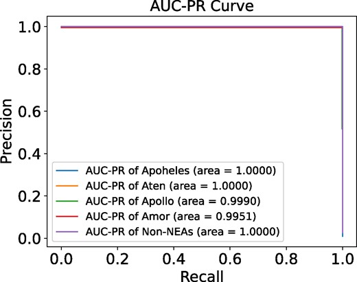
AUC-PR curve for decision tree classification of NEAs and non-NEAs, showcasing the model’s precision-recall performance.
Following Carruba et al. (2020), the primary objective of a classification algorithm is to identify new members within designated groups. Our model can accurately classify data sets from various sources such as JPL Horizons, Minor Planet Center, and the Asteroid Family Portal. However, our interest extends beyond present-day classification; we aimed to forecast the trajectories of asteroids 1 Myr into the future to gain insights into the evolutionary dynamics of our Solar system. Upon applying our model to the data set, notable observations emerged: Many asteroids initially categorized as NEAs were no longer classified as such after the 1 Myr projection. Table 3 presents the predictions derived from our model.
Classification of 1663 asteroids after 1 Myr as predicted by our model.
| Groups | Initially | After 1 Myr | Ejected asteroids |
|---|---|---|---|
| Atens | 245 | 219 | 0 |
| Amors | 440 | 300 | 42 |
| Apollos | 971 | 839 | 116 |
| Apoheles | 7 | 33 | 0 |
| Non-NEAs | 0 | 114 | 0 |
| Groups | Initially | After 1 Myr | Ejected asteroids |
|---|---|---|---|
| Atens | 245 | 219 | 0 |
| Amors | 440 | 300 | 42 |
| Apollos | 971 | 839 | 116 |
| Apoheles | 7 | 33 | 0 |
| Non-NEAs | 0 | 114 | 0 |
After a million year, we observed that asteroids belonging to neither the Atens nor Apoheles groups were ejected, but approximately 9.55 per cent of Amors and 11.95 per cent of Apollos were ejected from the Solar system. Although there were no non-NEAs at the beginning of the integration, many NEAs migrated to the non-NEAs group over time. The data further reveal that Atens, Amors, and Apollos experienced a moderate to significant decline in their populations, while Apoheles and NEAs exhibited an increase in their numbers over the same period. These observations underscore the dynamic nature of asteroid trajectories and the potential for significant changes in their classification over extended periods.
The provided line plot in Fig. 6 illustrates the transitions of asteroids among different groups – Apoheles, Atens, Apollos, Amors, and non-NEAs – over 1 Myr, segmented into 100 000-yr intervals. The first graph focuses on asteroids that were initially non-hazardous, while the second graph pertains to initially hazardous asteroids.
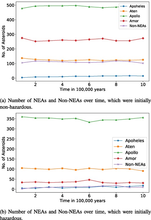
Number of asteroids belonging to NEAs (Apoheles, Aten, Apollos, and Amors) and non-NEAs over time.
For, initially non-hazardous asteroids, the Apollo group shows the highest stability and population, maintaining numbers between 478 and 498. This indicates a dominant and resilient nature. The Amors group, which starts with 275 asteroids, the group exhibits moderate stability with fluctuations around a relatively stable range over time, varying between 252 and 275, suggesting dynamic transitions possibly due to changing orbits or interactions. The Atens maintain a stable population, fluctuating slightly between 120 and 137, similar to their initially hazardous counterparts. The non-NEAs exhibit an increase from 102 to 118, with slight fluctuations, indicating moderate stability. The Apoheles group is the smallest and displays a general upward trend with increasing numbers over time, ranging from 4 to 16, indicating a growing population.
Conversely, the Apollo group remains the most populous for initially hazardous asteroids, with numbers fluctuating between 333 and 360. This suggests a stable orbital nature, with minimal transitions into or out of the group. The Atens maintain a fairly constant count, ranging from 91 to 105, indicating a stable behaviour similar to the Apollos. The Amors group, while stable, demonstrates slight fluctuations in their numbers, ranging from 30 to 47. Non-NEAs show a gradual increase from 2 to 19, indicating a slight but steady transition over time. The Apoheles group shows a fluctuating trend with a notable increase in numbers over time, ranging from 5 to 18, indicating both variability and growth in population. Overall, the Apollo group remains the most stable and dominant, while the other groups show moderate stability with slight increases or decreases over the period.
Additionally, the percentage of non-NEAs is notably higher in the case of initially non-hazardous asteroids compared to initially hazardous asteroids throughout the period. In initially hazardous asteroids, the number of Atens consistently exceeds the number of Amors. Conversely, in the case of initially non-hazardous asteroids, the number of Amors is consistently greater than that of the Atens throughout the time interval. This indicates differing evolutionary dynamics and stability between these groups depending on their initial hazardous status.
Overall, the Apollo group remains the largest and most stable across both initially hazardous and non-hazardous asteroids, highlighting their dominant and resilient nature. The Atens also show stability, while the Amors exhibit more dynamic changes, especially among initially non-hazardous asteroids. Non-NEAs maintain moderate stability in both cases, and the Apoheles remain the least numerous and stable for most of the instances. These observations suggest that Apollos and Atens have more stable long-term dynamics, while Amors and non-NEAs are more susceptible to changes over extended periods.
6 POTENTIALLY HAZARDOUS AND NON-HAZARDOUS IDENTIFICATION
Our primary focus lies in distinguishing between PHAs and PNHAs. We employed the same ML models in the previous classification task to achieve this. These models were trained to differentiate between asteroids with the potential to pose a hazard to Earth and those deemed non-hazardous. The performance evaluation of our models is presented in Table 4.
Below is the evaluation matrix of each ML algorithm used for the classification based on hazardousness.
| Models | Accuracy | Precision | Recall | F1 | MCC | False prediction |
|---|---|---|---|---|---|---|
| MLP | 0.9851 | 0.9796 | 0.9619 | 0.9705 | 0.9414 | 382 |
| KNN | 0.9091 | 0.8679 | 0.7485 | 0.7910 | 0.6048 | 1615 |
| DT | 0.9986 | 0.9956 | 0.9992 | 0.9974 | 0.9948 | 16 |
| RF | 0.9986 | 0.9956 | 0.9992 | 0.9974 | 0.9948 | 25 |
| ExtraTree | 0.9729 | 0.9474 | 0.9474 | 0.9474 | 0.8947 | 480 |
| AdaBoost | 0.9986 | 0.9956 | 0.9992 | 0.9974 | 0.9948 | 16 |
| Gboost | 0.9986 | 0.9956 | 0.9992 | 0.9974 | 0.9948 | 16 |
This suggests that decision tree, AdaBoost, and Gboost are the most reliable ML models for predicting unseen data, based on evaluation metrics for predicting whether an asteroid is hazardous or non-hazardous. Therefore, we will initially apply all three models to predict unseen data obtained after half a million years and a million years. If their predictions align, we will adopt the decision tree model for its simplicity, computational efficiency, and effectiveness, ensuring a streamlined approach without sacrificing generalizability. Table 5 reveals notable transitions between hazardous and non-hazardous asteroids. During model training, key features such as MOID and Absolute Magnitude (H) emerged as crucial determinants. Remarkably, the models’ performance, as reflected in evaluation metrics and results on unseen data, was equally excellent whether using only these two features or incorporating all the earlier mentioned features. This finding suggests that MOID and absolute magnitude alone are sufficient for achieving high accuracy in predictions. As the false prediction of PHAs and PNHAs can have severe consequences, we recognize the limitations of solely relying on evaluation metrics. Although a model might achieve strong performance on training and testing data, its effectiveness in accurately predicting unseen data remains uncertain. So, we conducted a comprehensive investigation into the predictive capabilities of our model.
Classification of 1663 asteroids after 1 Myr as predicted by our model.
| Groups | Initially | After 1 Myr | Ejected asteroids |
|---|---|---|---|
| Hazardous | 569 | 402 | 63 |
| Non-hazardous | 1094 | 1103 | 95 |
| Groups | Initially | After 1 Myr | Ejected asteroids |
|---|---|---|---|
| Hazardous | 569 | 402 | 63 |
| Non-hazardous | 1094 | 1103 | 95 |
The AUC-PR curve for the binary classification of hazardous and non-hazardous asteroids, as depicted in Fig. 8, indicates that the model exhibits near-perfect performance. The AUC-PR value of 0.9999 demonstrates that the model achieves extremely high precision and recall, with minimal trade-offs between these metrics. The curve remains almost flat at the top, indicating that the model maintains high precision even as recall increases. This suggests that the model is highly effective at differentiating between hazardous and non-hazardous asteroids, thereby reinforcing its robustness and reliability in this classification task.
Comparative analysis of hazardous asteroid prediction over time with known hazardous asteroids: evaluating model performance across time intervals.
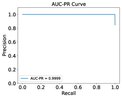
AUC-PR curve for decision tree classification of PHAs and PNHAs, highlighting the model’s precision-recall performance.
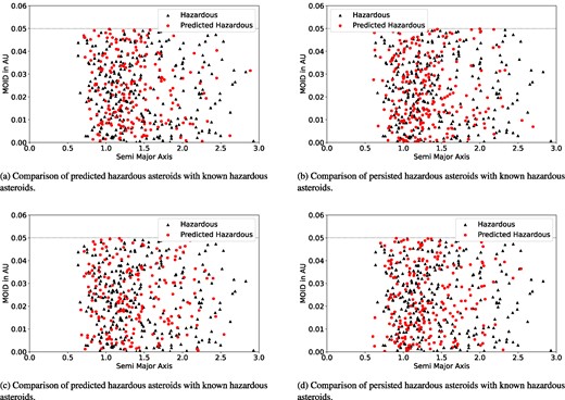
Before applying our best-performing models, decision tree, AdaBoost, or Gboost on a large scale, it is essential to validate the credibility and robustness of their predictive power. In our long-term integration process, we specifically selected asteroids with an estimated minimum diameter [Est Dia in KM (min)] equal to or greater than 0.150 km, as these asteroids have the potential to pose a significant threat. Furthermore, a notable observation is that all these asteroids exhibit an Absolute Magnitude value less than or equal to 22. Therefore, in determining whether an asteroid is hazardous, a crucial criterion is its MOID value. Given the substantial risks associated with misclassifying an asteroid as hazardous or non-hazardous, we meticulously assess the accuracy of both predictions to ensure the reliability and safety of our model’s predictions.
We present Fig. 7, which projects the semimajor axis (a) against the MOID value. The left panel compares initially non-hazardous asteroids that were predicted as hazardous (red dots) by the decision tree model after half a million and 1 Myr, respectively, against known hazardous asteroids (black triangles). The right panel contrasts initially hazardous asteroids that persisted as hazardous (red dots) according to the decision tree model after half a million and 1 Myr, respectively, with known hazardous asteroids (black triangles).
The cohesive clustering of red circles and black triangles across all figures indicates the effectiveness of our model’s predictions. All four figures show that asteroids predicted to be hazardous do not exceed a MOID value of 0.05 au, which is a criterion for an asteroid to be classified as hazardous, along with an absolute magnitude of less than or equal to 22. Since all the asteroids in our long-term evolution data set had an absolute magnitude of 22 or less, we can conclude that the decision tree model performed well predicting hazardous asteroids. Next, we must assess whether any asteroids have been misclassified as non-hazardous despite meeting the hazardous criteria. We will verify this for the same predictions discussed above, but focusing on non-hazardous asteroids. Specifically, we will examine if any non-hazardous asteroids, according to the model’s predictions, actually meet the criteria for being classified as hazardous.
For this, we present Fig. 9, which projects the semimajor axis versus the MOID value for the same predicted data set discussed previously but focuses on non-hazardous asteroids. These figures compare actual non-hazardous asteroids against those predicted non-hazardous by the model. From the figures, it is clear that in both panels, all the predicted non-hazardous asteroids have an MOID greater than 0.05 au, further supporting our model’s accuracy.
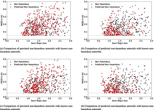
Comparative analysis of non-hazardous asteroid prediction over time with known non-hazardous asteroids: evaluating model performance across time intervals.
From Fig. 9, it can be observed that asteroids that were initially hazardous and predicted as non-hazardous after 0.5 and 1 Myr in the future form a dense cluster in the region between 0.05 and 0.1 au, with the spread gradually decreasing after that, indicating that most MOID values are closer to 0.05 au. Notably, this region was denser for the half-million-year predictions compared to the 1 Myr predictions, suggesting that some of the initially hazardous asteroids were moving away from Earth over time, as indicated by their increasing MOIDs. Fig. 9 provides evidence supporting the decrease in the number of hazardous asteroids over time, particularly among the initially identified hazardous asteroids as shown in Fig. 10(b). However, this clustering pattern is not evident for initially non-hazardous asteroids.
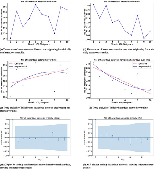
Top panels show hazardous asteroids over time from initially non-hazardous and hazardous groups. Middle panels show trend analysis plots and bottom panels display autocorrelation function (ACF) plots.
After evaluating the predictions made by the decision tree model, we are confident in its reliability and ability to provide meaningful outcomes. Consequently, we divided the numerically integrated data into intervals of 0.1 Myr for both initially non-hazardous and hazardous asteroids and applied the decision tree classifier.
Fig. 10 provides a comprehensive analysis of the temporal evolution and behaviour of hazardous asteroids. Fig. 10(a) illustrates the temporal evolution of hazardous asteroids that were initially classified as non-hazardous, highlighting the number of such transitions over time. Fig. 10(b) depicts the temporal evolution of asteroids that were initially hazardous, showing how their numbers change over time. The number of hazardous asteroids is decreasing over time for those that were initially hazardous. However, no definitive conclusion can be drawn for the initially non-hazardous asteroids based solely on Fig. 10(a).
The trend analysis conducted on the transition dynamics is shown in Figs 10(c) and (d) of initially non-hazardous and hazardous asteroids over 1 Myr reveals significant insights. The transition of initially non-hazardous asteroids into hazardous asteroids displays a positive trend, with the linear regression indicating an increase of approximately 1.442 transitions per 0.1 Myr (slope = 1.442, intercept = 176.467). Despite this observed increase, the low R2 value of 0.165 suggests that the time interval alone explains only 16.5 per cent of the variance in these transitions, indicating the presence of other influential factors. Conversely, the number of hazardous asteroids when starting from initially hazardous asteroids shows a noticeable negative trend, with a decrease of about 3.424 asteroids per 0.1 Myr (slope = –3.424, intercept = 239.133). The R2 value of 0.561 indicates that time is a significant predictor, accounting for 56.1 per cent of the variance in this case. This suggests a more consistent and predictable pattern, highlighting a substantial reduction in the hazardous asteroid population over time. We have also plotted the polynomial regression line (in blue) as shown in Figs 10(c) and (d).
Autocorrelation function (ACF) plot, a fundamental tool in time series analysis, reveals intricate dependencies within sequential observations. In our investigation, these plots illuminated distinct temporal dynamics within two asteroid data sets. Fig. 10(a) shows for initially non-hazardous to hazardous transitions, autocorrelation analysis unveiled a lack of significant temporal correlation, indicating a seemingly random evolution over observed time intervals. Conversely, the analysis of initially hazardous asteroids, as shown in Fig. 10(b), revealed a weak but noticeable temporal dependency, with a positive autocorrelation at lag 1 and 2, signifying a slight predictive relationship between successive time points. However, this effect diminished gradually, with autocorrelation weakening beyond lag 2. These findings suggest that while the transition of initially non-hazardous asteroids to hazardous status lacks discernible temporal patterns, the process for initially hazardous asteroids exhibits a degree of persistence, albeit with diminishing influence over longer time intervals. Such insights offer valuable contributions to models forecasting asteroid behaviour and enhance our understanding of the nuanced stability and transition dynamics characterizing asteroid hazardousness over extended periods.
During the long-term evolution of the asteroids, many from both groups – initially non-hazardous and initially hazardous –were ejected from our Solar system. Fig. 11 illustrates the number of ejected asteroids from each group, respectively, in intervals of 100 000 yr. These figures provide insights into the dynamics of asteroid ejections over extended periods, shedding light on the overall stability and evolution of our Solar system’s NEAs population. No apparent trend or autocorrelation was observed in the ejection rates for both initially non-hazardous and hazardous asteroids over time. The number of ejections appears to be randomly distributed across the time intervals, with no evident dependencies or systematic patterns detected.
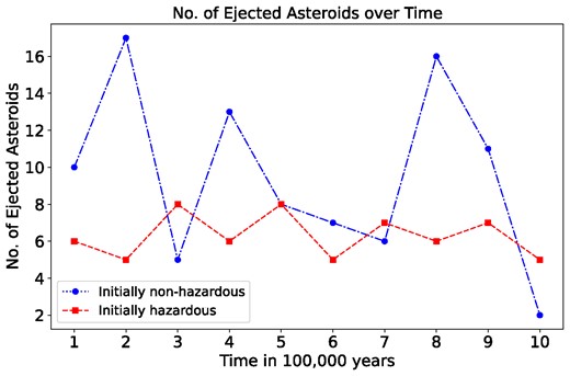
Comparison of the number of ejected asteroids over time between initially non-hazardous (1094) and initially hazardous (569) asteroids.
Upon examining the orbital elements of ejected asteroids over time, we observed two primary ejection patterns. In the first pattern, the asteroids exhibited semimajor axes between 1 and 3 au, coupled with highly eccentric and inclined orbits before their eventual ejection. In the second pattern, the semimajor axes of the asteroids remained stable for extended periods due to resonance (Dvorak 1999), as demonstrated in Fig. 12(d) and then a sudden increase in its semimajor axis possibly due to a close encounter with a planet. The oscillatory nature of the eccentricities, indicative of long-term resonance effects, is evident in Fig. 12(b).
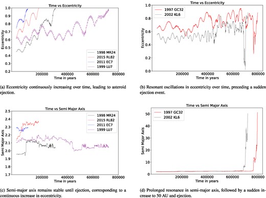
Two ejection patterns of asteroids: gradual eccentricity increase driven by perturbations, and sudden ejection following a close encounter.
The ejection of asteroids from the Solar system, as demonstrated by time versus eccentricity and time versus semimajor axis in Fig. 12, can be attributed to several key dynamical processes. First, resonant interactions play a significant role. Mean motion resonances with major planets like Jupiter and Saturn can trap asteroids, gradually increasing their eccentricity until their orbits become unstable and they are expelled from our Solar system. Secular resonances, involving long-term gravitational influences, can also alter an asteroid’s orbital parameters over extended periods. Second, close encounters with major planets can cause substantial gravitational perturbations, especially when repeated, potentially accelerating asteroids to velocities exceeding the escape velocity.
In Fig. 12(a), we see that the pattern is characterized by a continuous oscillation and increase in eccentricity until the asteroid is ultimately ejected from the Solar system. This behaviour suggests a gradual accumulation of perturbations that steadily drive the asteroid’s orbit towards hyperbolic escape, indicating a long-term dynamical instability possibly influenced by consistent gravitational interactions with planetary bodies or other asteroids.
The observed ejection pattern in Figs 12(b) and (d) underscores the dual influence of resonances and close encounters in asteroid dynamics. A resonance with a major planet initially maintains the asteroid in a stable, oscillatory orbit. However, the resonance can break down due to various cumulative effects, leading to a close encounter with a planet. This encounter dramatically alters the asteroid’s orbital parameters, increasing its semimajor axis and eventually resulting in its ejection from the Solar system. This scenario highlights the complex interplay between long-term stable configurations and sudden dynamic changes driven by gravitational interactions.
7 CONCLUSIONS
In this study, we explored the application of ML techniques to classify and predict the behaviour of asteroids, particularly focusing on NEAs and their potentially hazardous nature. Our work commenced with an overview of asteroids, historical impacts, and the critical importance of early detection for deflection strategies. Given the vast number of asteroids and the extensive data on their properties and orbits, manual analysis is impractical, making ML an ideal tool for this task.
We employed seven different ML models – ANN (MLP), KNN, decision tree, RF, ExtraTree, AdaBoost, and Gboost – on a comprehensive data set of 4687 asteroids. These models were used to classify asteroids into NEAs (specifically Atens, Amors, Apollos, and Apoheles) and non-NEAs, further categorizing them into potentially hazardous and non-hazardous groups. Following this, we applied the Mercury N-body integrator to simulate the orbits of over 1650 initially hazardous and non-hazardous asteroids.
We employed the Mercury N-body integrator for the integration process, utilizing symplectic techniques to simulate gravitational interactions among multiple celestial bodies within complex planetary systems. The integration was conducted under two scenarios: one incorporating non-gravitational perturbations, such as the Yarkovsky effect, solar radiation pressure, and thermal forces, and another excluding these perturbations. Due to the significantly smaller magnitude of these non-gravitational perturbations relative to the gravitational perturbations, no discernible differences in the results were observed over the 1 Myr numerical integration period.
We also carefully addressed model validation and the overfitting problem. Specifically, we employed k-fold cross-validation to better assess the models’ generalization capability. A large unseen data set of more than 35 000 asteroids was used to validate the models and assess their predictive power. For all seven models, strategies to mitigate overfitting were implemented, such as regularization and early stopping. Regularization was applied across all models to limit complexity. For models like decision tree, random forest, extra tree, and boosting algorithms, regularization involved restricting model complexity through hyperparameter tuning to prevent overfitting. Additionally, evaluation metrics such as accuracy, precision, recall, F1 score, macro average, weighted average of F1 scores, MCC, and the AUC-PR curve were used to evaluate the models’ predictive power.
Among the models, decision tree, AdaBoost, and Gboost consistently performed the best across both classification tasks, as evidenced by the evaluation metrics and their performance on the large unseen data set. Random forest also performed well but exhibited slightly higher false prediction rates compared to the top three models. Conversely, KNN was the worst-performing model overall, while MLP and ExtraTree showed acceptable but not exceptional performance.
We applied the best-performing model for predicting NEAs and non-NEAs over time. The temporal analysis reveals that initially hazardous asteroids exhibit greater dynamic changes, particularly in their transition rates and population stability, compared to initially non-hazardous asteroids. Overall, the stability of different asteroid groups varies, with certain groups demonstrating more resilience and others showing significant fluctuations over time. These findings underscore the diverse evolutionary dynamics and stability patterns among the asteroid populations over extended periods.
Further for the second classification, our model’s performance was excellent while predicting the unseen data that we obtained after half a million years and 1 Myr of numerical integration. It predicted all the data accurately into hazardous and non-hazardous asteroids. This validation allowed us to confidently scale up our predictions. We divided the 1 Myr integration into 10 intervals of 100 000 yr each, predicting hazardous and non-hazardous asteroids over time. Our analysis revealed a pattern where initially hazardous asteroids tended to become non-hazardous, while initially non-hazardous asteroids showed no clear time-based trend, fluctuating randomly between hazardous, and non-hazardous states. Additionally, two ejection patterns were found when eccentricity and semimajor axis of asteroids were compared with time (Fig. 12).
Overall, our study highlights the effectiveness of ML models in asteroid classification and prediction, providing a robust framework for large-scale application and offering valuable insights into asteroid behaviour over extended periods.
ACKNOWLEDGEMENTS
We extend our gratitude to the Inter-University Centre for Astronomy and Astrophysics (IUCAA) in Pune for granting access to their off-campus research resources through the Visiting Associateship program.
DATA AVAILABILITY
We acknowledge the use of the data from the Kaggle (https://www.kaggle.com/datasets/shrutimehta/nasa-asteroids-classification) compiled by Shruti Mehta and all the data are from the http://neo.jpl.nasa.gov/. The API is maintained by SpaceRocks Team: David Greenfield, Arezu Sarvestani, Jason English, and Peter Baunach. We also acknowledge the use of data from NASA JPL Solar System Dynamics. (Downloaded 2024, July, 08). (Small-Body Database Query). https://ssd.jpl.nasa.gov and Minor Planet Center (MPC) (https://www.minorplanetcenter.net/iau/mpc.html). The Minor Planet Center functions within the Smithsonian Astrophysical Observatory (SAO), under the guidance of Division F of the International Astronomical Union (IAU), and receives its funding through a NASA grant.
