


ABSTRACT
The characteristics of the young stellar population in the nearby irregular galaxy NGC 2366 were investigated. In particular, we focused our attention on its hierarchical clustering distributions and the properties of the stellar groups. This galaxy exhibits a prominent blue helium-burning star feature in the colour-magnitude diagram, suggesting that it has undergone an extended period of stellar formation. The galaxy was observed in two bands by the Hubble Space Telescope covering almost its complete central and intermediate parts, including all the major stellar formation regions. Available photometric data allowed us to select the blue and young stars and, therefore, study the recent stellar formation. Through the path linkage criterion (PLC), we found 23 young star groups and estimated their fundamental parameters, such as their stellar densities, sizes, and number of members. We also performed a fractal substructure analysis to determine the clustering properties of this population, and we built a stellar density map corresponding to the galactic young population. We found that most of the young stellar groups have stars that have a distribution of locations that is compatible with a fractal dimension.
1 INTRODUCTION
NGC 2366 (DDO 42) is a nearby irregular galaxy with an angular size of 8.1 × 3.3 arcmin. The older stars of this galaxy show an elliptical centrally concentrated structure, whereas the younger blue stars are scattered through the main body with few highly concentrated regions (Weisz et al. 2008). As might be expected in a galaxy with an active stellar formation, several H ii regions are present in it, with a prominent star formation region on the southern edge (Sandage & Bedke 1988). Weisz et al. (2008), analysing the SFR by the observed stellar population, show that NGC 2366 has been very actively forming stars in the last 1 Gyr. Also, NGC 2366 is known as a cometary galaxy with a head and a tail, and a high surface brightness star-forming region is observed on both, the head and the end of the tail.
Photometry of the brightest stars in the galaxy yielded distance moduli of 27.14 (de Vaucouleurs 1978) and 27.69 mags (Tikhonov et al. 1991). Additionally, de Vaucouleurs (1978) considered that NGC 2366 forms a pair with NGC 2403 galaxy since they seem to share the same distance and redshift. Karachentsev et al. (2002) found that the position of the tip of the red-giant branch (TRGB) at 23.54 ± 0.28 mag, giving the true distance modulus of 27.52 mag. As it is noted by Petit, Drissen & Crowther (2006), this value is in very good agreement with the value of |$(m-M)_0= 27.68 $| mag determined from a long-term study of the Cepheids in NGC 2366 by Tolstoy et al. (1995). As it was done by Petit et al. (2006), we took an average value of the distance module as |$(m-M)_0=27.6 $| mag that it would correspond to a distance of 3.3 Mpc. This last value was adopted for this work and implies a scale of 16 pcs arcsec−1 over the sky.
In this paper, we took advantage of the exceptional data quality acquired through the Hubble Space Telescope (HST), which provides a resolution capable of isolating individual stars, thus ensuring high-quality data without almost any crowding contamination. This allowed us to study the young stellar groups (YSGs) within NGC 2366 and extract their fundamental characteristics. So in this work, we consider that YSGs have sizes from open clusters to large associations of young OB blue stars.
We focused our work on the exploration of these formations since it has been observed in several galaxies experiencing substantial stellar formation that the arrangement of stars within these groups seems to display a fractal pattern, conceivably inherited from the turbulence of the initial gas cloud where the stars originated. The properties of the gas turbulence have been an important factor in the characterization of the interstellar medium, which has been shown to exhibit fractal behaviour; see, for example, the study of Elmegreen (1997). Therefore, the primary focus of this paper is to examine the YSGs structure to determine whether a fractal pattern is indeed present.
This work is organized as follows: In Section 2, we describe the observations and photometry data used in this research. Section 3 describes the colour-magnitude diagram properties of the observed population. In Section 4, we discuss the methods used to identify the young stellar population and the search for stellar groups inside this population. Section 5 presents a morphological analysis of the detected groups and structures. Finally, in Section 6, we take out our conclusions.
2 OBSERVATIONS AND DATA
In the present paper, we used photometric information from images obtained with the Wide Field Camera (WFC) from the Advanced Camera for Surveys (ACS) on board the HST. The WFC has a mosaic of two Charge-Couple Devices (CCD) detectors with a field of view of 3.3 × 3.3 arcmin and a scale of 0.049 arcsec pixel−1, which is a projected scale of 0.8 pc pixel−1 at the adopted galaxy distance.
We selected the images provided by the Hubble Legacy Archive1 corresponding to two fields that cover a significant area of NGC 2366. The observations were carried out in September 2006 during the HST Cycle 15 as part of the program GO-10605 (PI: Skillman, Evan D.); see Table 1. These data encompassed the central part of the galaxy, the bar, and the most prominent regions of star formation (see Fig. 1). Each field was observed using the broad-band HST/WFC filters F555W and F814W.
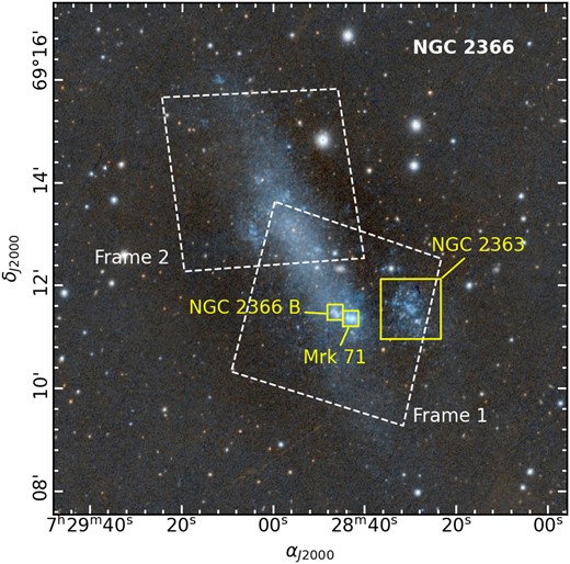
PanSTARRS DR1 colour image from Aladin. It is centred in NGC 2366 galaxy and covers a 10 × 10 arcmin field of view. Big white slashed shapes indicate the HST/ACS footprints studied in this work.
Observations details.
| Field | Filter | Nexp | |$t_{\rm exp}$| [sec.] | Date |
|---|---|---|---|---|
| 1 | F555W | 2 | 4780 | 2006-11-10 |
| 1 | F814W | 2 | 4780 | 2006-11-10 |
| 2 | F555W | 2 | 4780 | 2006-11-12 |
| 2 | F814W | 2 | 4780 | 2006-11-12 |
| Field | Filter | Nexp | |$t_{\rm exp}$| [sec.] | Date |
|---|---|---|---|---|
| 1 | F555W | 2 | 4780 | 2006-11-10 |
| 1 | F814W | 2 | 4780 | 2006-11-10 |
| 2 | F555W | 2 | 4780 | 2006-11-12 |
| 2 | F814W | 2 | 4780 | 2006-11-12 |
2.1 Photometry
The photometric data used in this work were obtained from the MAST data base of the Space Telescope Institute (STScI).2 They correspond to the ‘star files’ of the ACS Nearby Galaxy Survey (ANGST). These photometric tables provided ‘point spread function’ photometry. It was carried out by Dalcanton, Williams & ANGST Collaboration (2008), using the software DOLPHOT3 adapted for the ACS (Dolphin 2000).
The produced tables contain the photometry of all objects classified as stars with good signal-to-noise values (S/N > 4) and error flag <8 (See ANGST description of this flag).
Fig. 2 shows the photometric errors in each band corresponding to the objects classified as stars in the two fields. This figure shows that the sample remains reliable up to magnitude 26 in both bands. Therefore, we choose F555W = 24 as the threshold value to define a sample with minimal errors. This choice ensures that, for instance, a colour-magnitude diagram (CMD) used for star classification would maintain a high level of accuracy. We also built the F555W luminosity function (LF) for the two fields (see Fig. 3) to evaluate the completeness of the data. Fig. 3 shows that the number of stars per bin starts to decrease at F555W ∼ 27.5. Therefore, we considered that the sample is complete up to this value, so the threshold value of F555W = 24 also appears to be a suitable choice for assessing data completeness. A blue star with this magnitude at the galaxy is type B0 on the main sequence.

Photometric errors in the different bands. Errors increase significantly at magnitude 26. Therefore, we will limit the utilization of data to magnitude 24 (represented by the green line) to mitigate substantial errors.
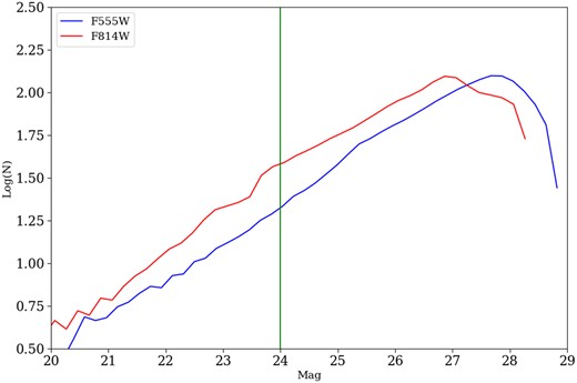
The luminosity function for the two examined fields based on the F555W data. The sample exhibits a high degree of completeness, extending up to a magnitude of 27. The green line, set at F555W = 24 mag, represents the magnitude limit employed in this study.
2.2 Astrometric correlation of tables
The ANGST tables provide astrometric and two bands of photometric information in two fields of NGC 2366 (see Fig. 1). Since these fields are slightly overlapping, we could measure small astrometric differences between them (see first line in Table 2). Differences in the magnitude of common objects were 0.01 mag. We produced then a uniform single table with approximately 6.3 × 10⁵ objects using STILTS.4 We also compared the astrometric information provided by ANGST tables with that given by Gaia DR3 catalogue (Gaia Collaboration et al. 2016, 2023) for those objects in common. We obtained the differences presented in Table 2, and they were used to correct the given ACS/HST coordinates.
Astrometric differences of ACS/HST data.
| Fields | |$\Delta \alpha$| | |$\Delta \delta$| |
|---|---|---|
| Frame 1 − Frame 2 | −3.60 arcsec | 0.69 arcsec |
| Frame 1 − Gaia | −0.31 arcsec | 0.41 arcsec |
| Frame 2 − Gaia | −3.91 arcsec | 1.10 arcsec |
| Fields | |$\Delta \alpha$| | |$\Delta \delta$| |
|---|---|---|
| Frame 1 − Frame 2 | −3.60 arcsec | 0.69 arcsec |
| Frame 1 − Gaia | −0.31 arcsec | 0.41 arcsec |
| Frame 2 − Gaia | −3.91 arcsec | 1.10 arcsec |
2.3 Star blend and foreground contamination
Star blends can be found in cases in which two (or more) unrelated stars are close enough to be considered as one object. DOLPHOT provides for each detected object, its astrometry, photometry, and the parameters of the PSF fit. These latter values are sharpness, crowding, S/N, and |$\chi ^2$|, and they are a good estimator of the quality of the measurement and a reference for detecting blended stars. The most problematic case is when two stars are located at the same position of a pixel and therefore mistakenly detected as only one object. These particular situations cannot be identified using the above-indicated fitting parameters. However, it is possible to model this effect.
An estimation of the maximum level of blending can be calculated by measuring the maximum star density in the galaxy and assuming that this stellar density is constant over the whole object. Thus, the blending effect can be modelled considering that the stars are distributed with a Poisson distribution. This is equivalent to the procedure of Kiss & Bedding (2005), which is discussed deeply for these kinds of observations in Feinstein et al. (2019). Therefore, this model allows us to obtain an upper limit of the probability of blends for crowded regions that are larger than the probability of less populated places. By this procedure, we obtained that the probability of losing stars by blends is <3 per cent in more crowded locations of the galaxy, corresponding to lower values in the other regions. Therefore, we concluded that this is not an important issue in this work.
Another way to lose stars is in the bright H ii regions where the Hα emission and other lines are very bright, so make a high-intensity background. So, the local stars are difficult to measure because faint stars are confused with the high-level background (note the F555W filter includes the Hα emission and other emission lines). But, there is a very easy way to account for this incompleteness. This is plotting the stars of the galaxy for several ranges of magnitude. By doing this, we found that there are holes in the stellar distributions over the H ii regions, beginning at 26.5 F555W magnitude. So, our sample is at least unaffected for brighter magnitudes than 26.5.
One possible source of data contamination could be the galactic stars in the field of view of NGC 2366. The galactic coordinates of our target are |$l = 146.41^{\circ }$|, |$b = 28.53^{\circ }$|, which locates it at somewhat medium to low latitude on the Milky Way. This means that the probability of contamination of our sample by blue galactic stars must be accounted for. In order to check this possible contamination, we ran several simulations with the Trilegal web site5 (Girardi et al. 2012). We used these models of our galaxy to find the number of Milky Way stars projected on the region of the observations. We found that the total galactic stars are on average about 100, but most of them show to be faint, have very red colours, or show both features. As our interest is in the region of the brighter blue stars on the CMD, the number of galactic stars from the models shown to be on average lower than 20. So, we considered the contamination as negligible because in the bright blue region of CMD, our sample has more than 12 000 stars. Therefore, we do not consider the galactic contamination as a problem for the analysis of young blue clusters because the number of stars is too low in comparison with the observed stars in the field (∼0.16 per cent). Also, the obvious bright galactic stars that saturated the CCD counts were eliminated from our final work data.
3 COLOUR MAGNITUDE PROPERTIES
The photometric information allowed us to build the corresponding photometric diagrams. Fig. 4 presents a combination of the Hess diagram with the conventional CMD. It provides insights into the high density of stars in various regions of the plot and individual stars in regions corresponding to lowest density values. The obtained diagram displays a diverse array of stars in various stages of evolution. Among them, the main-sequence (MS) stars are prominently visible, characterized by their hydrogen-burning cores. Adjacent to the MS, we find the blue helium-burning stars (BHeBs), which are intermediate-mass stars (likely between 2–15 M|$_{\odot}$|) that have progressed beyond the MS phase and are currently undergoing helium burning in their cores. Moving further to the right, we observe the red helium-burning stars (RHeBs). To the right of the plot, albeit fainter, we encounter the asymptotic giant branch stars (AGBs), which are low- to intermediate-mass stars that have evolved to the point of burning both hydrogen and helium in shells surrounding their cores. It is also possible to distinguish the red giant branch (RGB) and its tip. At fainter magnitudes, the RGB branch, RHeBs, and the red clump overlap, resulting in a region with higher stellar density in the diagram.
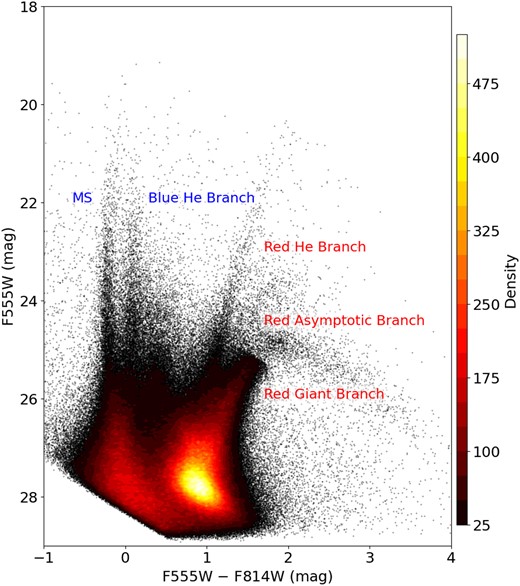
A combination of a Hess diagram and CMD (F555W versus F555W − F814W) depicting the detected objects in the two studied fields of NGC 2366. The use of different colours in the diagram indicates varying densities, ranging from black (lower densities) to yellow (higher densities). The plot showcases distinct populations, with a particular focus on very young stars that appear to be part of an ongoing and continuous burst of stellar formation dating back approximately 50 Myr. Prominent helium sequences are present on both the right and left sides, indicating the presence of stars in different evolutionary stages. Additionally, the diagram displays the red asymptotic branch, the red giant branch, and its tip.
Our focus lies on recent stellar formation, primarily represented in the CMD by the MS stars that are clearly seen in Fig. 4. Consequently, we distinguish the blue population, consisting of MS star from the other branches and regions, which we categorize as the red population. To identify member stars belonging to each population, we employ the following criteria:
Bright stars: |$F555W \le 24$|
Blue population: |$F555W-F814W < {-}0.06$|
Red population: |$F555W-F814W > 0.6$|.
By applying this criterion, we generated Fig. 5. The orange box on the plot encompasses the MS objects, essentially representing the young blue stars that we will analyse in this paper. The red data points, indicating older stars, have already been examined in Weisz et al. (2008). Also, in this figure, we overlapped the PARSEC version 1.2S evolutionary model (Tang et al. 2014) corresponding to some particular ages (107, 108, and 109 yr) and metallicity |$z = 0.0027$| (Marigo & Girardi 2007) to have a comparison with the different galaxy stellar populations. These isochrones were displaced adopting a distance modulus of |$(V_0-M_V)$| = 27.6 Petit et al. (2006), a normal reddening law (|$R = A_V /E(B-V)$| = 3.1), and a value for |$E(B-V)$| = 0.0387, corresponding to the foreground reddening toward NGC 2366, (Schlafly & Finkbeiner 2011). The following coefficients were used to transform these values to the HST system: |$A_{F555W}/A_V$| = 1.035 and |$A_{F814W}/A_V$| = 0.6056 (O’Donnell 1994). This model fits the MS and shows that the average parameters (extinction, metallicity, distance, and age) agreed with the data.
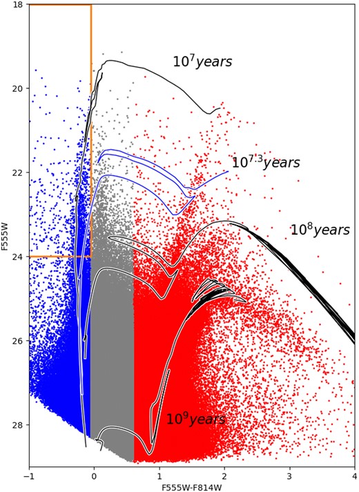
CMD (|$F555W$| versus |$F555W-F814W$|) detailing different stellar populations. The younger and older populations with blue and red symbols, respectively. The orange rectangle encloses the bright blue stars that were used for selecting and searching the YSGs. Grey curves indicate PARSEC version 1.2S isochrones (Tang et al. 2014) corresponding to different ages and metallicity |$z = 0.0027$|. This model was displaced, adopting a distance modulus of |$(V_0-M_V)$| = 27.6 (Petit et al. 2006), a normal reddening law (|$R = A_V /E(B-V)$| = 3.1), and a value for |$E(B-V)$| = 0.033, corresponding to the foreground reddening toward NGC 2366 (Schlafly & Finkbeiner 2011).
Moreover, both Figs 4 and 5 show a significant feature: the presence of abundant stars in both the BHeBs and the RHeBs. Typically, the RHeBs are commonly found in galaxies of this kind, while the BHeBs are less prevalent and often appear faint and less distinct. Stars spend a shorter time in the BHeBs compared to the MS phase, and this duration mainly depends on the star’s mass. In a scenario where stars form over an extended period of time, they would undergo evolutionary processes, transitioning from the main sequence (MS) to the BHeBs. Concurrently, new stars would replace the ones that move from the MS to the BHeBs branch, resulting in a continuous population of stars in the BHeBs branch. However, if stellar formation were to cease, the stars in the BHeBs branch would evolve without being replaced by new stars from the MS. As a consequence, this branch would vanish quicker than the MS, starting with the more massive stars first. In such a situation, the absence of new stars to replenish the BHeBs branch would lead to its eventual disappearance. In the context of this galaxy, the presence of the BHeBs suggests a continuous stellar formation rate (SFR) that has persisted for at least |$10^9$| yr. Weisz et al. (2008) has a detailed discussion of the photometric characteristics of the stellar populations in this galaxy and an analysis of the more probable history of the SFR in the object.
4 THE SEARCH FOR YOUNG STELLAR GROUPS
4.1 Identification of the various star populations
For detecting and characterizing the YSGs, we are going to use only the bright blue stars of Fig. 5. This sample consists of stars in the region inside the |$F555W \le 24$| and |$(F555W-F814W) < -0.06$| box. These criteria allow us to ensure a low degree of contamination from low-quality observations and, on the other hand, a sample of bright blue young stars. This sample is going to include clusters and foreground objects. Iorio et al. (2017) determined that the galaxy has an inclination of |$i=65^{\circ }$| with a position angle of PA = 35°. These parameters allowed us to deproject sky coordinates to estimate the real spatial position of the stars for the selected sample. The obtained deprojected coordinates were used to look for YSGs, minimizing false identifications of some clusters produced by an inclined perspective.
4.2 The searching algorithm
We used the path linkage criterion (PLC) from Battinelli (1991) over the bright blue population to detect YSGs in the galaxy. Details of the applied procedure were presented in our previous works (Rodríguez, Baume & Feinstein 2016, 2018, 2020). Briefly, the PLC is an agglomerative friend-of-friend algorithm that links stars using a searching distance scale |$d_{\rm s}$| and considering a minimum number of stars (ρ) to define a stellar group. Therefore, in this method, the stars of a particular YSG are each one at a distance less or equal a prederminate separation between them. So, if an star is at a distance less or equal than a critical distance (|$d_{\rm s}$|) from an already considered member to the YSG. So, this object is also considered a member and then is use for testing for others starts in the neighbourhood that have also a separation less or equal than |$d_{\rm s}$|. This process repeat until no more new stars are found. If the group of stars found have less than ρ members these stars are not considered as forming an YSG. Then another star is considered as a reference object and then the process is repeated until all stars in the sample are tested and all the possible YSGs are detected.
In Battinelli’s paper (Battinelli 1991), an algorithm is presented for determining the appropriate critical distance (|$d_{\rm s}$|) in a sample of stars. This process involves testing various quantities of members and different values of |$d_{\rm s}$|. The author demonstrates that, for a fixed number of stars to be considered as a group, starting with the minimal distance between two stars in the sample as the value of |${d_{\rm s}}$| and then incrementing it, the number of YSGs would increase until the groups begin to merge, at which point the number would begin to decrease. Therefore, the optimal value of |${d_{\rm s}}$| for the sample would be the one that maximizes the number of groups obtained. In other worlds, the proper |$d_{\rm s}$| is found as a maximum in the plot of the number of groups found for a fixed number of members in some of range of |$d_{\rm s}$|.
Fig. 6 shows the number of YSGs detected as a function of |$d_{\rm s}$| for different quantity of numbers of members in the group.
We can see that the maximum of the distribution falls around |$0{_{.}^{\prime\prime}} 38$| (∼6 pc over the galaxy). Following Battinelli (1991), this maximum is considered to indicate the optimal value of |$d_{\rm s}$|. For the search of the YSGs over the galaxy data, we used |$p=8$| value we considered optimum from previous work; this means that any YSG found must have at least 8 members. For example, Pietrzyński et al. (2001) use |$p=6$| members for the search of OB associations on the spiral galaxy NGC 300.
As indicated in Battinelli’s paper, PLC method can be likened to the minimal spanning tree (MST) algorithm. However, the MST method itself is not a cluster classification technique; rather, it constructs a graph containing all the objects in a given dataset as vertices. The total edge length connecting two vertices is minimized in this graph. It’s evident that both the MST and the PLC yield the same classification when an upper cut-off for the edge lengths is adopted as the edge-breaking criterion. In other words, when all edges longer than a certain scale |$d_{\rm s}$| are removed.
PLC method was implemented as a python function therefore it was easy to integrate its outputs with Scikit-Learn7 package. This module provides several packages to test the quality of the identified clusters therefore we evaluate the obtained results using three of these tests that are sensitive to density: the Silhouette Coefficient, the Calinski-Harabasz Index, and the Davies–Bouldin Index. In all these cases, we computed a positive response at |$d_{\rm s} = 0{_{.}^{\prime\prime}} 38$| as the best search radius. Refer to Table 3 for the identified YSGs and their key properties.
Regions data.
| Id | |$\alpha _{2000}$||$\delta _{2000}$| | |$F555W_{\min}$| | #Stars | |$D_{\rm cg}[{\rm Kpc}]$| | Radius[pc] | |$\rho$|[obj./pc|$^{-2}$|] | |$\overline{m}$| | |$\overline{s}$| | Q |
|---|---|---|---|---|---|---|---|---|---|
| (1) | (2) | (3) | (4) | (5) | (6) | (7) | (8) | (9) | (10) |
| 1 | 07:28:42.8 69:11:22.2 | 19.54 | 9.0 | 1.14 | 7.4 | 0.0523 | – | – | – |
| 2 | 07:28:43.7 69:11:23.7 | 19.83 | 32.0 | 0.95 | 23.36 | 0.01866 | 0.54 |$\pm$| 0.04 | 0.79 |$\pm$| 0.05 | 0.68 |$\pm$| 0.05 |
| 3 | 07:28:43.3 69:11:21.4 | 19.9 | 15.0 | 1.02 | 11.1 | 0.03878 | – | – | – |
| 4 | 07:28:42.9 69:11:21.3 | 20.0 | 81.0 | 1.09 | 38.78 | 0.01714 | 0.54 |$\pm$| 0.03 | 0.75 |$\pm$| 0.04 | 0.72 |$\pm$| 0.04 |
| 5 | 07:28:42.5 69:11:22.4 | 20.45 | 10.0 | 1.2 | 10.37 | 0.02958 | – | – | – |
| 6 | 07:28:42.4 69:11:20.2 | 20.46 | 19.0 | 1.19 | 20.16 | 0.01488 | – | – | – |
| 7 | 07:28:42.7 69:11:22.8 | 20.52 | 12.0 | 1.16 | 9.49 | 0.04241 | – | – | – |
| 8 | 07:28:42.5 69:11:21.5 | 20.68 | 9.0 | 1.19 | 9.48 | 0.03189 | – | – | – |
| 9 | 07:28:43.9 69:11:22.4 | 21.16 | 42.0 | 0.9 | 30.88 | 0.01402 | 0.49 |$\pm$| 0.04 | 0.79 |$\pm$| 0.05 | 0.61 |$\pm$| 0.05 |
| 10 | 07:28:43.0 69:11:23.4 | 21.16 | 9.0 | 1.1 | 10.83 | 0.02442 | – | – | – |
| 11 | 07:28:42.4 69:11:22.9 | 21.39 | 36.0 | 1.24 | 22.42 | 0.02279 | 0.63 |$\pm$| 0.05 | 0.86 |$\pm$| 0.06 | 0.73 |$\pm$| 0.05 |
| 12 | 07:28:45.9 69:11:25.4 | 21.64 | 8.0 | 0.5 | 10.83 | 0.0217 | – | – | – |
| 13 | 07:28:43.3 69:11:20.2 | 21.73 | 14.0 | 1.0 | 13.9 | 0.02308 | – | – | |
| 14 | 07:28:45.9 69:11:24.1 | 21.78 | 27.0 | 0.49 | 21.1 | 0.0193 | 0.5 |$\pm$| 0.05 | 0.77 |$\pm$| 0.06 | 0.65 |$\pm$| 0.05 |
| 15 | 07:28:43.4 69:11:22.1 | 21.92 | 11.0 | 0.99 | 10.44 | 0.0321 | – | – | – |
| 16 | 07:28:46.2 69:11:25.8 | 21.97 | 8.0 | 0.44 | 6.52 | 0.05987 | – | – | – |
| 17 | 07:29:04.0 69:13:01.6 | 22.06 | 8.0 | 1.96 | 10.47 | 0.02323 | – | – | – |
| 18 | 07:28:43.9 69:11:20.9 | 22.18 | 35.0 | 0.87 | 24.01 | 0.01933 | 0.52 |$\pm$| 0.04 | 0.82 |$\pm$| 0.04 | 0.64 |$\pm$| 0.05 |
| 19 | 07:28:43.8 69:11:21.2 | 22.51 | 8.0 | 0.89 | 7.67 | 0.04334 | – | – | – |
| 20 | 07:28:43.7 69:11:24.9 | 22.58 | 20.0 | 0.97 | 14.05 | 0.03223 | 0.71 |$\pm$| 0.06 | 0.91 |$\pm$| 0.08 | 0.78 |$\pm$| 0.05 |
| 21 | 07:28:43.2 69:11:21.8 | 22.81 | 8.0 | 1.04 | 11.48 | 0.01932 | – | – | – |
| 22 | 07:28:42.2 69:11:20.6 | 22.86 | 15.0 | 1.25 | 14.66 | 0.02222 | – | – | – |
| 23 | 07:28:43.7 69:11:19.0 | 23.25 | 9.0 | 0.89 | 8.52 | 0.03943 | – | – |
Notes: Columns: (1): Identification; (2): RA & DEC J2000 coordinates; (3): F555W value of the brightest blue star; (4): total number of bright blue stars; (5): Galactocentric distance; (6): radius of the group; (7): surface density of star in the YSGs; (8): mean edge length in an MST (|$\overline{m}$|) and its error (|$e_{\overline{m}}$|); (9): mean separation of the stars in the group (|$\overline{s}$|) and its error (|$e_{\overline{m}}$|); (10): Q parameter and its error (|$e_{Q}$|).
4.3 Stochastic clusters
To determine the likelihood of encountering stochastic clusters purely by chance, we performed simulations on stellar fields characterized by a consistent density of |$\rho = 0.105$| stars per square arcsecond (in deprojected coordinates). This density was obtained from measurements in the central regions of NGC 2366, which is higher than the typical density in the most populated regions and even higher than that in the galaxy’s disc regions. Since the other regions are expected to be less populated, the probability of detecting stochastic clusters in those areas is going to be lower.
To these simulations, we applied the PLC method using the same parameters as those used on the real data. We found very few to no clusters in the simulated data. However, when we reduced the distance threshold (|$d_{\rm s}$|) to values lower than |$d_{\rm s} = 0{_{.}^{\prime\prime}} 3$| (the average distance between stars necessary to reproduce the observed density value, |$d_{\rm s} \sim 1/\rho ^{-2}$|), we began to observe a few stochastic clusters. Also by further testing, we found that the minimum of 8 stars to declare a cluster is a hard criterion and eliminates the possibility of chance clusters occurring.
5 FRACTAL SUBSTRUCTURE ANALYSIS
As we have done in our previous works: NGC 247, NGC 300, NGC 253, and NGC 2404 (Rodríguez, Baume & Feinstein 2019, 2020), we investigate the fractal properties of the clustering in the young structures detected using different methodologies. They are presented in the following subsections.
5.1 Measuring the Q parameter
We computed the Q parameter introduced by Cartwright & Whitworth (2004) to distinguish between a smooth large-scale radial density gradient and multiscale fractal clustering. The Q parameter is defined as the ratio of two distinct parameters obtained from the minimum spanning tree (MST) of each cluster, which is the shortest possible network that connects all the stars in the cluster and there are no closed loops. Therefore, the Q parameter is given by:
where: |$\overline{m}$| is the mean edge length in a minimum spanning tree (MST), normalized by the cluster area, |$\overline{s}$| is the mean separation of the points, normalized by the cluster ratio. According to Hetem & Gregorio-Hetem (2019) |$\overline{m}$| parameters can be computed as:
where N is the total number of points (stars in our case), |$m_i$| is the length of edge i in the MST, and |$A_N$| is the area of the smallest circle or convex hull that contains all the points projected on the sky plane. The value of |$\overline{s}$| is calculated as:
where |$r_i$| is the vector position of the star i and |$R_n$| is the radius of the smallest circle or convex hull that contains all the stars. Note that the parameter Q does not depend on the area of the region while |$\overline{m}$| and |$\overline{s}$| parameters do.
Cartwright & Whitworth (2004) found studying artificial clusters that mimic fractal and non-fractal models that values of Q greater than 0.8 correspond to a centrally concentrated distribution for artificial clusters. Conversely, smaller values of Q are indicative of the presence of fractal substructures within the clusters.
We constructed the MST of each YSGs and computed their corresponding Q values for clusters that have more then 20 members, although the limit of 8 members is a good criterium to determined an YSG, this number do no allow to compute a reliable Q parameter. It has been demonstrated that non-fractal clusters with fewer than 20 members can exhibit a Q value within the fractal range (Hetem & Gregorio-Hetem (2019). This discrepancy arises from an inaccurate estimation of the Q parameter due to the loss of the fainter members of the cluster. Hetem & Gregorio-Hetem (2019) shows that for a pair of non-fractal real cluster, when the faint stars are removed from the sample, the Q parameter of this cluster begins to decrease to values lower than |$Q = 0.8$|. So going into the fractal region. Consequently, a sample with a restricted number of members involved in the calculation can result in a significant miscalculation of the Q parameter. Therefore, we selected those clusters with more than 20 bright stars. The result is presented in Fig. 7b.
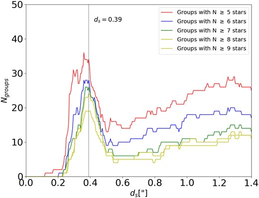
Plot of the number of clusters that have more stars than a certain number (p) for a determined search radius |$d_{\rm s}$|. The calculated curves show a maximum of around |$d_{\rm s} = 0{_{.}^{\prime\prime}} 38$|. It is shown in Battinelli (1991) that the maximum of this curve determined the best |$d_{\rm s}$|.
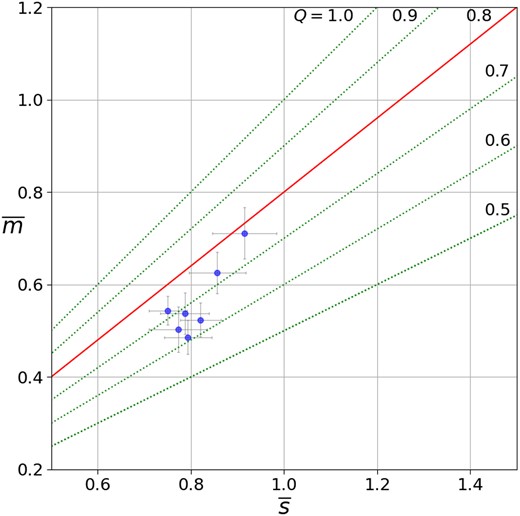
|$\overline{m}$| versus |$\overline{s}$| for the identified YSGs. Lines are for different Q values. The plot includes the YSGs that have more than 20 stars. The data reveals that the Q values for this YSGs are very probably having a fractal dimension. Errors are from bootstrapping calculations.
We found that almost every identified YSGs in NGC 2366 with more than 20 members has Q values corresponding to a fractal behaviour (Q < 0.8). See Fig. 7.
5.2 Morphological structure analysis
In the study by Mandelbrot (1982), the concept of the fractal dimension (D) was introduced as a parameter to quantify the level of irregularity exhibited by an object. When dealing with an object distributed uniformly in space, its fractal dimension assumes a value of 3 (|$D_3 = 3$|), while in a two-dimensional space, |$D_2$| takes on the value of 2. If the object has irregularities D3 < 3 or D2 < 2, respectively. Therefore, these parameters will take smaller values as the object becomes more irregular. The estimation of the two-dimensional fractal dimension (D2) can be achieved through the utilization of the perimeter-area relationship: |$P \propto A^{D_P/2}$|, as outlined by Mandelbrot (1982) applied over a density map. The parameter |$D_P$| characterizes the manner in which an object’s contour occupies space. When considering smoother shapes akin to a circle, |$D_P$| equates to 1 (|$P \propto A^{1/2}$|), while intricate object contours tend towards an occupation of all available space, resulting in |$D_P$| assuming the value of 2 (|$P \propto A$|), as noted by (Sánchez & Alfaro 2010).
For applying this analysis to NGC 2366, we constructed a surface stellar density map for all the young blue stars up to |$F555W=24$| mag over the deprojected galaxy. This magnitude at the galaxy distance correspond to a |$B_0$| stars with a main sequence lifetime of 10 myr or less. The density map was obtained using the kernel density estimation (KDE) method. That is, we replaced each star with a Gaussian kernel. For selecting the corresponding bandwidth of the kernel, we use the analysis given by Rodríguez et al. (2019). Therefore, we built different stellar density maps using this bandwidth value and lower ones, checking in all cases that the main structures were still preserved and that these structures complement those ones found using the PLC method. We finally adopted a bandwidth of |$2{_{.}^{\prime\prime}} 0$|. The final stellar density map of the bright blue stars is presented in Fig. 9. In this procedure, we used the KernelDensity routine from the Python scikit-learn8 library.
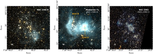
Detailed views of the Markarian 71 H ii region, NGC2366 B, and the core of NGC 2363 galaxy from ACS/HST data. The main features of Mrk 71 (Gonzalez-Delgado et al. 1994) are also indicated.
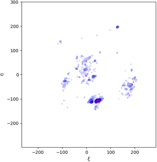
Stellar density map for the blue young stars up to |$F555W = 24$| mag in the deprojected galaxy. The top is North and the left is East. |$\xi$| and |$\eta$| coordinates are in arcsecond from the centre of the galaxy. Red points indicate the location of detected clusters and their size is proportional to the size of YSGs.
The large stellar formation regions MK71, NGC 2366 B, and NGC 2363 presented in Fig. 8 are distinctly discernible in the stellar density map of Fig. 9. Furthermore, they are partitioned into multiple YSGs by the PLC algorithm, as they are not composed of a single concentration of stars but of many YSGs.
Our analysis of the data reveals that the young stellar component follows a relationship where |$P \propto A^{D_P/2}$| with |$D_P =1.02\pm 0.01$|, within the range of sizes where regions are resolved (see Fig. 10). This value is a clear indication of a fractal regime for the adopted young population of bright blue stars in NGC 2366 (Fig. 10). Previous works on nearby galaxies that have fractal young structures show also similar values for |$D_P$|, These are NGC 247 (|$D_P=1.58 \pm 0.02$| Rodríguez et al. (2019) and NGC 2403 (|$D_P = 1.64 \pm 0.04$|), NGC 300 (|$D_ P = 1.58 \pm 0.02$|) and NGC 253 (|$D_P = 1.5 \pm 0.02$|) Rodríguez et al. (2020). In the case of the LMC, Sun et al. (2017b) found a value of |$D_P = 1.6 \pm 0.03$| for the stellar structure of 30 Doradus (Sun et al. 2017a), and for the SMC was found |$D_P = 1.44 \pm 0.02$|.
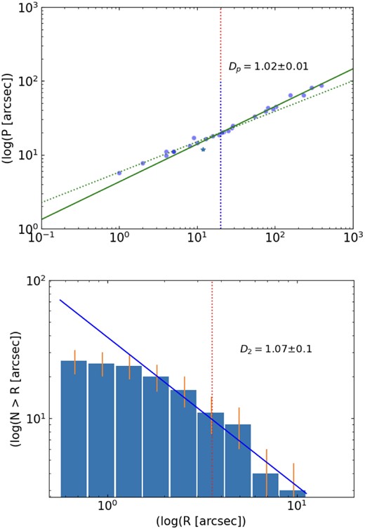
Upper panel shows the perimeter-area relation for structures in the stellar density maps of Fig. 9. Two distinct patterns are discernible. The initial pattern, represented by a dotted line, corresponds to the unresolved component and aligns with the perimeter–area relationship of a circle. The second one, fitted with a continuous green line is the resolved component, which shows a |$D_{P} = 1.02\pm 0.01$| and this result is a clear indication of a fractal dimension. The map’s resolution limit is denoted by the vertical red line. The lower panel presents the histogram that shows the accumulative distribution of the number of the regions, also compatible for the large structures with a fractal regime (|$D_{2} = 1.07\pm 0.1)$|.
Another method to verify this outcome is by examining the relationship |${\rm d}N/{\rm d} \log(R) \propto R^{-D}$| (Mandelbrot 1982; Elmegreen & Falgarone 1996) for the larger groups. The parameter D serves as an additional indicator of a fractal nature, where a value of D < 2 suggests a fractal structure. Applying this correlation to our data set, we obtained a value of |$D _{2}= 1.07 \pm 0.1$|, providing evidence for the fractal attributes in the structure of stellar formation. Grasha et al. (2017) reported similar values |$D_{2}$| = 0.84 for NGC 7793, |$D_{2}$| = 1.6 for NGC 3738, |$D_{2}$| = 1.54 for NGC 6503, and |$D_{2}$| = 1.5 for NGC 1566. However, for NGC 3344 and NGC 628, a more complex situation emerged requiring two lines to fit the results. The findings from NGC 2366 appear to fall within the range observed in the galaxies of the sample studied by Grasha et al. (2017).
6 CONCLUSIONS
We performed an analysis of the young stellar population in the galaxy NGC 2366. Through the PLC method, we found 23 YSGs that could include open clusters, stellar associations, or larger young groups. We found that our sample is complete up to 26 mag. in the filters F555W and F814W having also low photometric errors. This status is supported by a clean CMD that shows the good quality of the observations.
We derived a catalogue that contains the main characteristics of each YSGs, resulting in a mean radius of 16 pc and a minimum radius of 6.19 pc.
Our study of the internal structure of each of the YSGs by means of the Q parameter revealed that the entire sample presents subclumpiness. The average Q value is |$Q_{\rm mean}=0.63 \pm 0.06$| and basically the Q’s for all the YSGs are below 0.8 so they have to be considered as fractal.
We made a surface density map of the blue young stars of the galaxy. Employing the perimeter-area relationship and the cumulative size distribution over this density map, we derived fractal dimensions of |$1.02 \pm 0.01$| and |$1.07 \pm 0.21$|, respectively. These findings align with those observed in other star-forming regions and galaxies, supporting a scenario of hierarchical star formation governed by supersonic turbulence and self-gravity.
ACKNOWLEDGEMENTS
We acknowledge the support from CONICET (PIP 112-202101-00714) and UNLP (I + D 11/G182). This work was based on observations made with the NASA/ESA Hubble Space Telescope, and obtained from the Hubble Legacy Archive, which is a collaboration between the Space Telescope Science Institute (STScI/NASA), the Space Telescope European Coordinating Facility (ST-ECF/ESA), and the Canadian Astronomy Data Centre (CADC/NRC/CSA). Some of the data presented in this paper were obtained from the Mikulski Archive for Space Telescopes (MAST). STScI is operated by the Association of Universities for Research in Astronomy, Inc., under NASA contract NAS5-26555. Support for MAST for non-HST data is provided by the NASA Office of Space Science via grant NNX09AF08G and by other grants and contracts. This research has made use of ‘Aladin sky atlas’ developed at CDS, Strasbourg Observatory, France. We also made use of astrodendro (http://www.dendrograms.org/). The AstroPy python package (Astropy Collaboration et al. 2022) was also utilized for the majority of the calculations performed in this paper.
DATA AVAILABILITY
The original data supporting this article can be accessed at the Space Telescope Institute on the ACS Nearby Galaxy Survey (ANGST) webpage (https://archive.stsci.edu/prepds/angst/). The data for the Young Stellar Groups (YSGs) generated in this study are available in the article.
