


ABSTRACT
We report constraints on a variety of non-standard cosmological models using the full 5-yr photometrically classified type Ia supernova sample from the Dark Energy Survey (DES-SN5YR). Both Akaike Information Criterion (AIC) and Suspiciousness calculations find no strong evidence for or against any of the non-standard models we explore. When combined with external probes, the AIC and Suspiciousness agree that 11 of the 15 models are moderately preferred over Flat-|$\Lambda$|CDM suggesting additional flexibility in our cosmological models may be required beyond the cosmological constant. We also provide a detailed discussion of all cosmological assumptions that appear in the DES supernova cosmology analyses, evaluate their impact, and provide guidance on using the DES Hubble diagram to test non-standard models. An approximate cosmological model, used to perform bias corrections to the data holds the biggest potential for harbouring cosmological assumptions. We show that even if the approximate cosmological model is constructed with a matter density shifted by |$\Delta \Omega _{\rm m}\sim 0.2$| from the true matter density of a simulated data set the bias that arises is subdominant to statistical uncertainties. Nevertheless, we present and validate a methodology to reduce this bias.
1 INTRODUCTION
Our understanding of the Universe fundamentally changed in the late 1990s with the remarkable discovery that the expansion of our Universe is accelerating (Riess et al. 1998; Perlmutter et al. 1999). This discovery established |$\Lambda$|CDM as the standard model of cosmology, which asserts that the Universe at late times is dominated by dark energy in the form of a cosmological constant |$\Lambda$| and cold (non-relativistic), pressure-less dark matter (CDM). However, the nature of dark energy remains a mystery.
In this paper, we use the complete photometrically classified type Ia supernova (SN Ia) data set from the Dark Energy Survey (DES) – which represents the largest, most homogeneous SN data set to date – to assess whether the latest SN Ia data prefers any non-standard cosmological models over |$\Lambda$|CDM.
While |$\Lambda$|CDM fits most data well, it lacks a physical motivation and is currently unable to alleviate tensions between early-time and late-time measurements of parameters such as the current expansion rate of the Universe, |$H_0$| (Aghanim et al. 2020; Riess et al. 2022). These two limitations have led to a wealth of exotic cosmological models being proposed (see Di Valentino et al. 2021, for a review).
Non-standard cosmological models attempt to explain observations in a variety of ways, ideally with some physical justification. Models that mimic the late-time acceleration include dynamical vacuum energy, cosmic fluids, scalar fields as well as modifications to the theory of general relativity. Other models challenge our assumption of large-scale homogeneity and isotropy, and attribute the dimming of distant supernovae to local spatial gradients in the expansion rate and matter density, rather than due to late-time acceleration (Alonso et al. 2010).
Previous analyses have shown that many non-standard models are able to explain the current data (e.g. Davis et al. 2007; Sollerman et al. 2009; Li, Wu & Yu 2011; Hu et al. 2016; Dam, Heinesen & Wiltshire 2017; Zhai et al. 2017; Lovick, Dhawan & Handley 2023), although none have shown strong improvement over |$\Lambda$|CDM. In general non-standard models have only been a good fit to the data if they are able to mimic the expansion history of |$\Lambda$|CDM for some choice of parameters. These analyses conclude that new, more statistically powerful data, across a wide range of cosmological observations are required to discriminate between models.
The DES was designed to provide such data and to reveal in detail both the expansion history and large-scale structure of the Universe. Type Ia supernovae are one of the four pillars of DES science, the others being baryon acoustic oscillations (BAO; DES Collaboration 2024a), galaxy clustering (Pandey et al. 2022; Porredon et al. 2022; Rodríguez-Monroy et al. 2022), and gravitational lensing (Gatti et al. 2021; Amon et al. 2022; Secco et al. 2022).
In this paper we focus on the DES-SN5YR sample (DES Collaboration 2024b) containing 1829 SNe. The DES-SN5YR sample consists of 1635 SNe from the full five years of the DES survey, of which 1499 have a machine learning probability of being a type Ia larger than 50 per cent and range in redshift from 0.10 to 1.13. This is combined with an external sample of 194 spectroscopically confirmed low-z SNe Ia (see Section 6).
Our work builds on previous analyses of non-standard models in two ways. (1) we carefully analyse any cosmological assumptions and approximations that have gone in to the derivation of the information that appears in the Hubble diagram, and estimate their impact. We also provide a prescription for others who would like to use DES SN data to test their own non-standard models, and to provide confidence that there are no hidden assumptions that could bias their result. (2) We constrain a set of non-standard models using the DES-SN5YR sample, with the aim of providing the tightest constraints using SNe Ia measurements alone.
This paper is organized as follows. In Section 2 we describe the cosmology pipeline used to produce a Hubble diagram, focusing on aspects of the pipeline that contain any cosmological model dependence. In Section 3, we introduce a new parameter, |$Q_H$|, that can be used as a single-number to summarize supernova cosmology constraints in the w-|$\Omega _{\rm m}$| plane. This new parameter is useful for testing the impact of the reference cosmology used in our simulated bias corrections in Section 4 and the fiducial cosmology used while determining the standardized magnitudes of SN Ia in Section 5. Section 6 describes the data (SN and other external data sets) that we use in this analysis. In Section 7 we describe the theory behind the cosmological models we test and present our results. We discuss our results in Section 8 and conclude in Section 9.
2 COSMOLOGY PIPELINE
Here, we focus on some areas of the DES-SN5YR baseline analysis described in Vincenzi et al. (2024) – all the way from light curves to cosmology – that are, or may appear to be, subject to cosmological dependencies (highlighted in red in Fig. 1). We aim to provide clarity for others who want to use the DES-SN5YR sample to fit their own models.
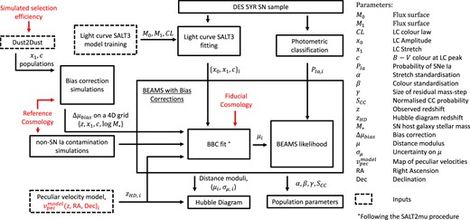
An overview of the light curve to cosmology pipeline. Here, an emphasis is placed on potential cosmological dependencies (red) and the flow of parameters at each stage. Note that we have also omitted parameter uncertainties and the associated covariances for clarity. However, we have included the final uncertainty term, |$\sigma _{\mu , i}$| which includes the intrinsic scatter and a contribution based on the probability of the SN event being a CC contaminant (see Section 2.3.1). A subscript i has been added to SN-dependent parameters. Dashed boxes represent external pippin inputs.
The pipeline, illustrated in Fig. 1, is run within the pippin framework (Hinton & Brout 2020), built around several key components including the salt3 light-curve fitting algorithm (Kenworthy et al. 2021), the superNNova photometric classifier (Möller & de Boissière 2020), snana light-curve fitting, and simulation for bias corrections (Kessler et al. 2009b) producing a bias-corrected Hubble diagram with the ‘Beams with Bias Corrections’ (BBC) formalism (Kessler & Scolnic 2017). We now describe each in turn.
2.1 Light-curve fitting
To convert sparse light-curve observations to SN standardization parameters we use the salt2 model framework (Guy et al. 2007, 2010) as implemented by the salt3 software (Kenworthy et al. 2021). salt3 fits for the time of B-band peak and encapsulates the SN behaviour using three parameters: |$x_0$| is the overall amplitude of the light curve; c is related to the |$B-V$| colour of the SN at peak brightness; and |$x_1$| describes the width of the light curve (stretch). For further details on the light-curve fitting used on the DES-SN5YR sample see Taylor et al. (2023).
The salt3 framework is cosmology independent, except for the assumption that light curves are time-dilated (White et al. 2024) by a factor of |$(1+z_{\rm obs})$|. Note that the observed redshift is used to calculate time dilation, therefore there is no peculiar velocity correction at this stage.
2.2 SN Ia distances
The distance moduli, |$\mu _{{\rm obs},i}$| of SNe Ia are calculated using the modified Tripp equation (Tripp & Branch 1999),
where |$m_{x} = -2.5\text{log}(x_0)$|; |$\mathcal {M}$| is a combination of the SN Ia absolute magnitude, M, and the Hubble constant |$H_0$|, which is marginalized over (see Section 6.3); and |$\alpha$| & |$\beta$| are nuisance parameters that represent the slopes of the stretch–luminosity and colour–luminosity relations, respectively. |$\gamma$| is an additional nuisance parameter that accounts for a correlation between standardized SN luminosities and host-galaxy stellar mass, |$M_{*}$|. This dependence is modelled as a mass-step correction (Conley et al. 2010; Brout et al. 2019). The final term in equation (1), |$\Delta \mu _{\text{bias}}$| is applied to each SN to correct for selection effects.
2.3 BEAMS with bias corrections
The BEAMS with Bias Corrections (BBC; Kessler & Scolnic 2017) framework returns a Hubble diagram from a photometrically1 identified sample of SNe Ia. It does this by maximizing the BEAMS likelihood (Section 2.3.1) that accounts for the probability of the SN event being a core-collapse (CC) contaminant while also incorporating bias corrections (Section 2.3.2) and determining global nuisance parameters, |$\alpha$|, |$\beta$|, and |$\gamma$| from equation (1) (Section 2.3.3). Therefore, along with the Hubble diagram, BBC also outputs the fitted global nuisance parameters, the uncertainty on the estimated distance moduli, |$\sigma _{\mu , i}$|, and a classifier scaling factor that is introduced in Section 2.3.1.
2.3.1 The BEAMS likelihood
Photometric SN samples rely on a classifier to provide a probability of each SN being type Ia or else a contaminant such as core-collapse SN or peculiar SN Ia. The DES-SN5YR baseline analysis uses machine learning techniques to classify SN via the open-source algorithm superNNova (Möller & de Boissière 2020).2 This classification has no cosmological dependence beyond the assumption that the light curves are time dilated by |$(1+z_{{\rm obs},i})$|. The predictions of these classifiers, |$P_{{\rm Ia}, i}$| are incorporated into the cosmology pipeline by using the ‘Bayesian Estimation Applied to Multiple Species’ (BEAMS) approach (Kunz, Bassett & Hlozek 2007; Hlozek et al. 2012; Kunz et al. 2012). The BEAMS approach, involves maximizing the BEAMS likelihood, which includes two terms, one that models the SN Ia population and another that models a population of contaminants. Compared to the traditional likelihood used in spectroscopic samples, the BEAMS likelihood adds one fit parameter, the |$P_{\text{CC}}$| scaling factor |$S_{\text{CC}}$|. The distance uncertainties are then renormalized to ensure that likely contaminants have inflated distance uncertainties and are down-weighted when fitting cosmology. For detailed descriptions of the BEAMS likelihood see Kunz et al. (2012), Kessler & Scolnic (2017), and Vincenzi et al. (2022).
2.3.2 Bias corrections
The BBC approach uses the BEAMS formalism, and estimates the final term in equation (1), |$\Delta \mu _{\text{bias}}$|, using simulations that model the survey detection efficiency, Malmquist bias as well as other biases introduced in the analysis. Simulations of the DES-SN5YR sample are generated using snana3 (Kessler et al. 2019), where light curves are modelled using the salt3 framework and the ‘Dust2Dust’ fitting code (Popovic et al. 2023) measures the underlying population of stretch and colour, including their correlations with host properties.
The simulations used for bias corrections within the baseline analysis are performed using a reference cosmology of Flat-|$\Lambda$|CDM with parameters |$(\Omega _{m},w)_{\text{ref}} = (0.315, -1.0$|). There is an underlying assumption in the BBC framework that the bias correction simulations accurately describe the intrinsic properties of the SNe Ia and selection effects.
The bias correction step thus holds the biggest potential for harbouring cosmological assumptions that could influence the cosmological results. However, the dependence on the reference cosmology has been shown to be weak for models that have similar4 evolution of magnitude versus redshift (Kessler & Scolnic 2017; Brout et al. 2019). Nevertheless, in the analysis of non-standard cosmologies that have the flexibility to deviate significantly from the standard cosmological models, this may no longer be true. In Section 4, we extend on previous work and quantify the cosmological bias resulting from more extreme reference cosmologies in the context of the DES-SN5YR baseline analysis, and provide a prescription for how to fit models that deviate from the reference cosmology significantly in their evolution of magnitude versus redshift.
2.3.3 BBC fit
The global nuisance parameters, |$\alpha$|, |$\beta$|, and |$\gamma$| are used to standardize SN magnitudes and are determined using the BBC fitting algorithm (which has previously been referred to as SALT2mu), following the redshift binning procedure in Marriner et al. (2011) and equation (3) of Kessler & Scolnic (2017). BBC employs a fiducial cosmology5 that provides an arbitrary smooth Hubble diagram in each redshift bin. BBC fits for |$\alpha$|, |$\beta$|, and |$\gamma$| by minimizing the Hubble residuals to the fiducial cosmology among |$N_b=20$| logarithmically spaced redshift bins as well as fitting for a magnitude offset in each bin.
The default fiducial cosmology used in the BBC fit, for the DES-SN5YR analysis, is the Flat-|$\Lambda$|CDM model with parameters |$(H_0, \Omega _{\text{m}}) = (70, 0.3)$|. This choice may cause confusion within the community regarding a potential cosmology dependence. Fig. 2 provides an exaggerated visualization of the BBC fit to show (i) fitting for magnitude offsets in redshift bins allows the data to better resemble its naturally standardized state (with |$\alpha _{\mathrm{fit}}, \beta _{\mathrm{fit}}$| consistent with the true values); (ii) the magnitude offsets (approximately) map the fiducial cosmology on to the true one by quantifying how much the observations deviate from the reference cosmology in each redshift bin; and (iii) that this procedure removes the dependence on cosmological parameters.
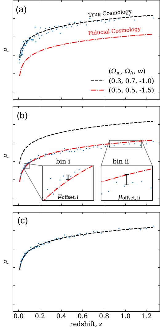
A visualization of the BBC fit. (A) We start with SN distance moduli that are not standardized and therefore have large scatter, here the true cosmology is shown as a black dashed line. BBC employs a fiducial cosmology (red dot-dashed line) that in general is different from the true cosmology. In (B) we then fit for |$\alpha$| and |$\beta$| by minimizing the residual to the fiducial cosmology while simultaneously fitting for magnitude offsets in |$N_b=20$| logarithmically spaced redshift bins. The insets show the varying size of the offsets in different bins relative to the average offset, |$\mu _{\mathrm{offset, }b} = \Delta \mu _b-\mu _{\mathrm{avg}}$|. As |$\mu _{\mathrm{offset, i}}$| does not in general equal |$\mu _{\mathrm{offset, ii}}$| this procedure allows the data to better resemble the true cosmology (black dashed line) approximately mapping the fiducial cosmology on to the true one by quantifying how much the observations deviate from the fiducial cosmology in each redshift bin. In (B), the data has been shifted to the fiducial cosmology for illustrative purposes and in (C) we shift the data back. Therefore, for this example, |$\mu _{\mathrm{avg}}$| would be positive (the data actually sits above our fiducial cosmology), however |$\mu _{\mathrm{offset, }i}$| and |$\mu _{\mathrm{offset, }ii}$| would be positive and negative, respectively (because the data sits above and below the average offset, respectively). While this example is exaggerated it is useful to provide insight into BBC and highlight that the method has minimal cosmological dependence.
Marriner et al. (2011) show that the fit for |$\alpha$| and |$\beta$| is decoupled from the choice of fiducial cosmology if the number of redshift bins is sufficiently large. Furthermore, Kessler, Vincenzi & Armstrong (2023) performs a limited study that looks at the standard deviation of the Hubble residuals of the BBC fit (see table 1 of Kessler et al. 2023). In Section 5, we re-test this result and extend on the work of Marriner et al. (2011) and Kessler et al. (2023) by explicitly testing extreme cosmologies as well as showing that the impact on cosmology-fitted parameters is negligible. Finally, we present an alternate approach that does not require a fiducial cosmology and achieves consistent fits for |$\alpha$| and |$\beta$|.
2.3.4 SN Ia distance uncertainties
Following the Pantheon + analysis (Brout et al. 2022), the distance modulus uncertainties |$\sigma _{\mu ,i}$| are calculated within the BBC approach as,
where |$\sigma _{\mathrm{S3fit},i}$| includes the uncertainties on the light-curve parameters and the associated covariances; while |$\sigma _{\mathrm{lens},i}$| and |$\sigma _{z,i}$| are uncertainties associated with lensing effects and spectroscopic redshifts, respectively. |$f(z_i, c_i, M_{*,i})$| and |$\sigma _{\mathrm{floor}}(z_i, c_i, M_{*,i})$| are survey-specific scaling and additive factors that are estimated from the BBC simulations. Finally, |$\sigma _{{\rm vpec},i}$| accounts for uncertainties due to peculiar velocities, including both uncertainties in linear-theory modelling and non-linear unmodelled peculiar velocities, as discussed in Section 2.4.
2.4 Modelling peculiar velocities
The redshift that is compared to SN distances should be entirely due to the expansion of the universe. However, in practice the redshift that we measure contains contributions due to peculiar velocities of the SN and its host galaxy. The DES-SN5YR baseline analysis uses peculiar velocities presented by Peterson et al. (2022), which are determined from the 2M+ + density fields (Carrick et al. 2015) with global parameters and group velocities used from Said et al. (2020) and Tully (2015), respectively, and a 240 km s|$^{-1}$| uncertainty on these estimates. While the determination of the peculiar velocity corrections includes a fiducial cosmology, the corrections have the largest impact at low redshifts where the cosmology dependence is negligible. Although Peterson et al. (2022) show that the impact of peculiar velocity corrections on |$H_0$| and w fits are at the 1 per cent level, the impact of the fiducial cosmology in the derivation of those corrections is negligible compared to the uncertainty in the peculiar velocity map, and therefore we do not consider it further in this work.
3 The |$\Omega _{\mathrm{m}}-w$| degeneracy
There is a degeneracy between the equation of state of dark energy and the matter content of the universe for distance indicators within generalized dark energy models. It has long been known that this degeneracy makes it more difficult to assess systematics on |$\Omega _{\rm m}$| and w separately.
Large shifts in the best-fitting parameters may not be significant if they occur along the degeneracy direction, but the same size shifts could be very significant if they occur perpendicular to the degeneracy direction. In the DES cosmology analysis we use two methods to account for that degeneracy. The first is setting a prior on matter density6 and only considering changes in w, the other is testing a new parameter |$Q_H(z)$| that allows us to present a single non-degenerate number summarizing a SN Ia constraint in the w-|$\Omega _{\rm m}$| plane.
To link Flat-wCDM and cosmography, we can use the acceleration equation
where |$\Omega _{\rm de} = 1-\Omega _{\mathrm{m}}$| for a spatially flat universe. Note that |$H\equiv \dot{a}/a$|, therefore using the definition of the deceleration parameter, |$q\equiv -\ddot{a}/(a H^2)$| we can rearrange equation (3) and express |$q(H/H_0)^2$| as a function of the energy mix of a Flat-wCDM universe,
where we have defined |$Q_H\equiv -\ddot{a}/(aH_0^2)\equiv q(H/H_0)^2$| and |$a = (1+z)^{-1}$|.
In Fig. 3 we show lines of constant |$Q_H(z)$| overlaid on to the |$1\sigma$| and |$2\sigma$| contours for the DES-SN5YR sample. Since the |$Q_H(z)$| parameter is redshift dependent, it is not as universal as a parameter such as |$S_8=\sigma _8\sqrt{\Omega _{\rm m}/0.3}$|, which defines a quantity that is relatively independent of the |$\sigma _8$| and |$\Omega _{\rm m}$| degeneracy in lensing studies. Instead, we can select a redshift that matches the degeneracy direction of the sample. In the top right subplot of Fig. 3 we show that |$Q_H(0.2)$| makes a good approximation for the w-|$\Omega _{\rm m}$| degeneracy line for the DES-SN5YR sample. Using the |$Q_H(0.2)$| parameter, we can therefore use a single number to approximate the DES-SN5YR constraints on the Flat-wCDM model and find |$Q_H(0.2)=-0.340\pm 0.032$| (which includes statistical and systematic uncertainties).
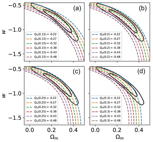
Comparing lines of constant |$Q_H(z)$| with |$z = 0.15, 0.20, 0.25, 0.30$| for panels (a), (b), (c), (d), respectively. Here, we overlay in each panel the Flat-wCDM |$1\sigma$| and |$2\sigma$| contours for the DES-SN5YR sample.
Changes to the analysis that only cause shifts along the degeneracy direction have a very small effect on |$Q_H$| even though they can have a misleadingly large effect on |$\Omega _{\rm m}$| and w (misleading since those shifts are strongly correlated). |$Q_H$| is thus an excellent measure by which to evaluate the impact of analysis choices on the supernova cosmology results (see Fig. 4).
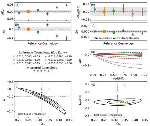
(a) and (b): Shifts in |$\Omega _{\mathrm{m}}$| and w (solid points) when using different BBC simulations that are distinguished by a unique reference cosmology (shown by open symbols; listed in the figure legend). The shifts are measured relative to the perfect scenario (orange square) where the reference cosmology is equal to the true cosmology of our simulated data. (c) and (d): The associated mean shifts in |$Q_H(0.20)$| (with no prior) as well as w determined with a strong prior on the matter density of |$\Omega _{\mathrm{m}}=\Omega _{\mathrm{m, true}}\pm 0.001$|, which minimizes the impact that the |$\Omega _{\mathrm{m}}-w$| degeneracy has on investigating the BBC reference cosmology. For panels (a)–(d) we have averaged over 25 DES-SN5YR simulations. Note also that the error bars show the uncertainty on the shift in the mean – not the uncertainty on the parameters, which is larger. (e): Calculated residual distance moduli of the reference cosmologies (dashed lines) relative to the baseline cosmology |$(\Omega _{\mathrm{m}}, w) = (0.315,-1.0)$| in orange. The solid lines represent the variation in the expansion history from the perfect scenario using the mean of the best-fitting parameters. (f): Best-fitting parameters (solid points) for 1 realization of simulated data determined using a unique BBC reference cosmology (shown by open symbols). The |$1\sigma$| and |$2\sigma$| contours shown are for the ideal case (orange square). The grey dotted dashed line represents the |$Q_H(0.2)$| parameter. (g): Equivalent information to that contained in plot (f) but converted to |$\Omega _{\mathrm{m}}-Q_H(0.2)$| space.
4 REFERENCE COSMOLOGY IN THE BIAS CORRECTION SIMULATIONS
Kessler & Scolnic (2017) show that any dependence on the reference cosmology is weak when the reference cosmology is similar to the true evolution of magnitude versus redshift (see section 6.1 and fig. 7 of Kessler & Scolnic 2017, for details). Here, we reevaluate this systematic and also show that using a reference cosmology even |$10\sigma$| away from the true cosmology has less than a |$1\sigma$| shift in the results. We also present an iterative method that can be used to reduce even that small systematic offset.
4.1 Testing the impact of the reference cosmology
To examine the impact that the reference cosmology used for the bias correction simulations has on our cosmology fits, we generate and analyse 25 realizations of simulated data. These are created with a Flat-wCDM cosmology with parameters |$(H_0, \Omega _{\mathrm{m}}, w) = (70,0.315,-1.0)$|. We also generate six different BBC simulations, each with a unique reference cosmology. For comparison, in Fig. 4(e) we plot each reference cosmology (dashed lines) relative to the cosmology used to generate our simulated data (orange).
The average shifts in |$\Omega _{\mathrm{m}}$| and w from the perfect scenario in which the reference cosmology is equal to the true cosmology of our simulated data are shown in Figs 4(a) and (b), respectively.7
In Fig. 4(f) we plot the results in the |$w-\Omega _{\rm m}$| plane for a single realization. The contours and solid orange square are for the ideal case in which the reference cosmology matches the true cosmology. The other symbols show the results when using different reference cosmologies, where the open symbols show the input reference cosmology and the solid symbols show the resulting best-fitting parameters.
This shows that while the shifts in |$\Omega _{\rm m}$| and w seem large, when viewed in 2D parameter space they all fall along the |$\Omega _{\mathrm{m}}-w$| degeneracy direction and are thus all well within |$1\sigma$|.
The dot-dashed line in Fig. 4(f) shows the |$Q_H(0.2)$| parameter, representing the degeneracy line. Note that the ideal redshift for |$Q_H$| to match the degeneracy direction will change depending on the data set. In Fig. 4(c) we plot the average shift in |$Q_H(0.2)$| and in Fig. 4(d) we plot the shift in w after applying a strong prior on the matter density |$\Omega _{\mathrm{m}}=\Omega _{\mathrm{m, true}}\pm 0.001$|. The fact that the shifts in |$Q_H(0.2)$| and |$w|_{\Omega _{\mathrm{m, true}}\pm 0.001}$| are negligible shows that the impact of the reference cosmology is small and limited to the degeneracy direction, in agreement with the results from Kessler & Scolnic (2017).
We also performed two additional tests that are the inverse of those performed above. Instead of varying the reference cosmology, we fixed the reference cosmology to the baseline cosmology used in the DES-SN5YR analysis and generated 25 realizations of simulated data using both (a) Flat-wCDM cosmology with parameters |$(H_0, \Omega _{\mathrm{m}}, w) = (70,0.350,-0.8)$| and (b) Flat-|$w_0 w_a$|CDM cosmology with parameters |$(H_0, \Omega _{\mathrm{m}}, w_0, w_a) = (70,0.495,-0.36, -8.8)$|. These cosmologies were chosen to match the |$\sim 10\sigma$| offset brown point in Fig. 4 and the best fit Flat-|$w_0 w_a$|CDM result in the DES-SN5YR analysis, respectively. The results are given in Table 1. For test (a), we again find that the impact of using the incorrect reference cosmology is negligible. For test (b), we see larger shifts in cosmological parameters. However, in this case, there is an additional degeneracy between |$w_0-w_a$| that is not accounted for when applying the prior on |$\Omega _{\mathrm{m}}$|. To visualize this, we plot the 25 realizations in Fig. 5 which shows that the best-fitting points are aligned along the degeneracy line and consistent with the truth. We also note that the uncertainties given in Table 1 are on the shift in the mean. The shifts are |$\Delta w_0 = 0.18\pm 0.28$|, |$\Delta w_a = -1.6\pm 2.2$| when using the uncertainty on the parameters.
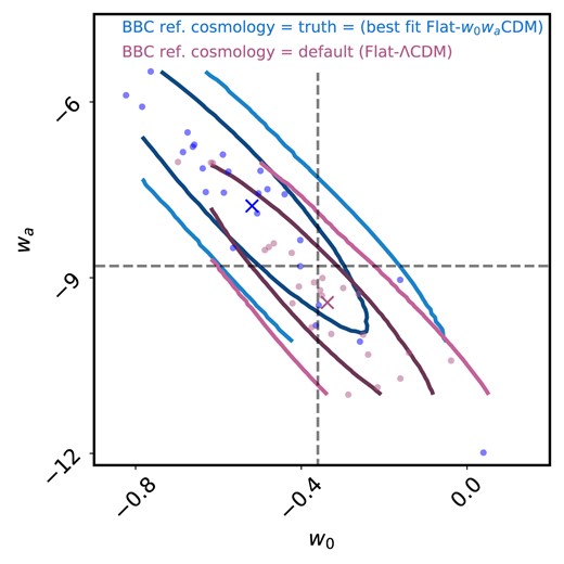
Comparison of the best fit |$w_0-w_a$| points (with a prior on the matter density, |$\Omega _{\mathrm{m}}=\Omega _{\mathrm{m, true}}\pm 0.001$|) determined using the DES-SN5YR baseline reference cosmology (purple) and when the reference cosmology is set to the input cosmology of the simulations (blue). The points show the maximum-likelihood values for each realization and the crosses represent the averages of the those maximum-likelihood values. The ellipses are the 1- and 2|$\sigma$| contours representing the dispersion of best-fitting points.
Shifts in the best-fitting parameters using the DES-SN5YR baseline reference cosmology, from the perfect scenario where the reference cosmology is equal to the cosmology used to generate the simulated data. Here, the uncertainties are on the shift in the mean – not the uncertainty on the parameters, which is larger.
| Model|$^{*}$| | |||
|---|---|---|---|
| (|$\Omega _{\mathrm{m}}$|, |$w_0$|, |$w_a$|) | |$\Delta Q_\mathrm{H}(0.20)$| | |$\Delta w_0^{\dagger }$| | |$\Delta w_a^{\dagger }$| |
| |$(0.350, -0.80, 0)$| | |$0.02 \pm 0.05$| | |$0.000 \pm 0.008$| | – |
| |$(0.495, -0.36, -8.8)$| | – | |$0.18\pm 0.06$| | |$-1.6\pm 0.4$| |
Notes.|$^{*}$|Model used to generate the 25 realizations of simulated data.
|$^{\dagger }$|Determined used a prior on the matter density of |$\Omega _{\mathrm{m}}=\Omega _{\mathrm{m, true}}\pm 0.001$|.
In summary, this result validates that the BBC baseline approach used in DES Collaboration (2024b) is able to return a Hubble diagram that represents the true distance versus redshift relation to within |$1\sigma$| even given a reference cosmology that is |$\sim 10\sigma$| from the truth (brown point in Fig. 4) or varies by |$\sim \Delta \mu = 0.15$| (brown dashed line in Fig. 4e). The apparent bias observed in Figs 4(a) and (b) is due to showing shifts in degenerate parameters separately, without considering the combined influence on the distance versus redshift relation. Importantly, we can be confident in our bias corrections if the expansion history of a non-standard cosmological model falls within the region bounded by the blue and brown dashed lines in Fig. 4(e).
4.2 The iterative method
Section 4.1 validates the procedure used in the DES-SN5YR baseline analysis, showing that the reference cosmology has a small impact on the cosmological results relative to the statistical uncertainties. However, the BBC reference cosmology may become a dominating systematic for future surveys such as the Rubin Observatory’s LSST, which will include hundreds of thousands of well measured SNe Ia (LSST Science Collaboration 2009). Furthermore, Fig. 4 shows that in the case where one finds a tension with other data sets at the extreme ends of the degeneracy direction (e.g. if the CMB contours were at the top left or bottom right in Fig. 4f), it would be beneficial to ensure a close match to the reference cosmology. Since we performed a blind analysis, we did not know whether there would be a discrepancy between the BBC reference cosmology and the final fitted cosmology results. We therefore prepared the following method to correct the reference cosmology if the discrepancy was significant.
It was suggested by Kessler & Scolnic (2017) that an iterative procedure can be applied where |$w_{\text{ref}}$| is updated with the previous |$w_{\text{fit}}$| value, to reduce this bias. This procedure is summarized in Fig. 6. In this work, we test the iterative method by applying it to 10 realizations of simulated data created with a Flat-wCDM cosmology with parameters |$(H_0, \Omega _{\mathrm{m}}, w)=(70, 0.350, -0.8)$|. This cosmology was selected due to its location in parameter space, which is approximately perpendicular to the |$\Omega _{\mathrm{m}}-w$| degeneracy line in the direction of a general CMB prior and lies outside a |$2\sigma$| region (based on DES-SN5YR simulations) of the default BBC reference cosmology.8 Table 2 shows the weighted average shift in cosmological parameters from the truth after 10 realizations. Note that the |$\Omega _{\mathrm{m}}$| prior was only applied on our final results and was not used during the iterative process. We report both |$\Delta w|_{\Omega _{\mathrm{m, true}}\pm 0.001}$| and |$\Delta Q_H(0.2)$| and find that both are closer to the truth after applying the iterative method. In particular, we find that |$w|_{\Omega _{\mathrm{m, true}}\pm 0.001}$| has shifted by 0.006 and |$Q_H(0.2)$| has shifted by 0.008 closer to the truth.
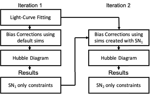
Iterative procedure methodology. During the first iteration, bias corrections are modelled using simulations created using the default reference cosmology with a fixed set of Flat-wCDM parameters |$\Omega _{\mathrm{m},\text{ref}} = 0.3$| and |$w_{\text{ref}} = -1.0$|. In the second iteration, the simulations are instead created using the maximum-likelihood estimates from the first iteration.
Testing the iterative method (Section 4.2): Weighted average (over 10 realizations|$^{*}$|) difference in w and |$Q_H$| from the truth for the first and second iterations.
| Method | |$\Delta w^{\dagger }_{\mathrm{fit-true}}$| | |$\sigma _{w\mathrm{, avg}}$| | |$\Delta Q_\mathrm{H, fit-true}$| | |$\sigma _{Q_\mathrm{H, avg}}$| |
|---|---|---|---|---|
| Nominal | |$-$|0.023 | 0.028 | |$-$|0.051 | 0.019 |
| |$2^{\mathrm{nd}}$| Iteration | |$-$|0.017 | 0.025 | |$-$|0.043 | 0.019 |
Notes.|$^{*} \Omega _{\mathrm{m}}=0.350$| and |$w=-0.8$| was used as the true cosmology.
|$^{\dagger }$| With a prior on the matter density of |$\Omega _{\mathrm{m}}=0.350\pm 0.001$|.
We note a limitation of this work that we have not explicitly shown the iterative method converges (because repeatedly redoing the simulations is computationally intensive). However, we performed a third iteration on two random realizations and found that the iterative method remained stable.
The iterative method was not implemented in the current DES results, because after unblinding we found the best-fitting cosmology to be sufficiently close to the reference cosmology so as to make any bias insignificant (in Section 4.1 we found |$\Delta w \sim 0.01$| given a reference cosmology 10|$\sigma$| from the truth). Nevertheless, we conclude that iterating the reference cosmology is a viable method to reduce this bias for future analyses where the reference cosmology may become a dominating systematic.
5 TESTS OF COSMOLOGY DEPENDENCE WITHIN THE BBC FIT
In this section, we validate the baseline analysis assumption that the fit for nuisance parameters is decoupled from the choice of fiducial cosmology using 20 logarithmically space redshift bins (for these tests we restrict ourselves to |$\alpha$| and |$\beta$|).
In total, we generated 100 statistically independent realizations that resemble the DES-SN5YR sample in a spatially Flat-|$\Lambda$|CDM universe with parameters |$(H_0, M_B, \Omega _{\mathrm{m}}) = (70, -19.253, 0.3)$|. We ran all 100 realizations through the entire PIPPIN pipeline six times with each run distinguished uniquely by the choice of fiducial cosmology within the BBC fitting procedure. The choice of fiducial cosmologies was chosen such that they vary significantly in the evolution of magnitude versus redshift and are shown in the bottom panel of Fig. 7.
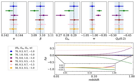
Top panels: Shifts in the average maximum likelihood |$\alpha$|, |$\beta$|, |$\Omega _{\mathrm{m}}$|, w, and |$Q_H(0.2)$| values after varying the fiducial cosmology within the BBC fit (Section 5). The error bars used are the standard error of the mean and are therefore much larger for the individual case. The values are shown relative to the ideal case (black dashed line) where the fiducial cosmology is equal to the true cosmology used to simulate the data. Only the model with zero matter density, and pure cosmological constant (plum) shows a more than |$1\sigma$| shift from the fiducial, and comparison with both the |$Q_H$| panel and Fig. 8 shows that shift is along the degeneracy direction. Bottom right: Variation in the evolution of magnitude versus redshift from the ideal case for (a) the input fiducial cosmological parameters (given in the legend) shown as dashed lines and (b) using the mean of the best-fitting parameter values shown in the zoomed inset axes as solid lines.
The left panel of Fig. 8 compares the maximum likelihood |$\alpha$| and |$\beta$| values for each of the 100 realizations. The top left sub-plot represents the ideal case where the fiducial cosmology is equal to the true cosmology used to simulate the data. Here, we show how the averages of the 100 maximum-likelihood values (blue crosses) compared to the true values (black dashed lines). We also make the equivalent comparison after fitting for cosmological parameters, shown in the right panel of Fig. 8. In Fig. 7 we present the shifts in the average of the maximum likelihood |$\alpha$|, |$\beta$|, |$\Omega _{\mathrm{m}}$|, w, and |$Q_H(0.20)$| values as a result of varying the fiducial cosmologies within the BBC fit. We also show how the shifts in cosmological parameters impacts the evolution of magnitude versus redshift relative to the ideal case.
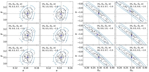
Left: The best fit |$\alpha$| and |$\beta$| for 100 mock realizations for each of six different reference cosmologies as per the legend (see Section 5). The black points show the maximum-likelihood values for each realization and the blue crosses represents the averages of the those maximum-likelihood values. The blue ellipses are the 1- and 2|$\sigma$| contours representing the dispersion of best-fitting points. The upper left sub-figure represents the perfect scenario where the fiducial cosmology is equal to the true cosmology used to simulate the data. The black dashed lines are used to compare each figure to this ideal case. Right: The equivalent figure after fitting for cosmological parameters, |$\Omega _{\mathrm{m}}$| and w.
We find that the determination of the global nuisance parameters, |$\alpha$| and |$\beta$|, has a weak dependence on the choice of fiducial cosmology; these results are in agreement with those by Marriner et al. (2011). Extending on the work by Marriner et al. (2011), Fig. 7 shows that the BBC fit is able to recover the ideal cosmological parameters with less than a |$1\sigma$| tension of the standard error given 100 realizations even when using extreme fiducial cosmologies. The two fiducial cosmologies that result in the largest shift in cosmological parameters are unsurprisingly also the two cosmologies that deviate the most in the slope of the distance versus redshift relation |$(H_0, \Omega _{\mathrm{m}}, \Omega _{\Lambda }, w)=(70, 0.0, 1.0, -1.0)$| and |$(70, 1.0, 0.0, -1.0)$|. However, both the |$Q_H(0.2)$| panel and Fig. 8 show that shift is along the degeneracy direction.
Finally, the lower right of Fig. 7 shows the μ differences between the fiducial cosmologies (dashed lines) and even shifts of μ up to 0.5 across the z-range have negligible impact on the best-fitting expansion history (solid lines).
5.1 Is a fiducial cosmology required?
Often, the role of the fiducial cosmology within the BBC fit causes confusion – both because of perceived cosmology dependence (which we have shown is negligible for any reasonable cosmology in Section 5) and because it is mistaken for the reference cosmology used to generate the BBC simulations that estimates the |$\mu _{\mathrm{bias}}$| term in equation (1).
Here, we explore replacing the fiducial cosmology (along with the fitted magnitude offsets in each bin) within the BBC fit with a spline interpolation of the SN magnitudes. To accomplish this, we modify the BBC procedure. Recall that within the current BBC procedure the Hubble residuals are minimized to a fiducial cosmology among 20 independent redshift bins, given a set of global nuisance parameters and 20 offsets in magnitude. Here, we instead minimize the Hubble residuals to a spline interpolation of the SN magnitudes, determined at each fitting step, where we used the weighted average redshift, |$z_{\mathrm{avg}}$| and distance moduli, |$\mu _{\mathrm{avg}}$| in 20 redshift bins as knots.
We compare these two procedures by recreating a simplified BBC fitting procedure that attributes all of the intrinsic scatter to coherent variation at all epochs and wavelengths, |$\sigma _{\rm int}$|.9 Further complexity is not required as the intrinsic scatter is incorporated into the uncertainties in the same way if we use a fiducial cosmology or a spline and we only need to test consistency between the two methods.10
Table 3 compares the fitted nuisance parameters using the same light-curve sample when using two different fiducial cosmologies (see Table 3 for model parameters) and a spline that is determined at each fitting step. All parameters are consistent demonstrating the following. First, that the results from our simplified BBC fit are again insensitive to the choice of fiducial cosmology. Secondly, that a spline is viable alternative to a fiducial cosmology and may reduce confusion as to the role of the fiducial cosmology in future pipelines.
BBC fitted nuisance parameters for three different fiducial cosmologies, showing the results are stable to the choice of fiducial cosmology or use of a spline (see Section 5.1).
| Fiducial cosmology | |||
|---|---|---|---|
| Parameters | Flat-|$\Lambda$|CDM|$^\dagger$| | Flat-wCDM|$^{*}$| | Spline |
| |$\sigma _{\mathrm{int}}$| | |$0.095^{+0.003}_{-0.004}$| | |$0.098\pm 0.004$| | |$0.099^{+0.003}_{-0.004}$| |
| |$\alpha$| | |$0.136\pm 0.004$| | |$0.136^{+0.004}_{-0.005}$| | |$0.137\pm 0.004$| |
| |$\beta$| | |$3.008^{+0.040}_{-0.047}$| | |$2.958^{+0.039}_{-0.048}$| | |$2.978^{+0.040}_{-0.051}$| |
Notes.|$^{\dagger }(H_0,\Omega _{\mathrm{m}}) =(70, 0.3)$|
|$^{*}(H_0,\Omega _{\mathrm{m}}, w) =(60, 0.4, -0.8)$|
6 DATA
Having established that the derivation of the DES-SN5YR Hubble diagram is robust to the choice of reference and fiducial cosmological models, we turn to using the Hubble diagram to derive constraints on a range of non-standard models which differ in their background expansion and are therefore sensitive to the DES-SN5YR data. To test the non-standard cosmology fitting code, we generated 25 simulations and ensured that fitted parameters of each model were consistent with the input cosmology. The input cosmology for these simulations used Flat-|$\Lambda$|CDM, for models that could reduce to Flat-|$\Lambda$|CDM for some values of their parameters. Otherwise, we used the model being tested as the input cosmology to generate the 25 realizations.
6.1 The DES-SN5YR sample
The DES-SN survey covers |$\sim$|27 deg|$^2$| over 10 fields across the DES footprint (see Smith et al. 2020). The survey, which ran for five years using the Dark Energy Camera (DECam; Flaugher et al. 2015). DES detected over 30 000 SN candidates, from these 1635 were deemed SNe Ia-like and included in the DES-SN5YR Hubble diagram with 1499 photometrically classified as type Ia SNe using superNNova (Müller et al. 2022; Vincenzi et al. 2024). The DES-SN5YR sample includes publicly available low-z SNe Ia from the Harvard-Smithsonian Center for Astrophysics, CfA3 (Hicken et al. 2009) and CfA4 (Hicken et al. 2012), the Carnegie Supernova Project, CSP (Krisciunas et al. 2017) and the Foundation Supernova Survey (Foley et al. 2018). These low-z samples span a redshift range of 0.01 to 0.1. However, SNe Ia in the low-z sample with redshifts |$\lt 0.025$| are excluded to minimize the impact of peculiar velocities. With this cut applied, the low-z sample comprises 194 SNe, for a total of 1829 SNe in the DES-SN5YR sample; for more details see Müller et al. (2022), Vincenzi et al. (2024), and Sánchez et al. (2024).
6.2 External probes
Our data must be interpretable in context of the parameters of the cosmological models that we test. In this work, many of these are defined as modifications to the background expansion and do not describe how the CMB or galaxy power spectrum may change. Additionally, we would like to be agnostic about the pre-recombination history, and in particular the size of the sound horizon |$r_d$| or |$r_*$|.
Fortunately, as we describe below, we may still combine the DES-SN5YR cosmological constraints with measurements based on observations from the Cosmic Microwave Background (CMB) and Baryon Acoustic Oscillations (BAO) by the use of derived parameters with clear physical meaning. We do not use data from weak lensing surveys in this work.
6.2.1 Cosmic microwave background
The CMB data may be expressed in terms of the ‘shift parameter’ R (Bond, Efstathiou & Tegmark 1997), defined in the literature as
where |$z_*$| is the redshift at the surface of last-scattering, |$E(z)\equiv H(z)/H_0$| is the normalized redshift-dependent expansion rate and
The physical meaning of R in the context of non-standard cosmological models may be understood if the baryon density |$\omega _b = \Omega _b h^2$| is fixed (for example by nucleosynthesis constraints). Although R is sometimes interpreted as set by the location of the peaks and troughs of the CMB power spectrum (if the sound speed is fixed by |$\omega _b$| and |$T_{\rm CMB}$|), this relies on the absence of additional energy components in the pre-combination era (for example, early dark energy models as reviewed in Poulin, Smith & Karwal 2023). Alternatively, R may also be understood as localized around the surface of last scattering in the following way. During recombination, photons stream out of overdensities and suppress power on small scales in a process known as Silk damping (Silk 1968). Again at fixed |$\omega _b$|, successive spectral peaks are lower than their predecessors as the multipole l increases, and the rate of suppression |$C_l \propto \exp {-2(l/l_{\rm Silk})^2}$| (see for example, Mukhanov 2004) is proportional to the Hubble expansion rate at the time of last scattering. We may therefore define
where |$D_M(z)$| is the transverse comoving distance defined as
We see that |$R^{\prime } \simeq R$| provided the universe is matter-dominated at the time of last scattering. It may be calculated that |$R^{\prime } \simeq 1.8 \times 10^{-3} l_{\rm Silk}$| where the prefactor is only sensitive to cosmological parameters by a factor of |$(1+z_*)^{1/2}$| and in turn |$z_*$| does not depend much on the cosmology. Hence |$R^{\prime }$|, which is explicitly proportional to |$H(z_*)$|, connects R to the Silk damping scale which we take as a safe assumption for the range of models we test.
Chen, Huang & Wang (2019) converted the Planck 2018 (Aghanim et al. 2020) TT, TE, EE+lowE measurements to a prior on R, finding |$R=1.7502\pm 0.0046$| for models assuming spatial flatness and |$R=1.7429\pm 0.0051$| for models that allow curvature. We use these priors in this work. We also note that Lemos & Lewis (2023) remove late-time cosmology dependence from the CMB likelihoods by using flexible templates for late-ISW and CMB-lensing. We convert their baseline results (Early-|$\Lambda$|CDM, see table 1 of Lemos & Lewis 2023) into a constraint on the shift parameter and find |$R=1.7442\pm 0.0044$|. Reassuringly, the central value falls between the constraints from Chen et al. (2019).
6.2.2 Baryon acoustic oscillations
Baryon acoustic oscillations represent a sharply defined acoustic angular scale on the sky given by
where |$D_M(z_d)$| is the transverse comoving distance to the drag epoch, and |$r_d$| is the comoving sound horizon given by
and |$c_{s}$| is the baryon sound speed, while |$r_{*}$| and |$\theta _*$| are defined in the same way using |$z_*$|.
BAO measurements are given as the ratio of |$r_d$| to either the Hubble distance, |$D_H(z)=c/H(z)$|, transverse comoving distance, |$D_M(z)$|, or a combination of the two termed the dilation scale, |$D_V(z) \equiv \left[z D_M^2(z) D_H(z)\right]^{1/3}$|. To interpret these in terms of distances, |$r_d$| is needed. However, in this work, we cancel the dependence on the sound horizon scale by using the ratio of the BAO distance with the distance to CMB as,
where |$D_{X_i}=$| {|$D_{V}$|, |$D_{M}$|, |$D_{H}$|}, and we remind the reader that |$D_{M}(z_*) = (c/H_0) R/\sqrt{\Omega _m}$|. In this way, the data represents the ratio of the angular scales of the sound horizon on the surface of last scattering and at the effective redshift of the BAO. The cosmological dependence of |$r_*/r_d$| may be neglected.
We use BAO data from the extended Baryon Oscillation Spectroscopic Survey (eBOSS; Dawson et al. 2016; Alam et al. 2021), which is the cosmological survey within SDSS-IV (Blanton et al. 2017). Specifically, we use the BAO-only measurements from SDSS MGS (Ross et al. 2015), SDSS BOSS (Alam et al. 2017), SDSS eBOSS LRG (Bautista et al. 2021), SDSS eBOSS ELG (de Mattia et al. 2021), SDSS eBOSS QSO (Hou et al. 2021), and SDSS eBOSS Ly |$\alpha$| (du Mas des Bourboux et al. 2020). We note that new BAO measurements from both DES (DES Collaboration 2024a) and the DESI collaboration (DESI Collaboration 2024) were released in the advanced stages of this work and motivates a follow-up analysis with the inclusion of these data sets.
The covariance matrices provided by eBOSS11 have been incorporated into this study with the use of the uncertainties (Lebigot 2009) python package and the final measurements shown in Table 4. Note that although these measurements contain information from the CMB we will refer to these measurements as BAO-|$\theta _*$| from here on.
Summary of the external constraints determined using measurements from eBOSS and Planck.
| BAO-|$\theta _*$| measurements|$^{*}$| | |||
|---|---|---|---|
| |$z_{\text{eff}}$| | |$D_M(z_*)/D_V(z)$| | |$D_M(z_*)/D_M(z)$| | |$D_M(z_*)/D_H(z)$| |
| 0.15 | |$21.13 \pm 0.80$| | – | – |
| 0.38 | – | |$9.22 \pm 0.15$| | |$3.78 \pm 0.11$| |
| 0.51 | – | |$7.06 \pm 0.11$| | |$4.23 \pm 0.11$| |
| 0.70 | – | |$5.28 \pm 0.10$| | |$4.88 \pm 0.14$| |
| 0.85 | |$5.15 \pm 0.25$| | – | – |
| 1.48 | – | |$3.07 \pm 0.08$| | |$7.12 \pm 0.30$| |
| 2.33 | – | |$2.52 \pm 0.13$| | |$10.58 \pm 0.34$| |
| 2.33 | – | |$2.52 \pm 0.11$| | |$10.42 \pm 0.36$| |
| CMB-R measurements|$^\dagger$| | |||
| |$z_*$| | |$\Omega _{\rm k}$| | R | |
| 1089.95 | |$=0$| | |$1.7502\pm 0.0046$| | |
| 1089.46 | |$\ne 0$| | |$1.7429\pm 0.0051$| | |
Notes.|$^{*}$| The product of the BAO measurements with the CMB acoustic scale.
|$^{\dagger }$| In this work we use the ‘shift parameter’ R that is related to the heights of the CMB acoustic peaks and depend on the line-of-sight distance to the sound horizon.
6.3 Constraining cosmological models
In general, the parameters of an individual cosmological model are constrained by minimizing a |$\chi ^2$| likelihood given by
and for DES-SN5YR, |$D_i = \mu _{\text{model},i}-\mu _i$| for the |$i^{th}$| SN. However, the absolute magnitudes of SNe Ia are degenerate with |$H_0$|. For this analysis, no assumption on |$H_0$| is presumed and instead |$H_0$| is treated as a nuisance parameter that is analytically marginalized over by modifying equation (12). The modified |$\chi ^2$| likelihood is given by (Goliath et al. 2001),
where
and
and where we sum over all matrix elements, |$i,j$|. For the combined constraints we sum the |$\chi ^2$| likelihoods from all data sets as
cobaya12 (Torrado & Lewis 2019; Torrado & Lewis 2021), a robust code for Bayesian analysis, was used to minimize equations (13) and (16). The convergence of MCMC chains was assessed in terms of a generalized version of the |$R-1$| Gelman-Rubin statistic (Gelman & Rubin 1992), which measures the variance between the means of the different chains in units of the covariance of the chains. For our work, we adopted a more stringent tolerance than cobaya’s default value, namely |$R-1=0.001$|.
7 COSMOLOGICAL MODELS AND RESULTS
DES Collaboration (2024b) presents cosmological results for the standard cosmological model and simple variations such as allowing the dark energy equation of state to be other than |$w=-1$| and/or vary with scale factor. In this work, we extend on that analysis and present constraints on more exotic non-standard cosmological models.
For each of the models we investigate, the same basic theory applies and the theoretical distance moduli can be calculated as,
|$D_{\rm L}(z)$| is the luminosity distance and follows the relation,
where z is the cosmological redshift and |$z_{\rm obs}$| is the observed redshift. However, the Friedmann equation (describing how the Hubble parameter changes with scale factor or redshift) differs.
In the following subsections, we briefly introduce each model and present the associated normalized Friedmann equation |$E(z)$|, used to determine |$D_M(z)$| (equation 8). We also present the associated parameter constraints using the DES-SN5YR sample alone and after combining the DES-SN5YR sample with the CMB-R and BAO-|$\theta _*$| (summarized in Table 5). For all fits, we report the median of the marginalized posterior and cumulative 68.27 per cent confidence interval. The best-fitting Hubble diagrams are shown in Fig. 9.
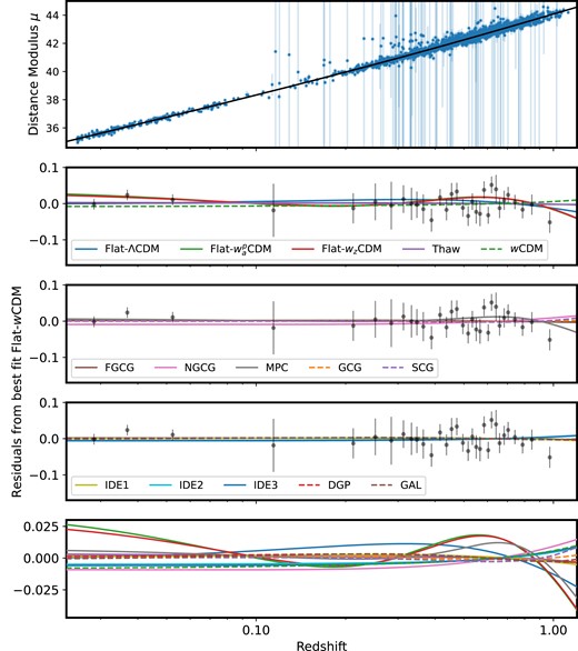
Upper panel: Hubble diagram of DES-SN5YR with the overlaid best-fitting Flat-wCDM model. We also show the inflated distance uncertainties from likely contaminants. Four lower panels: The difference between the data and the best-fitting Flat-wCDM model from the DES-SN5YR alone. We also overplot the best fit for each model (we exclude the Timescape model as it was fit against a modified Hubble diagram). Spatially flat models are shown as solid lines and models that allow curvature are represented by dashed lines.
Results for the cosmological models investigated in this work. These are the medians of the marginalized posterior with 68.27 per cent integrated uncertainties (‘cumulative’ option in ChainConsumer).
| Key paper results | |$\Omega _{\mathrm{m}}$| | |$\Omega _{\Lambda }$| | |$w_0$| | |$w_{a}$| | ||
|---|---|---|---|---|---|---|
| DES-SN5YR | ||||||
| Flat-|$\Lambda$|CDM | |$0.352\pm 0.017$| | – | – | – | – | – |
| |$\Lambda$|CDM | |$0.291^{+0.063}_{-0.065}$| | |$0.55\pm 0.10$| | – | – | – | – |
| Flat-wCDM | |$0.264^{+0.074}_{-0.096}$| | – | |$-0.80^{+0.14}_{-0.16}$| | – | – | – |
| Flat-|$w_0 w_a$|CDM | |$0.495^{+0.033}_{-0.043}$| | – | |$-0.36^{+0.36}_{-0.30}$| | |$-8.8^{+3.7}_{-4.5}$| | – | – |
| Cosmography | |$q_0$| | |$j_0$| | |$s_0$| | |||
| DES-SN5YR | ||||||
| Third order | |$-0.362^{+0.067}_{-0.069}$| | |$0.16^{+0.32}_{-0.29}$| | – | |||
| Fourth order | |$-0.06^{+0.11}_{-0.13}$| | |$-2.43^{+0.92}_{-0.72}$| | |$1.4^{+4.6}_{-3.3}$| | |||
| Parametric models | |$\Omega _{\mathrm{m}}$| | |$\Omega _{\rm de}$| | |$w_0$| | |$w_{z}$| | |$w^p_0$| | |$w_{a}$| |
| DES-SN5YR | ||||||
| wCDM | |$0.262^{+0.068}_{-0.074}$| | |$0.61^{+0.26}_{-0.25}$| | |$-0.91^{+0.20}_{-0.43}$| | – | – | – |
| Flat-|$w_0 w_z$|CDM | |$0.492^{+0.027}_{-0.038}$| | – | |$-0.57\pm 0.23$| | |$-6.0^{+2.5}_{-2.4}$| | – | – |
| Flat-|$w^{\rm p}_0 w_a$|CDM where |$z_p$| = |$0.078$| | |$0.495^{+0.034}_{-0.045}$| | – | – | – | |$-1.00^{+0.13}_{-0.14}$| | |$-8.6^{+3.8}_{-4.5}$| |
| DES-SN5YR + CMB-R + BAO-|$\theta _*$| | ||||||
| wCDM|$^{\dagger }$| | |$0.320\pm 0.007$| | |$0.682\pm 0.007$| | |$-0.912\pm 0.029$| | – | – | – |
| Flat-|$w_0 w_z$|CDM|$^{\dagger }$| | |$0.322\pm 0.007$| | – | |$-0.866^{+0.046}_{-0.042}$| | |$-0.142^{+0.093}_{-0.123}$| | – | – |
| Flat-|$w^{\rm p}_0 w_a$|CDM|$^{\dagger }$| where |$z_p$| = |$0.274$| | |$0.323\pm 0.007$| | – | – | – | |$-0.918\pm 0.027$| | |$-0.29^{+0.26}_{-0.28}$| |
| Thawing scaling field model | |$\Omega _{\mathrm{m}}$| | |$w_0$| | |$\alpha$| | – | – | – |
| DES-SN5YR | ||||||
| Thaw | |$0.306^{+0.041}_{-0.042}$| | |$-0.83^{+0.12}_{-0.14}$| | |$1.452^{+0.067}_{-0.068}$| | – | – | – |
| DES-SN5YR + CMB-R + BAO-|$\theta _*$| | ||||||
| Thaw | |$0.323\pm 0.007$| | |$-0.867^{+0.041}_{-0.040}$| | |$1.449^{+0.072}_{-0.065}$| | – | – | – |
| Chaplygin gas | |$\Omega _{\mathrm{m}}$| | A | |$\zeta$| | |$w_0$| | ||
| DES-SN5YR | ||||||
| SCG|$^{*}$| | |$0.121\pm 0.035$| | |$0.789^{+0.029}_{-0.027}$| | – | – | – | – |
| FGCG | |$0.255^{+0.099}_{-0.133}$| | |$0.600^{+0.049}_{-0.048}$| | |$-0.33^{+0.33}_{-0.30}$| | – | – | – |
| GCG | |$0.236^{+0.080}_{-0.124}$| | |$0.65^{+0.15}_{-0.12}$| | |$-0.01^{+1.09}_{-0.73}$| | – | – | – |
| NGCG | |$0.278^{+0.095}_{-0.147}$| | |$0.76^{+0.15}_{-0.27}$| | |$0.03^{+1.15}_{-0.66}$| | |$-0.78^{+0.16}_{-0.45}$| | ||
| DES-SN5YR + CMB-R + BAO-|$\theta _*$| | ||||||
| SCG|$^{*}$| | |$0.376\pm 0.009$| | |$0.556\pm 0.008$| | – | – | – | – |
| FGCG|$^{\dagger }$| | |$0.322\pm 0.007$| | |$0.636^{+0.020}_{-0.019}$| | |$-0.107^{+0.038}_{-0.035}$| | – | – | – |
| GCG|$^{\dagger }$| | |$0.319\pm 0.008$| | |$0.634^{+0.021}_{-0.022}$| | |$-0.120^{+0.042}_{-0.041}$| | – | – | – |
| NGCG | |$0.323\pm 0.007$| | |$0.777^{+0.087}_{-0.125}$| | |$0.33^{+0.44}_{-0.40}$| | |$-0.77^{+0.11}_{-0.20}$| | – | – |
| Cardassian | |$\Omega _{\mathrm{m}}$| | q | n | – | – | – |
| DES-SN5YR | ||||||
| MPC|$^{\dagger }$| | |$0.467^{+0.032}_{-0.054}$| | |$13.3^{+4.7}_{-6.5}$| | |$0.464^{+0.034}_{-0.040}$| | – | – | – |
| DES-SN5YR + CMB-R + BAO-|$\theta _*$| | ||||||
| MPC | |$0.322^{+0.007}_{-0.006}$| | |$1.38^{+0.49}_{-0.42}$| | |$0.25^{+0.12}_{-0.20}$| | – | – | – |
| Interacting Dark Energy | |$\Omega _{\mathrm{m}}$| | |$w_0$| | |$\varepsilon$| | – | – | – |
| DES-SN5YR | ||||||
| IDE1 | |$0.54^{+0.19}_{-0.32}$| | |$-1.30^{+0.53}_{-0.91}$| | |$0.46^{+0.90}_{-0.53}$| | – | – | – |
| IDE2 | |$0.31^{+0.22}_{-0.14}$| | |$-0.85^{+0.17}_{-0.43}$| | |$0.10^{+0.24}_{-0.36}$| | – | – | – |
| IDE3 | |$0.28^{+0.30}_{-0.21}$| | |$-0.82^{+0.21}_{-0.60}$| | |$0.12^{+0.86}_{-1.12}$| | – | – | – |
| DES-SN5YR + CMB-R + BAO-|$\theta _*$| | ||||||
| IDE1 | |$0.53^{+0.18}_{-0.30}$| | |$-1.38^{+0.55}_{-0.91}$| | |$0.47^{+0.89}_{-0.54}$| | – | – | – |
| IDE2|$^{\dagger }$| | |$0.323\pm 0.007$| | |$-0.919\pm 0.032$| | |$0.000\pm 0.001$| | – | – | – |
| IDE3 | |$0.25^{+0.15}_{-0.10}$| | |$-0.80^{+0.13}_{-0.26}$| | |$-0.18^{+0.37}_{-0.28}$| | – | – | – |
| Modified gravity | |$\Omega _{\mathrm{m}}$| | |$\Omega _{\mathrm{k}}$| | |$\Omega _{\mathrm{rc}}$| | |$\Omega _{\mathrm{g}}$| | – | – |
| DES-SN5YR | ||||||
| DGP|$^{*}$| | |$0.231^{+0.047}_{-0.051}$| | |$0.03^{+0.18}_{-0.17}$| | |$0.141^{+0.024}_{-0.025}$| | – | – | – |
| GAL|$^{*}$| | |$0.298^{+0.074}_{-0.073}$| | |$0.34\pm 0.15$| | – | |$0.362^{+0.082}_{-0.078}$| | – | – |
| DES-SN5YR + CMB-R + BAO-|$\theta _*$| | ||||||
| DGP|$^{*}$| | |$0.342\pm 0.009$| | |$0.014\pm 0.003$| | |$0.105\pm 0.003$| | – | – | – |
| GAL|$^{*}$| | |$0.292\pm 0.007$| | |$-0.013\pm 0.004$| | – | |$0.720\pm 0.007$| | – | – |
| Timescape | |$\Omega _{\mathrm{m}}^{\S}$| | |$f_{v0}$| | – | – | – | – |
| DES-SN5YR|$_{\mathrm{cut}}$| | ||||||
| Timescape|$^{*}$| | |$0.292^{+0.043}_{-0.051}$| | |$0.791^{+0.039}_{-0.034}$| | – | – | – | – |
| Flat-|$\Lambda$|CDM | |$0.362^{+0.019}_{-0.018}$| | – | – | – | – | – |
| DES-SN5YR|$_{\mathrm{cut}}$| + BAO-|$\theta _{*\perp }$| | ||||||
| Timescape|$^{*}$| | |$0.446^{+0.010}_{-0.009}$| | |$0.665^{+0.008}_{-0.009}$| | – | – | – | – |
| Flat-|$\Lambda$|CDM | |$0.332^{+0.011}_{-0.010}$| | – | – | – | – | – |
Notes.|$^{*}$| Cannot reduce to the cosmological constant for any set of parameters.
|$^{\dagger }$| Best fits are |$\gt 2\sigma$| from the subset of parameters that reduce to the cosmological constant.
|$^{\S}$| We convert the constraint on the void fraction to the dressed matter density, which is related by |$\Omega _{\mathrm{m} }=\frac{1}{2}\left(1-f_{\mathrm{v} 0}\right)\left(2+f_{\mathrm{v} 0}\right)$|.
7.1 Cosmography
The cosmographic approach is a smooth Taylor expansion of the scale factor, a that makes minimal assumptions about the underlying cosmological model, however retains the assumptions of homogeneity and isotropy (Visser 2004; Zhang, Li & Xia 2017; Macaulay et al. 2019). In cosmography, its useful to define the deceleration parameter,
the jerk parameter,
and the snap parameter,
where q is directly related to the accelerated expansion of the universe and |$j=1$| at all times for a spatially flat universe with a cosmological constant. Here, we Taylor expand the scale factor for a flat universe and take the series expansion to four terms,
where |$\mathcal {C}_{1} = \left(1+q_0\right)$|, |$\mathcal {C}_{2} = \frac{1}{2} \left(j_0-q_0^2\right)$|, |$\mathcal {C}_{3} = \frac{1}{6} \left(3q_0^{2} + 3q_0^3-4q_0 j_0-3 j_0-s_0\right)$|, and |$q_0$|, |$j_0$|, and |$s_0$| are the current epoch deceleration, jerk, and snap parameters, respectively.
We fit cosmographic expansion to third [equation (22) excluding the |$z^3$| term] and fourth order (equation 22) with our constraints shown in Fig. 10. For the third order fit we find |$q_0=-0.362^{+0.067}_{-0.069}$| and evidence for an accelerating universe at |$\gt 5\sigma$|. When we fit to fourth order, we find |$q_0=-0.06^{+0.11}_{-0.13}$|, which is consistent with zero however we note that the snap parameter is poorly constrained by the DES-SN5YR alone and find |$s_0=1.4^{+4.6}_{-3.3}$|. This result is analogous to the DES-SN5YR key paper results on the Flat-|$w_0 w_a$|CDM model who find a |$w_0$| consistent with zero when |$w_a$| is included in the fit. We also ensured that our fits were not over influenced by a particular redshift range and found consistent results after (a) removing low-z data using the DES SNe alone and (b) removing high-z SNe at |$z\gt 0.80$|.
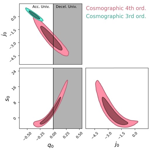
Constraints for the |$3^{\rm rd}$| and |$4^{\rm th}$| order cosmographic models (Section 7.1) from the DES-SN5YR data set only. The contours represent the 68.3 and 95.5 per cent confidence intervals.
7.2 Parametric models for the equation of state
The parametric models we consider here consider time varying dark energy with different functional forms of the dark energy equation of state, w. When all components have a constant equation of state, Friedmann’s equation is simply
where the sum is over matter (|$w_m=0$|), curvature (|$w_k=-1/3$|), and dark energy with a constant equation of state (|$w_{\rm de}={\rm constant}$|), which could be a cosmological constant (|$w_\Lambda =-1$|). Radiation (|$w_r=1/3$|) could also be included but is negligible for our redshift range. When testing dark energy with a time-varying equation of state one needs to make the substitution,
The simplest parametric model is where w is generalized to an arbitrary constant while retaining spatial flatness (Flat-wCDM). This is the baseline cosmological model used within the DES-SN5YR analysis (DES Collaboration 2024b), who also test a flat model with a time varying dark energy in the form of |$w(a)=w_0+w_a(1-a)$| (Flat-|$w_0 w_a$|CDM). While we do not refit these models here, we convert the constraints on Flat-|$w_0 w_a$|CDM using a linear variation of |$w(a)$|, which is anchored to a pivot redshift |$z_p$| instead of |$z=0$| (Flat-|$w^{\rm p}_0 w_a$|CDM), such that |$w^{\rm p}(a)=w^{\rm p}_0+w^{\rm p}_a(a_{\rm p}-a)$|, where |$w_0^{\rm p}=w_0+w_a(1-a_{\rm p})$|, |$w_a^{\rm p}=w_a$|, and |$a_{\rm p}=1/(1+z_{\rm p})$|. The pivot redshift corresponds to the redshift resulting in the tightest constraints on |$w(a)$| (Huterer & Turner 2001). The expansion rate for the Flat-|$w^{\rm p}_0 w_a$|CDM model is given by
and in the case |$z_p=0$|, |$a_{\rm p}=1$| the Flat-|$w_0 w_a$|CDM parametrization is recovered.
We also test two other parametrizations. First, the DES-SN5YR baseline model with spatial curvature as an additional free parameter (wCDM). Secondly, a model where |$w(a)$| varies linearly in redshift instead of scale factor (Flat-|$w_0 w_z$|CDM), such that |$w(z) = w_0 + w_z z$| (Weller & Albrecht 2002) and results in a Friedmann equation given by
Results for the parametric forms of the equation of state that we test within this work are summarized in Table 5 and the associated contours are plotted in Fig. 11.
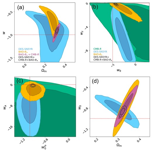
Parametric models, (a) wCDM, (b) Flat-|$w_0 w_z$|CDM, (c) Flat-|$w^{\rm p}_0 w_a$|CDM (see Section 7.2) and the (d) thawing model (Section 7.3): Constraints from the DES-SN5YR data set only (blue), a prior from the CMB-R (green), BAO-|$\theta _*$| (orange), CMB-R + BAO-|$\theta _*$| (purple) as well as the DES-SN5YR combined with both the CMB-R and BAO-|$\theta _*$| priors (overlaid black contours). The contours represent the 68.3 and 95.5 per cent confidence intervals. The red dashed lines mark the parameters that recover a cosmological constant.
Using the DES-SN5YR alone, the wCDM model is statistically consistent with a cosmological constant value of |$w=-1$|; however both Flat-|$w_{z}$|CDM and Flat-|$w^{\rm p }_{a}$|CDM favour a time-varying component to w that increases with time. We note that the Flat-|$w_0w_a$|CDM model was constrained in DES Collaboration (2024b) finding |$(w_0, w_a)=(-0.36^{+0.36}_{-0.30}, -8.8^{+3.7}_{-4.5}$|) using DES-SN5YR alone. Here, we refit and convert these results to the equation of state at the pivot redshift and find |$(w^{p}_0, w_a, z_p) = (-1.00^{+0.13}_{-0.14}, -8.6^{+3.8}_{-4.5}, 0.078)$|.
When we combine DES-SN5YR with the CMB-R and BAO-|$\theta _*$| our results are still consistent with a time-varying component to w that increases with time with the best fit |$w_{z}$| and |$w_a$| (we find |$z_p=0.274$| for the pivot redshift) both remaining |$\gt 1\sigma$| from a static w.
Interestingly, with the combined data sets, all parametric forms of the dark energy equation of state result in a best fit |$w\gt 1\sigma$| from a cosmological constant and all favour a |$w\gt -1$|.
7.3 ‘Thawing’ scalar field models
Light scalar fields provide a dynamical model for evolving dark energy inspired by scalar field models for primordial inflation. In the simplest incarnation of these models, the true vacuum energy density (or cosmological constant) of the universe is assumed to be zero, and dark energy is a transient phenomenon arising from the fact that a classically evolving scalar field |$\phi$| with effective mass |$m_\phi \lesssim H_0$| has not yet have reached its ground state. In most particle physics models, light scalars are not technically natural, so it is conventional to consider models in which the small scalar mass is protected by a weakly broken shift symmetry, as is the case for the pseudo-Nambu-Goldstone boson (PNGB) model introduced by Frieman et al. (1995).
Assuming the canonical Lagrangian for a scalar field, |${\cal {L}}= (1/2)g^{\mu \nu }\partial _\mu \phi \partial _\nu \phi -V(\phi)$|, neglecting spatial perturbations the equation of motion of the field in an expanding universe is given by
where the expansion rate is given by
|$M_{Pl}=G^{-1/2}$| is the Planck mass, and the energy density of the field is
The time-evolution of |$\rho _\phi$| is determined by H and by the equation-of-state parameter, |$w_\phi =p_\phi /\rho _\phi$|, where the scalar field pressure is
For a given form of the potential |$V(\phi)$| and initial value of the scalar field, |$\phi (t_i) \equiv \phi _i$| at some early time |$t_i \ll t_0$|, this dynamical system can be solved to obtain |$\phi (t)$| and thus the expansion history (assuming spatial flatness)
where |$\rho _{\rm crit}=3M_{Pl}^2H_0^2/8\pi$|.
For ‘thawing’ scalar field models [the thawing/freezing nomenclature is from Caldwell & Linder (2005)], which include standard potentials of the form |$V=(1/2)m_\phi ^2 \phi ^2 + \lambda \phi ^4$| (with |$\lambda \gt 0$|), the PNGB model |$V(\phi)=m^2 f^2(1-\cos (\phi /f))$|, and polynomials |$V(\phi)=\sum _{i=1}^{n}a_i\phi ^i$| with |$a_i \ge 0$|, at early times the driving term |${\rm d}V/{\rm d}\phi$| in equation (27) is subdominant compared to the Hubble-damping term |$3H\dot{\phi }$|. In this limit, the field is effectively frozen at its initial value |$\phi _i$|, hence |$\dot{\phi }(t_i)=0$|, |$\rho _\phi (t_i)=V(\phi _i)$|, and |$w_\phi (t_i)=-1$|. Once the expansion rate drops below the curvature of the potential, |$H \lesssim \sqrt{|{\rm d}^2V/{\rm d}\phi ^2|}$|, the field begins to roll down the potential, develops non-negligible kinetic energy, and |$w_\phi$| grows from |$-1$|. The parameters of |$V(\phi)$| and the value of |$\phi _i$| jointly determine |$w_\phi (t)$| and the current scalar energy density, |$\Omega _\phi =\rho _\phi (t_0)/\rho _{\rm crit}$|.
For example, for a free, massive scalar with |$V=(1/2)m_\phi ^2 \phi ^2$| the condition |$\Omega _m=0.3$| implies |$(m_\phi /H_0)(\phi (t_0)/M_{Pl}) \simeq 0.4$| in the limit where |$\dot{\phi }^2 \ll V(\phi)$|. For |$m_\phi /H_0 \gtrsim 1$||$(\lesssim 1)$| the field begins rolling before the present epoch (or not) and the present value of the equation-of-state parameter, |$w_0 \equiv w_\phi (t_0)$|, can be measurably above |$-1$| (or not), |$w_0 \simeq -1+(1/7)(m_\phi /H_0)^2$|.
While there have been a variety of approximate solutions and fits to late-time scalar field evolution (e.g. Dutta & Scherrer 2008; de Putter & Linder 2008; Chiba 2009), numerical experiments show that the redshift-evolution of |$w_\phi$| for thawing models is very well approximated by
where the value of |$\alpha$| is only very weakly dependent on |$w_0$| and on the form of |$V(\phi)$| and is generally in the narrow range |$\alpha =1.35-1.55$|. As a consequence, these models are characterized by a quasi-1D parameter space that can be taken to be |$w_0$| (with |$\alpha =1.45\pm 0.1$|). This approximation holds if the effective scalar mass |$m_\phi$| is not large compared to |$H_0$| (otherwise, the field will begin oscillating around the minimum of its potential by the present epoch.)
In Fig. 11, we show constraints on |$w_0$| and |$\Omega _m$| marginalized over the narrow thawing-model prior on |$\alpha$|. For DES-SN5YR alone, we find |$\Omega _m=0.306^{+0.041}_{-0.042}$| and |$w_0=-0.83^{+0.12}_{-0.14}$|; including CMB and BAO measurements, the resulting constraints are |$\Omega _m=0.323\pm 0.007$| and |$w_0=-0.867^{+0.041}_{-0.040}$|, i.e. a |$3\sigma$| deviation from |$w_0=-1$|. As shown in Table 6, for the combined data sets the thawing model is moderately preferred over |$\Lambda$|CDM based on the AIC.
Goodness of fit and model comparison statistics. A more negative |$\frac{1}{2}\Delta$|AIC and |$\Delta {\rm ln}~S$| value indicates a stronger preference over Flat-|$\Lambda$|CDM.
| DES-SN5YR | DES-SN5YR + CMB-R + BAO-|$\theta _*$| | ||||||
|---|---|---|---|---|---|---|---|
| Model | |$\frac{1}{2}\Delta$|AIC | |$\Delta {\rm ln}~S$| | |$\chi ^2$| | Model | |$\frac{1}{2}\Delta$|AIC | |$\Delta {\rm ln}~S$| | |$\chi ^2$| |
| Cosmography – Third Order | |$-0.9$| | |$-1.37$| | 1641 | – | – | – | – |
| Cosmography – Fourth Order | |$-3.6$| | |$-4.39$| | 1633 | – | – | – | – |
| Flat-|$\Lambda$|CDM | 0.0 | 0.0 | 1645 | Flat-|$\Lambda$|CDM | 0.0 | 0.0 | 1665 |
| |$\Lambda$|CDM | 0.6 | 0.09 | 1644 | |$\Lambda$|CDM | 0.4 | |$-0.10$| | 1664 |
| wCDM | 1.1 | 0.13 | 1643 | wCDM | |$-3.1$| | |$-3.64$| | 1655 |
| Flat-|$w_0 w_z$|CDM | |$-1.8$| | |$-2.97$| | 1637 | Flat-|$w_0 w_z$|CDM | |$-3.1$| | |$-4.16$| | 1655 |
| Flat-|$w^{p}_{a}$|CDM | |$-1.8$| | |$-2.58$| | 1637 | Flat-|$w^{p}_{a}$|CDM | |$-3.2$| | |$-4.17$| | 1655 |
| Thaw | 1.0 | |$-0.57$| | 1643 | Thaw | |$-3.2$| | |$-4.60$| | 1655 |
| SCG | 0.9 | 0.35 | 1644 | SCG | 138.4 | 138.03 | 1940 |
| FGCG | 0.4 | |$-0.30$| | 1643 | FGCG | |$-3.4$| | |$-3.94$| | 1657 |
| GCG | 0.4 | 0.08 | 1641 | GCG | |$-2.7$| | |$-3.71$| | 1656 |
| NGCG | 0.6 | 0.03 | 1642 | NGCG | |$-3.2$| | |$-4.08$| | 1655 |
| MPC | |$-1.8$| | |$-2.49$| | 1637 | MPC | |$-3.2$| | |$-3.94$| | 1655 |
| IDE1 | 1.3 | |$-0.17$| | 1643 | IDE1 | |$-2.7$| | |$-3.70$| | 1656 |
| IDE2 | 0.7 | |$-0.23$| | 1642 | IDE2 | |$-2.7$| | |$-3.75$| | 1656 |
| IDE3 | 0.1 | |$-0.26$| | 1641 | IDE3 | |$-3.2$| | |$-3.82$| | 1655 |
| DGP | 0.6 | |$-0.05$| | 1644 | DGP | 31.5 | 31.11 | 1726 |
| GAL | 0.9 | 0.34 | 1644 | GAL | 72.5 | 72.10 | 1808 |
| DES-SN5YR|$_{\mathrm{cut}}$| | DES-SN5YR|$_{\mathrm{cut}}$| + BAO-|$\theta _{*\perp }$| | ||||||
| Flat-|$\Lambda$|CDM | 0.0 | 0.0 | 1616 | Flat-|$\Lambda$|CDM | 0.0 | 0.0 | 1624 |
| Timescape | |$-1.7$| | |$-1.72$| | 1612 | Timescape | 6.3 | 6.17 | 1637 |
The current data provide no meaningful constraint on the parameter |$\alpha$| that determines the speed with which |$w_\phi$| grows from its asymptotic value of |$-1$|. That is, if we widen the theory prior on |$\alpha$| to allow values |$\alpha \gg 1$|, the best-fitting values are very large, with very large uncertainties. Note that for |$\alpha \gg 1$|, |$w(z)=-1$| down to very low redshift |$z \ll 1$|, so cosmic distances versus redshift should be indistinguishable from those in |$\Lambda$|CDM.
7.4 Chaplygin gas models
Chaplygin gas models deviate from |$\Lambda$|CDM by invoking an exotic background fluid with an equation of state |$p= -A \rho ^{-\zeta }$| (Kamenshchik, Moschella & Pasquier 2001; Bento, Bertolami & Sen 2002; Fabris, Gonçalves & Ribeiro 2004) where A is a positive constant. Chaplygin gas models represent pressure-less dark matter in the early universe and dark energy in recent times and therefore may also be able to unify dark matter and dark energy (Bilić, Tupper & Viollier 2002).
The simplest form of Chaplygin gas, which was introduced by Kamenshchik et al. (2001), has an equation of state |$p\propto \rho ^{-1}$| (|$\zeta = 1$|). This model is referred to as the Standard Chaplygin Gas (SCG) model with a Friedmann equation given by
SCG has been shown to be inconsistent with other data sets (Bean & Doré 2003; Sandvik et al. 2004; Davis et al. 2007) however will be re-tested within this work.
Generalized Chaplygin Gas (GCG), which maintains |$\zeta$| as a free parameter, results in a Friedmann equation given by
and reduces to |$\Lambda$|CDM for |$\zeta = 0$| and |$\Omega _m = (1-\Omega _k)(1-A)$|.
We note that as |$\Lambda$|CDM is recovered for |$\zeta = 0$|, the SCG model (which has |$\zeta =1$|) cannot reduce to |$\Lambda$|CDM for any parameter choice. As a result it may not be surprising that, in contrast to the SCG model, the GCG model has been shown to be consistent with the previous data combinations (Davis et al. 2007; Barreiro, Bertolami & Torres 2008; Sollerman et al. 2009; Xu & Lu 2010; Zhai et al. 2017) consisting of the ESSENCE, SDSS-II, Constitution, and Pantheon SN data sets (Sako et al. 2007; Wood-Vasey et al. 2007; Hicken et al. 2009; Scolnic et al. 2018).
Barreiro et al. (2008) suggest that GCG can be thought of as an interacting form of |$\Lambda$|CDM. The analogous interacting form of wCDM was proposed by Zhang, Wu & Zhang (2006) termed New Generalized Chaplygin Gas (NGCG). The Friedmann equation for the spatially flat NGCG model is given by
and can be reduced to wCDM for |$\zeta = 0$|.
In Fig. 12 we present the contours for the Chaplygin gas models we investigate in this work. Constrained by the DES-SN5YR alone, the SCG model provides the lowest central value for the matter density of all models tested within this work at |$\Omega _{\rm m}=0.121\pm 0.035$|. We note that this is due to the model favouring a high curvature, equivalent to |$\Omega _{\rm k}=0.43\pm 0.12$|. When combined with external priors, the SCG model is unable to simultaneously fit the different data sets (see Fig. 12a), which show extremely strong disagreement in the best-fitting parameters and highlighted by the poor Akaike Information Criterion (AIC) result of |$\Delta$|AIC|$=276.9$| relative to Flat-|$\Lambda$|CDM (see Section 8.2 and Table 6).
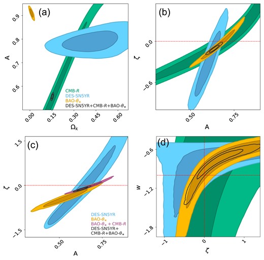
Chaplygin Gas models, (a) SCG, (b) FGCG, (c) GCG, and (d) NGCG (Section 7.4): Constraints from the DES-SN5YR data set only (blue), a prior from the CMB-R (green), BAO-|$\theta _*$| (orange), CMB-R + BAO-|$\theta _*$| (purple) as well as the DES-SN5YR combined with both the CMB-R and BAO-|$\theta _*$| priors (overlaid black contours). The contours represent the 68.3 and 95.5 per cent confidence intervals. The red dashed lines mark the parameters that recover a cosmological constant.
Using the DES-SN5YR alone, the remaining Chaplygin Gas models FGCG, GCG and NGCG are consistent within |$1\sigma$| (|$\zeta =0$| and |$w=-1$| for NGCG) of a cosmological constant. When combined with the CMB-R and BAO-|$\theta _*$| both the FGCG and GCG models find |$\zeta \gt 1\sigma$| from a cosmological constant. For the NGCG model, the best fit |$\zeta$| is consistent with a cosmological constant, however favouring |$w\gt -1$|.
7.5 Cardassian models
Cardassian models, first proposed by Freese & Lewis (2002), deviate from |$\Lambda$|CDM with the following modification to the Friedmann–Lemaítre–Robertson–Walker metric (FLRW) equation,
where the usual FLRW equation is recovered for |$B=0$|. Cardassian models invoke no vacuum energy (|$\Lambda = 0$|), instead the additional term in equation (36) (|$B\rho ^n$|) is initially negligible and only begins to dominate in recent times. Once the second term dominates, it causes the universe to accelerate. Therefore, with this modification, pure matter (or radiation) alone can drive an accelerated expansion. Some motivations for the addition of this term have been suggested and include self-interaction of dark matter (Gondolo & Freese 2002), as well as the embedding of our observable 3D brane in a higher dimensional universe (Chung & Freese 2000). The original power-law Cardassian model results in a Friedmann equation of the same functional form as that of wCDM where |$w = n-1$| and therefore does not need to be tested separately. Wang et al. (2003) generalizes this model by introducing an additional free parameter |$q \gt 0$|. This model is called Modified Polytropic Cardassian (MPC) expansion which follows,
and collapses to Flat-w CDM for |$q=1$| where |$w = n-1$|.
Our constraints in the |$n-q$| plane for MPC expansion are shown in Fig. 13(a). We find |$q=13.3^{+4.7}_{-6.5}$| using DES-SN5YR alone, inconsistent with |$q=1$| by |$\sim 2\sigma$|. This result is inconsistent with previous analyses by Zhai et al. (2017) and Magañ aet al. (2018) however these analyses both include constraints from probes other than SN. Our results are consistent with these previous analyses and |$q=1$| when we supplement the DES-SN5YR data with external probes, we find |$q=1.38^{+0.49}_{-0.42}$|.

7.6 Interacting dark energy and dark matter
In typical cosmological models, dark matter and dark energy are assumed to evolve independently. However, dark energy and dark matter provide the largest contribution to the energy budget of the universe so it is worth investigating if these components can interact. Interacting dark energy and dark matter (IDE) models are therefore those which allow for this interaction (Freese et al. 1987) and are desirable as they allow solutions with a constant dark energy to matter ratio, solving the coincidence problem.
In this paper, we consider a popular subset (Barnes et al. 2005; Guo, Ohta & Tsujikawa 2007; Li et al. 2009; He et al. 2010; Li & Zhang 2014; Hu et al. 2016; Wang et al. 2016; von Marttens et al. 2019) of IDE models where the total energy density of dark energy and dark matter is conserved, however, the particular densities evolve as,
where |${\rho }_{\rm m}$| and |${\rho }_{x}$| represent the density of matter and dark energy, respectively, w is the dark energy equation of state, and Q is the interaction kernel which indicates the rate of energy transfer between the two components.
We investigate three spatially flat IDE models where Q has the general form |$Q = H\varepsilon f(\rho _x, \rho _{\rm m})$|, the function |$f(\rho _x, \rho _{\rm m})$| specifies a particular IDE model, and |$\varepsilon$| is the coupling parameter between the dark components. The sign of |$\varepsilon$| describes the energy flow between the interacting components where |$\varepsilon \lt 0$| corresponds to a flow of energy from dark matter to dark energy. The parametrizations of Q and the respective Friedmann equations are:
- IDE1: |$Q = 3H\varepsilon \rho _{x}$|(39)$$\begin{eqnarray} E(z)^2=\Omega _{\mathrm{m}}a^{-3} +\Omega _{x}\biggr [\frac{\varepsilon ~ a^{-3}}{w + \varepsilon } + \frac{w~ a^{-3\left(1+w+\varepsilon \right)}}{w + \varepsilon }\biggr ] \end{eqnarray}$$
- IDE2: |$Q = 3H\varepsilon \rho _{\rm m}$|(40)$$\begin{eqnarray} E(z)^2=\frac{\Omega _{x}}{a^{3\left(1+w\right)}} {{\displaystyle +}} \Omega _{\mathrm{m}}{{\displaystyle \biggr [{ \frac{\varepsilon ~a^{-3\left(1+w\right)}}{w + \varepsilon }{{\displaystyle +}}\frac{w~a^{-3\left(1-\varepsilon \right)}}{w + \varepsilon }} \biggr ]}} \end{eqnarray}$$
IDE3: |$Q = 3H \varepsilon \frac{\rho _{\rm m} \rho _x}{\rho _{\rm m} + \rho _x}$|
where
The IDE models in equations (39), (40), and (41) will be referred to, respectively, as IDE1, IDE2, and IDE3 throughout this work. The results for the three IDE models we test are summarized in Table 5 and the contours are shown in Fig. 13.
Using DES-SN5YR alone and after combining the DES-SN5YR with priors from the CMB-R and BAO-|$\theta _*$| all of the IDE models tested are consistent within |$1\sigma$| of no interaction between the dark components, |$\varepsilon =0$| and |$w=-1$|.
We also note that the CMB-R puts a stringent constraint on the interaction for the IDE2 model, where we find |$\varepsilon = 0.000\pm 0.001$|. The tightness of the constraint on |$\varepsilon$| is expected and in agreement with previous works (Guo et al. 2007; Wang et al. 2016). This is due to the CMB-R data not allowing a large deviation from the standard matter-dominated epoch along with the second term in equation (40).
7.7 Modified gravity
Dvali-Gabadadze-Porrati (DGP) brane world models first introduced by Dvali, Gabadadze & Porrati (2000) arise from a mechanism where the observed 4D gravity is embedded on a brane in 5D Minkowski space. As a result, locally the gravitational potential propagates in four dimensions reducing to General Relativity. However, at large distances the gravitational potential propagates in 5D or ‘leaks out into the bulk’ deviating from General Relativity and causing accelerated expansion. Two branches of cosmological solutions in the DGP model have distinct properties. The solution examined in this work is the so-called self-accelerating branch where the late-time acceleration of the universe occurs without the need of a cosmological constant (Deffayet 2001) and is described by
where |$\Omega _{m} =1-\Omega _k-2 \sqrt{\Omega _{r_{c}}} \sqrt{1-\Omega _k}$| and the length scale for which the ‘leaking’ takes place is |$r_{c}$| and |$\Omega _{r_{c}} = 1/4 r^2_{c} H_{0}^{2}$|. Therefore, the Flat-DGP and DGP models have the same number of free parameters as Flat-|$\Lambda$|CDM and |$\Lambda$|CDM, respectively.
Inspired by the DGP model, Deffayet, Deser & Esposito-Farèse (2009) and Nicolis, Rattazzi & Trincherini (2009) introduced Galileon cosmology, which is a scalar field class of models that are invariant under a shift symmetry in field space. Importantly, the Galileon scalar has no effect on the expansion rate during early times due to a natural screening mechanism, the Vainshtein effect in which non-linear effects can effectively decouple the scalar field from gravity (De Felice & Tsujikawa 2011). In late times, there exists a tracker solution (GAL) that is stable and self-accelerating with a very negative equation of state |$w\lt -1$|. The Friedmann equation for the GAL model has the same number of free parameters as |$\Lambda$|CDM and is given by
where |$\Omega _{g}=1-\Omega _m-\Omega _k$|. Both the DGP and GAL models provide a good fit to DES-SN5YR alone. However, when we include external probes, our results (summarized in Table 5) are in agreement with previous works (Lombriser et al. 2009; Li et al. 2011; Xu & Zhang 2016; Zhai et al. 2017; Peirone et al. 2018) that show the DGP and GAL models to be inconsistent with multiple data sets, as seen in Figs 13(e) and (f).
7.8 Timescape cosmology
So far, the models examined all seek to explain the observed acceleration of the universe, assuming a FLRW geometry which is exactly homogeneous and isotropic. However, the local Universe is far from homogeneous and possesses a cosmic web of structures dominated in volume by voids. Timescape cosmology (Wiltshire 2007a, b, 2009) discards the approximation of a FLRW universe and instead considers a Buchert average (Buchert 2000) over spatially flat wall regions and negatively curved voids. While the Buchert formalism has been investigated in other works, Timescape cosmology also accounts for a geometry difference between the Buchert average and an observer in a gravitationally bound system within the wall regions, for a universe dominated by voids. Wiltshire (2008) shows that this two-scale model results in a difference in clock rates that accumulates over cosmic time. In this work we use the Timescape tracker solution where the luminosity distance is calculated as,
where
t is defined implicitly in terms of the redshift by
and
Note that |$f_{\mathrm{v} 0}$| is the current epoch void fraction and the only free parameter of the Timescape model (as we treat |$H_0$| as a nuisance parameter in this work), which is related to the |${\it dressed}$|13 matter density parameter by
The time, t and Hubble parameter, |$\bar{H}_0$| in equations (44), (45), (46), and (47) are the volume averaged values, which are related to values we observe in a wall region by
and
We note that an average expansion law only holds on scales greater than the statistical homogeneity scale, which corresponds to a CMB rest-frame redshift of the order of |$z \sim 0.021-0.040$| (Scrimgeour et al. 2012; Ntelis et al. 2017). In this work we adopt the value used to quote the key results in Dam et al. (2017) of |$z_{\mathrm{min}} = 0.033$|. We re-run the entire pipeline with this cut, which reduces our low-z sample by 68 SNe (see Section 6; from here on we will refer to this modified sample as DES-SN5YR|$_{\mathrm{cut}}$|). We also use CMB rest-frame redshifts excluding peculiar velocity corrections of the host galaxy, which are calculated assuming a standard FLRW model to remain consistent with previous work by Dam et al. (2017).
Finally, we retest the Flat-|$\Lambda$|CDM model with these same changes to make a consistent comparison between the two models. In addition to the above changes to the DES-SN5YR data, we also note that the conversion of redshift increments to a radial comoving distance involves different assumptions about spatial curvature in the FLRW and Timescape models [see Appendix D2 from Dam et al. (2017) for more details]. Therefore, we do not include the CMB-R summary statistic as outlined in Section 6.2.1 when constraining the Timescape and Flat-|$\Lambda$|CDM models and include only angular measurements on the BAO scale (BAO-|$\theta _{*\perp }$| from here on) from the SDSS data [|$D_M(z_*)/D_M(z)$| constraints from Table 4].
Using DES-SN5YR alone, we find |$f_{v0}=0.791^{+0.039}_{-0.034}$|, equivalent to a dressed matter density of |$\Omega _{\mathrm{m}} = 0.292^{+0.043}_{-0.051}$| and for Flat-|$\Lambda$|CDM find |$\Omega _{\mathrm{m}} = 0.362^{+0.019}_{-0.018}$|. These results are consistent with constraints found by Dam et al. (2017) using the JLA catalogue (Betoule et al. 2014). Fig. 14 shows consistent matter density predictions between Flat-|$\Lambda$|CDM in the baseline analysis and Flat-|$\Lambda$|CDM|$_{\mathrm{cut}}$| after including a redshift cut at |$z_{\rm min}=0.033$| and excluding peculiar velocity corrections. However both are just outside the 68 per cent confidence interval of the Planck TTTEEE-lowE prediction (|$\Omega _{\mathrm{m}} =0.3166\pm 0.0084$|; Aghanim et al. 2020). In contrast, the Timescape model has a lower central value for the matter density in agreement with Planck.
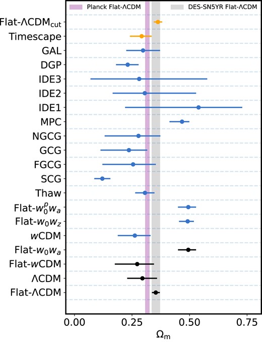
A summary of the best-fitting matter density for the models constrained by the DES-SN5YR sample. In black are the constraints from DES Collaboration (2024b), in blue and orange are constraints from this work, where the orange points highlight that the Hubble diagram used to constrain the Timescape and Flat |$\Lambda$|CDM|$_{\mathrm{cut}}$| models included a redshift cut at|$z_{\mathrm{min}}=0.033$| and excluded peculiar velocity corrections. The purple shaded region represents the TTTEEE-lowE 68 per cent confidence limits for the Flat-|$\Lambda$|CDM model determined by the Planck collaboration (Aghanim et al. 2020).
When combining the DES-SN5YR with BAO-|$\theta _{*\perp }$|, we find |$\Omega _{\mathrm{m}} = 0.446^{+0.010}_{-0.009}$| for the Timescape model and for Flat-|$\Lambda$|CDM find |$\Omega _{\mathrm{m}} = 0.332^{+0.011}_{-0.010}$|. These results are shown in Fig. 15. It is apparent from the upper panel that the data sets BAO-|$\theta _{*\perp }$| and DES-SN5YR are in tension in the Timescape model, and this model is therefore disfavoured relative to Flat-|$\Lambda$|CDM by the AIC statistic.
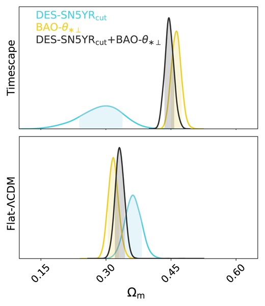
Constraints on the matter density from the DES-SN5YR|$_{\rm cut}$| data set only (blue) and BAO-|$\theta _{*\perp }$|(yellow) as well as the DES-SN5YR|$_{\rm cut}$| combined with BAO-|$\theta _{*\perp }$| prior (black). We show both the constraints from the Timescape and Flat-|$\Lambda$|CDM models (Section 7.8) with the same modifications to the data. In particular, we apply a redshift cut of|$z_{\mathrm{min}}=0.033$| and excluding peculiar velocity corrections. Note that for Timescape cosmology, the void fraction is related to the dressed matter density by |$\Omega _{\mathrm{m}}=\frac{1}{2}\left(1-f_{\mathrm{v} 0}\right)\left(2+f_{\mathrm{v} 0}\right)$|.
8 DISCUSSION
8.1 Goodness of fit
To investigate the goodness of fit for each of the models we present the |$\chi ^2$| for various data combinations, see Table 6, where |$\chi ^2=-2 \ln \mathcal {L}^{\max }$| and |$\mathcal {L}^{\rm max}$| is the maximum likelihood of the entire parameter space.
The number of degrees of freedom (|$N_{\rm dof}$|) is equal to the number of data points minus the number of cosmological parameters constrained for each model. For DES-SN5YR and DES-SN5YR|$_{\mathrm{cut}}$|, we approximate the number of data points by summing the BEAMS probability of each SN being Type Ia and find |$\sum P_{\mathrm{B}(\mathrm{Ia})}=1735$| and 1666, respectively. The additional number of data points when including the CMB-R, BAO-|$\theta _*$|, or BAO-|$\theta _{*\perp }$| are 1, 14, and 7, respectively.
Using DES-SN5YR alone, we find that all models tested within this work result in good fits to the data. However, the SCG, DGP, and GAL models have a poor |$\chi ^2$| when combining DES-SN5YR with the CMB-R and BAO-|$\theta _*$| as they are unable to reconcile the additional data sets. To a lesser extent this also afflicts the Timescape model. This can be seen visually in Figs 12(a), 13(e), 13(f), and 15 where the parameter space of the combined contours do not share a common region with all probes.
8.2 Model comparisons
To assess whether additional parameters invoked in the more complex models are justified given the data, we use the Akaike Information Criterion |${\rm AIC}\equiv 2k-2\ln \mathcal {L}^{\max }$| (Akaike 1974), where k is the number of parameters in the model. We also use the Suspiciousness (Handley & Lemos 2019), which is defined as |$\ln S= \ln R-\ln I$| where R is the Bayes Ratio and I is the Bayesian information. Handley & Lemos (2019) note that the Bayes ratio is prior-dependent and show that Suspiciousness is prior-independent due to the combination with the Bayesian information.
In Table 6 we quote the |$\frac{1}{2}\Delta$|AIC14 and the difference in the logarithm of the Suspiciousness, |$\Delta {\rm ln}~S$| relative to Flat-|$\Lambda$|CDM. To asses the strength of this preference, Trotta (2008) suggests that |$\Delta \gt 1$|, |$\Delta \gt 2.5$|, and |$\Delta \gt 5$| indicates weak, moderate, and strong evidence, respectively, against the model with the higher |$\Delta$| value. In both cases, more negative values indicate that the data prefers the extended model over Flat-|$\Lambda$|CDM. We determine ln|$~S$| using anesthetic software (Handley 2019) with the nested sampling outputs from polychord (Handley, Hobson & Lasenby 2015a, b) with |$25\times k$| live points, |$5\times k$| repeats, and an evidence tolerance requirement of 0.1.
Using the DES-SN5YR alone, both the AIC and Suspiciousness find no strong evidence for or against any of the non-standard models. Both find weak evidence for the third order cosmographic model and moderate evidence for the fourth order cosmographic model. Furthermore, the AIC and Suspiciousness weakly and moderately prefer the Flat-|$w_0 w_z$|CDM, Flat-|$w^{p}_{a}$|CDM, and MPC models over Flat-|$\Lambda$|CDM, respectively. The Timescape model, which was fit using the DES-SN5YR|$_{\rm cut}$| sample is weakly preferred by both the AIC and Suspiciousness.
When combined with the CMB-R and BAO-|$\theta _*$| both the AIC and Suspiciousness agree that 11 of the 15 non-standard models we investigate are moderately preferred over Flat-|$\Lambda$|CDM. We note that this is not a result of curvature alone with no preference for or against the |$\Lambda$|CDM model. The top performing models include Flat-|$w^{p}_{a}$|CDM with |$(\frac{1}{2}\Delta \mathrm{AIC}, \Delta {\rm ln}~S)=(-3.2, -4.17)$| indicating an evolution of w that increases with time, the thawing model with |$(\frac{1}{2}\Delta \mathrm{AIC}, \Delta {\rm ln}~S)=(-3.2, -4.60)$| and the FGCG model with |$(\frac{1}{2}\Delta \mathrm{AIC}, \Delta {\rm ln}~S)=(-3.4, -3.94)$|, which invokes an exotic background fluid. These results suggest that additional flexibility in our cosmological models may be required beyond the cosmological constant.
8.3 Tension metrics
We also use the Suspiciousness to assess whether different data sets are consistent (in contrast to Section 8.2 and Table 6 where the Suspiciousness was used as a model comparison statistic), which is ideal for cases such as ours where we have chosen deliberately wide and uninformative priors (See Lemos et al. 2021, Section 4.2). We use the anesthetic software (Handley & Lemos 2019) to determine ln|$~S$| and produce and ensemble of realizations to estimate sample variance. Using the scale from Trotta (2008), ln|$~S \lt -5$| is considered strong tension, |$-5 \lt $| ln|$~S \lt -2.5$| is considered moderate tension, and ln|$~S \gt -2.5$| indicates that the data sets are in agreement. In Fig. 16, we plot the |$\Delta$| ln |$~S$| between the relevant data sets. Note, models already been shown in Section 8.1 to be poor fits to the combined data sets (SCG, DGP, and GAL) have been excluded from the plot and all had |$\Delta$|ln|$~S \lt \lt -5$|. We find a strong tension between the DES-SN5YR with BAO-|$\theta _{*\perp }$| data sets when fitting the Timescape model. For all other models, we find no indication of tension.
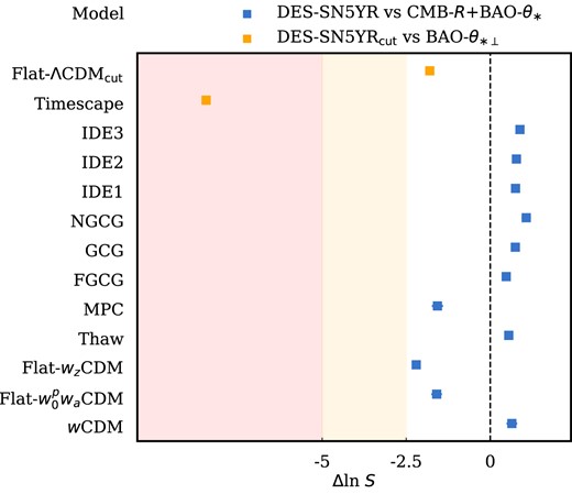
Measurements of |$\Delta$| ln |$~S$| between the DES-SN5YR and the combined CMB- R + BAO-|$\theta _*$| data sets (blue). The modified data sets for the Timescape and Flat-|$\Lambda$|CDM|$_{\mathrm{cut}}$| are shown in orange. The shaded yellow and red regions represent moderate and strong tension, respectively. Note, models already been shown in Section 8.1 to be poor fits to the combined data sets (SCG, DGP, and GAL) have been excluded from the plot for clarity and all had |$\Delta$|ln |$~S \lt \lt -5$|.
9 CONCLUSIONS
The DES Supernova survey is the largest, most homogeneous SN data set to date containing 1635 supernovae combined with 194 existing Low-z SNe Ia. The statistical power of the DES-SN5YR sample allows us to obtain robust and precise constraints on cosmological models beyond |$\Lambda$|CDM.
We first investigated two important areas of the main DES supernova cosmology analysis that are, or may appear to be subject to cosmological dependencies.
We demonstrated that the assumption of a reference cosmology used to generate simulated light curves and perform selection bias corrections to the data results in a bias that is subdominant to statistical uncertainties. For non-standard models, we also show a region of expansion histories where we are confident in our bias corrections. For the next era of SN experiments, the reference cosmology may become a dominating systematic and as a result, we show that an iterative method (where the reference cosmology is updated in a second iteration based on the best-fitting cosmology from the first) is viable and can be employed to reduce this bias.
We demonstrated that the BBC fitting procedure, which uses a fiducial cosmology, is insensitive to that choice of cosmology. We also show that a spline is viable alternative to a fiducial cosmology as it obtains consistent results and may reduce confusion as to the role of the fiducial cosmology in future analyses.
Secondly, we presented constraints on 15 exotic cosmological models using the DES-SN5YR sample alone and after combining the DES-SN5YR with external probes. Using DES-SN5YR alone, we find that all models tested within this work are good fits to the data. This trend continues when we combine the DES-SN5YR with priors from the CMB-R and BAO-|$\theta _*$| except for models that had been previously ruled out. We assessed whether additional parameters invoked in the more complex models are justified given the data by using the Akaike Information Criteria and Suspiciousness. Of the 15 models that we test, we find no strong evidence for or against any of the non-standard models for any of our data combinations. Using the DES-SN5YR alone, the Suspiciousness moderately prefers 3 of the non-standard models along with the fourth order cosmographic model. When combined with the CMB-R and BAO-|$\theta _*$| both the AIC and Suspiciousness agree that 11 models are moderately preferred over Flat-|$\Lambda$|CDM. We show that this is not a result of curvature alone. Our work suggests that additional flexibility in our cosmological models may be required beyond the cosmological constant.
ACKNOWLEDGEMENTS
Author contributions: RCa developed the code, performed the analysis, drafted the manuscript. TMD conceived the idea, guided the project, ran test code, and helped writing. MV contributed to developing part of the analysis, guided the project, and commented on drafts. PS commented on drafts, ran test code, and helped writing. All authors contributed to this paper and/or carried out infrastructure work that made this analysis possible. Highlighted contributions include: Contributed to project development: DB, DS, JF, RK. Contributed to advising and validation: CL, DS, JF, MSa, PA, PW, RK. Construction and validation of the DES-SN5YR Hubble diagram: AC, AM, BP, BS, CL, DB, DS, GT, HQ, JL, LG, MSa, MSm, MSu, MT, PA, PW, RCh, RK SH. Contributed to the internal review process: CL, GFL, JL, LG, MSu, PW, RK. The remaining authors have made contributions to this paper that include, but are not limited to, the construction of DECam and other aspects of collecting the data; data processing and calibration; developing broadly used methods, codes, and simulations; running the pipelines and validation tests; and promoting the science analysis.
TMD, AC, RCa, SH, acknowledge the support of an Australian Research Council Australian Laureate Fellowship (FL180100168) funded by the Australian Government. JF would like to acknowledge Shrihan Agarwal and Yuuki Omori for helpful conversations. MV was partly supported by NASA through the NASA Hubble Fellowship grant HST-HF2-51546.001-A awarded by the Space Telescope Science Institute, which is operated by the Association of Universities for Research in Astronomy, Incorporated, under NASA contract NAS5-26555. LG acknowledges financial support from the Spanish Ministerio de Ciencia e Innovación (MCIN) and the Agencia Estatal de Investigación (AEI) 10.13039/501100011033 under the PID2020-115253GA-I00 HOSTFLOWS project, from Centro Superior de Investigaciones Científicas (CSIC) under the PIE project 20215AT016 and the program Unidad de Excelencia María de Maeztu CEX2020-001058-M, and from the Departament de Recerca i Universitats de la Generalitat de Catalunya through the 2021-SGR-01270 grant. AM is supported by the ARC Discovery Early Career Researcher Award (DECRA) project number DE230100055.
Funding for the DES Projects has been provided by the U.S. Department of Energy, the U.S. National Science Foundation, the Ministry of Science and Education of Spain, the Science and Technology Facilities Council of the United Kingdom, the Higher Education Funding Council for England, the National Center for Supercomputing Applications at the University of Illinois at Urbana-Champaign, the Kavli Institute of Cosmological Physics at the University of Chicago, the Center for Cosmology and Astro-Particle Physics at the Ohio State University, the Mitchell Institute for Fundamental Physics and Astronomy at Texas A&M University, Financiadora de Estudos e Projetos, Fundação Carlos Chagas Filho de Amparo à Pesquisa do Estado do Rio de Janeiro, Conselho Nacional de Desenvolvimento Científico e Tecnológico and the Ministério da Ciência, Tecnologia e Inovação, the Deutsche Forschungsgemeinschaft and the Collaborating Institutions in the Dark Energy Survey.
The Collaborating Institutions are Argonne National Laboratory, the University of California at Santa Cruz, the University of Cambridge, Centro de Investigaciones Energéticas, Medioambientales y Tecnológicas-Madrid, the University of Chicago, University College London, the DES-Brazil Consortium, the University of Edinburgh, the Eidgenössische Technische Hochschule (ETH) Zürich, Fermi National Accelerator Laboratory, the University of Illinois at Urbana-Champaign, the Institut de Ciències de l’Espai (IEEC/CSIC), the Institut de Física d’Altes Energies, Lawrence Berkeley National Laboratory, the Ludwig-Maximilians Universität München and the associated Excellence Cluster Universe, the University of Michigan, NSF’s NOIRLab, the University of Nottingham, The Ohio State University, the University of Pennsylvania, the University of Portsmouth, SLAC National Accelerator Laboratory, Stanford University, the University of Sussex, Texas A&M University, and the OzDES Membership Consortium.
Based in part on observations at Cerro Tololo Inter-American Observatory at NSF’s NOIRLab (NOIRLab Prop. ID 2012B-0001; PI: J. Frieman), which is managed by the Association of Universities for Research in Astronomy (AURA) under a cooperative agreement with the National Science Foundation.
The DES data management system is supported by the National Science Foundation under Grant Numbers AST-1138766 and AST-1536171. The DES participants from Spanish institutions are partially supported by MICINN under grants ESP2017-89838, PGC2018-094773, PGC2018-102021, SEV-2016-0588, SEV-2016-0597, and MDM-2015-0509, some of which include ERDF funds from the European Union. IFAE is partially funded by the CERCA program of the Generalitat de Catalunya. Research leading to these results has received funding from the European Research Council under the European Union’s Seventh Framework Program (FP7/2007-2013) including ERC grant agreements 240672, 291329, and 306478. We acknowledge support from the Brazilian Instituto Nacional de Ciência e Tecnologia (INCT) do e-Universo (CNPq grant 465376/2014-2).
The manuscript has been authored by Fermi Research Alliance, LLC under Contract No. DE-AC02-07CH11359 with the U.S. Department of Energy, Office of Science, Office of High Energy Physics.
Software:numpy (Harris et al. 2020), astropy (Astropy Collaboration 2013, 2018), uncertainties (Lebigot 2009), matplotlib (Hunter 2007), pandas (pandas development team 2020), scipy (Virtanen et al. 2020), snana (Kessler et al. 2009a), pippin (Hinton & Brout 2020), chainconsumer (Hinton 2016), cobaya (Torrado & Lewis 2019; Torrado & Lewis 2021), polychord (Handley et al. 2015a, b), and anesthetic (Handley 2019).
DATA AVAILABILITY
The MCMC and polychord chains along with scripts to reproduce our results in Tables 5 and 6 and contour plots can be found at https://github.com/RyanCamo/DESSN_extensions/.
Footnotes
The BEAMS formalism can equivalently be applied to a spectroscopic SNe Ia sample, by setting the probability of each SN event being type Ia to 1.
Brout et al. (2019) shift the reference cosmology from the best fit by |$\Delta w = -0.05$| and find the difference in distance biases are less than 2 mmag across the entire redshift range.
Note that the fiducial cosmology used within the BBC fit in general can differ from the reference cosmology used to simulate SNe used for bias corrections.
Either a CMB-like prior or a direct matter density prior.
We note that these biases appear larger than those found by Kessler & Scolnic (2017) because they used a strong |$\Omega _{\mathrm{m}}$| prior, which is more similar to what we show on the lower panel of the top-right plot. We discuss why these larger shifts are not concerning below.
Flat-|$\Lambda$|CDM with |$\Omega _{\mathrm{m}}=0.315$|.
The baseline analysis (equation 2) instead uses |$\sigma ^2_{\rm floor}(z_i, c_i, M_{*,i})=\sigma ^2_{\rm scat}(z_i, c_i, M_{*,i})+\sigma ^2_{\rm grey}$| where |$\sigma _{\rm scat}(z_i, c_i, M_{*,i})$| is determined from a model that describes intrinsic brightness fluctuations and |$\sigma _{\rm grey}$| is determined after the BBC fitting process to bring the Hubble diagram reduced |$\chi ^2$| to |$\sim 1$|.
The dressed parameters are defined such that they take numerical values similar to those of cosmological parameters within FLRW models.
We quote |$\frac{1}{2}\Delta$|AIC result, which allows us to use the same scale as the Suspiciousness.
