A fourth-order accurate finite volume scheme for resistive relativistic MHD

ABSTRACT

We present a finite-volume, genuinely fourth-order accurate numerical method for solving the equations of resistive relativistic magnetohydrodynamics in Cartesian coordinates. In our formulation, the magnetic field is evolved in time in terms of face-average values via the constrained-transport method, while the remaining variables (density, momentum, energy, and electric fields) are advanced as cell volume averages. Spatial accuracy employs fifth-order accurate WENO-Z reconstruction from point values (as described in a companion paper) to obtain left and right states at zone interfaces. Explicit flux evaluation is carried out by solving a Riemann problem at cell interfaces, using the Maxwell–Harten–Lax–van Leer with contact wave resolution. Time-stepping is based on the implicit–explicit Runge–Kutta (RK) methods, of which we consider both the third-order strong stability preserving SSP3(4,3,3) and a recent fourth-order additive RK scheme, to cope with the stiffness introduced by the source term in Ampere’s law. Numerical benchmarks are presented in order to assess the accuracy and robustness of our implementation.

magnetic reconnection, MHD, plasmas, relativistic processes, methods: numerical, software: development

1 INTRODUCTION

The investigation of relativistic plasma dynamics holds crucial importance in understanding the complex nature of high-energy astrophysical phenomena. Under typical astrophysical conditions, resistivity remains exceptionally low, and the ideal framework well describes processes occurring on rapid time-scales. Nevertheless, the evolving flow dynamics can cause the formation of local regions with steep gradients, such as current sheets, where the influence of resistivity can no longer be ignored.

It appears then clear the necessity of numerical simulations of astrophysical plasmas beyond the ideal magnetohydrodynamics (MHD) assumptions. Resistive relativistic magnetohydrodynamics (Res-RMHD) is indeed a framework that takes into account the contribution of finite plasma conductivity. In Res-RMHD, the comoving electric field no longer vanishes as in ideal MHD and it is directly proportional to the local current density, which is characterized by a scalar resistivity coefficient denoted as |$\eta$|⁠.

Numerical methods for the solutions of the Res-RMHD equations have been now presented by a number of authors in the context of second-order conservative schemes (see e.g. Komissarov 2007; Palenzuela et al. 2009; Bucciantini & Del Zanna 2013; Dionysopoulou et al. 2013; Mizuno 2013; Miranda-Aranguren, Aloy & Rembiasz 2018; Mignone et al. 2019; Cheong et al. 2022; Nakamura et al. 2023, and references therein) or higher order schemes (Dumbser & Zanotti 2009; Bugli, Del Zanna & Bucciantini 2014; Del Zanna, Bugli & Bucciantini 2014; Tomei et al. 2020).

A delicate aspect of their robust implementation is the stability of the method while dealing with the stiff relaxation term in Ampere’s law, posing very strict constraints for time-explicit calculations. This makes the implementation of Res-RMHD numerical schemes more challenging than their ideal counterpart. In this sense, the employment of implicit–explicit (IMEX) Runge–Kutta (RK; see Pareschi & Russo 2005) represents an effective solution to the problem, allowing larger time-steps to overcome stiffness.

Another important aspect is related to the divergence-free condition and charge conservation that are not automatically fulfilled at the discrete level. To cope with this issue, here we follow an approach similar to Mignone et al. (2019, hereafter Paper I), by adopting the constrained transport (CT) approach to control the divergence of the magnetic field. In the CT formalism (see Evans & Hawley 1988; Balsara & Spicer 1999; Londrillo & del Zanna 2004; Mignone & Del Zanna 2021, and references therein), the magnetic field components are evolved as area-weighted quantities positioned on the faces orthogonal to the corresponding component direction. This ensures that the condition |$\nabla \cdot \nabla \times \boldsymbol {E}=0$| is satisfied also at a discrete level. In Paper I, the CT method has been extended to control the divergence of the electric field as well, thus ensuring a consistent approach for charge conservation. The resulting scheme has shown to be more robust when compared to cell-centred frameworks such as the generalized Lagrange multipliers (Munz et al. 2000; Dedner et al. 2002). In this work, however, we choose to constrain only the magnetic field and evolve the electric field as a zone-centred variable without explicitly enforcing its divergence, simply replacing the charge density with |$\nabla \cdot \boldsymbol {E}$| where needed. As demonstrated later and from extensive testing (not part of this work), we have not found any appreciable evidence of loss of accuracy or stability. Similar conclusions have been reported by Bucciantini & Del Zanna (2013), Del Zanna et al. (2016), and Tomei et al. (2020).

While second-order numerical schemes already provide an effective tool for solving such equations, higher order methods can play a crucial role in the context of Res-RMHD simulations. An increase in overall accuracy and convergence order of the numerical integration, in fact, can significantly decrease the numerical dissipation associated with the scheme’s discretization errors. The benefits of such improvements are twofold. On the one hand, higher order schemes can generally lead to higher computational efficiencies, thus decreasing the computational time required to achieve a given accuracy (Berta et al. 2024). On the other hand, a decrease in numerical dissipation means that we can probe the dynamical impact of more realistic (i.e. lower) values of physical magnetic dissipation, which needs to dominate over the numerical one in any reliable Res-RMHD model (Mattia et al. 2023).

In this paper, we extend the fourth-order accurate finite volume (FV) method described in Berta et al. (2024, hereafter Paper II) to the Res-RMHD equations. Our scheme employs pointwise WENO-Z spatial reconstruction (see Paper II and the original paper by Borges et al. 2008) and either the strong stability preserving (SSP) SSP3(4,3,3) IMEX RK of Pareschi & Russo (2003, 2005) or the more recent IMEX additive Runge-Kutta scheme ARK4(3)7L[2]SA|$_1$| by Kennedy & Carpenter (2019) to achieve, respectively, third- or fourth-order accuracy in time. We refer to Carpenter et al. (2005), Conde et al. (2017), and Boscheri & Pareschi (2021) for other IMEX schemes of high order. Note that the use of pointwise spatial reconstructions is indeed crucial to achieve accuracy beyond the second order when evaluating the implicit stiff source terms within the IMEX formulation, as discussed recently in Boscarino, Russo & Semplice (2018).

The rest of the paper is structured as follows. In Section 2, we review the fundamental equations of the Res-RMHD framework. In Section 3, our fourth-order FV–CT method is illustrated, and in Section 4, we assess the robustness of the algorithm through extensive numerical benchmarking. Results are summarized in Section 5.

2 RESISTIVE RELATIVISTIC MHD EQUATIONS

When dealing with relativistic plasmas, it is convenient to start from the appropriate set of covariant equations. In the (single fluid) MHD approximation, these consist of the Maxwell equations:

$$\begin{eqnarray} \nabla _\mu F^{\mu \nu } = -J^\nu , \qquad \nabla _\mu F^{*\mu \nu } = 0, \end{eqnarray}$$

(1)

where |$F^{\mu \nu }$|⁠, |$F^{*\mu \nu }$|⁠, and |$J^\mu$| are, respectively, the Faraday tensor, its dual, and the four-current density, and in the conservation laws for mass and total (gas and electromagnetic fields) energy–momentum:

$$\begin{eqnarray} \nabla _\mu (\rho u^\mu) = 0 ,\qquad \nabla _\mu T^{\mu \nu } \equiv \nabla _\mu (T^{\mu \nu }_\mathrm{gas} + T^{\mu \nu }_\mathrm{em}) = 0, \end{eqnarray}$$

(2)

where |$\rho$| is the rest-mass density, |$u^\mu$| is the four-velocity of the fluid, and |$T^{\mu \nu }$| is the total energy–momentum tensor. The two contributions are, respectively,

$$\begin{eqnarray} T^{\mu \nu }_\mathrm{gas} & = & \rho h \, u^\mu u^\nu + pg^{\mu \nu }, \\T^{\mu \nu }_\mathrm{em} & = & F^\mu _{\, \, \, \lambda }F^{\nu \lambda }-\frac{1}{4}(F_{\lambda \kappa }F^{\lambda \kappa }) g^{\mu \nu }, \end{eqnarray}$$

(3)

where h, |$\varepsilon$|⁠, and p are, respectively, the gas specific enthalpy, energy density, and pressure, as measured in the fluid rest frame and related by |$\rho h = \varepsilon + p$|⁠. These thermodynamic quantities must be also connected by an equation of state (EoS), for instance, given in the form |$h=h(\rho ,p)$|⁠.

It is convenient to express the Faraday tensor and its dual in terms of the four-velocity and the magnetic |$b^\mu$| and electric |$e^\mu$| fields measured in the fluid rest frame:

$$\begin{eqnarray} F^{\mu \nu } & = & u^\mu e^\nu -u^\nu e^\mu + \epsilon ^{\mu \nu \lambda \kappa }b_\lambda u_\kappa , \\F^{*\mu \nu } & = & u^\mu b^\nu -u^\nu b^\mu -\epsilon ^{\mu \nu \lambda \kappa }e_\lambda u_\kappa , \end{eqnarray}$$

(4)

where |$\epsilon ^{\mu \nu \lambda \kappa }$| represents the Levi-Civita pseudo-tensor. Ideal relativistic MHD is obtained by assuming a vanishing electric field in the frame comoving with the fluid, while in the resistive case we will assume a simple Ohmic relation

$$\begin{eqnarray} e^\mu = \eta j^\mu , \end{eqnarray}$$

(5)

where |$j^\mu = J^\mu + (J^\nu u_\nu) u^\mu$| is the current density measured in the fluid frame and |$\eta$| is the resistivity coefficient, supposed to be a scalar for the sake of simplicity.

Assuming from now on a Minkowski flat space–time and splitting time and space, it is convenient to write the fluid velocity as

$$\begin{eqnarray} u^\mu = \left(\sqrt{1 + u^2},\boldsymbol {u}\right) \equiv (\gamma ,\gamma \boldsymbol {v}), \end{eqnarray}$$

(6)

where |$\boldsymbol {v}$| is the usual three-dimensional velocity of the fluid measured in the laboratory frame and |$\gamma$| the associated Lorentz factor, while the electromagnetic fields can be split as

$$\begin{eqnarray} \begin{array}{lll}e^\mu & = & (\bf {u}\cdot \bf {E}, \, \gamma \, \bf {E} + \bf {u}\times \bf {B}), \\b^\mu & = & (\bf {u}\cdot \bf {B}, \, \gamma \, \bf {B}-\bf {u}\times \bf {E}), \end{array} \end{eqnarray}$$

(7)

where |$\boldsymbol {E}$| and |$\boldsymbol {B}$| are the usual electric and magnetic fields measured in the laboratory frame. The four-current can be also split

$$\begin{eqnarray} J^\mu = (q,\boldsymbol {J}) = (q , \, q\boldsymbol {v} + \eta ^{-1}\tilde{\boldsymbol {E}}), \end{eqnarray}$$

(8)

in which q is the charge density measured in the laboratory frame and |$\boldsymbol {J}$| the spatial current density, with

$$\begin{eqnarray} \tilde{\bf {E}} \equiv \gamma \bf {E} + \bf {u}\times \bf {B}-(\bf {E}\cdot \bf {u})\bf {v} \Rightarrow \tilde{\bf {E}} = \eta (\bf {J}- {\mathrm{q}}\bf {v}), \end{eqnarray}$$

(9)

where equations (5) and (7) have been used. Given the above spatial vectors, Maxwell’s system is written in the usual way, a couple of evolutionary equations

$$\begin{eqnarray} \frac{\partial \boldsymbol {B}}{\partial t} + \nabla \times \boldsymbol {E} = 0 , \qquad \frac{\partial \boldsymbol {E}}{\partial t} -\nabla \times \boldsymbol {B} = - \boldsymbol {J}, \end{eqnarray}$$

(10)

and a couple of non-evolutionary constraints

$$\begin{eqnarray} \nabla \cdot \boldsymbol {B} = 0 , \qquad \nabla \cdot \boldsymbol {E} = q, \end{eqnarray}$$

(11)

and we use the latter, Gauss’s law, to define the charge density q.

The final system of Res-RMHD is retrieved by splitting the covariant equations (2), and by the first couple of Maxwell’s equations (10). We obtain 11 evolution equations that may be written in the form of a set of conservation laws with source terms

$$\begin{eqnarray} \frac{\partial U}{\partial t} = -\nabla \cdot \boldsymbol{\sf F}(U) + S_{\rm e} (U) + S(U), \end{eqnarray}$$

(12)

where

$$\begin{eqnarray} U = \begin{pmatrix}D \\m_i \\{\cal E} \\B_i \\E_i \end{pmatrix}, \quad \boldsymbol{\sf F}_j = \begin{pmatrix}\rho u_j \\\rho h u_i u_j -E_iE_j -B_iB_j + p_\mathrm{tot}\delta _{ij} \\m_j \\\varepsilon ^{ijk} E_k \\-\varepsilon ^{ijk} B_k \end{pmatrix}, \end{eqnarray}$$

(13)

with |$\varepsilon ^{ijk}$| is the three-dimensional Levi-Civita symbol. Here the mass density |$D=\rho \gamma$|⁠, the total momentum density |$\boldsymbol {m}= D h\, \boldsymbol {u} + \boldsymbol {E}\times \boldsymbol {B}$|⁠, and the total energy density |${\cal E}=D h\gamma -p + u_\mathrm{em}$| (all measured in the laboratory frame) are the so-called conserved variables, where |$u_\mathrm{em} = (E^2 + B^2)/2$| is the electromagnetic energy density, and |$p_\mathrm{tot}=p+u_\mathrm{em}$| is the total pressure. These variables are expressed in terms of the primitive variables |$\rho$|⁠, |$\boldsymbol {v}$|⁠, and p. Notice that the electric and magnetic fields |$\boldsymbol {E}$| and |$\boldsymbol {B}$| act as both conserved and primitive variables.

The source term is non-zero only in the equation for |$\boldsymbol {E}$| and it contains the spatial current density |$\boldsymbol {J}$| in equation (8). This is split, for computational purposes, into standard and stiff (⁠|${\propto} 1/\eta$|⁠) contributions, so that the source terms |$S_{\rm e}$| and S in equation (12) are given by

$$\begin{eqnarray} S_{\rm e} = \begin{pmatrix}0_{\times 8} \\-q v_i \end{pmatrix} ,\quad S = \frac{1}{\eta } \begin{pmatrix}0_{\times 8} \\-\tilde{E}_i \end{pmatrix}, \end{eqnarray}$$

(14)

where |$\tilde{\boldsymbol {E}}$| is defined in equation (9). Numerical stiffness is obviously given by the fact that the resistivity coefficient |$\eta$| is negligible in real astrophysical plasmas, and finite but very small in computational applications, so the term S can be very large and special care should be adopted for the evolution of the electric field (the terms R and S will be treated differently in the numerical time evolution of U).

We recall that in ideal MHD, i.e. assuming the limit |$\eta \rightarrow 0$|⁠, this latter equation is not evolved at all, the current does not need to be computed, and the electric field is a derived quantity, simply given by |$\boldsymbol {E} = - \boldsymbol {v}\times \boldsymbol {B}$|⁠, so that |$\tilde{\boldsymbol {E}} = 0$|⁠.

3 NUMERICAL METHOD

3.1 Basic discretization

We employ a Cartesian coordinate system with axes represented by the unit vectors |$\hat{\boldsymbol {e}}_x = (1,0,0)$|⁠, |$\hat{\boldsymbol {e}}_y =(0,1,0)$|⁠, and |$\hat{\boldsymbol {e}}_z =(0,0,1)$|⁠, uniformly discretized into a regular mesh with coordinate spacing |$\Delta x$|⁠, |$\Delta y$|⁠, and |$\Delta z$|⁠. We will frequently use the notation |${\boldsymbol{c}} = (i,j,k)$| as a shorthand to identify a single computational cell centred at |$(x_i, y_j, z_k)$| and delimited by the six interfaces orthogonal to the coordinate axis centred, respectively, at |$(x_{i\pm \frac{1}{2}},\, y_j,\, z_k)$|⁠, |$(x_i, y_{j\pm \frac{1}{2}}, z_k)$|⁠, and |$(x_i, y_j, z_{k\pm \frac{1}{2}})$|⁠. The grid interfaces location will be shorthanded with

$$\begin{eqnarray} {\boldsymbol {x}_{\rm f}}& \equiv & \left(i+\frac{1}{2}, j, k\right), \\{\boldsymbol {y}_{\rm f}}& \equiv & \left(i, j+\frac{1}{2}, k\right), \\{\boldsymbol {z}_{\rm f}}& \equiv & \left(i, j, k+\frac{1}{2}\right) . \end{eqnarray}$$

(15)

Likewise, we define the location of the cell edges as

$$\begin{eqnarray} {\boldsymbol{x}_{\rm e}}& \equiv & \left(i,j+\frac{1}{2},k+\frac{1}{2}\right), \\{\boldsymbol{y}_{\rm e}}& \equiv & \left(i+\frac{1}{2},j,k+\frac{1}{2}\right), \\{\boldsymbol{z}_{\rm e}}& \equiv & \left(i+\frac{1}{2},j+\frac{1}{2},k\right) . \end{eqnarray}$$

(16)

Integrating the original partial differential equation (PDE; equation 12) over a cell volume for |$U=\lbrace D, \boldsymbol {m}, \mathcal {E}, \boldsymbol {E} \rbrace$| gives the semidiscrete form

$$\begin{eqnarray} \frac{\mathrm{ d}\left\langle {U} \right\rangle _{ {\boldsymbol{c}} }}{\mathrm{ d}t} = \hat{R}_ {\boldsymbol{c}} + \left\langle {S } \right\rangle _ {\boldsymbol{c}}, \end{eqnarray}$$

(17)

where |$\left\langle {U} \right\rangle _{ {\boldsymbol{c}} }$| denotes the volume average of the corresponding conserved quantity, |$\left\langle {S} \right\rangle _ {\boldsymbol{c}}$| is the stiff part of the source term (second term in equation 14), while

$$\begin{eqnarray} \displaystyle \hat{R}_ {\boldsymbol{c}} &=&\displaystyle -\left(\frac{ \hat{F}_{x, {\boldsymbol {x}_{\rm f}} }-\hat{F}_{x, {\boldsymbol {x}_{\rm f}} -\hat{\boldsymbol {e}}_x} }{\Delta x}\right) -\left(\frac{ \hat{F}_{y, {\boldsymbol {y}_{\rm f}} }-\hat{F}_{y, {\boldsymbol {y}_{\rm f}} -\hat{\boldsymbol {e}}_y} }{\Delta y}\right) \\&&\displaystyle -\left(\frac{ \hat{F}_{z, {\boldsymbol {z}_{\rm f}} }-\hat{F}_{z, {\boldsymbol {z}_{\rm f}} -\hat{\boldsymbol {e}}_z} }{\Delta z}\right) + \left\langle {S_{\rm e}} \right\rangle _ {\boldsymbol{c}} \end{eqnarray}$$

(18)

is the explicit right-hand side including surface flux contributions plus the volume average of the explicit source term |$S_{\rm e}$| (first term in equation 14) whose only non-vanishing component is the |$q\boldsymbol {v}$| term in the electric field update.

In equation (18), |$\hat{F}_{x, {\boldsymbol {x}_{\rm f}} }$| (and likewise |$\hat{F}_{y, {\boldsymbol {y}_{\rm f}} }$| and |$\hat{F}_{z, {\boldsymbol {z}_{\rm f}} }$|⁠) represents the surface-integrated numerical flux across an x-face, i.e.

$$\begin{eqnarray} \hat{F}_{x, {\boldsymbol {x}_{\rm f}} } = \frac{1}{\Delta y\Delta z} \int F_{x, {\boldsymbol {x}_{\rm f}} } \, \mathrm{ d}y\, \mathrm{ d}z, \end{eqnarray}$$

(19)

which has to be computed with a high-order quadrature rule. Expressions for the y- and z-directions are obtained in a similar fashion.

Magnetic field variables are treated as staggered quantities and are evolved using the integral form of Faraday’s law (the first part in equation 10) and direct application of Stokes’ theorem (see sections 2, 3, and 4 of Paper II for more details). Thus, if |$\hat{B}_{x, {\boldsymbol {x}_{\rm f}} }$|⁠, |$\hat{B}_{y, {\boldsymbol {y}_{\rm f}} }$|⁠, and |$\hat{B}_{z, {\boldsymbol {z}_{\rm f}} }$| are the surface-averaged components of |$\boldsymbol {B}$| lying, respectively, on the x-, y-, and z-interfaces, the CT (see Yee 1966; Brecht et al. 1981; Evans & Hawley 1988; Balsara & Spicer 1999) algorithm entails the following discrete update:

$$\begin{eqnarray} \displaystyle \frac{\mathrm{ d}\hat{B}_{x, {\boldsymbol {x}_{\rm f}} }}{\mathrm{ d}t} &=& \displaystyle -\left(\frac{\bar{E}_{z, {\boldsymbol{z}_{\rm e}} }-\bar{E}_{z, {\boldsymbol{z}_{\rm e}} -\hat{\boldsymbol {e}}_y}}{\Delta y} -\frac{\bar{E}_{y, {\boldsymbol{y}_{\rm e}} }-\bar{E}_{y, {\boldsymbol{y}_{\rm e}} -\hat{\boldsymbol {e}}_z}}{\Delta z} \right) , \\\displaystyle \frac{\mathrm{ d}\hat{B}_{y, {\boldsymbol {y}_{\rm f}} }}{\mathrm{ d}t} &=& \displaystyle -\left(\frac{\bar{E}_{x, {\boldsymbol{x}_{\rm e}} }-\bar{E}_{x, {\boldsymbol{x}_{\rm e}} -\hat{\boldsymbol {e}}_z}}{\Delta z} -\frac{\bar{E}_{z, {\boldsymbol{z}_{\rm e}} }-\bar{E}_{z, {\boldsymbol{z}_{\rm e}} -\hat{\boldsymbol {e}}_x}}{\Delta x} \right) , \\\displaystyle \frac{\mathrm{ d}\hat{B}_{z, {\boldsymbol {z}_{\rm f}} }}{\mathrm{ d}t} &=& \displaystyle -\left(\frac{\bar{E}_{y, {\boldsymbol{y}_{\rm e}} }-\bar{E}_{y, {\boldsymbol{y}_{\rm e}} -\hat{\boldsymbol {e}}_x}}{\Delta x} -\frac{\bar{E}_{x, {\boldsymbol{x}_{\rm e}} }-\bar{E}_{x, {\boldsymbol{x}_{\rm e}} -\hat{\boldsymbol {e}}_y}}{\Delta y} \right) . \end{eqnarray}$$

(20)

In the previous expressions, we have denoted the line-averaged electric field (electromotive force or emf) at zone edges with |$\bar{E}_{x, {\boldsymbol{x}_{\rm e}} }$|⁠, |$\bar{E}_{y, {\boldsymbol{y}_{\rm e}} }$|⁠, and |$\bar{E}_{z, {\boldsymbol{z}_{\rm e}} }$|⁠. The actual computation of the emf is detailed in Section 3.7.

Finally, it is worth to remind that in the presented fourth-order scheme only magnetic field components are evolved as surface average, while electric field (unlike Paper I) is treated as a zone-centred variable rather than in a staggered fashion.

3.2 Temporal update

Equations (17) and (20) are evolved in time using IMEX RK schemes, for stiffly accurate (SA) computations. When applied to equation (17), an IMEX RK scheme can be expressed following the general formulation of Ascher, Ruuth & Spiteri (1997) and Pareschi & Russo (2005), yielding

$$\begin{eqnarray} \left\langle {U} \right\rangle _ {\boldsymbol{c}} ^{(k)} &=& \displaystyle \left\langle {U} \right\rangle _ {\boldsymbol{c}} ^n + \Delta t\sum _{j=1}^{k-1}\tilde{a}_{kj} \hat{R}_ {\boldsymbol{c}} + \Delta t\sum _{j=1}^{k}{a}_{kj}\left\langle {S} \right\rangle _ {\boldsymbol{c}} ^{(j)}, \\\left\langle {U} \right\rangle _ {\boldsymbol{c}} ^{n+1} &=& \displaystyle \left\langle {U} \right\rangle _ {\boldsymbol{c}} ^n + \Delta t\sum _{j=1}^{\nu }\tilde{w}_{j}\hat{R}_ {\boldsymbol{c}} ^{(j)} + \Delta t\sum _{j=1}^{\nu }{w}_{j}\left\langle {S} \right\rangle _ {\boldsymbol{c}} ^{(j)}, \end{eqnarray}$$

(21)

where |$\nu$| is the number of integration stages, |$\tilde{A}$| is a |$\nu \times \nu$| lower triangular matrix (⁠|$\tilde{a}_{ij} = 0$|⁠, |$\forall j \ge i$|⁠) enclosing the coefficients of the explicit right-hand side |$\hat{R}_ {\boldsymbol{c}}$| (equation 18 or the right-hand side of equation 20), while |$A=(a_{ij})$| is also a |$\nu \times \nu$| matrix including the coefficients for the implicit part of the right-hand side, |$S^{(j)}$|⁠. We recall that the use of a diagonally implicit RK solver guarantees an explicit evaluation of the non-stiff terms and implicit evaluation only for the diagonally stiff terms.

The final stage is always explicit and it is expressed in terms of the coefficient vectors |$\tilde{w} = (\tilde{w}_1, \ldots, \tilde{w}_\nu)^\mathrm{ T}$| and |$w = (w_1, \ldots , w_\nu)^\mathrm{ T}$|⁠. IMEX RK schemes are conveniently represented with a double tableau in the usual Butcher notation,

$$\begin{eqnarray} \qquad \qquad \qquad \qquad \begin{array}{c|c}\tilde{c} & \tilde{A} \\\hline \\& \tilde{w}^\mathrm{ T} \end{array} \qquad \begin{array}{c|c}c & A \\\hline \\& w^\mathrm{ T} \end{array}, \end{eqnarray}$$

(22)

where the coefficients |$\tilde{c}$| and c refer to the treatment of non-autonomous systems and are defined as

$$\begin{eqnarray} \qquad \qquad \qquad \qquad \tilde{c}_i = \sum _{j = 1}^{i-1} \tilde{a}_{ij} , \quad c_i = \sum _{j = 1}^{i} a_{ij} . \end{eqnarray}$$

(23)

In this paper, we consider two IMEX time-stepping methods: (i) the third-order accurate IMEX SSP3(4,3,3) scheme of Pareschi & Russo (2005) (with four implicit and three explicit stages) and (ii) the fourth-order IMEX ARK4(3)7L[2]SA|$_1$| of Kennedy & Carpenter (2019) (hereafter ARK4), which is L-stable, SA with seven stages. The explicit coefficients of both methods can be found in Appendix A.

From an algorithmic viewpoint, during the explicit–implicit update we found more convenient to separate the explicit contributions (acting on volume averages) from the implicit part, which, in our formulation, will be operated on pointwise values. For the generic kth stage in equation (21), we therefore act as follows:

$$\begin{eqnarray} \left\langle {U} \right\rangle _ {\boldsymbol{c}} ^{(k*)} &=& \displaystyle \left\langle {U} \right\rangle _ {\boldsymbol{c}} ^n + \Delta t\sum _{j=1}^{k-1}\left(\tilde{a}_{kj} \hat{R}_ {\boldsymbol{c}} + {a}_{kj}\left\langle {S} \right\rangle _ {\boldsymbol{c}} ^{(j)}\right), \\U^{(k)}_ {\boldsymbol{c}} &=& U^{(k*)}_{ {\boldsymbol{c}} } + \Delta t a_{kk} S^{(k)}_ {\boldsymbol{c}}, \end{eqnarray}$$

(24)

where the former step |$(k*)$| is explicit, while the latter |$(k)$| is implicit. The algorithm is summarized in Section 3.10.

3.3 Point value recovery of primitive variables

Our algorithm starts with the zone-averaged value of the solution |$\left\langle {U} \right\rangle _{ {\boldsymbol{c}} }$| inside a cell and the face-averaged values of the staggered components of the magnetic field |$\hat{\boldsymbol {B}}$|⁠. At the very first step, we require the point value of the solution at the cell centre. Following Paper II, this operation may be carried out using the Laplacian operator,

$$\begin{eqnarray} U_ {\boldsymbol{c}} = \left(1-\frac{\Delta }{24}\right) \left\langle {U} \right\rangle _ {\boldsymbol{c}} + O(h^4), \end{eqnarray}$$

(25)

where |$\Delta$| is the Laplacian operator first introduced in the context of high-order methods by McCorquodale & Colella (2011), i.e.

$$\begin{eqnarray} \Delta \left\langle {U} \right\rangle _{ {\boldsymbol{c}} } \equiv \left(\Delta ^{x} + \Delta ^{y} + \Delta ^{z}\right)\left\langle {U} \right\rangle _ {\boldsymbol{c}}, \end{eqnarray}$$

(26)

where e.g.

$$\begin{eqnarray} \Delta ^{x} \left\langle {U} \right\rangle _{ {\boldsymbol{c}} } = \displaystyle \left(\left\langle {U} \right\rangle _{ {\boldsymbol{c}} -\hat{\boldsymbol {e}}_x}-2\left\langle {U} \right\rangle _{ {\boldsymbol{c}} } + \left\langle {U} \right\rangle _{ {\boldsymbol{c}} + \hat{\boldsymbol {e}}_x} \right), \end{eqnarray}$$

(27)

and similarly of the y- and z-directions. Note that this step applies only to cell-centred quantities, i.e. lab density, momentum, energy, and electric fields. For the magnetic field, instead, one has to first recover its point values at face centres using only the transverse Laplacian, so that

$$\begin{eqnarray} \displaystyle B_{x, {\boldsymbol {x}_{\rm f}} } &=& \left(1-\frac{\Delta ^y+\Delta ^z}{24}\right)\hat{B}_{x, {\boldsymbol {x}_{\rm f}} } , \\\displaystyle B_{y, {\boldsymbol {y}_{\rm f}} } &=& \left(1-\frac{\Delta ^z+\Delta ^x}{24}\right)\hat{B}_{y, {\boldsymbol {y}_{\rm f}} } , \\\displaystyle B_{z, {\boldsymbol {z}_{\rm f}} } &=& \left(1-\frac{\Delta ^x+\Delta ^y}{24}\right)\hat{B}_{z, {\boldsymbol {z}_{\rm f}} } . \end{eqnarray}$$

(28)

Then, following Felker & Stone (2018), the pointwise value of the magnetic field at the cell centre is obtained using an unlimited high-order interpolation, i.e.

$$\begin{eqnarray} \displaystyle B_{x, c} &=& - \frac{1}{16}(B_{x, {\boldsymbol {x}_{\rm f}} +\hat{\boldsymbol {e}}_x} + B_{x, {\boldsymbol {x}_{\rm f}} -2\hat{\boldsymbol {e}}_x}) + \frac{9}{16}(B_{x, {\boldsymbol {x}_{\rm f}} } + B_{x, {\boldsymbol {x}_{\rm f}} -\hat{\boldsymbol {e}}_x}) , \\\displaystyle B_{y, c} &=& - \frac{1}{16}(B_{y, {\boldsymbol {y}_{\rm f}} +\hat{\boldsymbol {e}}_y} + B_{y, {\boldsymbol {y}_{\rm f}} -2\hat{\boldsymbol {e}}_y}) + \frac{9}{16}(B_{y, {\boldsymbol {y}_{\rm f}} } + B_{y, {\boldsymbol {y}_{\rm f}} -\hat{\boldsymbol {e}}_y}) , \\\displaystyle B_{z, c} &=& - \frac{1}{16}(B_{z, {\boldsymbol {z}_{\rm f}} +\hat{\boldsymbol {e}}_z} + B_{z, {\boldsymbol {z}_{\rm f}} -2\hat{\boldsymbol {e}}_z}) + \frac{9}{16}(B_{z, {\boldsymbol {z}_{\rm f}} } + B_{z, {\boldsymbol {z}_{\rm f}} -\hat{\boldsymbol {e}}_z}) . \end{eqnarray}$$

(29)

Now that all conservative variables are available at zone centres as point values, we convert them to primitive variables, i.e. |$V_ {\boldsymbol{c}} = {\mathcal {V}}(U_ {\boldsymbol{c}})$|⁠. The conversion between conservative and primitive variables cannot be written in closed analytical form as it requires the inversion of a non-linear function. Differently from Paper I, here we prefer to follow an approach similar to that of Palenzuela et al. (2009), which consists of subtracting the electromagnetic contributions from momentum and energy densities and then resorting to a standard relativistic hydro inversion scheme to find the pressure. In our implementation, we employ the root solver of Mignone, Plewa & Bodo (2005, see also section 2 in Mignone & Bodo 2005) that can be extended to different EoSs.

Note that equation (25) may produce unphysical states in the presence of sharp gradients and in regions of rapidly changing profiles. A limiting strategy to identify troubled cells is indeed necessary before operating any conversion operation to maintain numerical stability. We discuss our fallback approach in Section 3.9 of this paper, while the reader may consult section 3.4 of Paper II for a full description.

3.4 Implicit update of pointwise quantities

During the implicit part of our update (see the second part in equation 24), we operate directly on the point value of the electric field vector:

$$\begin{eqnarray} \boldsymbol {E} = \boldsymbol {E}^{*} - \frac{1}{\tilde{\eta }}\left[\gamma \boldsymbol {E} + \boldsymbol {u}\times \boldsymbol {B}-(\boldsymbol {E}\cdot \boldsymbol {u})\boldsymbol {v}\right], \end{eqnarray}$$

(30)

where, by analogy with equation (24), we identify |$\boldsymbol {E}^{*} \equiv \boldsymbol {E}^{(k*)}$| (available from the last explicit stage) and |$\tilde{\eta }=\eta /(a_{kk}\Delta t)$|⁠, which is now a non-dimensional quantity. The previous equation provides a relation between the electric field |$\boldsymbol {E}$| and the four-velocity |$\boldsymbol {u}$|⁠. Using

$$\begin{eqnarray} \boldsymbol {E}\cdot \boldsymbol {u} = \frac{\tilde{\eta }\gamma }{1+\tilde{\eta }\gamma } (\boldsymbol {E}^{*}\cdot \boldsymbol {u}), \end{eqnarray}$$

(31)

we can rewrite equation (30) as an explicit function |$\boldsymbol {E}\equiv \boldsymbol {E}(\boldsymbol {u})$|⁠:

$$\begin{eqnarray} (\tilde{\eta }+\gamma) \boldsymbol {E}(\boldsymbol {u})= \tilde{\eta }\, \boldsymbol {E}^{*} - \boldsymbol {u}\times \boldsymbol {B} + \frac{\tilde{\eta }}{1 + \tilde{\eta }\gamma }(\boldsymbol {E}^{*}\cdot \boldsymbol {u})\boldsymbol {u} , \end{eqnarray}$$

(32)

where |$\gamma = \sqrt{1+u^2}$|⁠.

Note that the four-velocity is not a conservative variable and it must be derived from the set of conserved variables U. Since momentum does not change during the implicit step, we use the implicit relation

$$\begin{eqnarray} \boldsymbol {f}(\boldsymbol {u}) = \boldsymbol {m}-\Big (Dh(\boldsymbol {u})\boldsymbol {u} + \boldsymbol {E}(\boldsymbol {u})\times \boldsymbol {B}\Big) = \boldsymbol {0} \end{eqnarray}$$

(33)

to derive |$\boldsymbol {u}$|⁠, as in Paper I. Note also that D and |$\boldsymbol {B}$| are held constant during this step. Following Bucciantini & Del Zanna (2013), we adopt a Newton–Broyden root-finding method to derive the four-velocity (and the other primitive variables) from the set of conserved variables. Additionally, we refer the reader to Mattia et al. (2023) for a generalization of the Taub EoS (Mignone et al. 2005) and to Tomei et al. (2020) for a more comprehensive treatment of the dynamo term in Ohm’s law along with for any space–time metric in general relativity. The iterative multidimensional Newton–Brodyen algorithm can be sketched as follows:

At the beginning of any step |$\kappa =0,1,2, \ldots$|⁠, use equation (32) to obtain |$\boldsymbol {E}=\boldsymbol {E}(\boldsymbol {u})$|⁠. When |$\kappa = 0$|⁠, an initial guess for the four-velocity is needed: if |$\tilde{\eta } \gt 1$|⁠, employ the value provided at the current time level, otherwise reckon that obtained from the ideal RMHD equations.
Given |$\boldsymbol {u}^{(\kappa)}$| and |$\boldsymbol {E}^{(\kappa)}$|⁠, compute |$\boldsymbol {f}^{(\kappa)} \equiv \boldsymbol {f}(\boldsymbol {u}^{(\kappa)})$| from the conservation of the total momentum density:
$$\begin{eqnarray} \boldsymbol {f}^{(\kappa)} = \boldsymbol {m}-\Big [Dh(\boldsymbol {u})\boldsymbol {u} + \boldsymbol {E}(\boldsymbol {u})\times \boldsymbol {B}\Big ]^{(\kappa)}. \end{eqnarray}$$
(34)
Notice that the laboratory density, magnetic field, total energy, and conserved momentum remain constant during this iteration scheme. Equation (34) represents a set of three non-linear equations to be solved for |$\boldsymbol {u}^{(\kappa)}$|⁠. Thermodynamics quantities are also written as functions of the four-velocity; for an ideal gas law one finds
$$\begin{eqnarray} h(\boldsymbol {u}) = 1 + \Gamma _1 \frac{p\gamma }{D}, \end{eqnarray}$$
(35)
with |$\Gamma _1=\Gamma /(\Gamma -1)$| (⁠|$\Gamma = 4/3$| for relativistically hot plasmas), and, from the conservation of the total energy, the pressure is derived as
$$\begin{eqnarray} p(\boldsymbol {u}) = \frac{\mathcal {E}-D\gamma - (E^2 + B^2)/2}{\Gamma _1\gamma ^2-1}. \end{eqnarray}$$
(36)
Using the Jacobian |$\boldsymbol{\sf J}=\partial \boldsymbol {f}/\partial \boldsymbol {u}$|⁠, obtain an improved guess of the four-velocity through
$$\begin{eqnarray} \boldsymbol {u}^{(\kappa +1)} = \boldsymbol {u}^{(\kappa)}-\left(\mathsf {J}^{(\kappa)}\right)^{-1}\boldsymbol {f}^{(\kappa)}, \end{eqnarray}$$
(37)
with the explicit form of the Jacobian being
$$\begin{eqnarray} {\boldsymbol{\sf J}}_{ij} \equiv \frac{\partial f_i}{\partial u_j} = -Dh\, \delta _{ij}-D\, u_i\frac{\partial h}{\partial u_j} -\epsilon _{ilm}\frac{\partial E_l}{\partial u_j} B_m. \end{eqnarray}$$
(38)
The derivatives of h and |$\boldsymbol {E}$| are given by
$$\begin{eqnarray} D \frac{\partial h}{\partial u^j} = - \frac{\Gamma _1}{\gamma ^2\Gamma _1-1}\left[(\gamma h D + p) v_j + \gamma E_i \frac{\partial E_i}{\partial u_j} \right], \end{eqnarray}$$
(39)
given the relation |$\partial \gamma /\partial u_j = u_j/\gamma = v_j$|⁠, and, from equation (32), by
$$\begin{eqnarray} \begin{array}{l}\displaystyle (\tilde{\eta } + \gamma) \frac{\partial E_i}{\partial u_j} = - E_i v_j-\epsilon _{ijk} B_k \\\displaystyle \quad + \frac{\tilde{\eta }}{1 + \tilde{\eta }\gamma } \left[u_i E^{*}_j + (\boldsymbol {E}^{*}\cdot \boldsymbol {u}) \left(\delta _{ij} -\frac{\tilde{\eta }}{1 + \tilde{\eta }\gamma } u_iv_j \right) \right], \end{array} \end{eqnarray}$$
(40)
which can be also compared to the Jacobian presented in Tomei et al. (2020) (for a vanishing dynamo coefficient |$\xi =0$|⁠).
Exit the iteration cycle if the error is less than some prescribed accuracy |$|\boldsymbol {f}^{(\kappa)}|\lt \epsilon$|⁠, otherwise go back to step (i) and let |$\kappa \rightarrow \kappa +1$|⁠. For standard applications, our algorithm converges in |$2\!-\!5$| iterations given a relative tolerance of |$10^{-11}$|⁠.

The above procedure is to be implemented at the beginning of all IMEX substeps at cell centres using pointwise quantities. Furthermore, it automatically operates the conversion from conservative to primitive variables, which are then readily available for reconstruction at cell interfaces and flux computation. For this reason, this procedure must be extended also to a layer of ghost zones (e.g. three for a five-point stencil reconstruction) in order to avoid extra communication at the end of the implicit step.

3.5 Point value reconstruction of primitive variables

Reconstruction at interfaces is operated directly on the function point values rather than on the one-dimensional average quantities as first introduced by Paper II. In the following paragraphs, we summarize the pointwise fifth-order weighted essentially non-oscillatory scheme of Borges et al. (WENO-Z; see Borges et al. 2008).

The interface value presented in equation (23) of Paper II at |$x=x_{i+\frac{1}{2}}$| is computed as the convex combination of third-order accurate interface values built on the three possible three-point substencils |$\lbrace i-2,i-1,i\rbrace$|⁠, |$\lbrace i-1,i,i+1\rbrace$|⁠, and |$\lbrace i,i+1,i+2\rbrace$|⁠, i.e.

$$\begin{eqnarray} \displaystyle V^L_{i+\frac{1}{2}} & = & \displaystyle \omega _0 \frac{3V_{i-2}-10V_{i-1} + 15V_i}{8} \\& + & \displaystyle \omega _1 \frac{-V_{i-1} + 6V_{i} + 3V_{i+1}}{8} \\& + & \displaystyle \omega _2 \frac{3V_{i} + 6V_{i+1}-V_{i+2}}{8} , \end{eqnarray}$$

(41)

with |$\lbrace V_{i\pm 2}, V_{i\pm 1}, V_{i} \rbrace$| point values. The weights |$\omega _l$|⁠, for |$l=\lbrace 0,1,2\rbrace$|⁠, are defined as

$$\begin{eqnarray} \omega _l = \frac{\alpha _l}{\sum _{m} \alpha _m}, \alpha _l = d_l\left(1+ \frac{|\beta _0-\beta _2|}{\beta _l+\epsilon }\right) . \end{eqnarray}$$

(42)

Here |$d_l = \lbrace d_0 = 1/16, d_1 = 5/8, d_2 = 5/16 \rbrace$| denotes the optimal weights that reckon the fifth-order accurate approximation of equation (23) of Paper II, |$\epsilon = 10^{-40}$| is a small number avoiding division by zero, and |$\beta _l$| are the smoothness indicators (equation 26 of Paper II). A detailed description of pointwise reconstructions is presented in section 3 of Paper II.

3.6 Riemann solver and flux computation

The integrand in equation (19) is approximated by means of a Riemann solver that, following the traditional formalism of FV Godunov schemes, returns a stable and consistent numerical flux as a function of left/right (L/R) interface states obtained in the previous section. We will employ the Maxwell–Harten–Lax–van Leer contact (MHLLC) solver described in Paper I, which considers Maxwell’s and gas dynamics equations decoupled during this step. This leads to (i) a pair of outermost electromagnetic waves leading to jumps in |$\boldsymbol {E}$| and |$\boldsymbol {B}$| (and therefore total momentum and energy), and (ii) an inner wave fan including two hydrodynamics shocks enclosing a contact wave.

At the practical level, we first obtain the transverse components of |$\boldsymbol {E}$| and |$\boldsymbol {B}$| using Maxwell’s jump conditions. Specializing at an x-interface:

$$\begin{eqnarray} \tilde{B}_y &=&\displaystyle \frac{B_{y,L} + B_{y,R}}{2} + \frac{E_{z,R}-E_{z,L}}{2}, \\\tilde{B}_z &=&\displaystyle \frac{B_{z,L} + B_{z,R}}{2}-\frac{E_{y,R}-E_{y,L}}{2}, \\\tilde{E}_y &=&\displaystyle \frac{E_{y,L} + E_{y,R}}{2}-\frac{B_{z,R}-B_{z,L}}{2}, \\\tilde{E}_z &=&\displaystyle \frac{E_{z,L} + E_{z,R}}{2} + \frac{B_{y,R}-B_{y,L}}{2} . \end{eqnarray}$$

(43)

Normal components (⁠|$B_x$| and |$E_x$|⁠) remain continuous.

Next, we compute the hydrodynamics flux |$\mathcal {H}^{*}$| using the Harten–Lax–van Leer contact (HLLC) relativistic solver of Mignone & Bodo (2005):

$$\begin{eqnarray} \mathcal {H}^{*} = \left\lbrace \begin{array}{lcl}\mathcal {H}_L & {\rm if} & \lambda _L \gt 0 , \\\mathcal {H}_L + \lambda _L(\mathcal {W}^{*}_L-\mathcal {W}_L) & {\rm if} & \lambda _L \lt 0 \lt \lambda ^{*} , \\\mathcal {H}_R + \lambda _R(\mathcal {W}^{*}_R-\mathcal {W}_R) & {\rm if} & \lambda ^{*} \lt 0 \lt \lambda _R , \\\mathcal {H}_R & {\rm if} & \lambda _R \lt 0 , \end{array}\right. \end{eqnarray}$$

(44)

where |$\mathcal {H}_S = (D,\, Q_kv_x + p\delta _{kx},\, Q_x)_S$|⁠, |$S=L,R$| denotes the left or right states, |$k=x,y,z$| is the spatial component, |$\mathcal {W}_S = (D,\, Q_k,\, \mathcal {E}_{\rm h})_S$|⁠, |$\mathcal {E}_{\rm h} = w\gamma ^2-p$| is the gas energy, and |$Q_k = w\gamma ^2v_k$| is the kth component of the gas momentum. The wave speeds |$\lambda _{L/R}$| are estimated from the fastest and the slowest speeds as in Mignone & Bodo (2005). The states in the star region enclosing the contact mode are obtained as

$$\begin{eqnarray} \mathcal {W}^{*}_{S} = \displaystyle \frac{1}{\lambda _S-\lambda ^{*}} \begin{pmatrix}D (\lambda -v_x) \\Q_k (\lambda -v_x) + (p^{*} - p)\delta _{kx} \\E (\lambda -v_x) + p^{*}\lambda ^{*} - pv_x \\\end{pmatrix}_S \end{eqnarray}$$

(45)

for |$S=L,R$| and the speed of the contact mode |$\lambda ^{*}_L = \lambda ^{*}_R = \lambda ^{*}$| is found from the negative branch of the quadratic equation

$$\begin{eqnarray} \mathcal {H}_{[\mathcal {E}]}^{\rm hll}\left(\lambda ^{*}\right)^2-\left(\mathcal {W}_{[\mathcal {E}_{\rm h}]}^{\rm hll} + \mathcal {H}^{\rm hll}_{[Q_x]}\right)\lambda ^{*} + \mathcal {W}_{[Q_x]}^{\rm hll} = 0 . \end{eqnarray}$$

(46)

Here the subscript [.] picks a specific component of the array, while |$p^{*} = \mathcal {H}^{\rm hll}_{[Q_x]}-\lambda ^{*} \mathcal {H}^{\rm hll}_{[\mathcal {E}_{\rm h}]}$| is the pressure in the star region, and the superscript |${\rm hll}$| indicates the HLL-average state (see equations 73 and 74 in Paper I). Putting it all together, we retrieve the final flux:

$$\begin{eqnarray} \mathcal {F}_{x, {\boldsymbol {x}_{\rm f}} } = \begin{pmatrix}\mathcal {H}^{*} \\0_{\times 6} \end{pmatrix} + \begin{pmatrix}0 \\\hat{\boldsymbol {e}}_x\cdot \tilde{T} \\\hat{\boldsymbol {e}}_x\cdot (\tilde{\boldsymbol {E}}\times \tilde{\boldsymbol {B}}) \\\hat{\boldsymbol {e}}_x\times \tilde{\boldsymbol {E}} \\-\hat{\boldsymbol {e}}_x\times \tilde{\boldsymbol {B}} \end{pmatrix} . \end{eqnarray}$$

(47)

A similar procedure is followed to calculate the y- and z-interface fluxes.

Finally, fourth-order accuracy at zone interfaces is ensured by computing the surface-averaged flux through

$$\begin{eqnarray} \hat{F}_{x, {\boldsymbol {x}_{\rm f}} } = \left(1 + \frac{\Delta ^y + \Delta ^z}{24}\right) \mathcal {F}_{x, {\boldsymbol {x}_{\rm f}} } , \end{eqnarray}$$

(48)

where |$\Delta ^{y,z}$| have been defined in equations (26) and (27). Note that the fluxes are used to update density, momentum, energy, and electric fields. Magnetic fields, instead, are advanced in a separate step using the CT formalism (see Section 3.7).

3.7 Constrained transport update

During the staggered update, we evolve the face-averaged components of magnetic fields using equation (20). In order to retain fourth-order accuracy we follow the steps already illustrated in Paper II. In what follows, we recap the procedure.

First, one needs to reconstruct the L/R transverse electric field components from the four faces sharing the same edge to that edge. With reference to Fig. 1, which shows a top view of a z-edge in the |$xy$| plane, this entails a reconstruction of the four adjacent values of |$E_z$| (available at the x- and y-face centres) along the transverse directions (y and x, respectively) to obtain four discontinuous values coming up at |${\boldsymbol{z}_{\rm e}} \equiv (i+\frac{1}{2}, j+\frac{1}{2},k)$|⁠:

$$\begin{eqnarray} E^S_{z, {\boldsymbol{z}_{\rm e}} } &=& {\cal R}^+_y(E_{z, {\boldsymbol {x}_{\rm f}} }) ,\quad E^N_{z, {\boldsymbol{z}_{\rm e}} } = {\cal R}^-_y(E_{z, {\boldsymbol {x}_{\rm f}} +\hat{\boldsymbol {e}}_y}) , \\E^W_{z, {\boldsymbol{z}_{\rm e}} } &=& {\cal R}^+_x(E_{z, {\boldsymbol {y}_{\rm f}} }) ,\quad E^E_{z, {\boldsymbol{z}_{\rm e}} } = {\cal R}^-_x(E_{z, {\boldsymbol {y}_{\rm f}} +\hat{\boldsymbol {e}}_x}) , \end{eqnarray}$$

(49)

where the four cardinal directions in parenthesis are referred to the edge location |${\boldsymbol{z}_{\rm e}}$|⁠. For convenience, only one component per face has to be reconstructed:¹

$$\begin{eqnarray} E_{z, {\boldsymbol {x}_{\rm f}} } = \frac{E^L_{z, {\boldsymbol {x}_{\rm f}} } + E^R_{z, {\boldsymbol {x}_{\rm f}} }}{2} . \end{eqnarray}$$

(50)

In 3D, one has to repeat the reconstruction (equation 49) for |$E_{x, {\boldsymbol {y}_{\rm f}} }$| and |$E_{x, {\boldsymbol {z}_{\rm f}} }$|⁠, respectively, along the z- and y-direction to |${\boldsymbol{x}_{\rm e}}$| and also for |$E_{y, {\boldsymbol {x}_{\rm f}} }$| and |$E_{y, {\boldsymbol {z}_{\rm f}} }$| along the z- and x-direction to |${\boldsymbol{y}_{\rm e}}$|⁠.

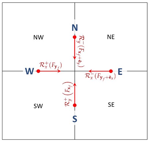
$Top view of the intersection between four neighbour zones in the $xy$ plane. N, S, E, and W indicate the four cardinal directions with respect to the zone edge (here represented by the intersection between four neighbour zones), $\mathcal {R}_x(F_{ {\boldsymbol {y}_{\rm f}} })$ and $\mathcal {R}_y(F_{ {\boldsymbol {x}_{\rm f}} })$ are 1D reconstruction operators applied to each zone face, see equations (49) and (51).$

Figure 1.

Top view of the intersection between four neighbour zones in the |$xy$| plane. N, S, E, and W indicate the four cardinal directions with respect to the zone edge (here represented by the intersection between four neighbour zones), |$\mathcal {R}_x(F_{ {\boldsymbol {y}_{\rm f}} })$| and |$\mathcal {R}_y(F_{ {\boldsymbol {x}_{\rm f}} })$| are 1D reconstruction operators applied to each zone face, see equations (49) and (51).

Open in new tab Download slide

Next, we also reconstruct the face-centred point values of the normal components of the magnetic field towards the same edge:

$$\begin{eqnarray} \begin{array}{l}B^S_{x, {\boldsymbol{z}_{\rm e}} } = {\cal R}^+_y(B_{x, {\boldsymbol {x}_{\rm f}} }) , \quad B^N_{x, {\boldsymbol{z}_{\rm e}} } = {\cal R}^-_y(B_{x, {\boldsymbol {x}_{\rm f}} +\hat{\boldsymbol {e}}_y}) , \\B^W_{y, {\boldsymbol{z}_{\rm e}} } = {\cal R}^+_y(B_{y, {\boldsymbol {y}_{\rm f}} }) , \quad B^E_{y, {\boldsymbol{z}_{\rm e}} } = {\cal R}^-_y(B_{y, {\boldsymbol {y}_{\rm f}} +\hat{\boldsymbol {e}}_x}). \end{array} \end{eqnarray}$$

(51)

Equations (49) and (51) allow us to obtain the edge-centred point value of the upwind electric field, using the CT-Maxwell averaging scheme (see section 3.4.2 of Paper I):

$$\begin{eqnarray} E_{z, {\boldsymbol{z}_{\rm e}} } = \left[\frac{E^N_z + E^S_z + E^W_z + E^E_z}{4} + \frac{B^E_{y}-B^W_{y}}{2}-\frac{B^N_{x}-B^S_{y}}{2}\right]_ {\boldsymbol{z}_{\rm e}}. \end{eqnarray}$$

(52)

Similar expressions hold for |$E_{x, {\boldsymbol{x}_{\rm e}} }$| and |$E_{y, {\boldsymbol{y}_{\rm e}} }$| by suitable index permutation.

Finally, we obtain the emf (i.e. the averaged line integral of the electric field needed in the discrete version of Faraday’s law equation 20) as

$$\begin{eqnarray} \bar{E}_{z, {\boldsymbol{z}_{\rm e}} } = \left(1 + \frac{\Delta ^z}{24}\right)E_{z, {\boldsymbol{z}_{\rm e}} } . \end{eqnarray}$$

(53)

Equations (51)–(53) are extended to the 3D case by suitable index permutation.

3.8 Explicit source term computation

In addition to the flux difference operator, the right-hand side (equation 18) requires an explicit contribution from the |$q\boldsymbol {v}$| source term during the electric field update. To fourth order, this term should be included as a volume average over the zone, i.e.

$$\begin{eqnarray} \left\langle {S} \right\rangle _{\rm e} = \left(1 + \frac{\Delta }{24}\right)q_ {\boldsymbol{c}} \boldsymbol {v}_ {\boldsymbol{c}} , \end{eqnarray}$$

(54)

where |$q_ {\boldsymbol{c}}$| and |$\boldsymbol {v}_ {\boldsymbol{c}}$| are, respectively, the point values of the charge and the fluid velocity. The former can be obtained from a cell-centred discretization of |$\nabla \cdot \boldsymbol {E}$| yielding

$$\begin{eqnarray} q_ {\boldsymbol{c}} = \delta _xE_x + \delta _yE_y + \delta _zE_z . \end{eqnarray}$$

(55)

Using the point value of the electric field already at disposal during the explicit step, we approximate (to fourth order) the x-contribution to the divergence as

$$\begin{eqnarray} \delta _x E_x = \frac{ 8\left(E_{x, {\boldsymbol{c}} +\hat{\boldsymbol {e}}_x}-E_{x, {\boldsymbol{c}} -\hat{\boldsymbol {e}}_x} \right)-\left(E_{x, {\boldsymbol{c}} +2\hat{\boldsymbol {e}}_x}-E_{x, {\boldsymbol{c}} -2\hat{\boldsymbol {e}}_x}\right)}{12\Delta x} . \end{eqnarray}$$

(56)

Contributions along the y- and z-directions are obtained in a similar way.

We point out that the employment of unlimited differences in equation (56) may lead to the appearance of spurious oscillations in the presence of strong gradients. This does not represent an issue for the tests presented below, but it could be further improved by including information from the reconstructed interface values (limited). We leave this investigation to a forthcoming work.

3.9 Order reduction at discontinuities

As pointed out in Paper II, fourth-order accuracy cannot be maintained in proximity of discontinuous solutions or steep gradients where the function may not be differentiable. In order to detect such features we compute, at the beginning of the RK step, the derivative ratio sensor as outlined in section 3.4 of Paper II. The detector flags computational cells where the order of the scheme can be locally reduced (this strategy is also known as ‘fallback’ process) by (i) not using the Laplacian during point value recovery and flux integration (equations 25 and 48) and (ii) switching to either third-order WENO or second-order linear reconstruction.

The detector employs a five-zone stencil and does not require additional ghost zones. A similar approach is also followed by Verma et al. (2019), albeit the authors make use of ‘global smoothness indicators’, defined in terms of weighted averages computed from the density and the three magnetic field components.

3.10 Algorithm summary

To better outline our algorithm, let |${\cal D}$| be the set of zones comprising the active computational domain (e.g. no ghost zones). Then |${\cal D}+1$| denotes the set of active computational zones augmented by one layer of ghost zones. Since the last step of an IMEX RK scheme is always explicit, our implementation can be best summarized starting from the end of the explicit stage |$(k*)$| (first part of equation 24) and moving on to the next, |$k\rightarrow (k+1)*$|⁠:

Start with the volume average of conservative variable, |$\left\langle {U} \right\rangle ^{(k*)}_ {\boldsymbol{c}}$|⁠, defined on |${\cal D}$| at the end of the more recent explicit stage.
Assign boundary conditions on |$\left\langle {U} \right\rangle _ {\boldsymbol{c}}$| in the first layer of ghost zones only so that |$\left\langle {U} \right\rangle _ {\boldsymbol{c}}$| is correctly specified on |${\cal D}+1$|⁠.
Recover the point value of conservative (⁠|$U_ {\boldsymbol{c}}$|⁠) and primitive variables, |$V_ {\boldsymbol{c}} = {\mathcal {V}}(U_ {\boldsymbol{c}})$| (as shown in Section 3.3), on |${\cal D}$| only.
Assign boundary conditions on |$V_ {\boldsymbol{c}}$|⁠. This will define primitive variables on |${\cal D}+n_g$|⁠, where |$n_g = 3$|⁠.
Carry out the implcit step by updating |$V_ {\boldsymbol{c}}$| on |${\cal D}+n_g$| as outlined in Section 3.4. Notice that conservative variables |$U_ {\boldsymbol{c}}$| do not change during this step, except for the electric field components.
Using the point value of primitive variables, compute the implicit source term point value in |${\cal D}+1$|⁠, i.e. |$S_ {\boldsymbol{c}} = S(V_ {\boldsymbol{c}})$|⁠.
Compute the zone-averaged implicit source term |$\left\langle {S} \right\rangle _ {\boldsymbol{c}}$| on |${\cal D}$| using Simpson quadrature rule.
Achieve the explicit step by constructing the right-hand side |$\hat{R}_ {\boldsymbol{c}}$| (equation 18) and its staggered version (right-hand side of equation 20):
- perform spatial reconstruction on primitive point value variables (Section 3.5);
- solve a Riemann problems with L/R states at zone interfaces, see Section 3.6;
- compute the surface-averaged flux using equation (48);
- compute the point value of the electric field at zone edges (equation 52) following the procedure outlined in Section 3.7;
- obtain the line-averaged emf through equation (53);
- compute the volume average of the explicit source term (Section 3.8).
Complete the explicit step by obtaining the volume-average conserved variables at the next RK stage, i.e. |$\left\langle {U} \right\rangle _ {\boldsymbol{c}} ^{(k+1)*}$|⁠.

Note that our formulation requires two boundary calls per stage: the first one is operated on |$\left\langle {U} \right\rangle _ {\boldsymbol{c}}$| but it extends only to one layer of ghost zones, while the second one specifies boundary values on the point value or primitive variables |$V_ {\boldsymbol{c}}$| and it extends to three ghost zones. Unlike previous works, our formulation does not require more than three ghost zones.

4 NUMERICAL BENCHMARKS

We now verify and assess the accuracy and robustness of our implementation through standard 2D and 3D reference solutions. Unless otherwise stated, we will employ the pointwise WENO-Z reconstruction (Paper II) and the MHLLC Riemann solver coupled with the CT-Maxwell emf average in all test problems. By default, order reduction (see Section 3.9) is disabled unless otherwise stated.

Initial conditions are integrated with a four-point Gaussian quadrature rule whenever smooth analytic functions are considered.

For quantitative purposes, we evaluate |$L_1$| norm errors for a generic quantity Q against a reference solution |$Q_{\rm ref}$| as |$\epsilon _1(Q) = \sum _i|Q(x_i)-Q_{\rm ref}(x_i)|/N$|⁠, where |$x_i$| is a generic point of the domain and N is the total number of grid zones.

All computations have been carried out by means of the pluto astrophysical code (Mignone et al. 2007, 2012), where the fourth-order resistive method has been implemented. The Courant number is set to 0.4 (in 2D) and 0.3 for 3D calculations.

4.1 Telegraph equation

In the fluid rest frame, the Res-RMHD equations can be employed to study the propagation of light waves in the presence of a finite conductivity, as originally presented in Mignone, Mattia & Bodo (2018) and Paper I. For a large plasma inertia (⁠|$\rho \rightarrow \infty$|⁠), only the Maxwell equations may be evolved in time:

$$\begin{eqnarray} \left\lbrace \begin{array}{l}\displaystyle \frac{\partial \boldsymbol {B}}{\partial t} + \nabla \times \boldsymbol {E} = 0, \\\displaystyle \frac{\partial \boldsymbol {E}}{\partial t} -\nabla \times \boldsymbol {B} = -\sigma \boldsymbol {E} . \end{array}\right. \end{eqnarray}$$

(57)

Equation (57) admits damped propagating plane wave solutions when |$\sigma \lt 2|k|$|⁠, where k is the wavenumber. The exact mode in one dimension is

$$\begin{eqnarray} \boldsymbol {B} &=&\displaystyle B_1 \, \mathrm{ e}^{-\sigma t/2}\cos \phi (x,t) \hat{\boldsymbol {n}}, \\\boldsymbol {E} &=&\displaystyle B_1 \, \mathrm{ e}^{-\sigma t/2} \left[\frac{\mu }{k} \cos \phi (x,t) +\frac{\sigma }{2k} \sin \phi (x,t)\right] \hat{\boldsymbol {n}}\times \hat{\boldsymbol {e}}_x , \end{eqnarray}$$

(58)

where |$\phi (x,t) = kx-\mu t$|⁠, |$\mu = (k^2-\sigma ^2/4)^{{1}/{2}}$|⁠, while |$B_1$| is the initial perturbation amplitude. Here, in addition to Paper I, we have introduced |$\hat{\boldsymbol {n}} = (0,\, \cos \Theta ,\, \sin \Theta)$| as the oscillation direction of the magnetic field in the |$yz$| plane.

Following Paper I, we rotate the 1D solution by an angle |$\alpha$| around the z-axis and consider the 2D computational domain |$x^{\prime }\in [0,L_x]$|⁠, |$y^{\prime }\in [0,L_y]$| with |$L_x=1$|⁠, |$L_y=1/2$| discretized with |$N_x\times N_x/2$| zones. Solving in a 2D domain allows us to assess the correct discretization of multidimensional terms. Electric and magnetic field vectors in this frame (⁠|$\boldsymbol {E}^{\prime }$| and |$\boldsymbol {B}^{\prime }$|⁠) are obtained through the rotation matrix

$$\begin{eqnarray} \lbrace \boldsymbol {E},\boldsymbol {B}\rbrace ^{\prime } = \begin{pmatrix}\cos \alpha & -\sin \alpha & 0 \\\sin \alpha & \cos \alpha & 0 \\0 & 0 & 1 \end{pmatrix}\lbrace \boldsymbol {E},\boldsymbol {B}\rbrace . \end{eqnarray}$$

(59)

The wave vector has orientation |$\boldsymbol {k}= k_x(1,\tan \alpha ,0)$|⁠, where |$k_x=2\pi /L_x$| while |$\tan \alpha = L_x/L_y = 2$|⁠. Equation (58) with |$B_1=1$| and |$\phi (\boldsymbol {x}^{\prime },0)=\boldsymbol {k}\cdot \boldsymbol {x}^{\prime }$| is used to initialize the electric and magnetic field. We also set density to a very large value (⁠|$\rho =10^{12}$|⁠), while velocity are set to zero. Periodic boundary conditions are imposed everywhere.

We employ the fourth-order ARK4 IMEX scheme and run computations at different grid resolutions for exactly one wave period |$T=2\pi /\mu$|⁠, where μ is defined after equation (58). In Fig. 2, we plot, from left to right, the profiles of |$B^{\prime }_z$| (at the resolution |$N_x=32$|⁠), the |$L_1$|-norm errors of |$\boldsymbol {B}\cdot \hat{\boldsymbol {n}}$| and |$\boldsymbol {E}\cdot (\hat{\boldsymbol {n}}\times \hat{\boldsymbol {e}}_x)$| as a function of the grid resolution (vectors are transformed back to the 1D frame), for |$\theta = 30^\circ$| (top panels) and |$\theta = 90^\circ$| (bottom panels). Green, blue, and red colours refer to computations obtained with |$\sigma = 1, \ 10$|⁠, and 20, respectively. In all cases, we recover the expected order of accuracy (4).

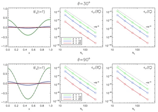
$Numerical results of the telegraph equation test, for $\theta = 30^\circ$ (top panels) and $\theta = 90^\circ$ (bottom panels). Left column: 1D horizontal profiles of $B^{\prime }_z$ using different values of the $\sigma = 1$, 10, and 20 for $N_x=32$. Central and right columns: L1 norm errors of $B^{*} = \boldsymbol {B}\cdot \hat{\boldsymbol {n}}$ and $E^{*}=\boldsymbol {E}\cdot (\hat{\boldsymbol {n}}\times \hat{\boldsymbol {e}}_x)$ as functions of the resolution. The dashed lines give the ideal convergence slope for the fourth order.$

Figure 2.

Numerical results of the telegraph equation test, for |$\theta = 30^\circ$| (top panels) and |$\theta = 90^\circ$| (bottom panels). Left column: 1D horizontal profiles of |$B^{\prime }_z$| using different values of the |$\sigma = 1$|⁠, 10, and 20 for |$N_x=32$|⁠. Central and right columns: L1 norm errors of |$B^{*} = \boldsymbol {B}\cdot \hat{\boldsymbol {n}}$| and |$E^{*}=\boldsymbol {E}\cdot (\hat{\boldsymbol {n}}\times \hat{\boldsymbol {e}}_x)$| as functions of the resolution. The dashed lines give the ideal convergence slope for the fourth order.

Open in new tab Download slide

4.2 Stationary charged vortex

We now consider an exact equilibrium solution of the full Res-RMHD equations, originally introduced in Paper I. It consists of a rotating charged flow embedded in a vertical magnetic field. Assuming purely radial dependence, hydrodynamic and electromagnetic variables are best expressed in a cylindrical coordinate system (⁠|$r,\, \phi ,\, z$|⁠) as

$$\begin{eqnarray} \left\lbrace \begin{array}{l}E_r = \displaystyle \frac{q_0}{2}\frac{r}{r^2+1}, \\B_z = \displaystyle \frac{\sqrt{(r^2 + 1)^2-q_0^2/4}}{r^2 + 1}, \\v_{\phi } = \displaystyle -\frac{q_0}{2}\frac{r}{\sqrt{(r^2+1)^2-q_0^2/4}}, \\p = -\displaystyle \frac{\rho }{\Gamma _1} + \left[ \frac{4r^2 + 4-q_0^2}{(r^2 + 1)(4-q_0^2)}\right]^{\Gamma _1/2} \left(p_0 + \displaystyle \frac{\rho }{\Gamma _1}\right), \\q = \displaystyle \frac{q_0}{(r^2+1)^2} , \end{array}\right. \end{eqnarray}$$

(60)

where |$\Gamma _1 = \Gamma /(\Gamma -1)$|⁠, |$p_0=0.1$|⁠, |$q_0=0.7$| is the charge at |$r=0$|⁠. Density is set to unity. The initial equilibrium condition given by equation (60) is mapped to a 2D Cartesian domain (⁠|$x,y\in [-10,10]$|⁠), and the system is evolved until |$t=5$|⁠. Boundary conditions replicate the equilibrium solution throughout the integration. Since the equilibrium condition does not depend on the resistivity, numerical computations with different values of the resistivity |$\eta$| depend solely on the stability of the algorithm.

For the present purpose, we have tested both the third-order SSP3(4,3,3) RK IMEX and the fourth-order ARK4 schemes. Results are shown in the four panels of Fig. 3. The integrity of the solution is effectively maintained. This is demonstrated by both the pressure colour map (top left panel) showing also isocontour levels of the electric field magnitude) and the 1D horizontal cuts of the charge (top right).

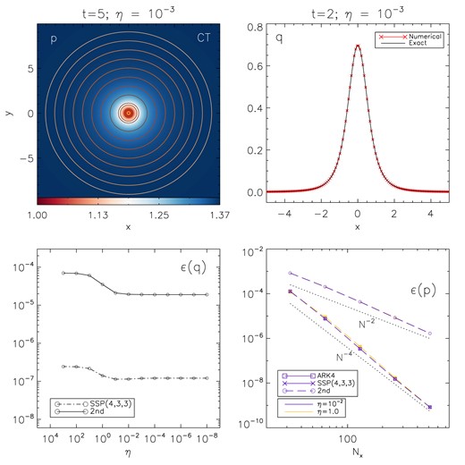
$Numerical results of the charged vortex problem. Top-left panel: We show eight equally spaced contour levels of E chosen as $(q_0 /2)r_k /(r_k^2 + 1)$ (where $r_k = 1, \ldots , 8$) overlaid on the coloured maps of pressure at $t = 5$. Resistivity is set to $\eta = 10^{-3}$ and the grid resolution is $256^2$ zones. Top-right panel: 1D horizontal cuts, at $y = 0$, of charge at $t = 3$ obtained with CT. Bottom-left panel: $L_1$ norm errors of the charge as functions of the resistivity using CT with $256^2$ zones. Bottom-right panel: $L_1$ norm errors of the gas pressure as functions of the resolution for the SSP(4,3,3), ARK4, and the second-order scheme. The dotted lines give the expected second-order scaling.$

Figure 3.

Numerical results of the charged vortex problem. Top-left panel: We show eight equally spaced contour levels of E chosen as |$(q_0 /2)r_k /(r_k^2 + 1)$| (where |$r_k = 1, \ldots , 8$|⁠) overlaid on the coloured maps of pressure at |$t = 5$|⁠. Resistivity is set to |$\eta = 10^{-3}$| and the grid resolution is |$256^2$| zones. Top-right panel: 1D horizontal cuts, at |$y = 0$|⁠, of charge at |$t = 3$| obtained with CT. Bottom-left panel: |$L_1$| norm errors of the charge as functions of the resistivity using CT with |$256^2$| zones. Bottom-right panel: |$L_1$| norm errors of the gas pressure as functions of the resolution for the SSP(4,3,3), ARK4, and the second-order scheme. The dotted lines give the expected second-order scaling.

Open in new tab Download slide

In the bottom left panel of Fig. 3, we plot the charge error as a function of the resistivity and compare our results with those of Paper I using a second-order method. Our fourth-order scheme is able to reduce the error by two orders of magnitude and we have found that both the SSP(4,3,3) and the ARK4 yield nearly identical results. However, the ARK4 method becomes unstable for |$\eta \lesssim 10^{-4}$|⁠. For this reason, we plot only the results obtained with the SSP method. Overall, the charge error exhibits minimal variation over time, underscoring the stability of the algorithm for any value of the resistivity parameter in the chosen range.

In the lower right quadrant of Fig. 3, we present the L1 norm errors of gas pressure against resolution, showcasing the achievement of fourth-order accuracy for both methods. Notably, in comparison with the results presented in Paper I, both charge and pressure errors are markedly reduced, with a two-order improvement in convergence.

4.3 2D relativistic rotor

We propose a resistive variant of the ideal special relativistic MHD test proposed by Del Zanna, Bucciantini & Londrillo (2003), as also presented by Dumbser & Zanotti (2009), Bucciantini & Del Zanna (2013), Miranda-Aranguren et al. (2018), and Nakamura et al. (2023). An overdense clump (⁠|$\rho = 10$|⁠) concentrated in a circular region (⁠|$r = 0.1$|⁠) at the centre of the computational square |$[-0.5, 0.5]^2$| is rapidly spinning (⁠|$\omega = 8.5$|⁠) in a uniform medium (⁠|$\rho = 1$|⁠, |$p = 1$|⁠, |$\Gamma = 4/3$|⁠) at rest. The vortex is embedded in a constant magnetic field |$\boldsymbol {B} = (1, 0, 0)$|⁠, which is progressively wrapping around the spinning vortex, launching torsional Alfvén waves in the ambient fluid. At the final time (⁠|$t = 0.3$|⁠), the torsional Alfvén waves have approximately been rotated at a |$90 {}^{\circ }$| angle, with the magnetic pressure deforming the initially circular vortex into its characteristic oval shape.

We perform a set of |$400 \times 400$| grid points simulations with increasing resistivity, from a quasi-ideal regime (⁠|$\eta = 10^{-6}$| and |$10^{-3}$|⁠) to a fully resistive one (⁠|$\eta = 10^{-1}$|⁠). Both the SSP(4,3,3) and the ARK4 were used for this test using order reduction to WENO3. As the resistivity increases, the vortex angular momentum as well as the torsional Alfvén waves that cause the well-known deformation are dissipated, leading to a more circular shape. Fig. 4 presents the snapshots of thermal pressure p (top panels) and the electric field |$E_z$| (bottom panels) at the final time |$t=0.3$|⁠. While results for SSP(4,3,3) appear essentially identical to those obtained with ARK4, only the former is able to successfully complete the integration with |$\eta = 10^{-6}$|⁠, again confirming the reduced stability of the fourth-order method, which is not SSP.

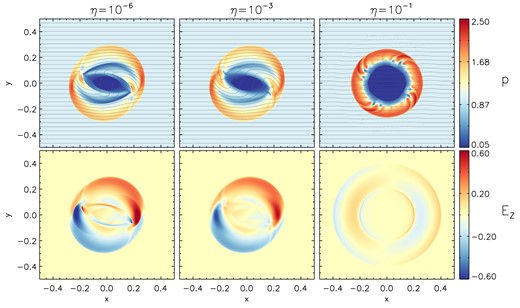
$Snapshots of the gas pressure p (upper panels) and profiles of $E_z$ (lower panels) for the resistive rotor test at its final time $t = 0.3$ at $400 \times 400$ grid points using the SSP3(4,3,3) IMEX time-stepping. From left to right, results correspond to computations with different resistivities $\eta = 10^{-6}$, $\eta = 10^{-3}$, and $\eta = 10^{-1}$.$

Figure 4.

Snapshots of the gas pressure p (upper panels) and profiles of |$E_z$| (lower panels) for the resistive rotor test at its final time |$t = 0.3$| at |$400 \times 400$| grid points using the SSP3(4,3,3) IMEX time-stepping. From left to right, results correspond to computations with different resistivities |$\eta = 10^{-6}$|⁠, |$\eta = 10^{-3}$|⁠, and |$\eta = 10^{-1}$|⁠.

Open in new tab Download slide

It is relevant to notice how the pressure distribution is affected by the onset of spurious modes (⁠|$m=4$|⁠) in the most resistive regime (⁠|$\eta = 10^{-1}$|⁠). This artefact results from the employment of Cartesian coordinates and it becomes more evident when using a MHLLC solver rather than a more diffusive one (with which the effect is substantially mitigated).

4.4 3D blast wave

The magnetized blast wave problem is used here to assess the robustness of the numerical method in handling the propagation of shock waves through magnetic field of varying strength as well as the capacity of preserving the symmetric properties of the solution. In fact, unphysical features could emerge if the divergence-free condition is not properly controlled (see e.g. Mignone & Bodo 2006; Del Zanna et al. 2007).

Following Paper I, we consider the computational domain |$x,y,z\in [-6,6]$| threaded by a uniform magnetic field |$\boldsymbol {B}= B_0\hat{\boldsymbol {e}}_x$| with |$B_0=0.1$|⁠. The plasma is initially at rest while density and pressure experience a sharp transition across a sphere of radius |$r_c=0.8$|⁠:

$$\begin{eqnarray} \begin{pmatrix}\rho \\p \end{pmatrix} = f_\mathrm{ t}(r)\begin{pmatrix}\rho _{\rm in} \\p_{\rm in} \end{pmatrix} + \left(1 \cdots f_\mathrm{ t}(r)\right) \begin{pmatrix}\rho _{\rm out} \\p_{\rm out} \end{pmatrix}, \end{eqnarray}$$

(61)

where |$f_\mathrm{ t}(r)$| is a taper (smoothing) function,

$$\begin{eqnarray} f_\mathrm{ t}(r) = \max \left[\min \left(\frac{e^\chi -e}{1-e},1\right),0\right] , \end{eqnarray}$$

(62)

with |$\chi = (r-r_c)/(1-r_c)$|⁠. Similar 3D configurations have been used by Komissarov (2007) and Dionysopoulou et al. (2013), although with larger resistivity or lower magnetic fields. The system is evolved until |$t=4$| using the SSP(4,3,3) method. We also enable order reduction to be linear for this test. Zero-gradient boundary conditions apply everywhere.

Fig. 5 shows the outcomes of the simulation, presenting, in the top panel, 2D maps of the x-component of magnetic field (left), gas pressure (middle) while, in the bottom panel, electromagnetic pressure (left) and Lorentz factor (middle). In the rightmost column, we show one-dimensional profiles along the z-axis of thermal pressure (top) and Lorentz factor (bottom). As a consequence of the explosion, a swiftly advancing forward shock moves in an (almost) radial manner, while concurrently, a trailing reverse shock marks the boundary of the internal region where radial expansion occurs. Electromagnetic fields pile up in the y-direction, forming a shell characterized by elevated magnetic pressure. Gas exhibits a pronounced preference for motion along the x-direction, attaining a heightened Lorentz factor (⁠|$\gamma _{\max } \approx 5.4$|⁠).

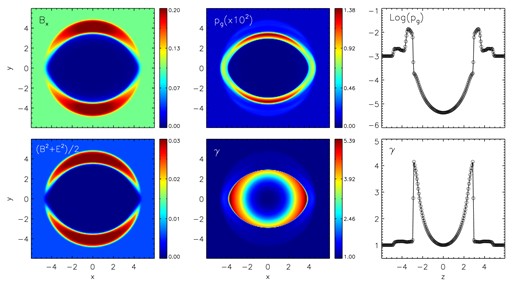
$3D blast wave at $t = 4$ using $\eta = 10^{-6}$ and the CT scheme. In the top panels, we show 2D slices in the $xy$ plane of $B_x$ (left), gas pressure $p_\mathrm{ g}$ (middle), and its 1D profile along the z-axis (right). In the bottom panels, we show 2D slices of the electromagnetic pressure (left), Lorentz factor (middle), and its cuts along the z-axis (right).$

Figure 5.

3D blast wave at |$t = 4$| using |$\eta = 10^{-6}$| and the CT scheme. In the top panels, we show 2D slices in the |$xy$| plane of |$B_x$| (left), gas pressure |$p_\mathrm{ g}$| (middle), and its 1D profile along the z-axis (right). In the bottom panels, we show 2D slices of the electromagnetic pressure (left), Lorentz factor (middle), and its cuts along the z-axis (right).

Open in new tab Download slide

4.5 Tearing mode

In what follows we validate our method on the linear growth of the ideal tearing mode instability with a Harris current sheet profile, following the results presented by Del Zanna et al. (2016, see also Miranda-Aranguren et al. 2018; Paper I).

In this problem, a static (⁠|$v = 0$|⁠) plasma is uniformly distributed in the computational domain with constant initial density and pressure |$\rho _0$| and |$p_0$|⁠. The initial magnetic field profile satisfies the force-free condition and it is given by

$$\begin{eqnarray} {\boldsymbol B} = B_0 \left[\tanh \left(\frac{x}{a} \right) \hat{\boldsymbol {e}}_y + \operatorname{sech}~\left(\frac{x}{a} \right) \hat{\boldsymbol {e}}_z \right] , \end{eqnarray}$$

(63)

while the initial electric field is null everywhere. The physical parameters that set the proper conditions for the instability to grow are the current sheet thickness a, the magnetization |$\Sigma = B_0^2/\rho _0$|⁠, the plasma beta |$\beta = 2p_0 /B_0^2$|⁠, the Alfvén velocity |$v_\mathrm{ a} = B_0 /\sqrt{B_0^2 + w_0} = B_0 /\sqrt{B_0^2 + \rho _0 + 4p_0}$| obtained by assuming an ideal gas law with relativistic adiabatic index |$\Gamma = 4/3$|⁠, and the Lundquist number |$S = v_\mathrm{ a} L/\eta$|⁠, where |$\eta$| is the resistivity and L is the reference spatial scale of variation. In order to trigger the instability, |$S\gg 1$|⁠.

Generalizing the MHD results obtained by Pucci & Velli (2014) and Landi et al. (2015) to this regime, provided a sufficiently thin current sheet, the reconnection process is expected to occur on the ideal Alfvénic time-scale |$\tau _\mathrm{ a} = L/v_\mathrm{ a}$|⁠. The critical (inverse) aspect ratio determining this regime is

$$\begin{eqnarray} a = S^{-1/3} L . \end{eqnarray}$$

(64)

In the limit of large S, the growth rate |$\gamma _{\rm TM}$| of the instability becomes |$\gamma _{\rm TM} \simeq 0.6 v_{\rm a}/L$|⁠, which, in a relativistic regime (⁠|$v_\mathrm{ a} \rightarrow c = 1$|⁠), results in a very efficient process commonly referred to as ideal tearing instability.

The initial equilibrium is perturbed by a small amplitude (⁠|$\epsilon = 10^{-4}$|⁠) variation in the magnetic field employing only one wavenumber k:

$$\begin{eqnarray} \displaystyle \delta {\boldsymbol B} = \epsilon B_0 \operatorname{sech}~\left(\frac{x}{a} \right) \begin{pmatrix}\displaystyle \cos (ky) \\\displaystyle \frac{\sin (ky)}{ka} \tanh \left(\frac{x}{a} \right) \\\displaystyle 0 \end{pmatrix} . \end{eqnarray}$$

(65)

Following section 5.5 of Paper I, we initialize the magnetic field in the |$xy$| plane with the vector potential

$$\begin{eqnarray} \displaystyle A_z = -B_0 \left[a \log \left(\cosh \frac{x}{a} \right)-\frac{\epsilon }{k} \sin (ky)\operatorname{sech}\left(\frac{x}{a} \right) \right] . \end{eqnarray}$$

(66)

In accordance with the work developed by Del Zanna et al. (2016) and later resumed in Paper I, the linear theory predicts that the wavenumber associated with the fastest growing mode of the ideal tearing instability is |$k_{\rm max} = 1.4 S^{1/6} = 14$|⁠. The corresponding growth rate is |$\gamma _{\rm TM} \simeq 0.3$|⁠. None the less, due to the neglection of the compressible terms in the linear approximation as presented in Del Zanna et al. (2016), the maximum value of the dispersion relation is shifted to |$k = 12$| with the consequent modification of the expected growth rate to |$\gamma _{\rm TM} \simeq 0.27$|⁠. We therefore align with the works of Del Zanna et al. (2016), Miranda-Aranguren et al. (2018), and Paper I and choose |$k = 12$| for our simulations. Likewise, we set |$L = B_0 = \Sigma = \beta = 1$|⁠, deriving therefore |$\rho _0 = 1$|⁠, |$p_0 = 0.5$|⁠, |$v_\mathrm{ a} = 0.5$|⁠, and |$S = 10^6$|⁠. In this way |$a = 0.01$| and |$\eta = 5 \times 10^{-7}$|⁠. In order to recover the predicted growth rate, we perform a set of simulations with increasing resolution |$N_x \times N_x/4$| (⁠|$N_x = \lbrace 256, 512, 1024, 2048\rbrace$|⁠), on a rectangular computational domain with |$x \in [-20a, 20a] = [-0.2, 0.2]$| and outflow boundary conditions, and |$y \in [0, 0.523598]$| imposing periodicity along y. Simulations have been carried out until |$t = 20$| using the IMEX SSP(4,3,3) time-stepping.

In the left and middle panels of Fig. 6, we plot the horizontal cuts at |$y=0$| of the x-components of the magnetic field (left panel), velocity (middle panel) at |$t=10$| for all resolutions. The magnetic field at all resolutions closely resembles the eigenfunction solutions presented by Del Zanna et al. (2016) (see fig. 1 of that paper). The same holds for the velocity profile, although a more pronounced dependency on resolution is observed along with some clipping. Following Miranda-Aranguren et al. (2018) and Paper I, we measure the growth rate by first computing

$$\begin{eqnarray} \gamma (t) = \displaystyle \frac{1}{2}\log \left(\int B^2_x(t) \, \mathrm{ d}S \right) , \end{eqnarray}$$

(67)

which we plot, as a function of time, in the right panel of Fig. 6 (solid lines) along with the second-order data from Paper I (dotted lines) for each resolution. The growth rate is then computed from a linear fit of equation (67), while the red dashed–dotted line represents the ideal value (⁠|$\gamma _{\rm TM} \simeq 0.27$|⁠). Table 1 compares the results obtained with the second- and fourth-order scheme (middle and right columns, respectively). For each slope, a different time window has been chosen in order to properly fit the linear growth of the fastest growing mode (crosses in Fig. 6) during the first linear phase. While both the second- and fourth-order schemes show systematic convergence towards the predicted value, the latter requires approximately half of the resolution (or less) to reproduce the results of the former. The best agreement is reached with the fourth-order scheme using 2048 zones.

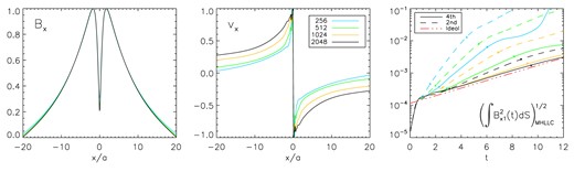
$Horizontal cuts of the x-component of the magnetic field (left panel), and of the velocity (middle panel) for the tearing mode instability at $t = 10$. The profiles are normalized to unity and show the trends along $y = 0$ for the magnetic field (left panel), and along $({3}/{4})L_y$ for the velocity (middle panel). Each resolution ($N_x = \lbrace 256, 512, 1024, 2048\rbrace$) is demarked with a different colour. Measured growth rates (right panel) are plotted as solid (dashed) lines for the fourth-order (second-order) data and are compared to the ideal trend (dashed–dotted line). Crosses mark the time intervals for which each growth rate has been calculated.$

Figure 6.

Horizontal cuts of the x-component of the magnetic field (left panel), and of the velocity (middle panel) for the tearing mode instability at |$t = 10$|⁠. The profiles are normalized to unity and show the trends along |$y = 0$| for the magnetic field (left panel), and along |$({3}/{4})L_y$| for the velocity (middle panel). Each resolution (⁠|$N_x = \lbrace 256, 512, 1024, 2048\rbrace$|⁠) is demarked with a different colour. Measured growth rates (right panel) are plotted as solid (dashed) lines for the fourth-order (second-order) data and are compared to the ideal trend (dashed–dotted line). Crosses mark the time intervals for which each growth rate has been calculated.

Open in new tab Download slide

Table 1.

Open in new tab

Growth rates of the linear phase of the tearing instability as measured from the second- and fourth-order simulation data, listed by resolution. The measured growth rates refer to the onset of the first linear phase of the instability. The time intervals chosen to evaluate each slope are marked as crosses in the right panel of Fig. 6.

Resolution	Second order	Fourth order
\|$256\times 64$\|	1.19	0.75
\|$512\times 128$\|	0.89	0.44
\|$1024\times 256$\|	0.58	0.30
\|$2048\times 512$\|	0.38	0.27

Table 1.

Open in new tab

Resolution	Second order	Fourth order
\|$256\times 64$\|	1.19	0.75
\|$512\times 128$\|	0.89	0.44
\|$1024\times 256$\|	0.58	0.30
\|$2048\times 512$\|	0.38	0.27

4.6 3D Kelvin–Helmholtz instability

As a final application benchmark, we consider a 3D version of Kelvin–Helmholtz instability in relativistic MHD (see e.g. Bucciantini & Del Zanna 2006) as presented in Paper I and earlier, in 2D, also by Beckwith & Stone (2011) and Mizuno (2013). At |$t=0$|⁠, we prescribe a double shear layer configuration with non-uniform density and constant magnetic field:

$$\begin{eqnarray} \displaystyle \rho &=& \frac{1+\tanh \phi (y)}{2}\rho _{\rm h} + \frac{1-\tanh \phi (y)}{2}\rho _{\rm h} , \\\displaystyle \boldsymbol {v} &=& v_{\rm sh}\tanh \phi (y)\hat{\boldsymbol {e}}_x + A_0\left[{\rm sign}(y)\sin (2\pi x)\hat{\boldsymbol {e}}_y + \zeta \hat{\boldsymbol {e}}_z\right] f(y) , \\\displaystyle \boldsymbol {B}& = & \left(\sqrt{2p\sigma \mu _{\rm p}},\, 0,\, \sqrt{2p\sigma \mu _{\rm t}} \right), \end{eqnarray}$$

(68)

where |$v_{\rm sh} = 1/2$| is the shear velocity, |$a = 0.01$| is the shear thickness, |$\phi (y) = (|y|-1/2)/a$| while |$A_0=0.1$| is the perturbation amplitude, and |$\zeta$| is a random number in the range |$[-1,1]$|⁠. The function

$$\begin{eqnarray} f(y) = \mathrm{ e}^{-\phi ^2a^2/\alpha ^2} \end{eqnarray}$$

(69)

(with |$\alpha =0.1$|⁠) is used to dampen the perturbations as we move away from the two interfaces located at |$y=\pm 1/2$|⁠. The parameters |$\mu _{\rm p}$| and |$\mu _{\rm t}$| control the in plane (⁠|$\mu _{\rm p} = 0.01$|⁠) and out of plane (⁠|$\mu _{\rm t} = 1$|⁠) magnetic field strength. We set resistivity to |$\eta = 1/\sigma =10^{-5}$| and evolve the system until |$t=30$| using the MHLLC Riemann solver. Following Paper I, we perform simulations on the Cartesian domain |$x,z\in [-1/2,1/2]$| and |$y\in [-1,1]$| with uniform grid resolution |$N\times 2N\times N$|⁠, with |$N=128$| (low resolution) and |$N=256$| (high resolution).

Simulations have been repeated with both the high-order scheme – employing IMEX SSP3(4,3,3) time-stepping – as well as using also the second-order scheme presented in Paper I, based on piecewise linear reconstruction and the second-order IMEX time-stepping. For the fourth-order method, we employ order reduction (linear).

The time evolution of the instability can be observed in Fig. 7 where we show 2D slices at |$z=0$| for density (first and second row from top) and poloidal to toroidal magnetic field (third and fourth) with |$N=256$|⁠. The large-scale motion remains confined along the initial shear direction and the turbulent state is characterized by sheet-like thin structures, where most of the magnetic field energy is trapped. These rounded slabs remain roughly parallel to the |$xz$| plane, although significant medium-scale structures develop in this direction for |$t\gtrsim 20$| around the shear layer.

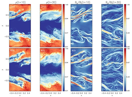
$2D slice cut of the density and poloidal to toroidal magnetic field at $z=0$ for the 3D Kelvin–Helmholtz instability at $t = 10$ and 30 at the resolution of $256\times 512\times 256$ zones. Here $B_{\rm p} = \sqrt{B_x^2 + B_y^2}$.$

Figure 7.

2D slice cut of the density and poloidal to toroidal magnetic field at |$z=0$| for the 3D Kelvin–Helmholtz instability at |$t = 10$| and 30 at the resolution of |$256\times 512\times 256$| zones. Here |$B_{\rm p} = \sqrt{B_x^2 + B_y^2}$|⁠.

Open in new tab Download slide

A direct measure of the growth rate, quantified by |$\Delta v_y = (\max (v_y)-\min (v_y))/2$|⁠, is shown in the top-left panel of Fig. 8 for both the second- and fourth-order simulations at low and high resolutions (blue and red colours, respectively). As noticed in Paper I (see fig. 11 of that paper), with the MHLLC Riemann solver, an increase in resolution (or scheme accuracy) is accompanied by a gradual reduction of the growth rate, until convergence is finally reached. This is also the case here and clearly visible with the second-order method (red lines) but only marginally with the fourth-order scheme that shows better convergence properties at low resolution. A quantitative measure of the growth rate, in the range given by the circle symbols in the figure, yields indeed |${\approx} 2.94$| and |${\approx} 2.14$| for the second-order scheme (low and high resolution, respectively) and |${\approx} 2.17$| and |${\approx} 2.31$| for the fourth-order scheme.

$Top panels: Growth rate (left) and volume-integrated electromagnetic $P_{\rm em} = (\boldsymbol {B}^2+\boldsymbol {E}^2)/2$ (middle) and kinetic $E_{\rm kin} = \rho \gamma (\gamma -1)$ (right) as a function of time for the 3D Kelvin–Helmholtz instability. Circles in the top-left plot mark the time windows used to compute the growth rate. Bottom panels: From left to right, spectral energy densities in the x-, y-, and z-direction at $t = 15$. Solid and dashed lines are used for the fourth- and second-order schemes, while different colors are used for the resolution of $128\times 256\times 128$ and $256\times 512\times 256$ zones, respectively.$

Figure 8.

Top panels: Growth rate (left) and volume-integrated electromagnetic |$P_{\rm em} = (\boldsymbol {B}^2+\boldsymbol {E}^2)/2$| (middle) and kinetic |$E_{\rm kin} = \rho \gamma (\gamma -1)$| (right) as a function of time for the 3D Kelvin–Helmholtz instability. Circles in the top-left plot mark the time windows used to compute the growth rate. Bottom panels: From left to right, spectral energy densities in the x-, y-, and z-direction at |$t = 15$|⁠. Solid and dashed lines are used for the fourth- and second-order schemes, while different colors are used for the resolution of |$128\times 256\times 128$| and |$256\times 512\times 256$| zones, respectively.

Open in new tab Download slide

The enhanced dissipation of electromagnetic and kinetic energies (top middle and right panels in Fig. 8) using our high-order scheme stems from the increased turbulence that comes from having an effective dissipation at scales smaller than the low-order case. In this sense, the performance of our high-order scheme at low resolutions (⁠|$N_x=128$|⁠) already outperforms the one obtained by the second-order scheme at twice the resolution.

The amount of small-scale features is an indirect measurement of the numerical dissipation, which we quantify through the spectral energy density,

$$\begin{eqnarray} P(k_x) = \int |{\cal F}(k_x,y,z)|^2 \, \mathrm{ d}y\, \mathrm{ d}z , \end{eqnarray}$$

(70)

where |${\cal F}(k_x,y,z)$| is the 1D fast Fourier transform of the density taken across the x dimension. |$P(k_y)$| and |$P(k_z)$| are constructed similarly, by corresponding index permutations. Results, shown in the bottom row of Fig. 8 (⁠|$P(k_y)$| and |$P(k_z)$|⁠), indicate that large-scale modes are better resolved with the fourth-order scheme.

5 SUMMARY

We have presented a genuinely fourth-order FV algorithm for the solution of the Res-RMHD equations in multiple dimensions. To our knowledge, this is one of the few contributions addressing the design of the fourth-order methods based on an IMEX approach for multidimensional PDEs with stiff terms.

High-order quadrature rules to obtain volume, surface, or line averages are evaluated using appropriate Simpson rules, as outlined in the seminal paper by McCorquodale & Colella (2011). Point values are recovered from volume (or surface) averages following the opposite procedure. The fourth-order spatial accuracy is achieved by reconstructing point values (rather than 1D volume averages) using the modified WENO-Z reconstruction of Paper II, while for temporal integration, we have implemented and compared the third-order RK IMEX SSP3(4,3,3) scheme of Pareschi & Russo (2003, 2005) with the fourth-order IMEX-ARK4(3)7L[2]SA_1 scheme of Kennedy & Carpenter (2019) (ARK). The divergence-free condition is ensured by evolving magnetic fields according to the CT formalism, while the electric field is treated as a volume average quantity. Equations are evolved in conservation form, requiring the solution of a Riemann problem between discontinuous left and right states at zone interfaces. Our scheme employs only three ghost zones, and thus a more compact stencil when compared to its previous version (Paper II).

Numerical benchmarks in two and three dimensions demonstrate the accuracy of the method along with reduced numerical dissipation. For smooth problems, our results show superior accuracy and faster convergence when compared to the standard second-order schemes. While the ARK4 retains the temporal fourth-order accuracy for smooth problems, we found in our experience that the third-order SSP scheme is more robust for lower values of the resistivity, |$\eta \lesssim 10^{-5}$|⁠, and thus preferable for highly stiff problems.

The scheme can also cope with complex flow features including steep gradients and discontinuous waves, although the spatial order of the scheme may have to be locally reduced (‘fallback’ approach) so as to enhance robustness in critical regions. To identify such regions, we employ the discontinuity detector proposed in Paper II, based on the ratio of derivative, specifically designed to detect high-frequency oscillations typically arising in proximity of a discontinuous front.

The employment of genuinely fourth-order methods may represent a major upgrade in the field of astrophysical plasma computations, allowing more accurate computations at a reduced cost.

ACKNOWLEDGEMENTS

Computational resources were provided by the Centro di Competenza sul Calcolo Scientifico (C3S) of the University of Torino (c3s.unito.it).

This project has received funding from the European Union’s Horizon Europe research and innovation programme under the Marie Skłodowska-Curie grant agreement no. 101064953 (GR-PLUTO).

This work has received funding from the European High Performance Computing Joint Undertaking (JU) and Belgium, Czech Republic, France, Germany, Greece, Italy, Norway, and Spain under grant agreement no. 101093441 (SPACE).

This paper was supported by the Fondazione ICSC, Spoke 3 Astrophysics and Cosmos Observations. National Recovery and Resilience Plan (Piano Nazionale di Ripresa e Resilienza, PNRR) Project ID CN_00000013 ‘Italian Research Center on High-Performance Computing, Big Data and Quantum Computing’ funded by MUR Missione 4 Componente 2 Investimento 1.4: Potenziamento strutture di ricerca e creazione di ‘campioni nazionali di |${\rm R\&S}$| (M4C2-19)’ – Next Generation EU (NGEU).

The partial support from Gruppo Nazionale Calcolo Scientifico-Istituto Nazionale di Alta Matematica (GNCS INdAM) and MIUR-PRIN Project 2022, no. 2022KKJP4X ‘Advanced numerical methods for time-dependent parametric partial differential equations with applications’ is also acknowledged.

DATA AVAILABILITY

The data underlying this article will be shared on reasonable request to the corresponding author.

Footnotes

The approach followed here differs from the one employed in Paper I, where the reconstruction is performed from the cell centre using linear interpolation. Also, a typo is present in equation (48) of Paper I, since the arithmetic average operator |$\left\langle {.} \right\rangle _z$| is not needed.

REFERENCES

Ascher

U. M.

Ruuth

S. J.

Spiteri

R. J.

1997

Appl. Numer. Math.

151

Month:	Total Views:
July 2024	8
August 2024	93
September 2024	179
October 2024	88
November 2024	41
December 2024	40
January 2025	49
February 2025	38
March 2025	36
April 2025	26
May 2025	21

Article Contents

A fourth-order accurate finite volume scheme for resistive relativistic MHD Open Access

ABSTRACT

1 INTRODUCTION

2 RESISTIVE RELATIVISTIC MHD EQUATIONS

3 NUMERICAL METHOD

3.1 Basic discretization

3.2 Temporal update

3.3 Point value recovery of primitive variables

3.4 Implicit update of pointwise quantities

3.5 Point value reconstruction of primitive variables

3.6 Riemann solver and flux computation

3.7 Constrained transport update

3.8 Explicit source term computation

3.9 Order reduction at discontinuities

3.10 Algorithm summary

4 NUMERICAL BENCHMARKS

4.1 Telegraph equation

4.2 Stationary charged vortex

4.3 2D relativistic rotor

4.4 3D blast wave

4.5 Tearing mode

4.6 3D Kelvin–Helmholtz instability

5 SUMMARY

ACKNOWLEDGEMENTS

DATA AVAILABILITY

Footnotes

REFERENCES

APPENDIX A: EXPLICIT BUTCHER TABLEAUX

Citations

Views

Altmetric

Email alerts

Astrophysics Data System

Citing articles via

Latest

Most Read

Most Cited

This Feature Is Available To Subscribers Only

A fourth-order accurate finite volume scheme for resistive relativistic MHD