


ABSTRACT
We use angular clustering of luminous red galaxies from the Dark Energy Spectroscopic Instrument (DESI) imaging surveys to constrain the local primordial non-Gaussianity parameter fNL. Our sample comprises over 12 million targets, covering 14 000 deg2 of the sky, with redshifts in the range 0.2 < z < 1.35. We identify Galactic extinction, survey depth, and astronomical seeing as the primary sources of systematic error, and employ linear regression and artificial neural networks to alleviate non-cosmological excess clustering on large scales. Our methods are tested against simulations with and without fNL and systematics, showing superior performance of the neural network treatment. The neural network with a set of nine imaging property maps passes our systematic null test criteria, and is chosen as the fiducial treatment. Assuming the universality relation, we find |$f_{\rm NL} = 34^{+24(+50)}_{-44(-73)}$| at 68 per cent (95 per cent) confidence. We apply a series of robustness tests (e.g. cuts on imaging, declination, or scales used) that show consistency in the obtained constraints. We study how the regression method biases the measured angular power spectrum and degrades the fNL constraining power. The use of the nine maps more than doubles the uncertainty compared to using only the three primary maps in the regression. Our results thus motivate the development of more efficient methods that avoid overcorrection, protect large-scale clustering information, and preserve constraining power. Additionally, our results encourage further studies of fNL with DESI spectroscopic samples, where the inclusion of 3D clustering modes should help separate imaging systematics and lessen the degradation in the fNL uncertainty.
1 INTRODUCTION
Inflation is a widely accepted paradigm in modern cosmology that explains many important characteristics of our Universe. It predicts that the early Universe underwent a period of accelerated expansion, resulting in the observed homogeneity and isotropy of the Universe on large scales (Guth 1981; Linde 1982; Albrecht & Steinhardt 1982). After the period of inflation, the Universe entered a phase of reheating in which primordial perturbations were generated, setting the initial seeds for structure formation (Kofman, Linde & Starobinsky 1994; Bassett, Tsujikawa & Wands 2006; Lyth & Liddle 2009). Although inflation is widely accepted as a compelling explanation, the characteristics of the field or fields that drove the inflationary expansion remain largely unknown in cosmology. While early studies of the cosmic microwave background (CMB) and large-scale structure (LSS) suggested that primordial fluctuations are both Gaussian and scale-invariant (Komatsu et al. 2003; Tegmark et al. 2004; Guth & Kaiser 2005), some alternative classes of inflationary models predict different levels of non-Gaussianities in the primordial gravitational field. Non-Gaussianities are a measure of the degree to which the distribution of matter in the Universe deviates from a Gaussian distribution, which would have important implications for the growth of structure and galaxies in the Universe (see e.g. Verde 2010; Desjacques & Seljak 2010; Biagetti2019).
In its simplest form, local primordial non-Gaussianity (PNG) is parametrized by the non-linear coupling constant fNL(Komatsu & Spergel 2001):
where Φ is the primordial curvature perturbation and ϕ is assumed to be a Gaussian random field. Local-type PNG generates a primordial bispectrum, which peaks in the squeezed triangle configuration where one of the three wave vectors is much smaller than the other two. This means that one of the modes is on a much larger scale than the other two, and this mode couples with the other two modes to generate a non-Gaussian signal, which then affects the local number density of galaxies. The coupling between the short and long wavelengths induces a distinct bias in the galaxy distribution, which leads to a k−2-dependent feature in the two-point clustering of galaxies and quasars (Dalal et al. 2008). Obtaining reliable, accurate, and robust constraints on fNL is crucial in advancing our understanding of the dynamics of the early Universe. For instance, the standard single-field slow-roll inflationary model predicts a small value of fNL ∼ 0.01 (see e.g. Maldacena 2003). On the other hand, some alternative inflationary scenarios involve multiple scalar fields that can interact with each other during inflation, leading to the generation of larger levels of non-Gaussianities. These models predict considerably larger values of fNL that can reach up to 100 or higher (see e.g. Chen 2010, for a review). With σ(fNL) ∼ 1, we can rule out or confirm specific models of inflation and gain insight into the physics that drove the inflationary expansion (see e.g. Alvarez et al. 2014; de Putter, Gleyzes & Doré 2017).
The current tightest bound on fNL comes from Planck’s bispectrum measurement of CMB anisotropies, fNL = 0.9 ± 5.1 (Planck Collaboration IX 2020). Limited by cosmic variance, CMB data cannot enhance the statistical precision of fNL measurements enough to break the degeneracy amongst various inflationary paradigms (see e.g. Abazajian et al. 2016; Simons Observatory et al. 2019). On the other hand, LSS surveys probe a 3D map of the Universe, and thus provide more modes to limit fNL. However, non-linearities raised from structure formation pose a serious challenge for measuring fNL with the three-point clustering of galaxies, and these non-linear effects are non-trivial to model and disentangle from the primordial signal (Baldauf et al. 2011b; Baldauf, Seljak & Senatore 2011a). Currently, the most precise constraints on fNL from LSS reach a level of σ(fNL) ∼ 20–30, with the majority of the constraining power coming from the two-point clustering statistics that utilize the scale-dependent bias effect (Slosar et al. 2008; Ross et al. 2013; Castorina et al. 2019; Mueller et al. 2022; Cabass et al. 2022; D’Amico et al. 2022). Surveying large areas of the sky can unlock more modes and help improve these constraints.
The Dark Energy Spectroscopic Instrument (DESI) is ideally suited to enable excellent constraints on PNG from the galaxy distribution. DESI uses 5000 robotically driven fibres to simultaneously collect spectra of extragalactic objects (Levi et al. 2013; DESI Collaboration 2016b; Silber et al. 2023). DESI is designed to deliver an unparalleled volume of spectroscopic data covering |$\sim 14\, 000$| deg2 that promises to deepen our understanding of the energy contents of the Universe, neutrino masses, and the nature of gravity (DESI Collaboration 2022). Moreover, DESI alone is expected to improve our constraints on local PNG down to σ(fNL) = 5, assuming systematic uncertainties are under control (DESI Collaboration 2016a). With multitracer techniques (Seljak 2009), cosmic variance can be further reduced to allow surpassing CMB-like constraints (Alonso et al. 2015). For instance, the distortion of CMB photons around foreground masses, which is referred to as CMB lensing, provides an additional probe of LSS, but from a different vantage point. We can significantly reduce statistical uncertainties below σ(fNL) ∼ 1 by cross-correlating LSS data with CMB-lensing, or other tracers of matter, such as 21 cm intensity mapping (see e.g. Schmittfull & Seljak 2018; Heinrich & Doré 2022; Jolicoeur, Maartens & Dlamini 2023; Sullivan, Prijon & Seljak 2023).
However, further work is needed to fully harness the potential of the scale-dependent bias effect in constraining fNL with LSS. The amplitude of the fNL signal in the galaxy distribution is proportional to the bias parameter bϕ, such that Δb ∝ bϕfNLk−2. Assuming the universality relation, bϕ ∼ (b − p), where b is the linear halo bias and p = 1 is a parameter that describes the response of galaxy formation to primordial potential perturbations in the presence of local PNG (see e.g. Slosar et al. 2008). The value of p is not very well constrained for other tracers of matter (Barreira et al. 2020; Barreira 2020), and Barreira (2022) showed that marginalizing over p even with wide priors leads to biased fNL constraints because of parameter space projection effects. More simulation-based studies are necessary to investigate the halo-assembly bias and the relationship between bϕ and b for various galaxy samples. For instance, Lazeyras et al. (2023) used N-body simulations to investigate secondary halo properties, such as concentration, spin, and sphericity of haloes, and found that halo spin and sphericity preserve the universality of the halo occupation function while halo concentration significantly alters the halo function. Without better-informed priors on p, it is argued that the scale-dependent bias effect can only be used to constrain the bϕfNL term (see e.g. Barreira 2020). However, regardless of the specific value of p, a non-zero detection of bϕfNL implies the presence of local PNG, given that bϕ is greater than zero. In this work, we assume the universality relation that links bϕ to b − p and, further, fix the value of p.
In addition to the theoretical uncertainties, measuring fNL through the scale-dependent bias effect is a difficult task due to various imaging systematic effects that can modulate the galaxy power spectrum on large scales. The imaging systematic effects often induce wide-angle variations in the density field, and in general, any large-scale variations can translate into an excess signal in the power spectrum (see e.g. Huterer, Cunha & Fang 2013), that can be misinterpreted as the signature of non-zero local PNG (see e.g. Thomas, Abdalla & Lahav 2011). Such spurious variations can be caused by Galactic foregrounds, such as dust extinction and stellar density, or varying imaging conditions, such as astrophysical seeing and survey depth (see e.g. Ross et al. 2011). The imaging systematic issues have made it challenging to accurately measure fNL, as demonstrated in previous efforts to constrain it using the large-scale clustering of galaxies and quasars (see e.g. Ross et al. 2013; Pullen & Hirata 2013; Ho et al. 2015), and it is anticipated that they will be particularly problematic for wide-area galaxy surveys that observe regions of the night sky closer to the Galactic plane and that seek to incorporate more lenient selection criteria to accommodate fainter galaxies (see e.g, Kitanidis et al. 2020).
The primary objective of this paper is to utilize the scale-dependent bias signature in the angular power spectrum of galaxies selected from DESI imaging data to constrain the value of fNL. With an emphasis on a careful treatment of imaging systematic effects, we aim to lay the groundwork for subsequent studies of local PNG with DESI spectroscopy. To prepare our sample for measuring such a subtle signal, we employ linear multivariate regression and artificial neural networks to mitigate spurious density fluctuations and ameliorate the excess clustering power caused by imaging systematics. We thoroughly investigate potential sources of systematic error, including survey depth, astronomical seeing, photometric calibration, Galactic extinction, and local stellar density. Our methods and results are validated against simulations, with and without imaging systematics.
This paper is structured as follows. Section 2 describes the galaxy sample from DESI imaging and lognormal simulations with, or without, PNG and synthetic systematic effects. Section 3 outlines the theoretical framework for modelling the angular power spectrum, strategies for handling various observational and theoretical systematic effects, and statistical techniques for measuring the significance of remaining systematics in our sample after mitigation. Our results are presented in Section 4, and Section 5 summarizes our conclusions and directions for future work.
2 DATA
Luminous red galaxies (LRGs) are massive galaxies that populate massive haloes, lack active star formation, and are highly biased tracers of the dark matter gravitational field (Postman & Geller 1984; Kauffmann et al. 2004). A distinct break around 4000 Å in the LRG spectrum is often utilized to determine their redshifts accurately. LRGs are widely targeted in previous galaxy redshift surveys (see e.g. Eisenstein et al. 2001; Prakash et al. 2016), and their clustering and redshift properties are well studied (see e.g. Ross et al. 2020; Gil-Marín et al. 2020; Bautista et al. 2021; Chapman et al. 2022).
DESI is designed to collect spectra of millions of LRGs covering the redshift range 0.2 < z < 1.35. DESI selects its targets for spectroscopy from the DESI Legacy Imaging Surveys, which consist of three ground-based surveys that provide photometry of the sky in the optical g, r, and z bands. These surveys include the Mayall z-band Legacy Survey using the Mayall telescope at Kitt Peak (MzLS; Dey et al. 2019), the Beijing–Arizona Sky Survey using the Bok telescope at Kitt Peak (BASS; Zou et al. 2017), and the Dark Energy Camera Legacy Survey on the Blanco 4-m telescope (DECaLS; Flaugher et al. 2015). As shown in Fig. 2, the BASS and MzLS programmes observed the same footprint in the North Galactic Cap (NGC), while the DECaLS programme observed both caps around the galactic plane; the BASS + MzLS footprint is separated from the DECaLS NGC at Dec. >32.375°, although there is an overlap between the two regions for calibration purposes (Dey et al. 2019). Additionally, the DECaLS programme integrates observations executed from the Blanco instrument under the Dark Energy Survey (DES Collaboration 2016), which cover about |$1130 \deg ^{2}$| of the South Galactic Cap (SGC) footprint. The DESI imaging catalogues also integrate the 3.4 (W1) and 4.6 μm (W2) infrared photometry from the Wide-Field Infrared Explorer (WISE, Wright et al. 2010; Meisner, Lang & Schlegel 2018).
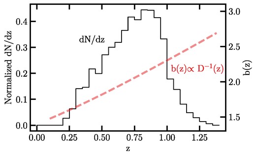
The redshift distribution (solid line and vertical scale on the left) and bias evolution (dashed line and vertical scale on the right) of the DESI LRG targets. The redshift distribution is determined from DESI spectroscopy (DESI Collaboration 2024). The redshift evolution of the linear bias is supported by halo occupation distribution (HOD) fits to the angular clustering of the DESI LRG targets (Zhou et al. 2021), where D(z) represents the growth factor.
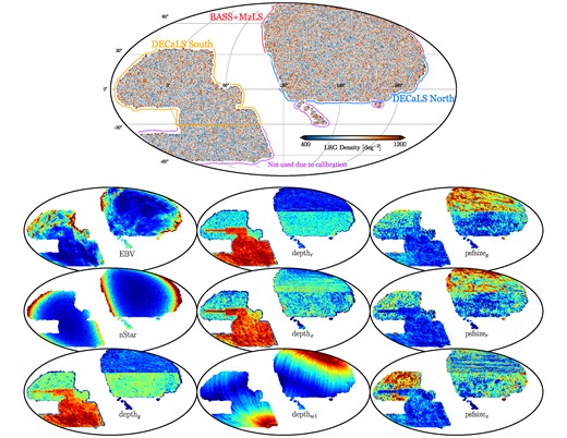
Top: the DESI LRG target density map before correcting for imaging systematic effects in Mollweide projection. The disconnected islands from the North footprint and parts of the South footprint with declination below −30 are removed from the sample for the analysis due to potential calibration issues (see the text). Bottom: Mollweide projections of the imaging systematic maps (survey depth, astronomical seeing/psfsize, Galactic extinction, and local stellar density) in celestial coordinates. Not shown here are two external maps for the neutral hydrogen column density and photometric calibration, which are only employed for the robustness tests.
2.1 DESI imaging LRGs
Our sample of LRGs is drawn from the DESI Legacy Imaging Surveys Data Release 9 (DR9; Dey et al. 2019) using the colour–magnitude selection criteria designed for the DESI 1 per cent survey (DESI Collaboration 2024), described as the Survey Validation 3 (SV3) selection in more detail in Zhou et al. (2023a). The colour–magnitude selection cuts are defined in the g, r, z bands in the optical and W1 band in the infrared, as summarized in Table 1. The selection cuts vary for each imaging survey, but they are designed to achieve a nearly consistent density of approximately 800 galaxies per deg2 across a total area of roughly |$14\, 000$| deg2. Table 2 summarizes the mean galaxy density and area for each region. This is accomplished despite variations in survey efficiency and photometric calibration between DECaLS and BASS + MzLS. The implementation of these selection cuts in the DESI data processing pipeline is explained in Myers et al. (2023). The redshift distribution of our galaxy sample are inferred respectively from DESI spectroscopy during the SV phase (DESI Collaboration 2024), and is shown via the solid curve in Fig. 1. Zhou et al. (2021) analysed the DESI LRG targets and found that the redshift evolution of the linear bias for these targets is consistent with a constant clustering amplitude and varies via 1/D(z), where D(z) is the growth factor (as illustrated by the dashed red line in Fig. 1).
Colour–magnitude selection criteria for the DESI LRG targets (Zhou et al. 2023a). Magnitudes are corrected for Galactic extinction. The z-band fibre magnitude, zfibre, corresponds to the expected flux within a DESI fibre.
| Footprint | Criterion | Description |
|---|---|---|
| zfibre < 21.7 | Faint limit | |
| DECaLS | z − W1 > 0.8 × (r − z) − 0.6 | Stellar rejection |
| [(g − r > 1.3) AND ((g − r) > −1.55*(r − W1) + 3.13)] OR (r − W1 > 1.8) | Remove low-z galaxies | |
| [(r − W1 > (W1 − 17.26)*1.8) AND (r − W1 > W1 − 16.36)] OR (r − W1 > 3.29) | Luminosity cut | |
| zfibre < 21.71 | Faint limit | |
| BASS + MzLS | z − W1 > 0.8 × (r − z) − 0.6 | Stellar rejection |
| [(g − r > 1.34) AND ((g − r) > −1.55*(r − W1) + 3.23)] OR (r − W1 > 1.8) | Remove low-z galaxies | |
| [(r − W1 > (W1 − 17.24)*1.83) AND (r − W1 > W1 − 16.33)] OR (r − W1 > 3.39) | Luminosity cut |
Statistics for DESI imaging data. Median depths are for galaxy/point sources detected at 5σ. Median psfsize values are computed with a depth-weighted average at each location on the sky.
| BASS + MzLS | DECaLS North | DECaLS South | |
|---|---|---|---|
| Mean galaxy density (deg−2) | 804 | 808 | 796 |
| Area (deg2) | 4525 | 5257 | 5188 |
| Median extinction (mag) | 0.02 | 0.03 | 0.05 |
| Median stellar density (deg−2) | 667 | 629 | 629 |
| Median g galaxy depth (mag) | 24.0 | 24.4 | 24.5 |
| Median r galaxy depth (mag) | 23.4 | 23.8 | 23.9 |
| Median z galaxy depth (mag) | 23.0 | 22.9 | 23.1 |
| Median W1 psf depth (mag) | 21.6 | 21.4 | 21.4 |
| Median g psfsize (arcsec) | 1.9 | 1.5 | 1.5 |
| Median r psfsize (arcsec) | 1.7 | 1.4 | 1.3 |
| Median z psfsize (arcsec) | 1.2 | 1.3 | 1.3 |
The LRG sample is masked rigorously for foreground bright stars, bright galaxies, and clusters of galaxies1 to further reduce stellar contamination (Zhou et al. 2023a). Then, the sample is binned into healpix (Gorski et al. 2005) pixels at |${\small NSIDE}=256$|, corresponding to pixels of about 0.25° on a side, to construct the 2D density map (as shown in the top panel of Fig. 2). The LRG density is corrected for the pixel incompleteness and lost areas using a catalogue of random points, hereafter referred to as randoms, uniformly scattered over the footprint with the same cuts and masks applied. Moreover, the density of galaxies is matched to the randoms separately for each of the three data sections (BASS + MzLS, DECaLS North/South) so the mean density differences are mitigated (see Table 2). The DESI LRG targets are selected brighter than the imaging survey depth limits, for example, g = 24.4, r = 23.8, and z = 22.9 for the median 5σ detection in AB mag in the DECaLS North region (Table 2); and thus the LRG density map does not exhibit severe spurious fluctuations.
2.1.1 Imaging systematic maps
The effects of observational systematics in the DESI targets have been studied in great detail (see e.g. Kitanidis et al. 2020; Zhou et al. 2021; Chaussidon et al. 2022). Zhou et al. (2023a) have previously identified nine astrophysical properties as potential sources of imaging systematic errors in the DESI LRG targets. These imaging properties are mapped into healpix of nside=256. As illustrated by the 3 × 3 grid in the bottom panel of Fig. 2, the maps include local stellar density constructed from point-like sources with a G-band magnitude in the range 12 ≤ G < 17 from the Gaia DR2 (see Gaia Collaboration 2018; Myers et al. 2023); Galactic extinction E(B−V) from Schlegel, Finkbeiner & Davis (1998); survey depth (galaxy depth in g, r, and z and PSF depth in W1) and astronomical seeing (i.e. point spread function, or psfsize) in g, r, and z. The depth maps have been corrected for extinction using the coefficients adapted from Schlafly & Finkbeiner (2011). Table 2 summarizes the median values for the imaging properties in each region. In addition to these nine maps, we consider two external maps for the neutral hydrogen column density (H i) from HI4PI Collaboration (2016) and photometric calibration in the z band (CALIBZ) from DESI Collaboration (2024) to further test the robustness of our analysis against unknown systematics.
The fluctuations in each imaging map are unique and tend to be correlated with the LRG density map. For instance, large-scale LRG density fluctuations could be caused by stellar density, extinction, or survey depth; while small-scale fluctuations could be caused by psfsize variations. Some regions of the DR9 footprint are removed from our analysis to avoid potential photometric calibration issues. These regions are either disconnected from the main footprint (e.g. the islands in the NGC with Dec. <−10) or calibrated using different catalogues of standard stars (e.g. Dec. <−30 in the SGC). The potential impact of not imposing these declination cuts on the LRG sample and our fNL constraints is explored in Section 4.
We employ the Pearson correlation coefficient to characterize the correlation between the galaxy density and imaging properties, which for two random variables x and y is given by,
where |$\bar{x}$| and |$\bar{y}$| represent the mean estimates of the random variables. Fig. 3 shows the Pearson correlation coefficient between the DESI LRG target density map and the imaging systematics maps for the three imaging regions (DECaLS North, DECaLS South, and BASS + MzLS) in the top panel. The horizontal curves represent the |$95{{\ \rm per\ cent}}$| confidence regions for no correlation and are constructed by cross-correlating 100 synthetic lognormal density fields, generated with fNL = 0, and the imaging systematic maps. Consistent among the different regions, there are statistically significant correlations between the LRG density and depth, extinction, and stellar density. There are less significant correlations between the LRG density and the W1-band depth and psfsize. The signs of the correlations imply that there are more targets where extinction is high, and less targets where depth is high. Another interpretation might be that more contaminants are targeted where depth is shallow. Fig. 3 (bottom panel) shows the correlation matrix among the imaging systematic maps for the entire DESI footprint. Significant inner correlations exist among the imaging systematic maps themselves, especially between local stellar density and Galactic extinction; also, the r- and g-band survey properties are more correlated with each other than with the z-band counterpart. Additionally, we compute the Spearman correlation coefficients between the LRG density and imaging systematic maps to assess whether or not the correlations are impacted by outliers in the imaging data, but find no substantial differences from Pearson.
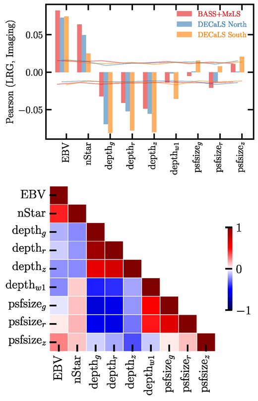
Top: the Pearson correlation coefficient between the DESI LRG target density and imaging properties in BASS + MzLS, DECaLS North, and DECaLS South. Solid horizontal curves represent the |$95{{\ \rm per\ cent}}$| confidence intervals estimated from simulations of lognormal density fields with fNL = 0. Bottom: the Pearson correlation matrix of imaging properties for the DESI footprint.
2.1.2 Treatment of imaging systematics
There are several approaches for handling imaging systematic errors, broadly classified into data-driven and simulation-based modelling approaches (see e.g. Ross et al. 2011, 2012, 2017; Ho et al. 2012; Suchyta et al. 2016; Delubac et al. 2016; Prakash et al. 2016; Raichoor et al. 2017; Laurent et al. 2017; Elvin-Poole et al. 2018; Bautista et al. 2018; Rezaie et al. 2020, 2021; Kong et al. 2020; Everett et al. 2022; Chaussidon et al. 2022; Eggert & Leistedt 2023). The general idea behind these approaches is to use the available data or simulations to learn or forward model the relationship between the observed target density and the imaging systematic maps, and to use this relationship, which is often described by a set of imaging weights, to mitigate spurious fluctuations in the observed target density. Another techniques for reducing the effect of imaging systematics rely on cross-correlating different tracers of dark matter to ameliorate excess clustering signals, as each tracer might respond differently to a source of systematic error (see e.g. Giannantonio et al. 2014). These methods have their limitations and strengths (see e.g. Weaverdyck & Huterer 2021, for a review). In this paper, data-driven approaches, including linear multivariate regression and artificial neural networks, are applied to the data to correct for imaging systematic effects.
2.1.2.1 Linear multivariate model
The linear multivariate model only uses the imaging systematic maps up to the linear power to predict the number counts of the DESI LRG targets in pixel i,
where a0 is a global offset, and a · xi represents the inner product between the parameters, a, and the values for imaging systematics in pixel i, xi. The Softplus functional form for Ni is adapted to force the predicted galaxy counts to be positive (Dugas et al. 2001). Then, Markov Chain Monte Carlo (MCMC) search is performed using the emcee package (Foreman-Mackey et al. 2013) to explore the parameter space by minimizing the negative Poisson log-likelihood between the actual and predicted number counts of galaxies.
Spatial coordinates are not included in xi to help avoid overcorrection. As a result, the predicted number counts solely reflect the spurious density fluctuations that arise from varying imaging conditions. The number of pixels is substantially larger than the number of parameters for the linear model, and thus no training-validation-testing split is applied to the data for training the linear model. This aligns with the methodology used for training linear models in previous analyses (see e.g. Zhou et al. 2023a). The predicted galaxy counts are evaluated for each region using the marginalized mean estimates of the parameters, combined with those from other regions to cover the DESI footprint. The linear-based imaging weights are then defined as the inverse of the predicted target density, normalized to a median of unity.
2.1.2.2 Neural network model
Our neural network-based mitigation approach uses the implementation of fully connected feedforward neural networks from Rezaie et al. (2021). With the neural network approach, a · xi in equation (3) is replaced with NN(xi|a), where NN represents the fully connected neural network and a denotes its parameters. The implementation, training, validation, and application of neural networks on galaxy survey data are presented in Rezaie et al. (2021). We briefly summarize the methodology here.
A fully connected feedforward neural network (also called a multilayer perceptron) is a type of artificial neural network where the neurons are arranged in layers, and each neuron in one layer is connected to every neuron in the next layer. The imaging systematic information flows only in one direction, from input to output. Each neuron applies a non-linear activation function (i.e. transformation) to the weighted sum of its inputs, which are the outputs of the neurons in the previous layer. The output of the last layer is the model prediction for the number counts of galaxies. Our architecture consists of three hidden layers with 20 rectifier activation functions on each layer, and a single neuron in the output layer. The rectifier is defined as max(0, x) to introduce non-linearities in the neural network (Nair & Hinton 2010). This simple form of non-linearity is very effective in enabling deep neural networks to learn more complex, non-linear relationships between the input imaging maps and output galaxy counts.
Compared with linear regression, neural networks potentially are more prone to overfitting, that is, excellent performance on training data and poor performance on validation (or test) data. Therefore, our analysis uses a training-validation-testing split to avoid overfitting and ensure that the neural network is well optimized. Specifically, |$60{{\ \rm per\ cent}}$| of the LRG data is used for training, |$20{{\ \rm per\ cent}}$| is used for validation, and |$20{{\ \rm per\ cent}}$| is used for testing. The split is performed randomly aside from the locations of the pixels. We also test a geometrical split in which neighbouring pixels belong to the same set of training, testing, or validation, but no significant performance difference is observed.
The neural networks are trained for up to 70 training epochs with the gradient descent adam optimizer (Loshchilov & Hutter 2017), which iteratively updates the neural network parameters following the gradient of the negative Poisson log-likelihood. The step size of the parameter updates is controlled via the learning rate hyperparameter, which is initialized with a grid search and is designed to dynamically vary between two boundary values of 0.001 and 0.1 to avoid local minima (see again, Loshchilov & Hutter 2016). At each training epoch, the neural network model is applied to the validation set, and ultimately the model with the best performance on validation is identified and applied to the test set. The neural network models are tested on the entirety of the LRG sample with the technique of permuting the choice of the training, validation, or testing sets (Arlot & Celisse 2010). With the cross-validation technique, the model predictions from the different test sets are aggregated together to form the predicted target density map into the DESI footprint. To reduce the error in the predicted number counts, we train an ensemble of 20 neural network models and average over the predictions. The imaging weights are then defined as the inverse of the predicted target density, normalized to a median of unity.
2.2 Synthetic lognormal density fields
Density fluctuations of galaxies on large scales can be approximated with lognormal distributions (Coles & Jones 1991; Clerkin et al. 2017). Unlike N-body simulations, simulating lognormal density fields is not computationally intensive, and allows quick and robust validation of data analysis pipelines. Lognormal simulations are therefore considered efficient for our study since the signature of local PNG appears on large- and small-scale clustering is not used in our analysis. The package flask (Full-sky Lognormal Astro-fields Simulation Kit; Xavier, Abdalla & Joachimi 2016) is employed to generate ensembles of synthetic lognormal density maps that mimic the bias, redshift, and angular distributions of the DESI LRG targets, as illustrated in Figs 1 and 2. Two universes with fNL = 0 and 76.9 are considered. A set of 1000 realizations is produced for every fNL. The mocks are designed to match the clustering signal of the DESI LRG targets on scales insensitive to fNL. The analysis adapts the fiducial Baryon Oscillation Spectroscopic Survey cosmology (BOSS Collaboration 2017) which assumes a flat lambda-cold dark matter universe, including one massive neutrino with mν = 0.06 eV, Hubble constant h = 0.68, matter density ΩM = 0.31, baryon density Ωb = 0.05, and spectral index ns = 0.967. The amplitude of the matter density fluctuations on a scale of 8 h−1Mpc is set as σ8 = 0.8225. The same fiducial cosmology is used throughout this paper unless specified otherwise. Our robustness tests show that the none of the cosmological parameters can produce an fNL-like signatures, and therefore, our analysis is not sensitive to the choice of fiducial cosmology.
2.2.1 Contaminated mocks
We employ the linear multivariate model (equation 3) to introduce synthetic spurious fluctuations in the lognormal density fields, and validate our imaging systematic mitigation methods. The motivation for choosing a linear contamination model is to assess how much of the clustering signal can be removed by applying more flexible models, based on neural networks, for correcting less severe imaging systematic effects. The imaging systematic maps considered for the contamination model are extinction, depth in z, and psfsize in r. As shown in the Pearson correlation (Fig. 3) and will be discussed later in Section 3.4, the DESI LRG targets correlate strongly with these three maps. We fit for the parameters of the linear models with the MCMC process, executed separately on each imaging survey (BASS + MzLS, DECaLS North, and DECaLS South). Then, the imaging selection function for contaminating each simulation is uniquely determined by randomly drawing from the parameter space probed by MCMC, and then the results from each imaging survey are combined to form the DESI footprint. The clean density is then multiplied by the contamination model to induce systematics. The same contamination model is used for both the fNL = 0 and 76.9 simulations.
Similar to the imaging systematic treatment analysis for the DESI LRG targets, the neural network methods with various combinations of the imaging systematic maps are applied to each simulation, with and without PNG, and with and without systematics, to derive the imaging weights. Section 3 presents how the simulation results are incorporated to calibrate fNL biases due to overcorrection. We briefly summarize two statistical tests based on the mean galaxy density contrast and the cross power spectrum between the galaxy density and the imaging systematic maps to assess the quality of the data and the significance of the remaining systematic effects (see also Rezaie et al. 2021). We calculate these statistics and compare the values to those measured from the clean mocks before looking at the auto power spectrum of the DESI LRG targets.
3 ANALYSIS TECHNIQUES
We address imaging systematics in DESI data by performing a separate treatment for each imaging region (e.g. DECaLS North) within the DESI footprint to reduce the impact of systematic effects specific to that region. Once the imaging systematic weights are obtained for each imaging region separately, we combine the data from all regions to compute the power spectrum for the entire DESI footprint to increase the overall statistical power and enable more robust measurements of fNL. We then conduct robustness tests on the combined data to assess the significance of any remaining systematic effects.
3.1 Power spectrum estimator
We first construct the density contrast field from the LRG density, ρ,
where the mean galaxy density |$\overline{\rho }$| is estimated from the entire LRG sample. As a robustness test, we also analyse the power spectrum from each imaging region individually, in which |$\overline{\rho }$| is calculated separately for each region. Then, we use the pseudo-angular power spectrum estimator (Hivon et al. 2002),
where the coefficients aℓm are obtained by decomposing δg into spherical harmonics, Yℓm,
where W represents the survey window that is described by the number of randoms normalized to the expected value.
We use the implementation of anafast from the healpix package (Gorski et al. 2005) to do fast harmonic transforms (equation 6) and estimate the pseudo-angular power spectrum of the LRG targets and the cross-power spectrum between the LRG targets and the imaging systematic maps.
3.2 Modelling
The estimator in equation (5) yields a biased power spectrum when the survey sky coverage is incomplete. Specifically, the survey mask causes correlations between different harmonic modes (Beutler et al. 2014; Wilson et al. 2017), and the measured clustering power is smoothed on scales near the survey size. An additional potential cause of systematic error arises from the fact that the mean galaxy density used to construct the density contrast field (equation 4) is estimated from the available data, rather than being known a priori. This introduces what is known as an integral constraint effect, which can cause the power spectrum on modes near the size of the survey to be artificially suppressed, effectively pushing it towards zero (Peacock & Nicholson 1991; De Mattia & Ruhlmann-Kleider 2019). Since fNL is highly sensitive to the clustering power on these scales, it is crucial to account for these systematic effects in the model galaxy power spectrum to obtain unbiased fNL constraints (see also Riquelme et al. 2023), which we describe below.
The other theoretical systematic issues are however subdominant in the angular power spectrum. For instance, relativistic effects generate PNG-like scale-dependent signatures on large scales, which interfere with measuring fNL with the scale-dependent bias effect using higher order multipoles of the 3D power spectrum (Wang, Beutler & Bacon 2020). Similarly, matter density fluctuations with wavelengths larger than survey size, known as supersample modes, modulate the galaxy 3D power spectrum (Castorina & Moradinezhad Dizgah 2020). In a similar way, the peculiar motion of the observer can mimic a PNG-like scale-dependent signature through aberration, magnification and the Kaiser–Rocket effect, that is, a systematic dipolar apparent blueshifting in the direction of the observer’s peculiar motion (Bahr-Kalus et al. 2021).
3.2.1 Angular power spectrum
The relationship between the linear matter power spectrum P(k) and the projected angular power spectrum of galaxies is expressed by the following equation:
where Nshot is a scale-independent shot noise term. The projection kernel |$\Delta _{\ell }(k) = \Delta ^{\rm g}_{\ell }(k) + \Delta ^{\rm RSD}_{\ell }(k) + \Delta ^{\mu }_{\ell }(k)$| includes redshift space distortions and magnification bias, and determines the contribution of each wavenumber k to the galaxy power spectrum on mode ℓ. For more details on this estimator, refer to Padmanabhan et al. (2007). The non-linearities in the matter power spectrum are negligible for the scales of interest (see e.g. Ho et al. 2015). For ℓ = 40, Δℓ(k) peaks at k ∼ 0.02 h Mpc−1, which is above the non-linear regime. The FFTLog algorithm and its extension2 as implemented in Fang et al. (2020) are employed to calculate the integrals for the projection kernel Δℓ(k), which includes the lth-order spherical Bessel functions, jℓ(kr), and its second derivatives,
where b is the linear bias (dashed curve in Fig. 1), D represents the linear growth factor normalized as D(z = 0) = 1, f(r) is the growth rate, and dN/dr is the redshift distribution of galaxies normalized to unity and described in terms of comoving distance3 (solid curve in Fig. 1). The magnification bias window function Wμ(z) is
where Ωm is the matter density, H0 is the Hubble constant,4c is the speed of light, and s represents the slope of the number count function, a metric quantifying the response of the number density of galaxies to achromatic changes in brightness (Loverde, Hui & Gaztañaga 2008). The estimation of s involves shifting all magnitudes by an infinitesimal amount and re-running the colour–magnitude selection. Zhou et al. (2023b) developed a strategy to estimate s for a fibre flux-selected sample like the DESI LRG targets, for which the impact of magnification on fibre flux depends on the shape parameters for each morphology type. Following the same strategy, the parameter s is re-calculated for our selection of the DESI LRGs (DESI SV3):5s = 0.951 ± 0.011 for BASS + MzLS, s = 0.943 ± 0.007 for DECaLS North + DECaLS South, and s = 0.945 ± 0.006 for DESI. For consistency, we fix s to the above central values in our analysis.
The PNG-induced scale-dependent shift is given by (Slosar et al. 2008)
where T(k) is the transfer function, and g(∞)/g(0) ∼ 1.3 with g(z) ≡ (1 + z)D(z) is the growth suppression due to non-zero Λ because of our normalization of D (see e.g. Reid et al. 2010; Mueller, Percival & Ruggeri 2019). We assume the universality relation which directly relates bϕ to b via bϕ = 2δc(b − p) with δc = 1.686 representing the critical density for spherical collapse (Fillmore & Goldreich 1984). We fix p = 1 in our analysis and marginalize over b (see also Slosar et al. 2008; Reid et al. 2010; Ross et al. 2013).
3.2.2 Survey geometry and integral constraint
We employ a technique similar to the one proposed by Chon et al. (2004) to account for the impact of the survey geometry on the theoretical power spectrum. The ensemble average for the partial sky power spectrum is related to that of the full sky power spectrum via a mode–mode coupling matrix, |${\rm M}_{\ell \ell ^{\prime }}$|,
We convert this convolution in the spherical harmonic space into a multiplication in the correlation function space. Specifically, we first transform the theory power spectrum (equation 7) to the correlation function, |$\hat{\omega }^{\rm model}$|. Then, we estimate the survey mask correlation function, |$\hat{\omega }^{\rm window}$|, and obtain the pseudo-power spectrum,
Fig. 4 illustrates the survey mask correlation function |${\hat{\omega }}^{\rm window}$| for various masks representing the DESI footprint and its imaging subregions. Appendix A2 shows the validation of our method by comparing it to an alternative approach that computes the mode–mode coupling matrix |${\rm M}_{\ell \ell ^{\prime }}$| and performs the convolution (equation 13) directly in ℓ-space. We notice as the fNL deviates from zero, our approach introduces a noisy feature in the model, qualitatively in an unbiased manner (ΔfNL < 1.1). Fig. B2 indeed demonstrates that our approach can recover the truth fNL in spite of the noisy feature.
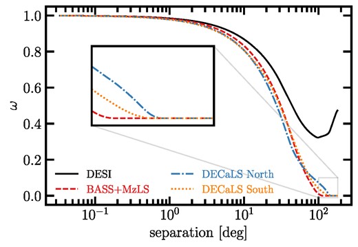
The survey mask correlation functions across the imaging regions forming the DESI footprint, plotted against angular separation. The inset focuses on correlations within the angular range of 100°–180°.
The integral constraint is anothe error on the mean and one realization, respectively. No imaging systematic cleaning is applied to these mocks.r systematic effect which is induced since the mean galaxy density is estimated from the observed galaxy density, and therefore is biased by the limited sky coverage (Peacock & Nicholson 1991). To account for the integral constraint, the survey mask power spectrum is used to introduce a scale-dependent correction factor that needs to be subtracted from the power spectrum as,
where |$\tilde{C}^{\rm window}$| is the survey mask power spectrum, that is, the spherical harmonic transform of |$\hat{\omega }^{\rm window}$|.
The lognormal simulations are used to validate the survey window and integral constraint correction. Fig. 5 shows the mean power spectrum of the fNL = 0 simulations (dashed) and the best-fitting theory prediction before and after accounting for the survey mask and integral constraint. The simulations are neither contaminated nor mitigated. The light and dark shades represent the 68 per cent estimated error on the mean and one single realization, respectively. The DESI mask, which covers around |$40{{\ \rm per\ cent}}$| of the sky, is applied to the simulations. We find that the survey window effect modulates the clustering power on ℓ < 200 and the integral constraint alters the clustering power on ℓ < 6.
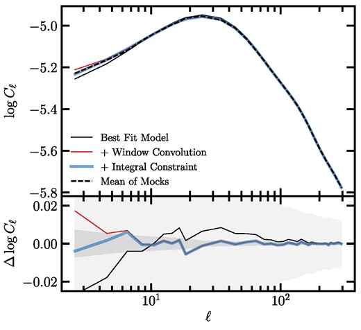
The mean power spectrum from the fNL = 0 mocks (no contamination) and best-fitting theoretical prediction after accounting for the survey geometry and integral constraint effects. Bottom panel shows the residual power spectrum relative to the mean power spectrum. The dark and light shades represent the 68 per cent error on the mean and one realization, respectively. No imaging systematic cleaning is applied to these mocks.
3.3 Parameter estimation
Our parameter inference uses standard MCMC sampling. A constant clustering amplitude is assumed to determine the redshift evolution of the linear bias of the DESI LRG targets, b(z) = b/D(z), which is supported by the HOD fits to the angular power spectrum (Zhou et al. 2021). In MCMC, we allow fNL, Nshot, and b to vary, while all other cosmological parameters are fixed at the fiducial values (see Section 2.2). The galaxy power spectrum is divided into a discrete set of bandpower bins with Δℓ = 2 between ℓ = 2 and 20 and Δℓ = 10 from ℓ = 20 to 300. Each clustering mode is weighted by 2ℓ + 1 when averaging over the modes in each bin.
The expected large-scale power is highly sensitive to the value of fNL such that the the amplitude of the covariance for Cℓ is influenced by the true value of fNL, see also Ross et al. (2013) for a discussion. As illustrated in the top row of Fig. 6, we find that the distribution of the power spectrum at the lowest bin, 2 ≤ ℓ < 4, is highly asymmetric and its standard deviation varies significantly from the simulations with fNL = 0 to 76.9. We can make the covariance matrix less sensitive to fNL by taking the log transformation of the power spectrum, log Cℓ. As shown in the bottom panels in Fig. 6, the log transformation reduces the asymmetry and the difference in the standard deviations between the fNL = 0 and 76.9 simulations. Therefore, we minimize the negative log likelihood defined as,
where Θ represents a container for the parameters fNL, b, and Nshot; |$\tilde{C}(\Theta)$| is the (binned) expected pseudo-power spectrum; |$\tilde{C}$| is the (binned) measured pseudo-power spectrum; and |$\mathbb {C}$| is the covariance on |$\log \tilde{C}$| constructed from the fNL = 0 lognormal simulations. Lognormal simulations have been commonly used and validated to estimate the covariance matrices for galaxy density fields, and non-linear effects are subdominant on the scales of interest to fNL (see e.g. Clerkin et al. 2017; Friedrich et al. 2021). We also test for the robustness of our results against an alternative covariance constructed from the fNL = 76.9 mocks. Flat priors are implemented for all parameters: fNL ∈ [ − 1000, 1000], Nshot ∈ [ − 0.001, 0.001], and b ∈ [0, 5].
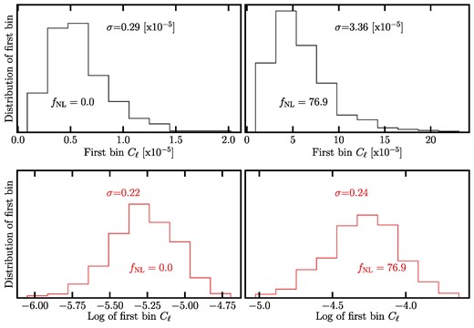
The distribution of the first bin power spectra and its log transformation from the simulations with fNL = 0 (left) and 76.9 (right). The log transformation largely removes the asymmetry in the distributions.
3.4 Characterization of remaining systematics
One potential problem that can arise in the data-driven mitigation approach is overcorrection, which occurs when the corrections applied to the data remove the clustering signal and induce additional biases in the inferred parameter of interest. The neural network approach is more prone to this issue compared to the linear approach due to its increased degrees of freedom. As illustrated in the bottom panel of Fig. 3, the significant correlations among the imaging systematic maps may pose additional challenges for modelling the spurious fluctuations in the galaxy density field. Specifically, using highly correlated imaging systematic maps increases the statistical noise in the imaging weights, which elevates the potential for over subtracting the clustering power. These overcorrection effects are estimated to have a negligible impact on baryon acoustic oscillations (Merz et al. 2021); however, they can significantly modulate the galaxy power spectrum on large scales, and thus lead to biased fNL constraints (Rezaie et al. 2021; Mueller et al. 2022). Although not explored thoroughly, the overcorrection issues could limit the detectability of primordial features in the galaxy power spectrum and that of parity violations in higher order clustering statistics (Beutler et al. 2019; Cahn, Slepian & Hou 2021; Philcox 2022). Therefore, it is crucial to develop, implement, and apply techniques to minimize and control overcorrection in the hope of ensuring that the constraints are as accurate and reliable as possible; one such approach is to reduce the dimensionality of the problem. Our goal is to reduce the correlations between the DESI LRG target density and the imaging systematic maps while controlling the overcorrection effect. In this section, we describe how we approach this objective, by employing a series of simulations along with the residual systematics that we construct based on the cross power spectrum between the LRG density and imaging maps, and the mean LRG density as a function of imaging. We test different sets of the imaging systematic maps to identify the optimal set of the feature maps:
Two maps: extinction, depth in z.
Three maps: extinction, depth in z, psfsize in r.
Four maps: extinction, depth in z, psfsize in r, stellar density.
Eight maps: extinction, depth in grzW1, psfsize in grz.
Nine maps: extinction, depth in grzW1, psfsize in grz, stellar density.
Eleven maps: same as Nine maps but with two additional maps; extinction, depth in grzW1, psfsize in grz, stellar density, neutral hydrogen density, and photometric calibration in z.
It is imperative to note that these sets are selected prior to examining the auto power spectrum of the LRG sample and unblinding the fNL constraints, and that the auto power spectrum and fNL measurements are unblinded only after our mitigation methods passed our rigorous tests for residual systematics. As detailed in Section 3.4, we discover that these tests tend to depend on the fNL value which is used in the mocks for the covariance matrix estimation.
3.4.1 Normalized cross power spectrum
We characterize the cross-correlations between the galaxy density and imaging systematic maps by
where |$\tilde{C}_{x_{i}, \ell }$| represents the the square of the cross power spectrum between the galaxy density and ith imaging map, xi, divided by the auto power spectrum of xi:
With this normalization, |$\tilde{C}_{x_{i}, \ell }$| estimates the contribution of systematics at every multipole up to the linear order to the galaxy power spectrum. Then, the χ2 value for the cross power spectra is calculated via,
where the covariance matrix |$\mathbb {C}_{X} = \lt \tilde{C}_{X, \ell } \tilde{C}_{X, \ell ^{\prime }} \gt $| is constructed from the lognormal mocks. We consider both sets with fNL = 0 and 76.9, and for each mitigated case, the covariance is from the mocks that have received the same treatment. These χ2 values are measured for every clean mock realization with the leave-one-out technique and compared to the values observed in the DESI LRG targets with various imaging systematic corrections. Specifically, we use 999 realizations to estimate a covariance matrix and then apply the covariance matrix from the 999 realizations to measure the χ2 for the one remaining realization. This process is repeated for all 1000 realizations to construct a histogram for χ2. We only include the bandpower bins from ℓ = 2 to 20 with Δℓ = 2, which results in a total of 81 bins, and test for the robustness with higher ℓ modes in A1.
Fig. 7 shows |$\tilde{C}_{X,\ell }$| from the DESI LRG targets before and after applying various corrections for imaging systematics. The dark and light shades show the 97.5th percentile from the fNL = 0 and 76.9 mocks, respectively, that have had no mitigation applied to them. Without imaging weights (No Weight), the DESI LRG targets have the highest cross-correlations against extinction, stellar density, and depth in z. There are less significant correlations against depth in the g and r bands, and psfsize in the z band, which could be driven because of the inner correlations between the imaging systematic maps. First, we consider cleaning the DESI LRG targets with the linear model using two maps (extinction and depth in z) as identified from the Pearson correlation. Linear two maps is the least aggressive treatment method in terms of both the model flexibility and the number of input maps. With linear two maps, most of the cross-correlation signals are reduced below statistical uncertainties, especially against extinction, stellar density, and depth. However, the cross-correlations against psfsize in the r and z bands increase slightly on 6 < ℓ < 20 and 6 < ℓ < 14, respectively. This might be indicative of residual trends against psfsize.
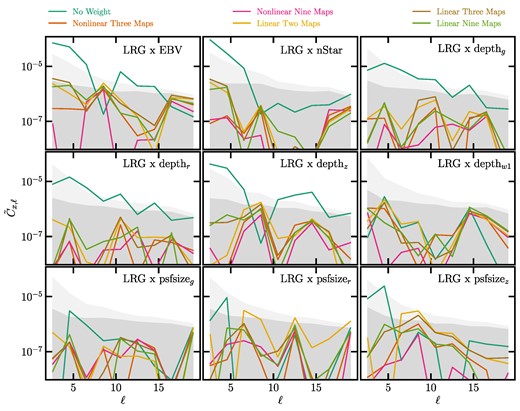
The square of the cross power spectra between the DESI LRG targets and imaging systematic maps normalized by the auto power spectrum of the imaging systematic maps; see equation (18). The systematic maps considered are Galactic extinction (EBV), stellar density (nStar), depth in grzw1 (depthgrzw1), and seeing in grz (psfsizegrz). The dark green curves display the cross spectra before imaging systematic correction (No Weight). The yellow, brown, and light green curves represent the results after applying the imaging weights from the linear models trained with two maps, three maps, and nine maps. The orange and purple curves display the results after applying the imaging weights from the non-linear models trained with three maps and nine maps. The dark and light shades represent the 97.5 percentile from cross-correlating the imaging systematic maps and the fNL = 0 and 76.9 lognormal density fields, respectively, without mitigation.
The linear three maps approach alleviates the cross-correlation against psfsize in r, and it yields similar results to those obtained from linear nine maps, which indicates most of the contaminations can be attributed to these three maps. Therefore, we identify extinction, depth in z, and psfsize in r (three maps) as the primary sources of systematic effects in the DESI LRG targets. Then, we adapt neural network three maps to model non-linear systematic effects. Compared with the linear three maps method, we find that non-linear three maps can reduce the cross-correlations against both the r- and z-band psfsize maps, which shows the benefit of using a non-linear approach. To further examine the robustness of our cleaning methods, we also show the cross-correlations after cleaning the DESI LRG targets using nine imaging property maps (non-linear nine maps). We do not find any significant residuals against the two extra maps for the neutral hydrogen density and photometric calibration in thez band.
3.4.2 Mean galaxy density contrast
We calculate the histogram of the mean galaxy density contrast relative to the jth imaging property, xj:
where |$\overline{\rho }$| is the global mean galaxy density, Wi is the survey window in pixel i, and the summations over i are evaluated from the pixels in every bin of xj. We compute the histograms against all nine imaging properties (see Fig. 2). We use a set of eight equal width bins for every imaging map, which results in a total of 72 bins. Then, we construct the total mean density contract as,
and the total residual error as,
where the covariance matrix |$\mathbb {C}_{\delta } = \lt \delta _{X} \delta _{X}\gt $| is constructed from the lognormal mocks, in a consistent manner similar to the normalized cross power spectrum. Fig. 8 shows the mean density contrast against the imaging properties for the DESI LRG targets. The dark and light shades represent the 1σ level fluctuations observed in 1000 lognormal density fields respectively with fNL = 0 and 76.9 before mitigation. The DESI LRG targets before treatment (No Weight) exhibits a strong trend around |$10{{\ \rm per\ cent}}$| against the z-band depth which is consistent with the cross power spectrum. Additionally, there are significant spurious trends against extinction and stellar density at about |$5\,\mathrm{ per\,cent}-6{{\ \rm per\ cent}}$|. The linear approach is able to mitigate most of the systematic fluctuations with only extinction and depth in the z band as input; however, a new trend appears against the r-band psfsize map with the linear two maps approach, which is indicative of the psfsize-related systematics in the DESI LRG targets. This finding is in agreement with that from the cross power spectrum test. With linear three maps, we still observe around |$2{{\ \rm per\ cent}}$| residual spurious fluctuations in the low end of depth in z and around |$1{{\ \rm per\ cent}}$| in the high end of psfsize in z, which implies the presence of non-linear systematic effects. We find that the imaging weights from the non-linear model trained with the three identified maps (or four maps including the stellar density) are capable of reducing the fluctuations below |$2{{\ \rm per\ cent}}$|. Even with the non-linear three maps, we have about |$1{{\ \rm per\ cent}}$| remaining systematic fluctuations against the z-band psfsize. The spurious trends are diminished especially when we adapt non-linear nine maps, especially against the low end of depth in g and r and against the high end of psfsize in z.
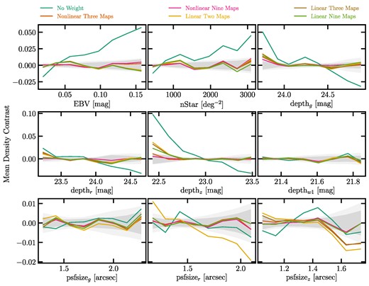
The mean density contrast of the DESI LRG targets as a function of the imaging systematic maps: Galactic extinction (EBV), stellar density (nStar), depth in grzw1 (depthgrzw1), and seeing in grz (psfsizegrz). The black curves display the results before imaging systematic correction. The red, blue and orange curves represent the relationships after applying the imaging weights from the linear models trained with two maps, three maps, and eight maps, respectively. The green and pink curves display the results after applying the imaging weights from the non-linear models trained with three maps and four maps. The dark and light shades represent the |$68{{\ \rm per\ cent}}$| dispersion of 1000 lognormal mocks with fNL = 0 and 76.9, respectively.
3.4.3 Residual error χ2
We use the χ2 statistics to quantitatively assess how significant these mean density and cross power spectrum fluctuations are in comparison to the clean mocks. Fig. 9 presents χ2 histograms for the mean density contrast (left) and the normalized cross spectrum (right) statistics obtained from the lognormal mocks with different fNL values before and after applying mitigation methods. The mocks with fNL = 0 are shown with the solid curves while the other set with fNL = 76.9 are represented with the dashed curves. The use of the self-consistent covariance matrix (with respect to fNL or mitigation method) results in similar distributions, and therefore the mock histograms are employed as reference to evaluate the significance of residual systematics in the DESI LRG targets. We continue to use the self-consistent covariance, but consider both the fNL = 0 and 76.9 covariance. The DESI LRG target χ2 values are compared via the vertical lines and summarized in Table 3. The solid and dashed vertical lines represent the values computed using the covariances based on the fNL = 0 and 76.9 mocks, respectively. Regardless of the covariance used in the χ2 calculations, we find that the case without treatment (No Weight) exhibits serious contamination. For instance with the fNL = 0 covariance, the mean density and cross power errors are, respectively, χ2 = 679.8 and 20014.8 (both with p-value <0.001). These χ2 values are significantly high given that the degree of freedom is 72 for the mean density and 81 for the cross power spectrum. After cleaning, the χ2 values are decreased dramatically for both the mean density and normalized cross spectrum tests. The small impact on χ2 from including stellar density suggests that the stellar density trend can be explained by extinction due to the correlation between these properties, such that in regions with high stellar density, there is likely to be a higher concentration of dust, which can cause greater extinction of light. However, neither non-linear three maps nor non-linear four maps can reduce the mean density χ2 enough to be consistent with the mocks, indicating some significant residual error with p-values less than 0.005.
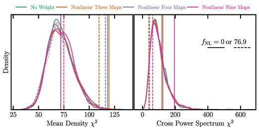
The remaining systematic error χ2 from the mean galaxy density contrast (left) and the galaxy-imaging normalized cross power spectrum (right). The values observed in the DESI LRG targets after the non-linear treatments are represented via vertical lines using the fNL = 0 (solid) or 76.9 (dashed) covariance, and the histograms are constructed from 1000 realizations of clean lognormal mocks with fNL = 0 (solid) and 76.9 (dashed).
Mean galaxy density contrast χ2 and normalized cross power spectrum χ2 from the DESI LRG targets and p-values that are inferred from the comparison to the fNL = 0 and 76.9 clean mocks that have received the same mitigation. For the case of No weight, we use the clean mocks without mitigation.
| Mean density contrast (dof = 72) | Cross power spectrum (dof = 81) | |||||||
|---|---|---|---|---|---|---|---|---|
| Covariance: fNL = 0 | fNL = 76.9 | fNL = 0 | fNL = 76.9 | |||||
| Method | χ2 | p-value | χ2 | p-value | χ2 | p-value | χ2 | p-value |
| No weight | 679.8 | < 0.001 | 405.2 | < 0.001 | 20014.8 | < 0.001 | 721.1 | < 0.001 |
| Non-linear three maps | 119.5 | 0.002 | 109.7 | 0.003 | 118.6 | 0.273 | 38.0 | 0.951 |
| Non-linear four maps | 118.2 | 0.001 | 115.9 | 0.001 | 124.6 | 0.240 | 43.3 | 0.921 |
| Non-linear nine maps | 71.9 | 0.487 | 74.9 | 0.392 | 195.1 | 0.047 | 62.2 | 0.767 |
The tests conducted here demonstrate the effectiveness of various cleaning approaches for the DESI LRG targets without revealing the measured power spectrum or fNL constraints. Overall, we observe that the non-linear method with the set of nine imaging property maps, successfully passes the mean density test irrespective of the covariance, as indicated by χ2 = 71.9 (p-value = >0.48) for the fNL = 0 covariance. On the other hand, the non-linear three maps and non-linear four maps methods both fail to sufficiently mitigate systematics in the mean density test, as evidenced by low p-values. Our work shows that it is essential to maintain a consistent covariance matrix, involving the same mitigation and ensuring consistency in fNL within the covariance. The sensitivity of the mean density χ2 to the fNL assumption in the covariance is notably lower, with greater reliance on the consistent mitigation method. Conversely, the normalized cross spectrum χ2 exhibits a higher dependency on the fNL assumption in the covariance. The mean density diagnostic appears to be a less cosmology-sensitive probe of residual systematics. As a robustness test, we also increase the largest ℓ used in the χ2 calculation to ℓ = 100, which corresponds to density fluctuations on angles smaller than 2°. But we find no remaining systematic error from higher harmonic modes (see Appendix A1). The conclusion of these tests is that the non-linear method with the set of nine maps passes our null tests for the remaining systematics, and thus is chosen as the default approach for the treatment of imaging systematic effects. In the following subsection, we show how imaging systematic regressions remove clustering modes, with increasing dependence on the number of maps used, and thus bias the best-fitting estimates of fNL. Then, we present how we calibrate for the overcorrection for our default mitigation method.
3.5 Calibration of overcorrection
The template-based mitigation of imaging systematics removes some of the true clustering signal, and mitigating with more maps should remove more modes and thus bias both the fNL estimation and its associated uncertainty. We calibrate the overcorrection effect using the mocks presented in Section 2. Having two sets of mocks with low and high power at large scales (low ℓ) offers a key advantage: it provides a model for mapping the entire posterior distribution, which enables us to understand how the constraints on fNL degrade as the magnitude of the imaging systematic correction increases. We apply the neural network model to both the fNL = 0 and 76.9 simulations, with and without imaging systematics, using various sets of imaging systematic maps. Specifically, we consider non-linear three maps, non-linear four maps, and non-linear nine maps. Then, we measure the power spectra from the mocks. We fit both the mean power spectrum and each individual power spectrum from the mocks. Appendix B2 outlines the impact of the non-linear methods on the mock power spectra, and here we summarize relevant details for the calibration of overcorrection.
Fig. 10 displays a comparison between the best-fitting estimates of fNL before and after mitigation for the clean mocks. The best-fitting estimates from the mean of the mocks are represented by the solid curves, and the individual spectra results are displayed as the scatter points. The results from fitting the mean power spectrum of the contaminated mocks are also shown via the dashed curves. We find nearly identical results for the biases caused by mitigation, whether or not the mocks have any contamination, which can be seen by observing the solid and dashed curves displayed on Fig. 10 (see also Fig. B4, for a comparison of the mean power spectrum). For clarity, the best-fitting estimates for the individual contaminated data are not shown in the figure.
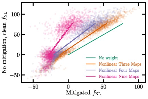
The No mitigated, clean versus mitigated fNL values from the fNL = 0 and 76.9 mocks. The solid (dashed) lines represent the best-fitting estimates from fitting the mean power spectrum of the clean (contaminated) mocks. The scatter points show the best-fitting estimates from fitting the individual spectra for the clean mocks.
As summarized in Table B2, we observe notable shifts in the best-fitting estimates of fNL obtained from the mean power spectrum of the mocks. Specifically, for the fNL = 0 mocks, we obtain ΔfNL = −12 for non-linear three maps, −20 for non-linear four maps, and −27 for non-linear nine maps. Larger shifts are evident for fNL = 76.9: ΔfNL = −23 for non-linear three maps, −39 for non-linear four maps, and −72 for non-linear nine maps. These factor imply that the effect of systematic mitigation on the inferred fNL depends on the true value of fNL.
To calibrate our methods, we fit a linear curve to the fNL estimates from the mean power spectrum of the mocks, fNL, no mitigation, clean = m1fNL, mitigated + m2. The m1 and m2 coefficients for non-linear three, four, and nine maps are summarized in Table 4. These coefficients represent the impact of the cleaning methods on the likelihood. The uncertainty in fNL after mitigation increases by m1 − 1. Fig. 10 also shows that the choice of our cleaning method can have significant implications for the accuracy of the measured fNL, and careful consideration should be given to the selection of the primary imaging systematic maps and the calibration of the cleaning algorithms in order to minimize systematic uncertainties.
Linear parameters employed to de-bias the fNL constraints to account for the overcorrection issue.
| Cleaning method | m1 | m2 |
|---|---|---|
| Non-linear three maps | 1.17 | 13.95 |
| Non-linear four maps | 1.32 | 26.97 |
| Non-linear nine maps | 2.35 | 63.5 |
| Cleaning method | m1 | m2 |
|---|---|---|
| Non-linear three maps | 1.17 | 13.95 |
| Non-linear four maps | 1.32 | 26.97 |
| Non-linear nine maps | 2.35 | 63.5 |
4 RESULTS
We now present our fNL constraints obtained from the power spectrum of the DESI LRG targets. The treatment of the imaging systematic effects is performed on each imaging region (BASS + MzLS, DECaLS North/South) separately. After cleaning, the regions are combined for the measurement of the power spectrum. We unblind the galaxy power spectrum and the fNL values after our cleaning methods are validated and vetted by the cross power spectrum and mean galaxy density diagnostics. As presented in Section 3.4, these tests show that none of the linear methods yields reasonable statistics, and only the non-linear approach with the nine maps can pass the criteria, which is why we select the non-linear nine maps as our fiducial method for cleaning systematics. We also conduct additional tests to check the robustness of our constraints against various assumptions, such as analysing each region separately, applying cuts on imaging conditions, and changing the smallest mode used in fitting for fNL.
4.1 DESI imaging LRG sample
We find that the excess clustering signal in the power spectrum of the DESI LRG targets is mitigated after correcting for the imaging systematic effects. Fig. 11 shows the measured power spectrum of the DESI LRG targets before and after applying imaging weights and the best-fitting theory curves. The solid grey line and the grey shade represent, respectively, the mean power spectrum and 1σ error, estimated from the fNL = 0 lognormal simulations. The differences between various cleaning methods are significant on large scales (ℓ < 20), but the small-scale clustering measurements are consistent. We associate the differences to the overcorrection caused by including more maps for the treatment of systematics, which we base upon the validation of the methods on the mocks, or the suppression of excess power from systematics. Comparing non-linear three maps to non-linear four maps, we find that adding stellar density in the non-linear approach (non-linear four maps) further reduces the excess power relative to the mock power spectrum, in particular on modes between 2 ≤ ℓ < 4. However, when calibrated on the lognormal simulations, we find that the oversubtraction due to stellar density is reversed after accounting for overcorrection. Our fiducial approach, non-linear nine maps, yields the lowest (and almost constant) power on large scales among all methods.
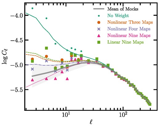
The angular power spectrum of the DESI LRG targets before (No weight) and after correcting for imaging systematics using the linear and non-linear methods. The curves represent the corresponding best-fitting theory predictions. The solid curve and grey shade, respectively, represent the mean power spectrum and |$68{{\ \rm per\ cent}}$| error from the fNL = 0 mocks.
4.1.1 Calibrated constraints
All fNL constraints presented here are calibrated for the effect of overcorrection using the lognormal simulations. Table 5 describes the best-fitting and marginalized mean estimates of fNL from fitting the power spectrum of the DESI LRG targets before and after cleaning with the non-linear approach given various combinations for the imaging systematic maps. Fig. 12 shows the marginalized probability distribution for fNL in the top panel, and the |$68{{\ \rm per\ cent}}$| and |$95{{\ \rm per\ cent}}$| probability contours for the linear bias parameter and fNL in the bottom panel, from our sample before and after applying various corrections for imaging systematics. Overall, we find the maximum-likelihood estimates to be consistent among the various cleaning methods. We obtain 33(21) < fNL < 61(76) at |$68{{\ \rm per\ cent}}(95{{\ \rm per\ cent}})$| confidence with χ2 = 33.9 for non-linear three maps with 34 degrees of freedom. Accounted for overcorrection, we obtain 33(19) < fNL < 62(78) with χ2 = 34.4 using non-linear four maps which includes the additional stellar density map. With or without stellar density, the confidence intervals are consistent with each other and significantly off from zero PNG; specifically, the probability that fNL is erroneously greater than zero, P(fNL > 0) = 99.9 per cent, which we attribute to systematics (see Section 3.4). We also apply a more aggressive systematics treatment that includes regression using the non-linear approach against the set of nine imaging maps we identified, non-linear nine maps, and find that zero fNL is recovered. Specifically, our maximum-likelihood value changes to fNL ∼ 34 with χ2 = 39.1, and the uncertainty on fNL increases by more than a factor of two, resulting in −10(− 39) < fNL < 58(84) at |$68{{\ \rm per\ cent}} (95{{\ \rm per\ cent}})$| confidence. This increase is attributed to the aggressive treatment, which removes large-scale clustering information and diminishes the constraining power of the data set.
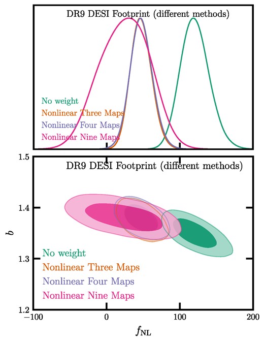
The calibrated constrains from the DESI LRG targets. Top: probability distribution for fNL marginalized over the shotnoise and bias. Bottom: |$68{{\ \rm per\ cent}}$| and |$95{{\ \rm per\ cent}}$| probability distribution contours for the bias and fNL from the DESI LRG targets before and after applying the non-linear cleaning methods. The lognormal mocks are used to calibrate these distributions for overcorrection.
The calibrated best-fitting, marginalized mean, and marginalized |$68\,\mathrm{ per\,cent}$| (|$95\,\mathrm{ per\,cent}$|) confidence estimates for fNL from fitting the power spectrum of the DESI LRG targets before and after correcting for imaging systematic effects. The lowest mode is ℓmin = 2, p = 1, and s = 0.945.
| fNL | ||||||
|---|---|---|---|---|---|---|
| Footprint | Method | Best fit | Mean | |$68\,\mathrm{ per\,cent}$| CL | |$95\,\mathrm{ per\,cent}$| CL | χ2 (dof = 34) |
| DESI | No weight | 118 | 121 | 102 < fNL < 140 | 86 < fNL < 161 | 45.1 |
| DESI | Non-linear three maps | 46 | 47 | 33 < fNL < 61 | 21 < fNL < 76 | 33.9 |
| DESI | Non-linear four maps | 46 | 47 | 33 < fNL < 62 | 19 < fNL < 78 | 34.4 |
| DESI | Non-linear nine maps | 34 | 24 | −10 < fNL < 58 | −39 < fNL < 84 | 39.1 |
Additionally, we explore the sensitivity of the fNL posterior using the non-linear nine maps method while varying the values of p in the range of 0.5 to 1.6 and s in the range of 0.75 to 1.25. Fig. 13 illustrates our findings, and Table 6 provides a summary. Regardless of the specific values chosen for p and s, we reliably recover fNL = 0 within the |$95{{\ \rm per\ cent}}$| confidence interval. The top panel also implies that marginalizing over p can induce projection effects and lead to biased fNL constraints. For comparison, we obtain 102(86) < fNL < 140(161) at |$68{{\ \rm per\ cent}} (95{{\ \rm per\ cent}})$| confidence with χ2 = 45.1 for the no weight case.
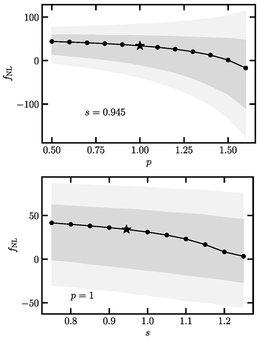
The best-fitting estimates of fNL and their corresponding |$68{{\ \rm per\ cent}}$| (|$95{{\ \rm per\ cent}}$|) errors from the DESI LRG targets using the non-linear nine maps approach given various values of p or s. The star symbol represents the fiducial analysis with p = 1 and s = 0.945.
The calibrated best-fitting, marginalized mean, and marginalized |$68\,\mathrm{ per\,cent}$| (|$95\,\mathrm{ per\,cent}$|) confidence estimates for fNL from the DESI LRG targets cleaned with the non-linear nine maps approach, given various values of p and s. The fiducial analysis uses p = 1 and s = 0.945 (DESI footprint).
| fNL | |||||
|---|---|---|---|---|---|
| Parameter | Best fit | Mean | |$68\,\mathrm{ per\,cent}$| CL | |$95\,\mathrm{ per\,cent}$| CL | χ2 (dof = 34) |
| p = 0.5 | 44 | 37 | 14 < fNL < 60 | −6 < fNL < 77 | 39.1 |
| 0.6 | 43 | 35 | 11 < fNL < 59 | −11 < fNL < 78 | 39.1 |
| 0.7 | 41 | 33 | 7 < fNL < 59 | −16 < fNL < 80 | 39.1 |
| 0.8 | 39 | 31 | 2 < fNL < 58 | −22 < fNL < 80 | 39.1 |
| 0.9 | 37 | 28 | −3 < fNL < 58 | −30 < fNL < 82 | 39.1 |
| 1.0 | 34 | 24 | −10 < fNL < 58 | −39 < fNL < 84 | 39.1 |
| 1.1 | 31 | 19 | −18 < fNL < 57 | −50 < fNL < 86 | 39.1 |
| 1.2 | 26 | 15 | −28 < fNL < 56 | −64 < fNL < 89 | 39.1 |
| 1.3 | 21 | 7 | −41 < fNL < 54 | −80 < fNL < 93 | 39.0 |
| 1.4 | 13 | −2 | −58 < fNL < 53 | −103 < fNL < 97 | 39.0 |
| 1.5 | 1 | −13 | −77 < fNL < 51 | −131 < fNL < 104 | 39.0 |
| 1.6 | −17 | −31 | −110 < fNL < 47 | −175 < fNL < 114 | 39.0 |
| s = 0.75 | 42 | 31 | −1 < fNL < 62 | −30 < fNL < 87 | 39.2 |
| 0.80 | 40 | 30 | −3 < fNL < 61 | −32 < fNL < 86 | 39.1 |
| 0.85 | 38 | 28 | −6 < fNL < 60 | −35 < fNL < 86 | 39.1 |
| 0.90 | 36 | 26 | −8 < fNL < 58 | −36 < fNL < 84 | 39.1 |
| 0.945 | 34 | 24 | −10 < fNL < 58 | −39 < fNL < 84 | 39.1 |
| 1.00 | 31 | 22 | −13 < fNL < 56 | −42 < fNL < 83 | 39.0 |
| 1.05 | 28 | 19 | −15 < fNL < 54 | −45 < fNL < 81 | 39.0 |
| 1.10 | 23 | 17 | −18 < fNL < 52 | −48 < fNL < 80 | 39.0 |
| 1.15 | 17 | 15 | −21 < fNL < 51 | −50 < fNL < 80 | 38.9 |
| 1.20 | 8 | 12 | −24 < fNL < 48 | −53 < fNL < 77 | 38.9 |
| 1.25 | 3 | 9 | −27 < fNL < 46 | −56 < fNL < 76 | 38.8 |
4.1.2 Uncalibrated constraints: robustness tests
Fig. 14 shows the probability distributions of fNL for various treatments before accounting for the overcorrection effect. The method with the largest flexibility and more number of imaging systematic maps is more likely to regress out the clustering signal aggressively and return biased fNL constraints. The non-linear three maps approach returns a best-fitting estimate of fNL = 27 with the |$68{{\ \rm per\ cent}}(95{{\ \rm per\ cent}})$| confidence of 17(6) < fNL < 40(53) and χ2 = 33.9. With the stellar density map included, non-linear four maps yields a smaller best-fitting estimates of fNL = 14 with the error of 5(− 6) < fNL < 26(38). The non-linear nine maps gives an asymmetric posterior with the marginalized mean fNL = −17, and the smallest best-fitting estimate of fNL = −13 with the error of −31(− 44) < fNL < −3(9). The disparities in the best-fitting estimates can be linked to overcorrection, mirroring the effects observed in the mocks (refer to Fig. B5). Consequently, caution is advised when considering the uncalibrated values. Without adjusting for overcorrection, non-linear four maps and non-linear nine maps recover zero fNL within |$95{{\ \rm per\ cent}}$| and |$68{{\ \rm per\ cent}}$| confidence, respectively. However, the non-linear method with three maps exhibits tension with fNL = 0 at a confidence level of 99.5 per cent.
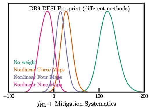
Same as Fig. 12, but without accounting for overcorrection.
Now we proceed to perform some robustness tests and assess how sensitive the fNL constraints are to the assumptions made in the analysis or the quality cuts applied to the data. For each case, we retrain the cleaning methods and derive new sets of imaging weights. Accordingly, for the cases where a new survey mask is applied to the data, we recalculate the covariance matrices using the new survey mask to account for the changes in the survey window and integral constraint effects. Calibrating the mitigation biases for all of these experiments is beyond the scope of this work and redundant, as we are only interested in the relative shift in the fNL constraints after changing the assumptions. Therefore, the absolute scaling of the fNL constraints presented here are biased because of the overcorrection effect. Table 7 summarizes the uncalibrated fNL constraints from the DESI LRG targets. Our tests are as follows:
The uncalibrated best-fitting and marginalized mean estimates for fNL from fitting the power spectrum of the DESI LRG targets before and after correcting for systematics. The estimates are not calibrated for overcorrection, and thus are subject to mitigation systematics. The number of degrees of freedom is 34 (37 data points − 3 parameters) for all cases except the case that combines the data at the likelihood level, ‘BASS+MzLS + DECaLS’, in which the dof is 104 (3 × 37 − 7). The lowest mode is ℓ = 2 and the covariance matrix is from the fNL = 0 clean mocks (no mitigation) except for the case with ‘ + Cov’ in which the covariance matrix is from the fNL = 76.9 clean mocks (no mitigation). We fix p = 1 for all cases and s = 0.945 for DESI, 0.943 for DECaLS North (and South), and 0.951 for BASS + MzLS. The bold values represent important cases.
| fNL + Mitigation systematics | ||||||
|---|---|---|---|---|---|---|
| Footprint | Method | Best fit | Mean | |$68\,\mathrm{ per\,cent}$| CL | |$95\,\mathrm{ per\,cent}$| CL | χ2 (dof = 34) |
| DESI | No weight | 118 | 121 | 102 < fNL < 140 | 86 < fNL < 161 | 45.1 |
| DESI | Linear three maps | 36 | 37 | 25 < fNL < 50 | 14 < fNL < 64 | 38.6 |
| DESI | Linear four maps | 31 | 32 | 20 < fNL < 45 | 9 < fNL < 58 | 40.3 |
| DESI | Linear nine maps | 30 | 32 | 19 < fNL < 43 | 9 < fNL < 57 | 41.9 |
| DESI | Non-linear three maps | 27 | 28 | 17 < fNL < 40 | 6 < fNL < 53 | 33.9 |
| DESI | Non-linear four maps | 14 | 15 | 5 < fNL < 26 | −6 < fNL < 38 | 34.4 |
| DESI | Non-linear nine maps | − 13 | − 17 | − 31 < fNL < − 3 | − 44 < fNL < 9 | 39.1 |
| DESI (imag. cut) | Non-linear nine maps | −25 | −22 | −37 < fNL < −7 | −49 < fNL < 6 | 37.7 |
| DESI (comp. cut) | Non-linear nine maps | −24 | −23 | −35 < fNL < −10 | −46 < fNL < 2 | 36.3 |
| DESI | Non-linear nine maps + fNL = 76.9 Cov | −11 | −15 | −30 < fNL < 0 | −43 < fNL < 12 | 37.4 |
| BASS+MzLS + DECaLS | Non-linear nine maps | −31 | −26 | −41 < fNL < −9 | −53 < fNL < 5 | 114.2 |
| BASS + MzLS | Non-linear three maps | 13 | 16 | −6 < fNL < 38 | −28 < fNL < 64 | 34.9 |
| BASS + MzLS | Non-linear four maps | 10 | 12 | −11 < fNL < 34 | −35 < fNL < 59 | 34.1 |
| BASS + MzLS | Non-linear nine maps | − 9 | − 13 | − 37 < fNL < 10 | − 59 < fNL < 32 | 36.4 |
| BASS + MzLS (imag. cut) | Non-linear nine maps | −12 | −13 | −36 < fNL < 10 | −58 < fNL < 34 | 36.7 |
| BASS + MzLS (comp. cut) | Non-linear nine maps | −15 | −16 | −39 < fNL < 6 | −61 < fNL < 28 | 35.3 |
| DECaLS North | Non-linear three maps | 41 | 45 | 21 < fNL < 69 | −1 < fNL < 98 | 40.8 |
| DECaLS North | Non-linear four maps | 30 | 32 | 10 < fNL < 56 | −18 < fNL < 83 | 40.9 |
| DECaLS North | Non-linear nine maps | − 4 | − 13 | − 40 < fNL < 13 | − 64 < fNL < 36 | 44.6 |
| DECaLS North (imag. cut) | Non-linear nine maps | −16 | −20 | −47 < fNL < 7 | −70 < fNL < 31 | 36.1 |
| DECaLS North (comp. cut) | Non-linear nine maps | −17 | −20 | −46 < fNL < 5 | −68 < fNL < 28 | 42.7 |
| DECaLS North (no Dec. cut) | Non-linear nine maps | 0 | −13 | −43 < fNL < 15 | −67 < fNL < 38 | 44.2 |
| DECaLS North | Non-linear eleven maps | −2 | −7 | −32 < fNL < 16 | −54 < fNL < 39 | 40.0 |
| DECaLS South | Non-linear three maps | 30 | 31 | 11 < fNL < 53 | −28 < fNL < 76 | 30.2 |
| DECaLS South | Non-linear four maps | −42 | −5 | −44 < fNL < 27 | −70 < fNL < 49 | 33.4 |
| DECaLS South | Non-linear nine maps | − 43 | − 40 | − 58 < fNL < − 21 | − 75 < fNL < 3 | 31.3 |
| DECaLS South (imag. cut) | Non-linear nine maps | −57 | −55 | −76 < fNL < −36 | −96 < fNL < −8 | 30.0 |
| DECaLS South (comp. cut) | Non-linear nine maps | −42 | −40 | −58 < fNL < −22 | −76 < fNL < −1 | 30.4 |
| DECaLS South (no Dec. cut) | Non-linear nine maps | −2 | −10 | −31 < fNL < 10 | −50 < fNL < 26 | 26.1 |
| DECaLS South | Non-linear eleven maps | −38 | −35 | −52 < fNL < −16 | −70 < fNL < 5 | 32.3 |
Linear methods: even though the linear methods show remaining systematics (e.g. against depth in z as shown in Fig. 8), we obtain identical constraints from linear four and nine maps, respectively, 20(9) < fNL < 45(58) and 19(9) < fNL < 43(57) at |$68{{\ \rm per\ cent}}(95{{\ \rm per\ cent}})$| confidence. For the linear treatment methods, the probability of fNL being greater than zero is erroneously 99.9 per cent. Any attempt to account for the overcorrection would elevate this probability even further. The overestimation of fNL can be attributed to an increase in systematic contamination.
Imaging regions: we compare how our constraints from fitting the power spectrum of the whole DESI footprint compares to that from the power spectrum of each imaging region individually, namely BASS + MzLS, DECaLS North, and DECaLS South. Fig. 15 shows the |$68{{\ \rm per\ cent}}$| and |$95{{\ \rm per\ cent}}$| probability contours on fNL and b from each individual region, compared with that from DESI. The cleaning method here is non-linear nine maps, and the covariance matrices are estimated from the fNL = 0 mocks. The bias in DECaLS North is lower than the ones from DECaLS South and BASS + MzLS, which might indicate some remaining systematic effects that could not be mitigated with the available imaging systematic maps. This is because given the negative correlation between b and fNL, a larger value of fNL due to excess clustering power needs to be compensated by a smaller value of b. Overall, we find that the constraints from analysing each imaging survey separately are consistent with each other and DESI within |$68{{\ \rm per\ cent}}$| confidence. We also consider combining the data at the likelihood level (‘BASS+MzLS + DECaLS’). In this case, the total number of data points is 111 (3 × 37). We allow the bias and shotnoise parameters to vary independently for each subregion but use a single and common fNL value, which brings the total number of free parameters to 7 and the number of degrees of freedom to 104. We obtain a best-fitting estimate of fNL = −31 with χ2 = 114.2 and |$68{{\ \rm per\ cent}}$| (|$95{{\ \rm per\ cent}}$|) confidence interval of −41(− 53) < fNL < 9(5). Compared with our fiducial analysis which combines the data at the map level, we observe around |$13{{\ \rm per\ cent}}$| loss in constraining power.
Stellar density template ( nStar ): when not accounting for overcorrection, adding the stellar density map appears to result in significant changes in the fNL constraints, for example, compare non-linear three maps with non-linear four maps in Table 7. But these changes disappear when we account for the mitigation bias and we find both methods recover the same maximum-likelihood estimate for fNL ∼ 46 within |$69{{\ \rm per\ cent}}$| confidence, see Table 5, which implies that these changes can be associated with the overcorrection issue from the chance correlations between the stellar density map and LSS.
Pixel completeness ( comp. cut): we discard pixels with fractional completeness less than half to assess the effect of partially complete pixels on fNL. This pixel completeness cut removes |$0.6{{\ \rm per\ cent}}$| of the survey area, and no significant changes in the fNL constraints are observed.
Imaging quality ( imag. cut ): pixels with poor photometry are removed from our sample by applying the following cuts on imaging; E[B − V] < 0.1, nStar < 3000, depthg > 23.2, depthr > 22.6, depthz > 22.5, psfsizeg < 2.5, psfsizer < 2.5, and psfsizez < 2. Although these cuts remove |$8{{\ \rm per\ cent}}$| of the survey mask, there is a negligible impact on the best-fitting estimates of fNL from fitting the DESI power spectrum. However, when each region is fit individually, the BASS + MzLS constraint is more stable than those from DECaLS North and DECaLS South.
Covariance matrix ( cov): we fit the power spectrum of our sample cleaned with non-linear nine maps, but use the covariance matrix constructed from the fNL = 76.9 mocks. With the alternative covariance, a |$7{{\ \rm per\ cent}}$| increase in the 68 per cent error on fNL, σ(fNL), is observed. We also find that the best-fitting and marginalized mean estimates of fNL increase slightly by ΔfNL = 2. Overall, we find that the differences are not significant in comparison to the statistical precision.
External maps ( CALIBZ + H i ): the neural network eleven maps correction includes the additional maps for the neutral column density (H i) and the z-band calibration error (CALIBZ). With this correction, the best-fitting fNL increases from −4 to −2 for DECaLS North and from −43 to −38 for DECaLS South, which might suggest that adding H i and CALIBZ increases the input noise, and thus negatively impacts the performance of the neural network model. This test is not performed on BASS + MzLS due to a lack of coverage from the CALIBZ map.
Declination mask ( no DEC cut ): the fiducial mask removes the disconnected islands in DECaLS North and regions with Dec. <−30 in DECaLS South, where there is a high likelihood of calibration issues as different standard stars are used for photometric calibrations. We analyse our sample without these cuts, and find that the best-fitting and marginalized fNL mean estimates from DECaLS South shift significantly to higher values of fNL by ΔfNL ∼ 41, which supports the case that there are remaining photometric systematics in the DECaLS South region below Dec. =−30. On the other hand, the constraints from DECaLS North do not change significantly, indicating the islands do not induce significant contaminations.
Scale dependence ( varying ℓmin ): we raise the value of the lowest harmonic mode ℓmin used for the likelihood evaluation during MCMC. This is equivalent to utilizing smaller spatial scales in the measurements of the power spectrum. By doing so, we anticipate a reduction in the impact of imaging systematics on fNL inference as lower ℓ modes are more likely to be contaminated. Fig. 16 illustrates the power spectra before and after the correction with non-linear nine maps in the top panel. The bottom panel shows the best-fitting estimate and |$95{{\ \rm per\ cent}}$| error on fNL with non-linear nine maps for the DESI, BASS + MzLS, DECaLS North, and DECaLS South regions. We discover that a slight upward shift in the best-fitting estimates of fNL on scales ranging from 10 to 20 for DECaLS North and BASS + MzLS when we utilized a higher ℓmin. This outcome might imply that the imaging systematic maps do not contain enough information to help the cleaning method null out the contaminating signal in the NGC. We also find that the bump is resilient against an alternative correction, in which we apply the neural networks trained on the DECaLS South to the DECaLS North region (see Appendix A4). Overall, this result is contrary to what one might predict if a significant systematic-induced spike existed at the very low ℓ, or if we had an extremely large-scale systematic leakage from the ℓ = 1 mode. As a result, it suggests that the underlying issue is more subtle than originally anticipated.
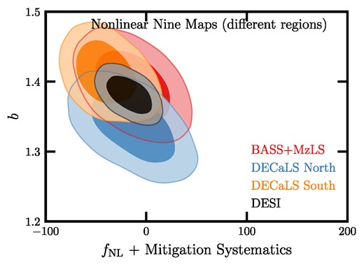
The uncalibrated 2D constraints from the DESI LRG targets using the non-linear nine maps treatment for each imaging survey compared with that for the whole DESI footprint. The dark and light shades represent the |$68{{\ \rm per\ cent}}$| and |$95{{\ \rm per\ cent}}$| confidence intervals, respectively.
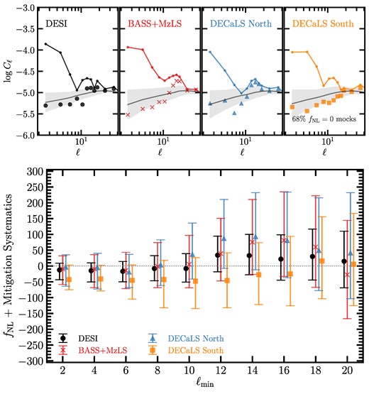
Top: the measured power spectrum of the DESI LRG targets before (solid curves) and after non-linear nine maps (scatter points) for the DESI, BASS + MzLS, DECaLS North, and DECaLS South regions. The solid curve and grey shade, respectively, represent the mean power spectrum and |$68{{\ \rm per\ cent}}$| error from the fNL = 0 mocks with the same angular mask for each region. Bottom: the uncalibrated fNL constraints versus the lowest ℓ mode used for fitting fNL. The points represent the best-fitting estimates of fNL and error bars represent 95 per cent confidence. The scaling of fNL is not calibrated to account for overcorrection caused by mitigation.
5 DISCUSSION AND CONCLUSION
We have measured the local PNG parameter fNL using the scale-dependent bias in the angular clustering of LRGs selected from the DESI Legacy Imaging Survey DR9. Our sample includes more than 12 million LRG targets covering around |$14\, 000$| deg2 in the redshift range of 0.2 < z < 1.35. We leverage early spectroscopy during DESI SV (DESI Collaboration 2024) to infer the redshift distribution of our sample (Fig. 1). Our power spectrum model accounts for various theoretical and observational effects such as RSD, magnification bias, survey geometry, and integral constraint. Most importantly, we utilize a novel machine-learning method to mitigate the effect of imaging systematics and reduce excess clustering power on large scales (or low ℓ). We use lognormal simulations to estimate the covariance matrices. As a caveat, this omits the contributions from higher order statistics in the covariance matrix, but we leave that for future as we do not anticipate any major impact on the best-fitting estimates of fNL.
In our fiducial analysis, which includes a non-linear treatment of systematics using nine imaging property maps (Galactic extinction, stellar density, depth in grzW1, and psfsize in grz), we obtain |$f_{\rm NL} = 34^{+24(+50)}_{-44(-73)}$| with p = 1 and s = 0.945. This measurement is consistent with recent CMB and LSS measurements, as visualized in Fig. 17. The sensitivity of our constraints is explored against p and s. The best-fitting estimates of fNL decrease as we increase either p or s. Specifically, we find that the error on fNL is more sensitive to p than s. Compared with the fiducial result, the error increases by more than a factor of two for p = 1.6, and only by |$7{{\ \rm per\ cent}}$| for s = 1.25 (Fig. 13). The minimum χ2 however does not change much, indicating that the impact on the power spectrum fit is negligible.
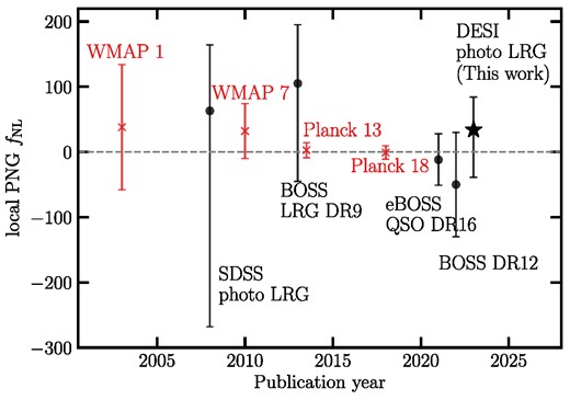
History of constraints on local PNG fNL at |$95{{\ \rm per\ cent}}$| confidence from single-tracer LSS (Slosar et al. 2008; Ross et al. 2013; Mueller et al. 2022; Cabass et al. 2022), including our analysis with −39 < fNL < 84 (DESI photo LRG) and CMB surveys (Komatsu et al. 2003; Komatsu 2010; Planck Collaboration XXIV 2014; Planck Collaboration IX 2020). The median fNL value is used in case the maximum-likelihood estimate was not reported in the reference.
The signature of local PNG is very sensitive to excess clustering power caused by imaging systematic effects. We have applied a series of robustness tests to investigate the impact of how the galaxy selection function is determined. Specifically, both linear and non-linear methods are applied using various combinations of imaging systematic maps (including two external maps for the neutral hydrogen column density and photometric calibration error in the z band). We also examine the effect of additional masks based on imaging conditions and survey completeness. Overall, we find that no change in the analysis shifts the maximum-likelihood value of fNL to a significantly different value (Figs 15 and 16, and Table 7).
Although being essential for the mitigation of imaging systematics, the template-based approach inevitably removes some of the large-scale clustering information. One of the primary highlights of this work is that we present a strategy to calibrate the systematic mitigation’s impact on the inferred fNL. As we increase the number of maps for mitigation, more of the power spectrum is removed, introducing a larger bias to the fNL posterior distribution. Our mock tests suggest that this bias is fNL-dependent, such that the mocks with larger fNL experience a more substantial reduction in the low-ℓ power due to systematic mitigation. Therefore, it is crucial to calibrate for this effect using simulations that have gone through the same treatment methods and are subject to the same overcorrection effect.
As a greater flexibility in the mitigation increases the overcorrection and decreases the statistical power, we tested if we can reduce the flexibility in our method by using a smaller set of maps, including Galactic extinction, depth in the z band, and astronomical seeing in the r band (non-linear three maps) to retain some constraining power. Additionally, we consider an additional map for local stellar density (non-linear four maps). Using three or four maps, we can qualitatively mitigate systematic trends in the mean galaxy density and cross-correlations of the galaxy density field and imaging property maps (see Section 3.4). These methods do not degrade the error on fNL as much as the fiducial method which used nine maps. However, when applying our null tests that are applied in order to detect residual systematic variance (see Section 3.4), we obtain passing results only for the non-linear nine map case. In this work, we found updating the covariance matrix for each particular variation (e.g. the mitigation method applied) was important in order to obtain a similar χ2 of the null test when applied to the mocks and hence self-consistently obtain a p-value for the null test. Another important conclusion from applying our null tests to mocks is that the mean density contrast test is less sensitive to the fNL value for the mocks than the angular cross-power. Given the amount of fNL constraining power that we lose when applying the nine map regression (the uncertainties approximately double), our findings highlight the importance of exploring, developing, and validating alternative mitigation approaches to avoid overcorrection for a robust analysis of local PNG.
Our analysis can be considered as the first attempt to identify major systematics in DESI, so we can be ready for constraining fNL with DESI spectroscopy. Internal DESI tests of the photometric calibration were unable to uncover DESI-specific issues, for example, when comparing to Gaia data. The most significant trends that we find are with the E(B−V) map. The source of such a trend would be a miscalibration of the E(B−V) map itself or the coefficients applied to obtain Galactic extinction corrected photometry. Such a miscalibration would plausibly be proportional in amplitude to the estimated E(B−V) map, though it may not have E(B−V)’s spatial distribution. There are ongoing efforts within DESI to obtain improved Galactic extinction information, which will help us address systematics. Additionally, cross-correlations of the DESI LRG density with the CMB lensing map is more stable in terms of systematics and can complement the results presented in this work. We can further avoid the overfitting issue by combining our neural network-based treatment method with forward-modelling techniques, such as Obiwon (Kong et al. 2020), but we will leave that for future work.
ACKNOWLEDGEMENTS
We would like to thank Douglas Finkbeiner for feedback on an early version of the manuscript; Violeta Gonzalez-Perez for handling the DESI internal review process; Tanveer Karim, Sukhdeep Singh, Ahmad Shamloumehr, and Reza Katebi for helpful discussions; and Rongpu Zhou for estimating the slope of the number counts and providing the maps for galaxy density and imaging systematics. MR would like to thank Ohio State’s Center for Cosmology and AstroParticle Physics, in particular, John Beacom and Lisa Colarosa, for their hospitality and support. MR is supported by the U.S. Department of Energy grants DE-SC0021165 and DE-SC0011840. H-JS acknowledges support from the U.S. Department of Energy, Office of Science, Office of High Energy Physics under grant nos DE-SC0019091 and DE-SC0023241. AP acknowledges support from the UK Science and Technology Facilities Council (STFC) under grant no. ST/V000594/1 and from the European Union’s Horizon Europe program under the Marie Sklodowska-Curie grant agreement 101068581. FB is a University Research Fellow, and has received funding from the European Research Council (ERC) under the European Union’s Horizon 2020 research and innovation program (grant agreement 853291). BB-K is supported by the project ᅮ주거대구조를 이용한 암흑우주 연구 (‘Understanding Dark Universe Using Large Scale Structure of the Universe’), funded by the Ministry of Science of the Republic of Korea. We acknowledge the support and resources from the Ohio Supercomputer Center (OSC; Center 1987). This research has made substantial use of the arXiv preprint server, NASA’s Astrophysics Data System, Github’s online software development platform, and many open-source software, such as pytorch, nbodykit, healpix, fitsio, scikit-learn, numpy, scipy, pandas, ipython, and jupyter.
This material is based upon work supported by the U.S. Department of Energy (DOE), Office of Science, Office of High-Energy Physics, under contract no. DE-AC02-05CH11231, and by the National Energy Research Scientific Computing Center, a DOE Office of Science User Facility under the same contract. Additional support for DESI was provided by the U.S. National Science Foundation (NSF), Division of Astronomical Sciences under contract no. AST-0950945 to the NSF’s National Optical-Infrared Astronomy Research Laboratory; the Science and Technology Facilities Council of the United Kingdom; the Gordon and Betty Moore Foundation; the Heising-Simons Foundation; the French Alternative Energies and Atomic Energy Commission (CEA); the National Council of Science and Technology of Mexico (CONACYT); the Ministry of Science and Innovation of Spain (MICINN), and by the DESI Member Institutions: https://www.desi.lbl.gov/collaborating-institutions.
The DESI Legacy Imaging Surveys consist of three individual and complementary projects: the DECaLS, the BASS, and the MzLS. DECaLS, BASS and MzLS together include data obtained, respectively, at the Blanco telescope, Cerro Tololo Inter-American Observatory, NSF’s NOIRLab; the Bok telescope, Steward Observatory, University of Arizona; and the Mayall telescope, Kitt Peak National Observatory, NOIRLab. NOIRLab is operated by the Association of Universities for Research in Astronomy (AURA) under a cooperative agreement with the National Science Foundation. Pipeline processing and analyses of the data were supported by NOIRLab and the Lawrence Berkeley National Laboratory. Legacy Surveys also uses data products from the Near-Earth Object Wide-field Infrared Survey Explorer (NEOWISE), a project of the Jet Propulsion Laboratory/California Institute of Technology, funded by the National Aeronautics and Space Administration. Legacy Surveys was supported by: the Director, Office of Science, Office of High Energy Physics of the U.S. Department of Energy; the National Energy Research Scientific Computing Center, a DOE Office of Science User Facility; the U.S. National Science Foundation, Division of Astronomical Sciences; the National Astronomical Observatories of China, the Chinese Academy of Sciences and the Chinese National Natural Science Foundation. LBNL is managed by the Regents of the University of California under contract to the U.S. Department of Energy. The complete acknowledgments can be found at https://www.legacysurvey.org/.
Any opinions, findings, and conclusions or recommendations expressed in this material are those of the author(s) and do not necessarily reflect the views of the U.S. National Science Foundation, the U.S. Department of Energy, or any of the listed funding agencies.
The authors are honoured to be permitted to conduct scientific research on Iolkam Du’ag (Kitt Peak), a mountain with particular significance to the Tohono O’odham Nation.
DATA AVAILABILITY
The DR9 catalogues from the DESI Legacy Imaging Surveys are publicly available at https://www.legacysurvey.org/dr9/. The software used for cleaning the imaging data is available at https://github.com/mehdirezaie/sysnetdev. All data points shown in the published graphs are available in a machine-readable form at https://zenodo.org/records/10594656.
Footnotes
See https://www.legacysurvey.org/dr9/bitmasks/ for maskbit definitions.
dN/dr = (dN/dz)(dz/dr) ∝ (dN/dz)H(z).
H0 = 100 (km s−1)/(h−1Mpc) and k is in unit of hMpc−1.
Dr. Rongpu Zhou (private communication).
REFERENCES
APPENDIX A: EXTRA ROBUSTNESS TESTS
A1 Scale-dependent systematics
To investigate the statistical significance of the cross power spectrum’s χ2, we examine its dependence on the largest harmonic mode ℓmax. Our fiducial cross power spectrum diagnostic (equation 19) uses harmonic modes up to ℓ = 20, which determines the smallest scale used for characterizing residual systematic errors. We extend ℓmax from 20 to 100, where the latter scale corresponds to density fluctuations on scales smaller than 2°. Fig. A1 shows the median of the normalized cross power spectrum’s χ2 from the clean fNL = 0 mocks after non-linear nine maps as the highest mode ℓmax increases from 20 to 100 (represented by the solid line). The pink circles represent the χ2 values for the DESI LRG targets cleaned with the non-linear nine maps method. Overall, we find that for all scales up to ℓ = 100, the non-linear nine maps approach yields consistent values with the clean mocks.
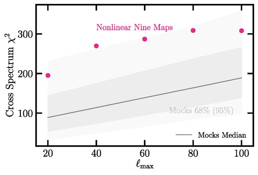
The cross power spectrum’s χ2 between the DESI LRG target density and imaging systematic maps as a function of the highest mode ℓmax when the sample is cleaned with the linear (triangles) and non-linear (squares) three maps. The lowest mode is fixed at ℓmin = 2. The solid curve and dark (light) shade represent the median value and |$68{{\ \rm per\ cent}}$| (|$95{{\ \rm per\ cent}}$|) confidence regions, estimated from the fNL = 0 mocks.
A2 Survey window convolution
Here, we calculate the mode–mode coupling matrix from the DESI mask. This matrix depends only on the survey geometry and can be described in terms of the window power spectrum (Hivon et al. 2002),
where the last term in the right-hand side represents the Wigner 3-j symbol (or Clebsch–Gordan coefficient), and is calculated using SymPy (Meurer et al. 2017). We benchmark our code against the publicly available software, NaMaster6 (Alonso et al. 2019). Fig. A2 illustrates various approaches to address the mode–mode coupling resulting from the DESI survey window at two arbitrary values of fNL. The red shade represents the 68 per cent dispersion of the fNL = 76.9 mocks. When fNL = 0, our config-space convolution of the window aligns with the ℓ-space convolution approach. However, when fNL = 76.9, both the config-space and NaMaster ℓ-space methods yield a convoluted power spectrum with noticeable noise-like numerical artefacts on large scales, therefore possibly in an fNL-dependent manner. To assess the impact of these discrepancies on our fNL constraints, we fit the clustering of the DESI LRG targets, disregarding the integral constraint effect. The best-fitting estimates of fNL will be biased, but our focus is on understanding the relative impact on fNL between the two approaches. For both config-space and ℓ-space methods, we obtain a similar minimum χ2 value of 39.6 with 34 degrees of freedom. Notably, the posterior width for the config-space approach is slightly larger than that of the ℓ-space by |$10{{\ \rm per\ cent}}$|. The absolute difference in the best-fitting estimates of fNL between the two cases is less than 1.1, considered negligible relative to the statistical precision of our measurements.
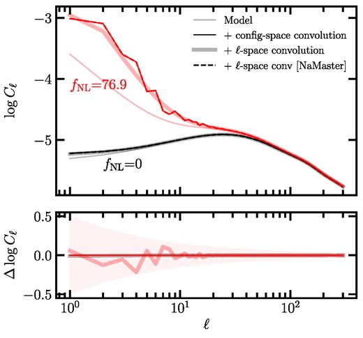
The model power spectrum before and after the survey geometry convolution for fNL = 0 and 76.9 using the DESI survey mask. The bottom panel shows the residual error with respect to the NaMaster code. The shade represents the dispersion of the fNL = 76.9 mocks.
A3 Redshift uncertainties
We use the Early Data Assembly Version 1 (EDA V1) to construct the redshift distribution for the DESI LRG targets. We find that the change in the maximum-likelihood estimate of fNL is negligible, |ΔfNL| < 1, compared to the statistical precision of our measurements. Fig. A3 shows the measured power spectrum of the DESI targets and the corresponding best-fitting theory curves. The variations in dN/dz do not significantly alter the conclusion of our paper.
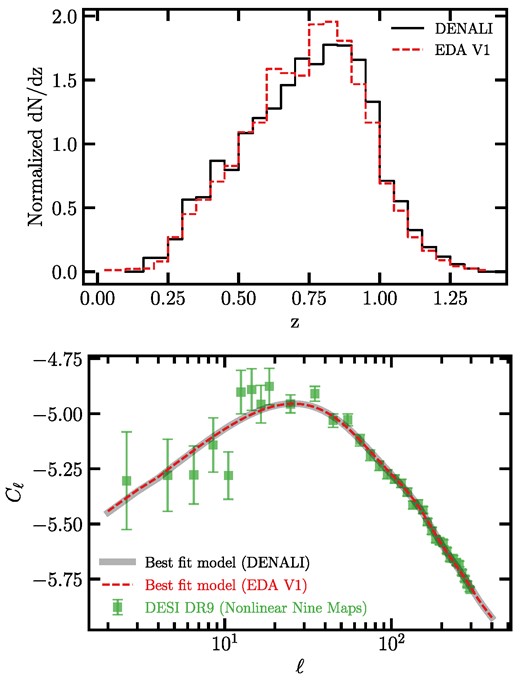
Top: the redshift distribution of the DESI LRG targets from the EDA V1 and Denali. Bottom: the measured power spectrum of the DESI LRG targets and the best-fitting theory models using different redshift distributions.
A4 Spurious bump in NGC
As shown in Fig. 16 (top panel), we realize that the spurious feature at ℓ ∼ 10–20 is removed in the DECaLS South region after mitigation, but it remains in the BASS + MzLS and DECaLS North. We use the neural networks trained on the DECaLS South with three and nine maps to mitigate the galaxy density in the DECaLS North region, and then measure the power spectrum. Fig. A4 shows the power spectrum before treatment (No weight) and after the non-linear three maps and nine maps methods for comparison. We find that whatever causing the bump is different between the DECaLS North and South. The best-fitting estimates for fNL from the DR9 DECaLS North using the neural network correction with three maps (NN trained on DECaLS North), three maps (NN trained on DECaLS South), and nine maps (NN trained on DECaLS South) are 41, 36, and 75, respectively. The solution without correction (No weight) results in a best-fitting estimate of fNL = 94.
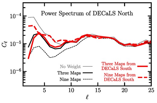
The unbinned measured power spectrum of the DESI LRG targets in the DECaLS North region before and after various mitigations using the neural network approach.
APPENDIX B: LOGNORMAL MOCKS
We fit the mean power spectrum of the lognormal mocks to validate the modelling pipeline, and in particular the survey geometry and integral constraint treatments. We investigate the impact of covariance matrix on the inference of fNL. Finally, we show the impact of imaging systematic mitigation and the oversubtraction effect when the cleaning methods are applied to the mocks.
B1 Clean mocks
The|$68{{\ \rm per\ cent}}$| and |$95{{\ \rm per\ cent}}$| probability contours on the PNG parameter fNL and bias coefficient b are shown in Figs B1 and B2, respectively, for the fNL = 0 and 76.9 mocks. The best-fitting, marginalized mean estimates, as well as the 1σ and 2σ confidence intervals of fNL are summarized in Table B1.
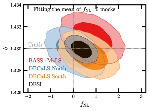
68 per cent and 95 per cent confidence contours from the mean power spectrum of the fNL = 0 mocks for the DESI footprint and subimaging surveys. The truth values are represented by vertical and horizontal lines.
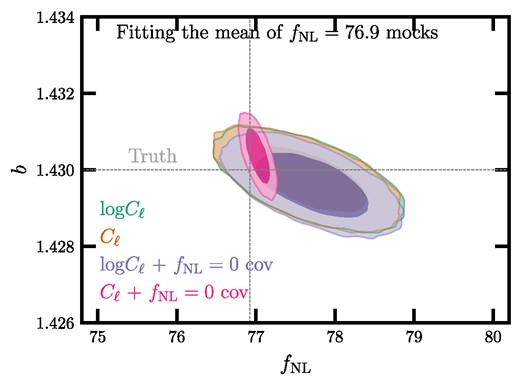
68 per cent and 95 per cent confidence contours of fitting the mean power spectrum or its log transformation from the fNL = 76.9 mocks for the DESI footprint. Using the log Cℓ fitting yield constraints that are insensitive to the covariance used. The truth values are represented by vertical and horizontal lines.
The best-fitting and marginalized mean estimates for fNL from fitting the mean power spectrum of the mocks. The covariance is scaled to represent the error on the mean power spectrum. The number of degrees of freedom is 34 (37 data points − 3 parameters).
| fNL | |||||||
|---|---|---|---|---|---|---|---|
| Mock / fNL | Footprint | Observable | Best fit | Mean | |$68\,\mathrm{ per\,cent}$| CL | |$95\,\mathrm{ per\,cent}$| CL | χ2 (dof =34) |
| Clean 76.9 | DESI | logCℓ | 77.67 | 77.67 | 77.17 < fNL < 78.16 | 76.71 < fNL < 78.64 | 38.8 |
| Clean 76.9 | DESI | Cℓ | 77.67 | 77.65 | 77.17 < fNL < 78.14 | 76.70 < fNL < 78.60 | 39.0 |
| Clean 76.9 | DESI | logCℓ + fNL = 0 cov | 77.70 | 77.71 | 77.25 < fNL < 78.17 | 76.81 < fNL < 78.63 | 39.9 |
| Clean 76.9 | DESI | Cℓ + fNL = 0 cov | 77.03 | 77.02 | 76.93 < fNL < 77.12 | 76.83 < fNL < 77.22 | 207.6 |
| Clean 0 | DESI | logCℓ | 0.36 | 0.36 | 0.06 < fNL < 0.65 | −0.23 < fNL < 0.94 | 35.7 |
| Clean 0 | BASS + MzLS | logCℓ | 0.83 | 0.82 | 0.25 < fNL < 1.40 | −0.31 < fNL < 1.96 | 39.4 |
| Clean 0 | DECaLS North | logCℓ | 0.07 | 0.06 | −0.47 < fNL < 0.60 | −1.00 < fNL < 1.12 | 26.7 |
| Clean 0 | DECaLS South | logCℓ | 0.67 | 0.67 | 0.13 < fNL < 1.22 | −0.40 < fNL < 1.75 | 34.3 |
Measuring the power spectrum from the entire DESI footprint reduces the cosmic variance and thus improves the constraining power. Fig. B1 compares the constraints from fitting the log of the mean power spectrum of the mocks when it is measured from the DESI footprint to those obtained from the subimaging surveys. We find that the underlying true fNL value is recovered within |$95{{\ \rm per\ cent}}$| confidence, and that the contours for the DESI region are smaller by a factor of 2.
The power spectrum of the mocks at low ℓ is very sensitive to the cosmic variance and the true value of fNL. Consequently, a large value of fNL can induce very large power on low ℓ, and thus significantly change the covariance matrix. We find that applying the log transformation on the power spectrum makes the result more robust against the choice of the covariance matrix. Fig. B2 shows the confidence contours when we fit either the power spectrum or its log transform of the fNL = 76.9 mocks, and use different covariance matrices. We consider the fNL = 0 and 76.9 mocks to construct the covariance from one set and use it to fit the mean power spectrum of the other set. When the covariance matrix is constructed from the same set of mocks used for the mean power spectrum, we find that the difference in fNL constraints between fitting the power spectrum and its log transformation is negligible at only 2 per cent. If we use the fNL = 0 mocks to estimate the covariance, and fit the log power spectrum of the fNL = 76.9 mocks, we find that the error on fNL increases only by |$7{{\ \rm per\ cent}}$|. However, when the mean power spectrum of the fNL = 76.9 mocks is fit using the covariance matrix estimated from the fNL = 0 mocks, the constraints tighten by a factor of 5 due to a higher signal-to-noise ratio. Therefore, we argue that fitting the log power spectrum can help mitigate the need for having fNL-dependent covariance matrices and make the constraints less sensitive to covariance construction.
Fig. B3 shows the best-fitting estimates for b versus fNL for fNL = 0 and =76.9 mocks in the top and bottom panels, respectively. Truth values are represented via the dotted lines. The points are colour-coded with the minimum χ2 from fit for each realization. The histograms of the best-fitting fNL estimates are plotted in the background. For the fNL = 0 mocks, the best-fitting estimates are more symmetric. To understand this behaviour, we consider the first derivative of the likelihood (equation 16), which is proportional to the first derivative of the log power spectrum. By simplifying the integrals involved in Cℓ, we have |$C_{\ell } = A_{0, \ell } + A_{1,\ell } f_{\rm NL} + A_{2, \ell } f_{\rm NL}^{2}$| where A123, ℓ are ℓ-dependent terms. Then, the derivative of the likelihood is proportional to
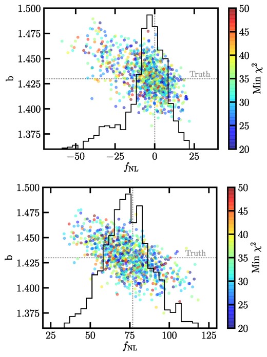
The best-fitting estimates of b and fNL from fitting 1000 lognormal mocks with fNL = 0 (top) and 76.9 (bottom) in the DESI footprint. No mitigation is applied to the mocks. The truth values are represented by vertical and horizontal lines.
For infinitesimal values of fNL, the derivative becomes asymptotically independent from fNL while for large values of fNL it decreases as 2/fNL. This implies that for the fNL = 0 mocks, the likelihood is more likely to be skewed toward negative values.
B2 Contaminated mocks
Our non-linear neural network-based approach is applied to the fNL = 0 and 76.9 mocks. We only consider the methods that include running the neural network with three, four, and nine imaging systematic maps. The measured mean power spectrum of the mocks are shown in Fig. B4 for fNL = 0 (left) and 76.9 (right). The solid and dashed curves show the measurements respectively from the clean and contaminated mocks.
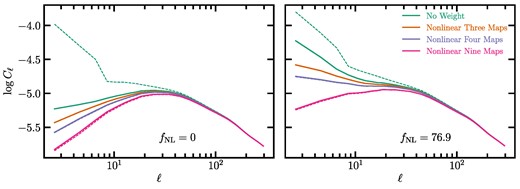
The mean power spectrum of the fNL = 0 and 76.9 mocks with (dashed) and without (solid) imaging systematics before (‘No Weight’) and after applying the non-linear cleaning method with three, four, and nine maps.
We find that the imaging treatment has removed some of the true clustering signal, and the amount of the oversubtraction is almost the same regardless of whether the mocks have systematics. The oversubtraction induces biases in the fNL constraints, as summarized in Table B2. The oversubtraction at low ℓ is so high that we get a poor fit after applying the mitigation with the non-linear three maps approach, for example, χ2 = 86.8 for the clean fNL = 0 mocks.
The best-fitting and marginalized estimates for fNL from fitting the mean power spectrum of the mocks before and after corrections using the non-linear approach with various combinations of the imaging systematic maps. The covariance is scaled to represent the error on the mean power spectrum. The estimates are not accounted for overcorrection, and therefore are subject to mitigation systematics.
| fNL + Mitigation systematics | ||||||
|---|---|---|---|---|---|---|
| Mock / fNL | Method | Best fit | Mean | |$68\,\mathrm{ per\,cent}$| CL | |$95\,\mathrm{ per\,cent}$| CL | χ2 (dof =34) |
| Clean 0 | No weight | 0.36 | 0.36 | 0.06 < fNL < 0.65 | −0.23 < fNL < 0.94 | 35.7 |
| Clean 0 | Three maps | −11.64 | −11.65 | −12.00 < fNL < −11.30 | −12.34 < fNL < −10.97 | 86.8 |
| Clean 0 | Four maps | −20.14 | −20.13 | −20.44 < fNL < −19.82 | −20.74 < fNL < −19.52 | 472.8 |
| Clean 0 | Nine maps | −26.91 | −26.92 | −27.16 < fNL < −26.68 | −27.39 < fNL < −26.46 | 5481.0 |
| Contaminated 0 | Three maps | −12.12 | −12.13 | −12.48 < fNL < −11.78 | −12.83 < fNL < −11.44 | 94.0 |
| Contaminated 0 | Four maps | −20.97 | −20.98 | −21.28 < fNL < −20.67 | −21.58 < fNL < −20.37 | 556.3 |
| Contaminated 0 | Nine maps | −28.13 | −28.13 | −28.36 < fNL < −27.90 | −28.59 < fNL < −27.67 | 6760.5 |
| Clean 76.9 | No weight | 77.67 | 77.67 | 77.17 < fNL < 78.16 | 76.71 < fNL < 78.64 | 38.8 |
| Clean 76.9 | Three maps | 54.57 | 54.57 | 54.14 < fNL < 55.01 | 53.72 < fNL < 55.45 | 603.5 |
| Clean 76.9 | Four maps | 38.38 | 38.38 | 37.99 < fNL < 38.78 | 37.60 < fNL < 39.16 | 537.0 |
| Clean 76.9 | Nine maps | 6.04 | 6.04 | 5.72 < fNL < 6.36 | 5.41 < fNL < 6.67 | 694.0 |
| Contaminated 76.9 | Three maps | 54.01 | 54.00 | 53.57 < fNL < 54.44 | 53.15 < fNL < 54.86 | 588.0 |
| Contaminated 76.9 | Four maps | 37.48 | 37.49 | 37.09 < fNL < 37.88 | 36.70 < fNL < 38.27 | 510.7 |
| Contaminated 76.9 | Nine maps | 4.59 | 4.58 | 4.26 < fNL < 4.90 | 3.95 < fNL < 5.22 | 649.7 |
Using the calibration parameters presented in Section 3.7, we account for the shift in the fNL constraints caused by the imaging systematic mitigation. We show the marginalized probability distributions on fNL before and after accounting for the overcorrection in the right and left panels of Fig. B5.
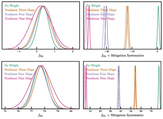
Probability distributions of fNL from the mean power spectrum of the fNL = 0 (top) and fNL = 76.9 (bottom) mocks before and after mitigation with the non-linear methods using three, four, and nine maps. The dashed (solid) curves show the distributions for the contaminated (clean) mocks. Left: the posteriors are adjusted to account for the overcorrection effect. Right: the posteriors are subject to the overcorrection effect, and thus the scaling of fNL values is biased due to mitigation.
