


ABSTRACT
Photometric completeness affects the photometry of stars in crowded regions such as the cores of star clusters. Some analysis such as deriving the structural parameters of star clusters using radial density profile is heavily affected by photometric completeness and the classical techniques to map this completeness in a given field are very expensive computationally. In most surveys, for example, the large quantity of data makes it impracticable to estimate the completeness using the traditional method for the whole sample due to time and computational requirements. In this work, we present a new method that is significantly faster and results in similar completeness curves and maps as the traditional approach, providing a great first-step completeness estimator for a large sample of data. Using the completeness corrected data for each cluster we built radial density profiles improving significantly the inner portion of the profile; we also fitted the King model to them, determining the clusters’ structural parameters based on a more realistic cluster profile. In this preliminary analysis, we derived structural parameters for nine selected clusters covering a range of core radii (5–40 arcesc) and tidal radii (40–180 arcesc) and discuss how the photometric completeness affects the determination of these parameters when we count stars to trace the radial profile of a star cluster.
1 INTRODUCTION
In any observation of point sources (stars), the detection of all stars along a given line of sight may be hampered if stars are superimposed on others. This effect is often referred to as confusion (see, for instance, Roseboom et al. 2010; Leschinski & Alves 2020; Kramer et al. 2022). Additionally, fainter objects tend not to be detected due to the presence of brighter nearby objects. This difficulty is accentuated by the sensitivity of the instrument, the brightness of the sky depending on the wavelength, and the spatial resolution that can be dominated by either the atmospheric seeing or the aperture of the telescope. These effects increase in denser fields like a stellar cluster. Given this unavoidable observational difficulty, it is necessary to investigate the percentage of stars that are effectively sampled, yielding an estimate of how incomplete a given stellar field is in terms of magnitude depth, and position. Bolte (1989) showed how the completeness factor was critical in the production of luminosity functions for M30.
Incomplete observations can lead to a non-uniform spatial distribution of the detected stars within a cluster. The resulting spatial distribution may not accurately represent the true distribution of stars which can affect measurements of cluster size, density, and other structural parameters as shown in Dias et al. (2014). For instance, stellar completeness can lead to an under representation of low-mass stars, resulting in a bias towards higher mass stars in the analysis and leading to an underestimation of the overall mass of the cluster and the degree of mass segregation present within it (Bolte1989).
Traditionally, the completeness analysis is made after an onerous computational process where artificial stars are added to the raw images iteratively at low densities and small range of magnitudes in order to avoid super populating the image with artificial stars and creating artificial confusion instead of testing it (e.g. Bolte 1989, 1994; Bergbusch 1996; Piotto et al. 1999; Da Rocha et al. 2002; Hargis, Sandquist & Bolte 2004; Fekadu, Sandquist & Bolte 2007; Maia, Moraux & Joncour 2016; Maia et al. 2019). This leads to the creation of dozens of different artificial images for a single star cluster. The completeness in each magnitude interval in terms of the number of recovered artificial stars is then derived after performing the photometry in each of the images (e.g. Santiago et al. 2001; Kerber et al. 2002; Dias et al. 2014).
Hu et al. (2010, 2011) proposed a method where artificial stars are randomly added to the star catalogue instead of the images. They applied this method to Hubble Space Telescope (HST) data and got similar results to the traditional approach, gaining significant computational time. They did not create any artificial images and then there was no need to perform photometry in each step. In another study, Li, de Grijs & Deng (2013) compared the analysis by Hu et al. (2010) with the traditional approach, concluding that while both methods perform well in low-density regions, the prior method fails to replicate accurate results in high-density regions. This discrepancy is attributed to the presence of bright (and their diffraction patterns) and saturated stars, highlighting the critical role of extended sources in such analysis.
In the line of Hu et al. (2010, 2011) procedure and considering the impact of extended sources according to Li et al. (2013), we implemented a method to evaluate the completeness of stars in ground-based observations data, in our case, taken from the SOuthern Astrophysical Research (SOAR) Telescope through the VIsible Soar photometry of star Clusters in tApii and Coxi HuguA (VISCACHA) survey (Maia et al. 2019) for nine clusters from both the Small Magellanic Cloud (SMC) and the Large Magellanic Cloud (LMC). Differently from HST data, the characteristics of our observations were heterogeneous, depending on different variables involved in the observations such as the variable seeing and airmass and the performance of the SOAR adaptive optics module imager (SAMI) (Tokovinin et al. 2016), unlike Hu et al. (2011) work, which used more homogeneous catalogues due to the absence of these effects in space observations.
The Magellanic Clouds (MCs) are an interesting pair of dwarf galaxies. Due to their proximity to the Milky Way (MW), with the LMC and SMC being roughly 50 and 60 kpc away from the Sun (Westerlund 1997; Pietrzyński et al. 2019; Graczyk et al. 2020), it is possible to resolve individual stellar populations within them. This fact makes them important targets to study the galactic evolution process on a general scale. Over the years, many observations have taken place not only in the MCs but also in the structures around the galaxies.
There are numerous evidences that the MCs are interacting with each other as well as with the MW. For instance, structures such as the Magellanic Bridge, and the Magellanic Stream, as well as the observed warp in the disc-like structure of the LMC (Weinberg 2000; Olsen & Salyk 2002; Choi et al. 2018; Saroon & Subramanian 2022) can be accounted for the gravitational interaction between the LMC and the SMC, including a close, and recent, encounter (Yoshizawa & Noguchi 2003; Besla et al. 2012). This is also supported by the relative orientation of their 3D velocities (Kallivayalil et al. 2013). The Leading Arm, which is the counterpart of the Magellanic Stream, was first confirmed by Putman et al. (1998), and its origins lie within tidal interactions. In fact, all these substructures are signatures of the interactions between the MCs and the MW (Nidever et al. 2010; Diaz & Bekki 2012; D’Onghia & Fox 2016).
In the context of the MCs, Bica & Schmitt (1995) and Bica et al. (2020) made a great effort to catalogue the system’s star clusters focusing on the SMC. It is known that tidal forces impact the dynamical evolution and dissolution (Bastian et al. 2008) of star clusters, which leaves marks in their stellar content that can be explored by analysing the cluster’s structure (Werchan & Zaritsky 2011; Miholics, Webb & Sills 2014) and mass distribution (Glatt et al. 2011). A good completeness estimation is essential for obtaining reliable structural parameters, that can be used to investigate this phenomenon in the MCs.
Observation of clusters with relatively low surface brightness requires the utilization of more sensible instruments equipped with AO which provide better resolution and photometric depth (Piatti & Bica 2012). In this sense, the VISCACHA Survey has been conducting observations with a well-defined observational strategy. Since 2015, the survey has observed a remarkable number of over 200 clusters across both the SMC and the LMC, as well as clusters situated in the Magellanic Bridge employing AO and thus enhancing the quality of the observations. They have yielded a wealth of valuable data that contribute to our understanding of these objects.
In this work, we present a new method to estimate the photometric completeness of stars in dense fields, using it to provide the structural parameters for nine MCs star clusters. In Section 2, we present an overview of the observations and data utilized. The methodology is described in Section 3, and in Section 4, we briefly explain our procedures to optimize it. In Section 5, we employ the methods to create radial density profiles (RDPs) of each region. The first results are shown in Section 6 and our concluding remarks and perspectives are presented in Section 7.
2 OBSERVATIONS AND DATA
For the current study, we have used the same data as presented in Maia et al. (2019), which consists of a sample of nine clusters, four from the SMC and five from the LMC. These clusters were selected because they illustrate different concentrations, total brightness, and physical parameters. The primary objective of this work is to introduce a new method for estimating completeness for ground-based observations, designed to be applicable to large data sets with lower time investment. In the interest of consistency and to enable a direct comparison with their results, we have employed the identical star catalogue for each cluster. Furthermore, we have utilized the predetermined cluster centres, also established in Maia et al. (2019), for our RDP analysis.
By using the same data set, catalogue, and cluster centres, we establish a solid foundation for our methodology and facilitate a comprehensive comparison with the previous results. This approach enables us to accurately assess the advancements made in estimating completeness and further our understanding of the observed clusters in the context of the VISCACHA Survey.
Table 1 provides a comprehensive overview of the observations conducted for the clusters analysed in this study. The table presents the precise positions of each cluster in right ascension (RA) and declination (Dec.), along with the dates when the observations took place and the specific filters employed.
Log of observations for the clusters analysed in this paper.
| Name | RA [h:m:s] | Dec [|$^{\circ }$|:′:″] | Date of observation [DD/MM/YYYY] | Filters | Seeing [arcsec] | IQ [arcsec] | AO? |
|---|---|---|---|---|---|---|---|
| SMC | |||||||
| AM3 | 23:48:59 | |$-$|72:56:43 | 04/11/2016 | V, I | 1.2, 1.1 | 0.5, 0.4 | ON |
| HW20 | 00:44:47 | |$-$|74:21:46 | 27/09/2016 | V, I | 1.2, 0.9 | 0.6, 0.5 | ON |
| K37 | 00:57:47 | |$-$|74:19:36 | 04/11/2016 | V, I | 0.8, 0.8 | 0.5, 0.4 | ON |
| NGC796 | 01:56:44 | |$-$|74:13:10 | 04/11/2016 | V, I | 1.0, 0.9 | 0.6, 0.5 | ON |
| LMC | |||||||
| KMHK228 | 04:53:03 | |$-$|74:00:14 | 11/01/2016 | V, I | 1.1, 1.0 | 1.1, 1.0 | ON |
| OHSC3 | 04:56:36 | |$-$|75:14:29 | 02/12/2016 | V, I | 1.0, 1.0 | 1.0, 1.0 | OFF |
| SL576 | 05:33:13 | |$-$|74:22:08 | 29/11/2016 | V, I | 1.3, 1.0 | 1.2, 1.0 | ON |
| SL61 | 04:50:45 | |$-$|75:31:59 | 09/01/2016 | V, I | 0.9, 0.8 | 0.7, 0.6 | ON |
| SL897 | 06:33:01 | |$-$|71:07:40 | 23/02/2016 | V, I | 1.5, 1.4 | 1.1, 0.9 | ON |
Notably, despite the fact that all clusters were observed under similar seeing, there are discrepancies in the delivered image quality (IQ), which represents the measure of seeing after the application of AO correction. This discrepancy can be attributed to the inherent variability of free-atmosphere seeing, which remains uncorrected by the ground-layer adaptive optics (GLAO) employed in the observations.
The catalogue lists the positions of stars in RA and Dec. and also in coordinates X and Y in pixels of the detector, in binned mode (2 × 2). The catalogue also lists the result of the photometric calibration presenting the magnitudes in V and I of each observed star. In our work, we used only stars present in both V and I catalogues.
Starting with AM3 and K37 clusters as prototypes for our study, we initially performed a complete analysis of these clusters and then expanded to the other seven clusters in our sample. We choose these objects because they represent two completely different types of clusters. While AM3 has a relatively small number of stars and lies in a low-density field, K37 is more populous and fills the image making it harder to discern the cluster from the background. After performing the analysis for these clusters, the remaining seven clusters were classified as AM3-like or K37-like, according to the similarity of their images to one or the other of these clusters.
3 METHODOLOGY
3.1 Artificial stars grid
The first step in our analysis is to create an artificial stars grid, with a constant magnitude, equally spaced through the plane defined by coordinates X and Y. We then compare the position and magnitude of the observed stars with each artificial star to determine if it is recovered or not (see Section 3.2).
Grids with different magnitudes (in V and I bands) are simulated, covering the whole range of magnitudes of the original catalogue. The separation (D) between each artificial star in the grid is a free parameter, proportional to the IQ of the images (see Section 3.2). In this way, D allows us to quantify what is the influence of the grid density on the subsequent analysis.
Fig. 1 shows an example of the artificial stars grid overlapped to the K37 stars coordinates, with size indicating their V magnitude. It is possible to visualize the distribution of observed stars in the images and their positioning in the grid. We can observe the regions with greater star density where we expect the centre of the cluster to be located, as well as regions with low density which are also important for checking completeness behaviour free of crowding effects, especially for fainter magnitudes.
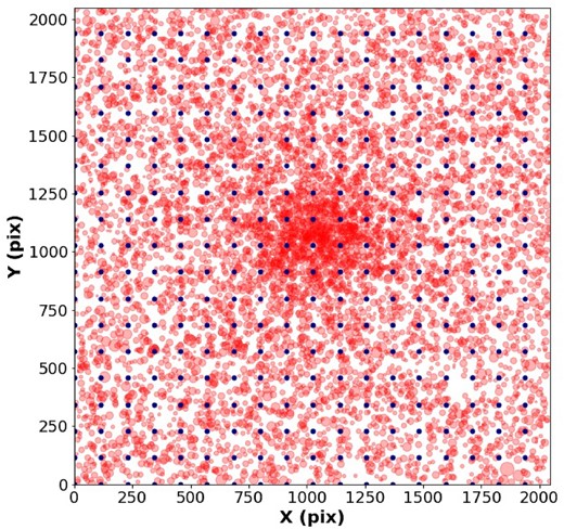
Illustration of the artificial stars grid overlapped with observed stars of K37. Dots represent artificial stars and circles, the observed stars dimensioned by their magnitude, with brighter stars being represented by bigger circles.
3.2 Merged stars analysis
Determining which and how many artificial stars are merged with observed ones is the first step in deriving the completeness. Initially, we compare the distance, in pixels, between each observed and artificial stars in the grid. Hu et al. (2011) showed that, for HST observations, a distance (|$d_{\mathrm{ lim}}$|) of 2 pixels is a good approximation to determine that the artificial star is merged with the observed one. This value is not necessarily applicable for ground-based observation though, as the turbulence effects of the atmosphere must be taken into account. It can be accounted in the form of the variable seeing in each observation, which measures the full width at half-maximum (FWHM) of the stars in an image.
In practice, the natural seeing is improved by the instrument correction provided by the SOAR Telescope Adaptive Module (SAM) (Tokovinin et al. 2016) used in the observations to determine the IQ of each image. SAM is a GLAO module that utilizes a Rayleigh laser guide star positioned approximately 7 km from the telescope. It works by partially compensating the turbulence near the ground. We then presume that the best value of separation that defines the merging of artificial and observed stars is a function of each observation IQ.
We determined the occurrence of positional merging by calculating the Euclidean distance between each artificial star and its corresponding observed star from the original catalogue. We analysed each artificial star individually to avoid interference from other artificial stars in the grid. Our approach ensures that two artificial stars were never merged with each other. This methodology allowed us to freely adjust the grid density for our analysis, providing flexibility in evaluating the effects of different density levels on positional merging. This flexibility is not possible when performing the traditional method due to confusion.
As previously cited, Table 1 shows the atmospheric seeing and IQ of each observation, defined in arcseconds. Following the reasoning of the Rayleigh criterion, we define the limiting separation for resolving sources |$d_{\mathrm{ lim}}$| as a constant times the image IQ. Since we are working on a pixel scale, we divided the IQ values by 0.09, which is the scale of arcseconds per pixel of the binned CCD. The |$d_{\mathrm{ lim}}$| value is then defined by
To initiate our analysis, we adopted a starting point value of a = 2 for the constant in the calculation of the limiting separation |$d_{\mathrm{ lim}}$|, taking inspiration from the methodology employed by Hu et al. (2011) as a starting point. This initial value provides a baseline reference for our sample.
However, we subsequently fine-tuned the value of a to align more precisely with the properties and requirements of our data. We did this by performing a series of tests, comparing with the literature date and then performing sanity checks to find the best values. More details will follow on Section 4. This iterative process of fine-tuning the value of a allows us to account for any distinctive factors within our data and ensures that our calculations are aligned with the specific goals and requirements of our study.
Using the sklearn (Pedregosa et al. 2011) package in python we employed a nearest neighbour algorithm with the Euclidean metric to identify and calculate the distance between each artificial star and the closest observed star. We set as positionally merged every artificial star with distance lower than |$d_{\mathrm{ lim}}$| from the closest observed star. As an initial approach, this procedure ensures that despite treating stars as point-like sources, we reduce potential limitations addressing the merging of artificial stars even if they are not too close to the centre of the observed stars.
After identifying positionally merged stars, the subsequent step involved obtaining the magnitude difference between them (Hu et al. 2011). For each pair of merged stars, we compared the magnitudes of the artificial star and the observed star.
To determine the completeness of artificial stars, we employed a Monte Carlo simulation where the magnitude of each observed star varies with a normal distribution to reflect its uncertainty. Utilizing 100 artificial stars in each position we considered as undetected the artificial stars with magnitude exceeding the sampled magnitudes of the observed stars. Conversely, if the magnitude of the artificial star was lower than sampled magnitude of the observed star, we determined that the artificial star was successfully recovered. The completeness of the artificial star at a given position was then quantified as the fraction of stars recovered in the Monte Carlo simulation.
Finally, as demonstrated by Li et al. (2013), the existence of extended sources on imaging fields causes stellar completeness depletion, which is not considered whenever this kind of analysis is done based on stellar proximity and flux using the catalogues rather than based on the classical artificial star tests (ASTs) over the images. These extended sources include saturated stars and their bleeding pixels, bright stars (plus diffraction pattern) and galaxies enhancing the background level around their centres, cosmic rays, and bad pixels remaining from the reduction process.
Li et al. (2013, see their appendix A) employed sources flagged as extended during the reduction process of HST images of dense clusters to estimate their effect on the stellar completeness. They compared AST-based completeness with catalogue-based completeness and concluded that a much better agreement is reached after the correction of the latter for extended sources was applied, that is, stars are not recovered once they blend with extended sources. The effect of extended sources is more significant for populous, dense clusters with young stellar populations due to their bright main sequence, but may also be important for older populations with bright giants (e.g. SL 576). However, most of the full VISCACHA sample contains low-surface brightness clusters, immersed in the low-density stellar fields of the MCs’ outskirts (Santos João et al. 2020), therefore we expect a mild impact on the completeness curves of most of the clusters.
On the other hand, since this technique may be applied to images/catalogues employing different instrumental setup and observations, and acknowledging the importance of extended objects on the catalogue-based completeness analysis, we pursued a similar approach as Li et al. (2013).
One of the subproducts of the reduction process is the residual image (original image minus the point spread function-fitted synthetic image), which contains all extended sources not resolved by the stellar photometry software (Diolaiti et al. 2000); see Maia et al. (2019) for details. We analysed the residual image, computing the median, and standard deviation of the count numbers across the entire image. Then we mark all pixels with negative counts as saturated. Subsequently, we established a threshold where the count number exceeded the median plus 3–5 times the standard deviation to enhance extended objects. Pixels with fewer counts than this threshold were assigned a value of 0 (zero), indicating no extended sources, while pixels with more counts were assigned a value of 1 (one), representing the presence of extended sources. We then cross-matched the artificial stars grid with the generated mask, setting the final completeness to 0 in regions marked with extended sources.
To provide a visual representation of the algorithm’s flow, we created Fig. 2, a flowchart illustrating the steps followed by our algorithm to determine if the artificial stars were recovered or not. This flowchart offers a clear overview of the decision-making in this process. By implementing this methodology, we successfully evaluated the recovery of artificial stars based on both magnitude differences and positional merging with observed stars.

Sequence followed by the algorithm to determine if artificial stars are recovered or not.
Following the application of this methodology to grids with varying magnitudes, we observed that the completeness of artificial stars differed accordingly. It is expected that the completeness of an artificial star in a specific position diminishes as the magnitude increases.
3.3 Completeness maps
After calculating the completeness of artificial stars, we built maps that defined the completeness over the coordinates (in pixels) of the grid. In this analysis, we created an algorithm that scans the 2D space through a square box with sides proportional to the separation between artificial stars. The number of artificial stars inside the box (from now on named as Nbox) is fixed and the completeness of the central coordinates of the box is given by the mean completeness of the artificial stars inside it.
For a given magnitude of the grid, we calculate the mean completeness of the central point of the box and then we moved it in one of the axes recalculating this fraction until the whole axis is covered. Then we moved the box through the other axis, repeating the process until the whole grid is swept. As the box approached the borders of the grid, its size was appropriately adjusted to ensure that it remained within the grid boundaries. Consequently, Nbox decreased near the borders of the grid due to the reduced box size, accounting for the border effects accurately. Fig. 3 provides a visual illustration of this procedure, highlighting how the box is moved and adjusted to cover the entire grid.
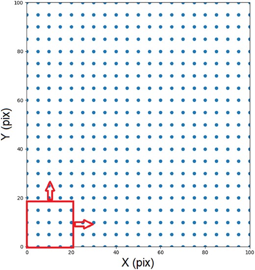
Illustration of the square box created by the algorithm to build the completeness maps.
Fig. 4 displays the completeness maps for four different magnitude grids of artificial stars. In these maps, brighter colours indicate higher completeness, while darker colours represent lower completeness. They provide a visual representation of the variation in recovery rates across different regions of the observed field. The decreasing completeness towards the cluster centre is expected as these regions are denser than the outskirts, resulting in a lower recovery rate for artificial stars. This trend also becomes more apparent as the magnitudes of the artificial stars decrease, indicating that fainter sources are more challenging to recover in the central regions.
3.4 Completeness of observed stars
Using the values obtained for the completeness in each point of the grid for each magnitude we were able to define the completeness for each observed star. Taking the coordinates and magnitudes of these stars, we used a nearest neighbours algorithm to compare each of them with our completeness map in every magnitude and select, among the two closest magnitude maps (i.e. one brighter and one fainter than the observed star), the four closest points for which completeness were calculated in those maps. Completeness for the observed star was then calculated by performing a linear interpolation with the completeness values in both maps.
In Fig. 5, we show the completeness of the observed stars and their position for the case of K37, in equatorial coordinates. There is a clear difference in completeness for stars in the regions closer to the centre of the clusters than in the outer regions. Fig. 6 depicts histograms illustrating the completeness corrected number of stars as a function of magnitude. In these completeness corrected histograms, each star contributes as ‘counts’ in the corresponding magnitude bin, weighted by the inverse of its completeness value. Notably, the histograms clearly demonstrate that the completeness correction has a more evident effect on fainter stars.
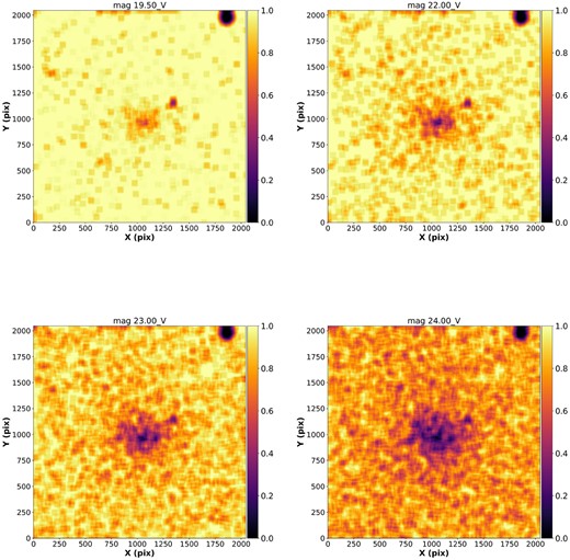
Photometric completeness in the V band for the K37 in different magnitudes using D = 1, |$d_{\mathrm{ lim}}$| = 1.5, and Nbox = 100. The colour bars shows the density of recovered artificial stars in the field, bright colours mean more recovered stars, and darker colours are less recovered stars.
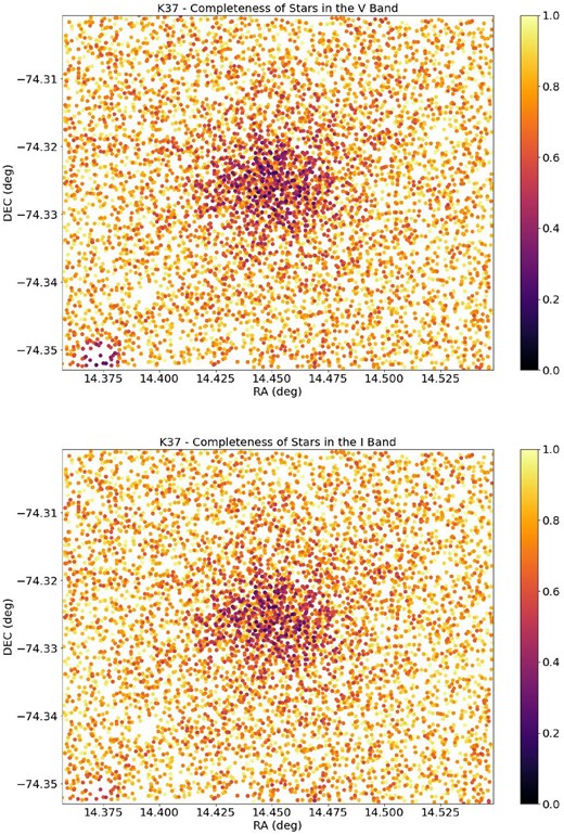
V and I photometric completeness of the observed stars of K37. Colour bar represents the completeness percentage, and darker points are more incomplete stars.
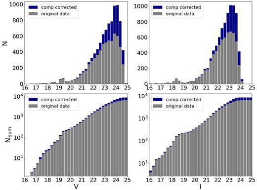
Histograms of completeness corrected number of stars per magnitude bins for the entire field of K37 in both V and I bands. Top panels are the non-cumulative histograms and bottom panels are the cumulative histograms.
The completeness maps in Fig. 5 reveal spatial variations in completeness, while the completeness corrected histograms in Fig. 6 show the impact of completeness on the distribution of stars across different magnitude bins. This shows the importance of accounting for completeness in order to accurately understand the observed stellar populations within the clusters.
3.5 Magnitude limit
In our study, we aimed to improve the reliability of our analysis by utilizing a series of histograms representing the number of stars within different magnitude bins, effectively depicting the luminosity function of the observed star clusters. We observed that, generally, the number of stars tends to increase with magnitude. Therefore, we set out to identify the peak value within each histogram, representing the most common magnitude range for stars within the clusters.
To establish a magnitude limit that encompasses the overall behaviour of the clusters, we adopted the mean value of the identified peaks across the different magnitude bins. By taking the average of these peaks, we account for variations in the luminosity function within each bin, creating a more representative and inclusive limit.
This approach, depicted in Fig. 7 for K37, allows us to include the majority of stars within the cluster while minimizing the potential inclusion of spurious or less reliable data points that may be associated with observational artefacts or biases. By focusing on the mean value of the peaks, we ensure a more precise characterization of this limit in the examined star clusters.
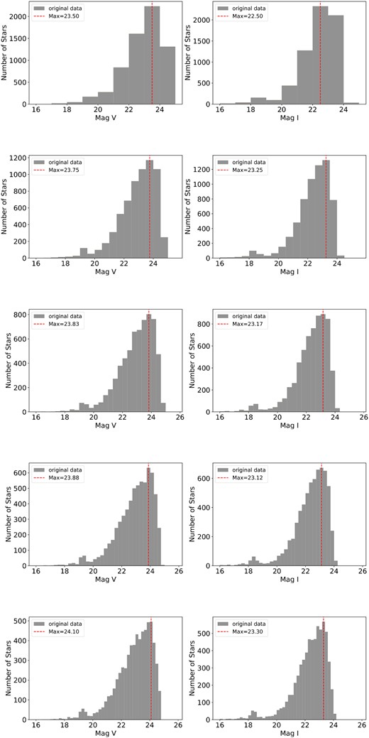
Procedure to determine the magnitude limit for the K37 cluster. The magnitude range is divided into bins of 1, 1/2, 1/3, 1/4, and 1/5 magnitudes. The histograms depict the occurrences of stars within the cluster at different magnitudes. The peak of occurrences in each histogram is identified and are represented by the dashed line in the centre of the highest bin, representing the magnitude limit within that bin. The mean value of these peak estimates is calculated to determine the definitive magnitude limit for the observed region.
Table 2 presents the magnitude limits determined in each of the clusters analysed (|$V_{\mathrm{ lim}}$|, |$I_{\mathrm{ lim}}$|). It is perceptible that although the IQ is generally lower in the I band, the magnitude limit in this band is brighter than in the V band.
V and I limiting magnitudes with corresponding masses and the magnitudes of the brightest clusters’ members according to Maia et al. (2019).
| Name | |$V_{\mathrm{ lim}}$| | m (M|$_\odot$|) | |$I_{\mathrm{ lim}}$| | m (M|$_\odot$|) | |$V_{\mathrm{ min}}$| | |$I_{\mathrm{ min}}$| |
|---|---|---|---|---|---|---|
| AM3 | 23.77 | 0.85 | 22.36 | 0.93 | 19.0 | 17.9 |
| K37 | 23.81 | 0.93 | 23.07 | 0.94 | 16.9 | 15.6 |
| NGC796 | 22.88 | 1.18 | 21.77 | 1.37 | 14.0 | 14.0 |
| HW20 | 23.35 | 1.06 | 22.57 | 1.10 | 16.7 | 15.2 |
| KMHK228 | 22.03 | 1.39 | 21.42 | 1.45 | 18.2 | 17.3 |
| OHSC3 | 22.22 | 1.12 | 21.77 | 1.11 | 18.2 | 17.3 |
| SL576 | 22.42 | 1.16 | 21.53 | 1.26 | 17.5 | 16.6 |
| SL61 | 22.77 | 1.09 | 22.02 | 1.11 | 17.0 | 15.3 |
| SL897 | 22.51 | 1.13 | 21.77 | 1.16 | 18.0 | 17.0 |
It is very important to mention that the considerable distance of the MCs implies that a significant fraction of stars will remain completely unseen regardless of the precision of the completeness estimations. Therefore, our analysis consider only stars above a certain mass threshold. This threshold was determined by interpolating the isochrones fitted by Maia et al. (2019) to the clusters Colour-Magnitude Diagrams (CMDs) and extracting the mass corresponding to our previously obtained magnitude limit. The mass limit is also presented in Table 2.
A limitation of our approach concerns the completeness of very bright stars, with discrepancies above 10 per cent in some cases. However, we evaluated the completeness for all stars catalogued, which encompassed stars as bright as 1–2 mag below the magnitude of the brightest cluster member stars (Maia et al. 2019; Dias et al. 2022). Although the lower magnitude completeness estimates are less accurate, we can always truncate our sample up to the limit of the clusters’ brightest members. From there to fainter stars the completeness is sufficiently reliable. The approximate magnitude of the brightest star (|$V_{\mathrm{ min}}$|, |$I_{\mathrm{ min}}$|) in each cluster is also presented in Table 2.
4 DETERMINATION OF FREE PARAMETERS
In order to determine the best values for the free parameters of our completeness analysis, that is, separation between each artificial star in the grid (D), distance limit to define if stars are merged (|$d_{\mathrm{ lim}}$|), and number of stars inside the box (Nbox) for building the completeness maps, we performed a series of trials for the clusters AM3 and K37. For each grid with different densities, we evaluated the completeness of the stars with different values of |$d_{\mathrm{ lim}}$| and Nbox. We also fitted RDPs as a way to optimize the proposed method.
We established that all clusters except for NGC796 and KMHK228 are K37-like in the division we made previously. Since IQ is an underlying quantity interfering with the optimum values of the free parameters, we propose that by tweaking these free parameters we can cover most of the reasonable weather conditions under which the star clusters were observed. In a more general case, if several telescopes and instruments are employed, additional factors should be taken into account.
To optimize the free parameters, we employed our methodology in the completeness estimation to the two prototype clusters using different values of free parameters: D = 1, 3, and 5 |$\times$| IQ, |$d_{\mathrm{ lim}}$| = 1, 1.5, 2, 3, 4, and 5 |$\times$| IQ, and Nbox = 16, 25, 49, and 100 stars as it will be described below.
4.1 Completeness comparison
For each of the combinations of D, |$d_{\mathrm{ lim}}$|, and Nbox, we evaluated the stellar completeness for AM3 and K37 and we compared with those derived by Maia et al. (2019). We then calculated the mean value of the difference (residual) between the completeness derived in our work and those from Maia et al. (2019).
To determine an equivalence index (|$\xi$|) between the methods, we took the mean square difference of the average values of the completeness in both methods for each bin of magnitude and calculated the average over the entire sample up to the magnitude limit established for the cluster. Therefore, the combinations of free parameters that are most equivalent to the method used by Maia et al. (2019) are those where the |$\xi$| are the lowest. The |$\xi$| values for K37 in both bands are shown in Table 3.
Equivalence indices |$\xi$| for K37 in both bands.
| |$\xi$|V | |$\xi$|I | |||||||
|---|---|---|---|---|---|---|---|---|
| D1 | ||||||||
| dlim | Box | Box | ||||||
| 16 | 25 | 49 | 100 | 16 | 25 | 49 | 100 | |
| 1.0 | 0.047 | 0.044 | 0.042 | 0.041 | 0.029 | 0.026 | 0.024 | 0.024 |
| 1.5 | 0.039 | 0.033 | 0.027 | 0.025 | 0.034 | 0.028 | 0.022 | 0.020 |
| 2.0 | 0.048 | 0.039 | 0.030 | 0.026 | 0.054 | 0.048 | 0.043 | 0.040 |
| 3.0 | 0.064 | 0.063 | 0.060 | 0.059 | 0.070 | 0.075 | 0.084 | 0.089 |
| 4.0 | 0.065 | 0.066 | 0.076 | 0.085 | 0.071 | 0.077 | 0.095 | 0.109 |
| 5.0 | 0.065 | 0.066 | 0.077 | 0.093 | 0.071 | 0.077 | 0.095 | 0.113 |
| D3 | ||||||||
| dlim | Box | Box | ||||||
| 16 | 25 | 49 | 100 | 16 | 25 | 49 | 100 | |
| 1.0 | 0.044 | 0.043 | 0.043 | 0.044 | 0.027 | 0.026 | 0.025 | 0.025 |
| 1.5 | 0.027 | 0.026 | 0.026 | 0.026 | 0.024 | 0.021 | 0.020 | 0.019 |
| 2.0 | 0.027 | 0.026 | 0.025 | 0.024 | 0.042 | 0.039 | 0.037 | 0.036 |
| 3.0 | 0.062 | 0.060 | 0.059 | 0.058 | 0.093 | 0.092 | 0.091 | 0.091 |
| 4.0 | 0.090 | 0.091 | 0.092 | 0.092 | 0.115 | 0.116 | 0.118 | 0.119 |
| 5.0 | 0.101 | 0.104 | 0.107 | 0.108 | 0.120 | 0.122 | 0.124 | 0.126 |
| D5 | ||||||||
| dlim | box | box | ||||||
| 16 | 25 | 49 | 100 | 16 | 25 | 49 | 100 | |
| 1.0 | 0.047 | 0.046 | 0.045 | 0.045 | 0.029 | 0.027 | 0.025 | 0.024 |
| 1.5 | 0.030 | 0.028 | 0.027 | 0.026 | 0.026 | 0.023 | 0.021 | 0.020 |
| 2.0 | 0.028 | 0.026 | 0.025 | 0.024 | 0.044 | 0.041 | 0.039 | 0.037 |
| 3.0 | 0.060 | 0.058 | 0.057 | 0.056 | 0.095 | 0.093 | 0.092 | 0.091 |
| 4.0 | 0.093 | 0.092 | 0.092 | 0.092 | 0.122 | 0.121 | 0.120 | 0.120 |
| 5.0 | 0.108 | 0.108 | 0.108 | 0.108 | 0.130 | 0.129 | 0.129 | 0.128 |
Figs 8 and 9 present the completeness curves of observed stars for both our method and the traditional approach and the residuals of this analysis in V and I bands, respectively. The limiting magnitudes and the magnitude of the brightest cluster member for each band are represented by the blue dashed line in both figures. The positive or negative values in the residuals indicate overestimation or underestimation of completeness by our method compared to traditional method. The figures showing the direct comparison between both methods for the remaining clusters are displayed in Appendix B.
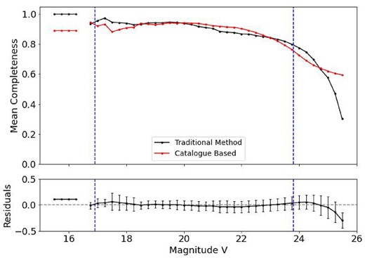
Top panel: completeness curves for K37 from both methods. The solid lines represent the mean completeness per magnitude bin obtained by the traditional method (Maia et al. 2019) and the values obtained by our proposed method. The dashed vertical lines represent |$V_{\mathrm{ min}}$| and |$V_{\mathrm{ lim}}$| values according to Table 3. Bottom panel: calculated residuals for the V band. The error bars are the standard deviation and the dashed horizontal line is positioned in 0 (zero). In both panels, the dots represent the magnitude bins where the mean completeness was calculated.
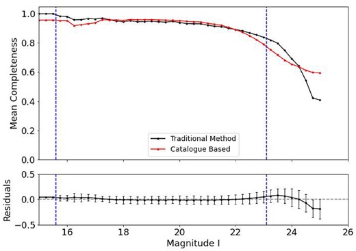
Completeness curves for K37 from both methods and the residuals for the I band. Details as in Fig. 8.
After conducting this analysis, we determined the optimal free parameters |$d_{\mathrm{ lim}}$| and Nbox according to the separation D for each cluster in each band. The overall completeness will then be calculated as the mean completeness of the three best combination of parameters. This smooths the estimations, as varying the grid density (D) allows us to access a different number of artificial stars in various positions, recovering different stars in each iteration. We then proceeded with our analysis of the RDP using the determined mean completeness. The best combination of free parameters for K37 are boldfaced in Table 3 and combinations of free parameters for the AM3 are presented in the Appendix A, as well as the best combinations in boldface.
5 RADIAL DENSITY PROFILE
5.1 Centre coordinates and frame borders
To construct a reliable RDP for the cluster, it is crucial to accurately determine the central coordinates. In this study, we utilized the central coordinates provided in Maia et al. (2019), which were determined iteratively by calculating the centroid of star coordinates within a visual radius. The iterative process allowed for precise adjustments at each step, resulting in more accurate central coordinate estimates.
The RDP of each cluster will be evaluated by considering the number of stars that fall within a sequence of annular regions of different radii, constructed around the cluster centre. Due to the instrument’s finite field of view, if we evaluate the RDP for increasingly larger distances, the external annular bins will eventually extend beyond the image boundaries. To properly determine the stellar density in those regions, we analytically calculate the amount of the total area of each annulus that falls within the image.
Although this approach allows us to evaluate the RDPs for radii larger than the distance of the cluster centre to the closest image border, the area corrections cannot be performed indefinitely, since the annular bins would, at some point, be completely out of the image. Even before that, the proportion of the area of the external bins that fall within the image, compared to their total area is too small for a reliable estimation of the stellar density. Therefore, when evaluating the RDPs, we truncate the maximum distance from the cluster centre up until the area of the largest annular bins that fall outside the image is approximately 80 per cent of its total area.
By considering the central coordinates determined iteratively and doing appropriate correction to the area, we ensured that the RDP extended far enough to the cluster centre to provide an accurate estimate of the tidal radius.
5.2 Construction of the RDP
To construct the RDPs, we first consider the original stellar counts in each annular bin, without assuming completeness of stars. The density of stars in each annular bin, as a function of radius, is calculated using the formula:
Here, |$\rho$| represents the density of stars, |$N_{\text{Stars}}$| denotes the number of stars within the annular bin, and |$A_{\text{Ring}}$| corresponds to the area of the annular bin. It is important to note that the first annular bin is treated as a circle, not a ring.
Subsequently, we constructed the completeness-corrected profiles, taking into account the completeness associated with each individual observed star. The correction factor for each observed star is given by the inverse of its completeness value. The corrected number of stars per bin is then obtained by summing up the individual corrected values, as expressed in equation (3):
where the index i represents the observed star, and |$\text{cmp}_i$| denotes the completeness of that particular star. Consequently, the corrected density is calculated as:
To ensure that the completeness is not overcorrected, we set a lower limit for the individual completeness value equal to 0.5. Consequently, if a star has a completeness value lower than 0.5, its maximum contribution to the corrected count (equation 3) is 2. This adjustment prevents an excessive correction of the completeness value and maintains the accuracy of the analysis.
5.3 Model fit to the RDP
Once the RDPs are built, the cluster structural parameters are determined by fitting an analytical model to them. Many models have been developed and used over the years to characterize Galactic clusters (e.g Plummer 1911; King 1962; Wilson 1975; Elson, Fall & Freeman 1987). In our study, we applied the empirical King (1962) model to the completeness corrected RDPs of each cluster (Dias et al. 2016; Maia et al. 2016, 2019). We selected this model because, in addition to being widely used in the characterization of Galactic star clusters, it was also used in the paper we are using as comparison. The model is described by the equation:
In this equation, |$\rho _{0}$| represents the central stellar density, |$r_{c}$| denotes the core radius, |$r_{t}$| corresponds to the tidal radius, and |$\rho _{s}$| represents the stellar field density. It is assumed that |$r_{t}$| is significantly larger than |$r_{c}$|.
To estimate the stellar field density, we counted the number of stars in areas located at the outskirts of the observed region, which are considered representative of the background stellar density.
To fit the non-linear function of equation (5) to our data, we utilized a least-squares algorithm. By applying this fitting process, we obtained estimates for |$\rho _{0}$|, |$r_{c}$|, |$r_{t}$|, and |$\rho _{s}$|. Fig. 10 shows the fit to the completeness-corrected RDP of K37 in the V and I bands, as well as the RDP before the completeness correction analysis.
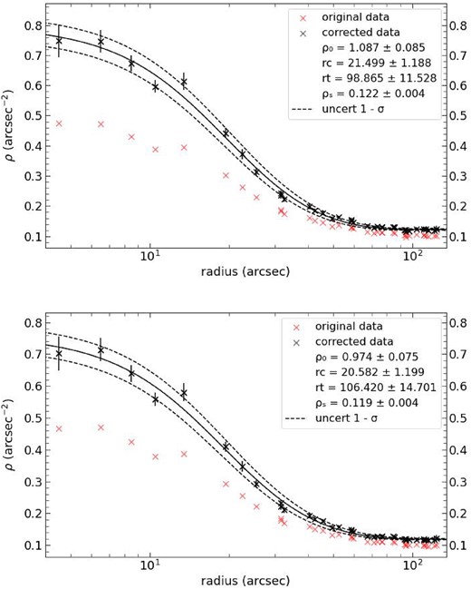
Fit to the completeness corrected RDP of K37, denoted by the black ‘x’ points. The RDP points before the completeness correction analysis are also shown denoted by the red ‘x’ points. The top panel shows the fit for the V band and the bottom panel shows the fit for the I band.
6 FIRST RESULTS
Table 4 presents a summary of the structural parameters obtained from completeness-corrected data for our cluster sample. These parameters were previously determined using various techniques, as documented in prior studies (see e.g. Kontizas & Kontizas 1985; Bica & Schmitt 1995; Hill & Zaritsky 2006; Piatti & Bastian 2016; Maia et al. 2019; Santos et al. 2020). In this section, we will briefly discuss our findings in comparison to those reported in the literature, with a particular focus on the results presented by Maia et al. (2019) and Santos et al. (2020), both of which are also included in Table 4 for reference.
Structural parameters resulted from the King fit to RDP for the sample analysed in the V and I bands.
| Cluster | |$\rho _0$| | |$\rho _s$| | |$r_c$| | |$r_t$| |
|---|---|---|---|---|
| (stars arcmin−2) | (stars arcmin−2) | (arcmin) | (arcmin) | |
| AM3 (V) | 0.493 |$\pm$| 0.008 | 0.004 |$\pm$| 0.001 | 6.7 |$\pm$| 0.2 | 74.5 |$\pm$| 6.6 |
| (I) | 0.412 |$\pm$| 0.013 | 0.004 |$\pm$| 0.001 | 4.7 |$\pm$| 0.2 | 65.2 |$\pm$| 7.7 |
| (Maia) | 0.09 |$\pm$| 0.02 | 0.0010 |$\pm$| 0.0001 | 5.6 |$\pm$| 0.8 | 54 |$\pm$| 8 |
| (Santos) | – | – | 4.6 |$\pm$| 1.6 | 54 |$\pm$| 44 |
| K37 (V) | 1.087 |$\pm$| 0.085 | 0.122 |$\pm$| 0.004 | 24.5 |$\pm$| 1.2 | 98.8 |$\pm$| 11.5 |
| (I) | 0.974 |$\pm$| 0.075 | 0.119 |$\pm$| 0.004 | 20.6 |$\pm$| 1.2 | 106.4 |$\pm$| 14.7 |
| (Maia) | 0.47 |$\pm$| 0.06 | 0.0236 |$\pm$| 0.0067 | 11.3 |$\pm$| 1.5 | 83 |$\pm$| 17 |
| (Santos)|$\dagger$| | 0.54 |$\pm$| 0.04 | 0.102 |$\pm$| 0.003 | 22 |$\pm$| 3 | 117 |$\pm$| 18 |
| NGC796 (V) | 0.918 |$\pm$| 0.018 | 0.005 |$\pm$| 0.002 | 8.2 |$\pm$| 0.3 | 65.5 |$\pm$| 5.4 |
| (I) | 0.728 |$\pm$| 0.015 | 0.004 |$\pm$| 0.002 | 8.4 |$\pm$| 0.3 | 68.4 |$\pm$| 6.1 |
| (Maia) | 0.7 |$\pm$| 0.3 | 0.0015 |$\pm$| 0.0005 | 3.2 |$\pm$| 0.5 | 97 |$\pm$| 9 |
| (Santos) | – | – | 2.8 |$\pm$| 0.5 | 128 |$\pm$| 18 |
| HW20 (V) | 0.349 |$\pm$| 0.077 | 0.098 |$\pm$| 0.011 | 12.9 |$\pm$| 2.1 | 58.4 |$\pm$| 19.0 |
| (I) | 0.322 |$\pm$| 0.072 | 0.081 |$\pm$| 0.009 | 12.0 |$\pm$| 2.1 | 55.5 |$\pm$| 19.0 |
| (Maia) | 0.13 |$\pm$| 0.06 | 0.0307 |$\pm$| 0.0095 | 10.8 |$\pm$| 2.0 | 37 |$\pm$| 11 |
| (Santos)|$\dagger$| | 0.54 |$\pm$| 0.04 | 0.102 |$\pm$| 0.003 | 18 |$\pm$| 4 | 56 |$\pm$| 7 |
| KMHK228 (V) | 0.102 |$\pm$| 0.047 | 0.014 |$\pm$| 0.002 | 21.4 |$\pm$| 5.2 | 51.2 |$\pm$| 11.9 |
| (I) | 0.110 |$\pm$| 0.030 | 0.017 |$\pm$| 0.002 | 19.5 |$\pm$| 3.2 | 58.6 |$\pm$| 12.1 |
| (Maia) | 0.11 |$\pm$| 0.05 | 0.0256 |$\pm$| 0.0029 | 19.8 |$\pm$| 5.9 | 68 |$\pm$| 16 |
| (Santos)|$\dagger$| | 0.06 |$\pm$| 0.01 | 0.015 |$\pm$| 0.001 | 15 |$\pm$| 5 | 66 |$\pm$| 21 |
| OHSC3 (V) | 0.335 |$\pm$| 0.015 | 0.017 |$\pm$| 0.002 | 6.6 |$\pm$| 0.4 | 70.8 |$\pm$| 16.3 |
| (I) | 0.331 |$\pm$| 0.015 | 0.018 |$\pm$| 0.003 | 6.7 |$\pm$| 0.5 | 77.9 |$\pm$| 20.6 |
| (Maia) | 0.6 |$\pm$| 0.1 | 0.0129 |$\pm$| 0.0037 | 4.3 |$\pm$| 0.7 | 42 |$\pm$| 6 |
| (Santos) | – | – | 2.3 |$\pm$| 1.1 | 47 |$\pm$| 18 |
| SL576 (V) | 0.501 |$\pm$| 0.045 | 0.021 |$\pm$| 0.003 | 24.5 |$\pm$| 1.4 | 101.4 |$\pm$| 11.5 |
| (I) | 0.615 |$\pm$| 0.063 | 0.017 |$\pm$| 0.002 | 24.7 |$\pm$| 1.5 | 79.9 |$\pm$| 7.1 |
| (Maia) | 0.5 |$\pm$| 0.1 | 0.030 |$\pm$| 0.014 | 10.6 |$\pm$| 1.3 | 43 |$\pm$| 5 |
| (Santos) | – | – | 9.7 |$\pm$| 1.5 | 39 |$\pm$| 6 |
| SL61 (V) | 0.663 |$\pm$| 0.042 | 0.013 |$\pm$| 0.004 | 29.5 |$\pm$| 1.2 | 114.4 |$\pm$| 8.3 |
| (I) | 0.540 |$\pm$| 0.034 | 0.013 |$\pm$| 0.003 | 30.3 |$\pm$| 1.2 | 114.9 |$\pm$| 8.0 |
| (Maia) | 0.40 |$\pm$| 0.09 | 0.0001 |$\pm$| 0.0062 | 26.5 |$\pm$| 2.6 | 162 |$\pm$| 44 |
| (Santos) | – | – | 25.3 |$\pm$| 4.9 | 164 |$\pm$| 64 |
| SL897 (V) | 0.397 |$\pm$| 0.031 | 0.009 |$\pm$| 0.002 | 23.1 |$\pm$| 1.2 | 88.9 |$\pm$| 7.9 |
| (I) | 0.355 |$\pm$| 0.028 | 0.008 |$\pm$| 0.002 | 22.4 |$\pm$| 1.1 | 88.2 |$\pm$| 8.1 |
| (Maia) | 0.5 |$\pm$| 0.1 | 0.0028 |$\pm$| 0.0009 | 12.0 |$\pm$| 1.7 | 87 |$\pm$| 9 |
| (Santos) | – | – | 11.8 |$\pm$| 3.2 | 74 |$\pm$| 40 |
Note.|$\dagger$| values derived from the RDP.
We choose to compare our first results with these two references because they share the same data set as our work. Maia et al. (2019) have also employed completeness corrected values, derived by the traditional analysis, adding stars to the images and repeating the photometry. Santos et al. (2020) derived the structural parameters not only by fitting King profiles to the RDPs, but also using surface brightness profiles (SBPs), which are minimally affected by completeness. We present their results in Table 4, prioritizing the SBPs and utilizing RDP values where SBP results are unavailable.
Fig. 11 shows a qualitative comparison of our derived structural parameters from both V and I bands and the literature results. Even though the methodology adopted is different in each study, our results are generally compatible with the literature values. In the following section, we highlight the cluster SL576 due to the presence of a saturated star near its centre.
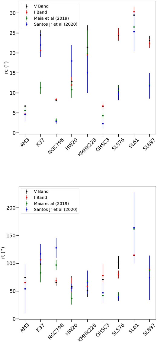
Qualitative comparison of the results found for the structural parameters of the clusters analysed. Top panel shows the core radius and bottom panel shows the tidal radius with their respective uncertainties.
6.1 SL576
As previously mentioned, diffraction patterns and bleeding are not typically accounted for when adding artificial stars to the catalogue instead of the image. In this case, these effects were especially critical for obtaining the structural parameters. Fig. 12 showcases an RGB (red giant branch) image of SL576 composed from SAMI frames where the saturated star is evident.
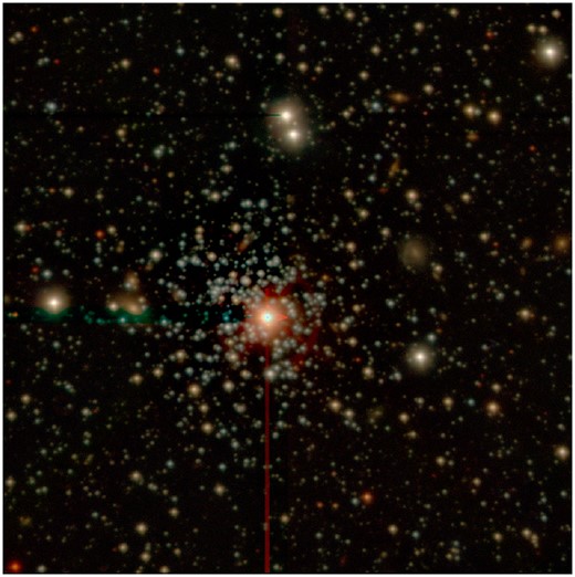
Image of SL576 in the SAMI field of view (3 × 3 arcmin), where we can clearly see the saturated star near the centre of the image. South is up and east to the right.
We created the extended sources masks, as mentioned in Section 3.2. They are displayed in Figs 13 and 14. The bleeding pixels are clearly discernible in the I band.
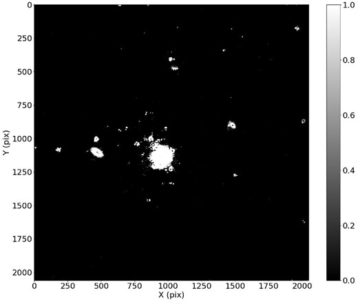
Extended sources mask for SL576 in the V band.
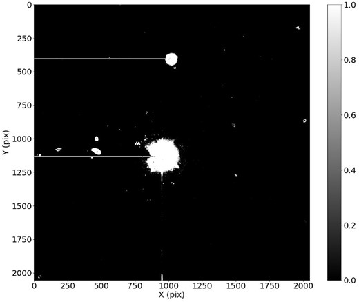
Extended sources mask for SL576 in the I band.
Figs 15 and 16 present the completeness of the catalogued observed stars for this cluster in both V and I bands. We highlighted the region corresponding to the highly saturated star by drawing a circle centred on that star. The effects of saturation are evident in two phenomena: the absence of some stars in the circled region and the low completeness of stars surrounding this area. Completeness curves for this cluster are shown in Fig. B6 in Appendix B.
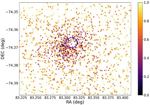
Completeness of stars of SL576 in the V band. Details as in Fig. 5. The blue circle is centred on the position of the highly saturated star near the centre of the cluster.
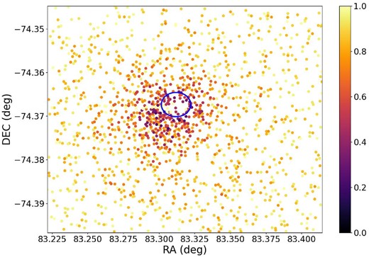
Completeness of stars of SL576 in the I band. Details as in Fig. 15.
For this cluster, Santos et al. (2020) determined |$r_c = 9.7\,\mathrm{ arcsec}$| and |$r_t = 39\,\mathrm{ arcsec}$| using the SBP, while Maia et al. (2019) derived |$r_c = 10\,\mathrm{ arcsec}$| and |$r_t = 43\,\mathrm{ arcsec}$|. Our results for SL576 cluster did not match either of these estimations. However, Santos et al. (2020) found |$r_c = 22\,\mathrm{ arcsec}$| and |$r_t = 148\,\mathrm{ arcsec}$| using a King model fit to the RDP, which aligns more closely with our findings within the uncertainty margin. We also observed discrepancies in our |$r_t$| values between the V and I bands. This may be explained by the significant saturation effect in the I band for this cluster, leading to the recovering of fewer stars in this band, both in the catalogue and in the artificial star grid.
6.2 Discussion
Li et al. (2013) pointed out the influence of saturated stars and diffraction patterns of bright stars on the completeness of HST data. Its worth considering the density differences between the clusters analysed in our study and those in the works of Hu et al. (2011) and Li et al. (2013). Their findings suggest that catalogue based completeness curves in lower density regions align with traditional analysis methods. Even though our sample consists mainly of low-density clusters, we performed the present analysis considering extended sources, which indeed made the completeness estimates more similar to the traditional one.
Our completeness method is not intended to replace the traditional approach. But its estimations reproduces the traditional results with an average margin of error of 10 per cent. The key advantage of our approach is the significant reduction in the time required to perform the entire analysis.
The main purpose of this work is to have good completeness estimates to the entire VISCACHA database, at the moment including images for more than 200 clusters.
7 CONCLUSION AND PERSPECTIVES
Our method takes into account the observational parameters besides the stellar density in each region. Comparing with previous results, our method produces satisfactory results, in general terms. In the sake of the completeness calculations, we reduced the processing time from order of days to 1–2 h to estimate the completeness for the entire 3 × 3 arcmin field of view in a range of 10–15 mag in two different filters when using only the catalogues when compared to the traditional method.
One notable improvement in our methodology is the refinement of the calculation of the background stellar density. This adjustment could further enhance the accuracy of our analysis beyond the current magnitude limit. Additionally, the classification of clusters into only two types, based mainly on their density, was a simplification for the purpose of this study. However, given the vast variety of clusters, a more nuanced classification based on morphology, density of stars, and visual size could provide deeper insights and enable a more comprehensive analysis of their characteristics. Aside from the structural parameters, we might also consider the completeness to analyse the dynamical behaviour of star clusters in a more complex work.
In summary, our study sets the stage for further investigations into the structural properties and dynamics of star clusters. The proposed refinements and extensions have the potential to provide a deeper understanding of the formation and evolution of these clusters within the MCs system.
ACKNOWLEDGEMENTS
We thank the anonymous referee for the suggestions and ideas which helped to improve this manuscript as well as the whole methodology. This research was financed in part by the Coordenação de Aperfeiçoamento de Pessoal de Nível Superior – Brasil (CAPES) – Finance Code 001. It is also partially supported by the Argentinian institution SECYT (Universidad Nacional de Córdoba) and Consejo Nacional de Investigaciones Científicas y Técnicas de la República Argentina, Agencia Nacional de Promoción Científica y Tecnológica. The authors also thank Conselho Nacional de Desenvolvimento Científico e Tecnológico (CNPq). JFG and BPLF acknowledge financial support from CNPq (proc. 141875/2023-2 and 140642/2021-8). FFSM acknowledges financial support from CNPq (proc. 404482/2021-0) and from FAPERJ (proc. E-26/201.386/2022 and E-26/211.475/2021). BD acknowledges support by ANID-FONDECYT iniciación grant no. 11221366 and from the ANID Basal project FB210003. SOS acknowledges FAPESP (proc. 2018/22044-3) and the DGAPA–PAPIIT grant IA103122.
The work is based on observations obtained at the SOAR telescope (projects SO2016B-018, SO2017B-014, CN2018B-012, SO2019B-019, SO2020B-019, and SO2021B-017), which is a joint project of the Ministério da Ciência, Tecnologia, e Inovação (MCTI) da República Federativa do Brasil, the U.S. National Optical Astronomy Observatory (NOAO), the University of North Carolina at Chapel Hill (UNC) and Michigan State University (MSU).
DATA AVAILABILITY
The data underlying this article are available in the NOIRLab Astro Data Archive (https://astroarchive.noirlab.edu/) or upon request to the authors.
REFERENCES
APPENDIX A: DETERMINATION OF FREE PARAMETERS FOR THE AM3 CLUSTER
In this appendix, we present Table A1 displaying the equivalence index |$\xi$| to determine the best combinations of free parameters for the AM3 in both V and I bands. The values of the best combination of free parameters after the entire analysis are highlighted.
Equivalence indices |$\xi$| for AM3 in both bands.
| |$\xi$|V | |$\xi$|I | |||||||
|---|---|---|---|---|---|---|---|---|
| D1 | ||||||||
| dlim | Box | Box | ||||||
| 16 | 25 | 49 | 100 | 16 | 25 | 49 | 100 | |
| 1.0 | 0.038 | 0.033 | 0.023 | 0.021 | 0.051 | 0.048 | 0.041 | 0.040 |
| 1.5 | 0.041 | 0.029 | 0.017 | 0.014 | 0.043 | 0.037 | 0.028 | 0.028 |
| 2.0 | 0.057 | 0.038 | 0.019 | 0.013 | 0.049 | 0.036 | 0.022 | 0.020 |
| 3.0 | 0.091 | 0.077 | 0.040 | 0.025 | 0.078 | 0.062 | 0.027 | 0.017 |
| 4.0 | 0.095 | 0.090 | 0.071 | 0.045 | 0.083 | 0.077 | 0.051 | 0.027 |
| 5.0 | 0.095 | 0.090 | 0.085 | 0.067 | 0.082 | 0.078 | 0.068 | 0.043 |
| D3 | ||||||||
| dlim | Box | Box | ||||||
| 16 | 25 | 49 | 100 | 16 | 25 | 49 | 100 | |
| 1.0 | 0.027 | 0.026 | 0.029 | 0.031 | 0.046 | 0.045 | 0.046 | 0.047 |
| 1.5 | 0.018 | 0.018 | 0.020 | 0.022 | 0.029 | 0.029 | 0.031 | 0.035 |
| 2.0 | 0.016 | 0.014 | 0.016 | 0.018 | 0.021 | 0.021 | 0.023 | 0.027 |
| 3.0 | 0.024 | 0.020 | 0.019 | 0.020 | 0.019 | 0.016 | 0.017 | 0.020 |
| 4.0 | 0.039 | 0.032 | 0.029 | 0.029 | 0.026 | 0.021 | 0.019 | 0.021 |
| 5.0 | 0.056 | 0.047 | 0.041 | 0.040 | 0.037 | 0.028 | 0.024 | 0.025 |
| D5 | ||||||||
| dlim | Box | Box | ||||||
| 16 | 25 | 49 | 100 | 16 | 25 | 49 | 100 | |
| 1.0 | 0.023 | 0.024 | 0.026 | 0.031 | 0.048 | 0.048 | 0.047 | 0.048 |
| 1.5 | 0.019 | 0.018 | 0.020 | 0.025 | 0.034 | 0.034 | 0.036 | 0.038 |
| 2.0 | 0.017 | 0.016 | 0.018 | 0.022 | 0.028 | 0.027 | 0.029 | 0.032 |
| 3.0 | 0.022 | 0.020 | 0.019 | 0.020 | 0.022 | 0.019 | 0.021 | 0.024 |
| 4.0 | 0.036 | 0.031 | 0.029 | 0.028 | 0.023 | 0.020 | 0.020 | 0.022 |
| 5.0 | 0.049 | 0.044 | 0.042 | 0.038 | 0.031 | 0.026 | 0.025 | 0.025 |
APPENDIX B: COMPARISON BETWEEN METHODS
In this appendix, we present a series of figures that demonstrate the comparison between the traditional and our proposed methods of estimating completeness for the remaining clusters. Figs B1–B8 display the completeness curves by both the traditional and our proposed methods and the respective residuals in V and I bands.
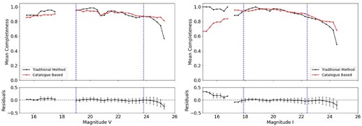
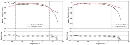
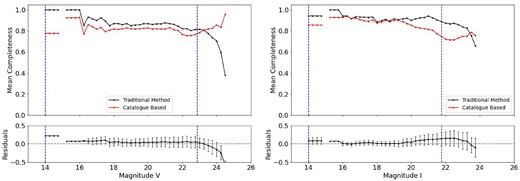
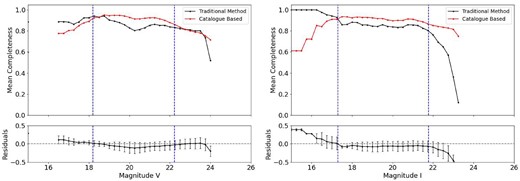
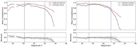
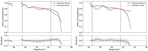
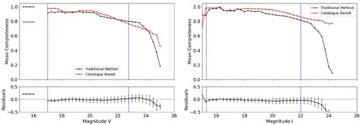
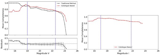
Completeness curves and residuals for SL897 in the both bands. Details as in Fig. 8 for V band. Completeness data for the I band by the traditional method is missing.
APPENDIX C: STRUCTURAL PARAMETERS FOR STUDIED CLUSTERS
In this appendix, we present a compilation of figures resulting from the structural analysis of the studied clusters, as described in Section 5. The figures showcase the fits of the King Function (equation 5) over the RDPs of the clusters for the V and I bands.
Figs C1–C8 depict the fitting of the King Function to the RDPs of clusters in V and I bands. These figures provides a visual representation of the goodness of fit between the theoretical model and the observed density distribution of stars in each cluster. They provide us a comprehensive analysis of the clusters’ structural properties across different wavelengths.
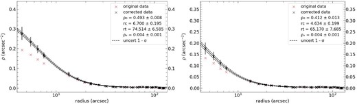
King model fits with 1σ uncertainty to the completeness corrected RDPs of AM3 in V (left panel) and I (right panel). Details as in Fig. 10.
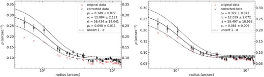
King model fits with 1σ uncertainty to the completeness corrected RDPs of HW20 in V (left panel) and I (right panel). Details as in Fig. 10.
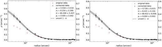
King model fits with 1σ uncertainty to the completeness corrected RDPs of NGC796 in V (left panel) and I (right panel). Details as in Fig. 10.
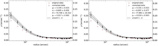
King model fits with 1σ uncertainty to the completeness corrected RDPs of OHSC3 in V (left panel) and I (right panel). Details as in Fig. 10.
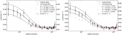
King model fits with 1σ uncertainty to the completeness corrected RDPs of KMHK228 in V (left panel) and I (right panel). Details as in Fig. 10.
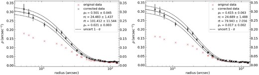
King model fits with 1σ uncertainty to the completeness corrected RDPs of SL576 in V (left panel) and I (right panel). Details as in Fig. 10.
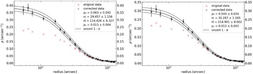
King model fits with 1σ uncertainty to the completeness corrected RDPs of SL61 in V (left panel) and I (right panel). Details as in Fig. 10.
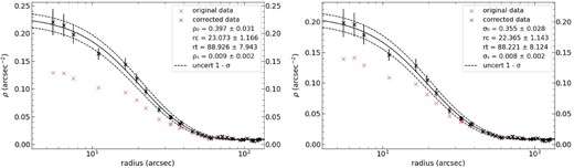
King model fits with 1σ uncertainty to the completeness corrected RDPs of SL897 in V (left panel) and I (right panel). Details as in Fig. 10.
