


ABSTRACT
Cosmological simulations serve as invaluable tools for understanding the Universe. However, the technical complexity and substantial computational resources required to generate such simulations often limit their accessibility within the broader research community. Notable exceptions exist, but most are not suited for simultaneously studying the physics of galaxy formation and cosmic reionization during the first billion years of cosmic history. This is especially relevant now that a fleet of advanced observatories (e.g. James Webb Space Telescope, Nancy Grace Roman Space Telescope, SPHEREx, ELT, SKA) will soon provide an holistic picture of this defining epoch. To bridge this gap, we publicly release all simulation outputs and post-processing products generated within the thesan simulation project at www.thesan-project.com. This project focuses on the z ≥ 5.5 Universe, combining a radiation-hydrodynamics solver (arepo-rt), a well-tested galaxy formation model (IllustrisTNG) and cosmic dust physics to provide a comprehensive view of the Epoch of Reionization. The thesan suite includes 16 distinct simulations, each varying in volume, resolution, and underlying physical models. This paper outlines the unique features of these new simulations, the production and detailed format of the wide range of derived data products, and the process for data retrieval. Finally, as a case study, we compare our simulation data with a number of recent observations from the James Webb Space Telescope, affirming the accuracy and applicability of thesan. The examples also serve as prototypes for how to utilize the released data set to perform comparisons between predictions and observations.
1 INTRODUCTION
Numerical simulations are a fundamental pillar of modern astrophysical research. They represent the most practical approach to solve the equations governing the complex multiscale (astro)physics of galaxy formation in a general and coupled way. Moreover, these simulations enable synthetic experiments that sidestep the inherent limitations of conducting real-world tests on astronomical entities, thereby fulfilling a key aspect of the scientific method within astrophysics.
Recent decades have witnessed the rapid transition from pioneering works employing relatively small-scale, low-resolution dark matter (DM)-only simulations (Press & Schechter 1974; Davis et al. 1985) to significantly more advanced and rigorously validated, large-scale cosmological hydrodynamical simulations (for a recent review of the field see Vogelsberger et al. 2020a). Notable among the latter are: Illustris (Genel et al. 2014; Vogelsberger et al. 2014a, b), Eagle (Schaye et al. 2015), MassiveBlackII (Khandai et al. 2015), Magneticum (Dolag, Komatsu & Sunyaev 2016), Romulus-25 (Tremmel et al. 2017), IllustrisTNG (Marinacci et al. 2018; Naiman et al. 2018; Nelson et al. 2018, 2019; Springel et al. 2018; Pillepich et al. 2018b, 2019), Simba (Davé et al. 2019), NewHorizon (Dubois et al. 2021), FIREBox (Feldmann et al. 2022) and MillenniumTNG (Hernández-Aguayo et al. 2023; Kannan et al. 2023; Pakmor et al. 2023). For the first time, these simulations have achieved a comprehensive and accurate representation description of the observed properties of galaxies over a representative volume and a large fraction of the Universe’s history. They self-consistently follow the evolution of DM and gas, and implement models for the formation and evolution of stellar populations and black holes. However, a common limitation among these simulations is the fact that they all forgo simulating radiation and instead employ a spatially uniform time-evolving radiation field (commonly referred to as UV background, or UVBG in short). While this approximation holds reasonably well in the post-reionization intergalactic medium (IGM) below z ≲ 4.5, it breaks down at higher redshifts as a consequence of the highly spatially inhomogeneous radiation field emitted by localized short-lived sources and with short mean free paths. Additionally, such approximation is never accurate inside and in the vicinity of galaxies, where the radiation from local sources dominates over the background for several tens of kpc.
In recent years, a number of numerical simulations have focused on the Cosmic Dawn and the Epoch of Reionization (EoR). The latter was a pivotal period of time when the radiation emitted by the first stars and galaxies progressively ionized the gas in the IGM between them. Some noteworthy examples in this domain are CROC (Gnedin 2014), CoDa (Ocvirk et al. 2016, 2020; Lewis et al. 2022), AURORA (Pawlik et al. 2017), SPHINX (Rosdahl et al. 2018, 2022), OBELISK (Trebitsch et al. 2021), and Technicolor Dawn (Finlator et al. 2018), each endeavouring to self-consistently incorporate the effect of radiation transport (RT). However, the computational demands imposed by RT often result in limitations, the most common of which are restricted simulation volumes or too coarse of resolutions. In addition, all these runs employ physical models that have been calibrated at the high redshifts investigated (often by matching the observed UV luminosity function) and not as well-studied past z ≲ 5. Furthermore, these simulations typically rely on physical models calibrated for high-redshift phenomena, often validated against observed UV luminosity functions. This raises questions about the model applicability beyond redshifts z < 5 and, consequently, the generalizability of the insights derived from them. For instance, extending the SPHINX galaxy formation model to lower redshift appears to give rise to an excessive number of bulge-dominated galaxies (Mitchell et al. 2021).
To address some of the limitations outlined above, we have developed the thesan suite of radiation-magneto-hydrodynamical (RMHD) cosmological simulations, designed to provide a comprehensive view of the z ≳ 5 reionizing Universe [presented in the three introductory papers: Garaldi et al. (202,2, hereafter Paper i), Kannan et al. (2022,a, hereafter Paper ii), and Smith et al. (2022,a, hereafter Paper iii)]. thesan leverages the well-tested IllustrisTNG galaxy formation model, which has been successful in reproducing the properties of post-reionization galaxies, and complements this with self-consistent RT and cosmic dust modelling. The suite follows a volume large enough to capture the average properties of reionization,1 while also maintaining a resolution adequate to accurately simulate global galaxy properties. It features runs that explore a variety of physical models for the escape of ionizing photons and the nature of DM. Today, thesan stands as one of the most advanced tools available to study the reionizing Universe in a holistic manner, offering reliable predictions across a range of physical quantities related to both galaxies and cosmic reionization. To make the thesan suite an asset to the entire community, we are publicly releasing all of the available raw data and post-processing products. This paper serves as an overview of this data release and aims at providing guidance for practical use.
The practice of publicly releasing large data sets in astronomy has a relatively long history now, both for observational data (starting from the SDSS SkyServer, Szalay et al. 2000) and numerical simulations (e.g. the release of the Millenium simulation by Springel et al. 2005b; Lemson & Virgo Consortium 2006). However, while there has been some initial progress, in the context of EoR simulations the adoption of open data practices remains rare, partially due to resource constraints. This effectively limits their broader utilization and reproducibility. We aim to establish this as standard practice with our data release, which we implement through the accessible and widely used globus2 tool (see Section 4.1). We loosely model the release after the IllustrisTNG (Nelson et al. 2019) one. We offer an online interface to selectively download raw data and post-processed data products, and we provide extensive online documentation and usage examples, and the possibility to import thesan data into popular analysis tools.
Recently, the SPHINX collaboration announced a public data release (Katz et al. 2023). However, at the time of writing, the available data consists of a catalogue containing galaxy properties and synthetic spectra for a sub-sample of 1400 simulated galaxies. We expand significantly on this with our unrestricted data release, allowing downloads of our full snapshot and post-processed data at all output times, providing significant scope for analyses focused on dynamics within individual galaxies all the way up to the science of the IGM.
In this paper, we begin by summarizing the salient properties of the thesan simulations in Section 2. We then provide a thorough description of the released data and associated analysis products in Section 3, including instructions to retrieve them. We discuss some considerations for effective usage in Section 4. Finally, we showcase the predictive power and physical richness of the thesan simulations by providing a few example comparisons with recent James Webb Space Telescope (JWST) observations in Section 5, followed by our summary and conclusions in Section 6.
2 SIMULATION DESCRIPTION
thesan is a state-of-the-art suite of RMHD cosmological simulations, recently developed to provide a holistic view of the early Universe. Specifically, it is designed to simultaneously model the formation of galaxies during the first billion years after the Big Bang, the evolving and spatially inhomogeneous properties of the IGM during Cosmic Dawn and the EoR, and crucially their connection.
To achieve this ambitious objective, thesan combines a large (95.5 cMpc)3 volume with sufficiently high resolution to model the formation of atomic cooling haloes, the smallest structures significantly contributing to the reionization process. thesan simulates a wide range of physical processes relevant to the high-redshift Universe. These include stochastic star formation following the Kennicut-Schmidt relation, magnetic fields, mass, energy and metal return from supernovae (type Ia and II) as well as AGB stars, galactic winds, and black holes (including accretion, bi-modal feedback and radiation output). It also features binary stellar evolution as part of the stellar population synthesis model, explicit tracking of nine metal species (namely H, He, C, N, O, Ne, Mg, Si, Fe), and cosmic dust production, evolution, and destruction. In addition, the ICs for the thesan runs were generated using the variance-suppression technique of Angulo & Pontzen (2016) to boost the statistical significance of box-averaged results.
2.1 Technical details
During the design phase of thesan, we made the explicit decision to utilize physical models that have been calibrated at lower redshifts. thesan is an extension of the IllustrisTNG model (Weinberger et al. 2017; Marinacci et al. 2018; Naiman et al. 2018; Nelson et al. 2018; Pillepich et al. 2018a, b; Springel et al. 2018), specifically tailored to the reionizing Universe. As such, it inherits the core physical framework of IllustrisTNG, with the following key modifications:
The spatially uniform UV background is replaced by self-consistent RT (arepo-rt; Kannan et al. 2019), which follows photons injected from stars and active galactic nuclei (AGN) across three adjacent frequency bins defined by the following photon energy thresholds [13.6, 24.6, 54.4, ∞) eV.
The equilibrium cooling of IllustrisTNG is replaced by a non-equilibrium thermo-chemistry module that simultaneously solves the equations for heating, cooling, and ionization, ensuring that the rapidly evolving reionization fronts can be more faithfully tracked.
A model for cosmic dust production, evolution, and destruction by McKinnon, Torrey & Vogelsberger (2016) and McKinnon et al. (2017) is incorporated, facilitating self-consistent predictions of the dust content of high-z galaxies.
Adopting this approach offers three distinct advantages: (i) It enables the validation of physical models, originally calibrated at z ∼ 0, in the high-redshift regime. (ii) It ensures that the simulations employ a physical model that remains reliable and realistic even beyond the end of the simulations, where it would otherwise be unverifiable.3 (iii) thesan introduces only a single additional free parameter, the unresolved stellar escape fraction, fesc. We calibrate the latter by broadly matching the simulated reionization history to a so-called ‘late reionization’ model (e.g. Kulkarni et al. 2019; Keating et al. 2020), which best fits the latest observations of Ly α effective optical depth at the tail end of reionization (e.g. Zhu, Avestruz & Gnedin 2020; Bosman et al. 2021). The presence of a singular calibration parameter strengthens the comparison between thesan and observational data (as done e.g. in Section 5). This serves as a robust test of the physical model implemented in the simulations, which was primarily developed to reproduce low-redshift observations.
The simulations are performed using the arepo code (Springel 2010; Pakmor et al. 2016; Weinberger, Springel & Pakmor 2020), which solves the magneto-hydrodynamics equations on a mesh, constructed as the Voronoi tessellation of a set of mesh-generating points that follow the gas flow, providing a natural way to enhance resolution in high-density regions. Gravitational forces are calculated using a hybrid TreePM approach, where the long-range part of the gravitational interaction is calculated using a particle-mesh algorithm, while the short-range forces are computed through a hierarchical oct-tree (Barnes & Hut 1986). Radiation is included through the arepo-rt extension (Kannan et al. 2019), which solves the first two moments of the RT equation, supplemented by the M1 closure relation (Levermore 1984), with a manifestly photon-conserving scheme. The number of photons emitted by stars is determined using the BPASS library (Eldridge et al. 2017; Stanway & Eldridge 2018, version 2.1), assuming a Chabrier (2003) initial mass function (IMF) for stars. We assume the radiation emitted by AGN follows the spectral shape of Lusso et al. (2015) rescaled to match the total bolometric luminosity computed from the simulated black hole accretion rate. Please refer to Paper i for further details on the design and calibration of the simulations.
2.2 Numerical setup and available simulations
thesan is composed of one flagship run, designated as thesan-1, which features the highest resolution and implements our fiducial physical model. It is complemented by a series of additional runs, labelled as thesan-...-2), with eight times lower mass resolution exploring different choices for the escape of ionizing photons, the DM model employed, and the numerical convergence of the simulations. In particular, the thesan-low-2 and thesan-high-2 runs are used to investigate the effect of a halo mass-dependent escape fraction of ionizing photons. This is achieved by forcing fesc = 0 in all haloes with mass above and below |$10^{10} \, {\rm M_\odot }$|, respectively. In thesan-sdao-2, cold DM is replaced with the strong dark acoustic oscillations (sDAO; Cyr-Racine et al. 2014) model by replacing the transfer function used in the production of the ICs. thesan-wc-2 provides a run identical to thesan-2 except for the value of fesc, which has been slightly adjusted to compensate the lower star-formation rate density (SFRD) with respect to thesan-1 and achieve the same reionization history. Concerning numerical variations, thesan-tng-2 implements the original IllustisTNG model (i.e. without dust, and with self-consistent RT replaced by a spatially uniform UVBG), and thesan-nort-2 completely neglects radiation. Additionally, we provide two DM-only runs (thesan-dark-1 and thesan-dark-2) at the same resolution of thesan-1 and thesan-2, but evolved all the way to z = 0.
All simulations within the thesan suite follow the evolution of a patch of the Universe with linear size Lbox = 95.5 cMpc, starting from the same ICs (sampled at different resolutions). In thesan-1, the DM and gas mass resolutions are |$m_\mathrm{DM} = 3.12 \times 10^6 \, {\rm M_\odot }$| and |$m_\mathrm{gas} = 5.82 \times 10^5 \, {\rm M_\odot }$|, respectively. This resolution enables us to resolve atomic cooling haloes (the smallest haloes that contribute significantly to reionization) with approximately 50 DM particles. For the thesan-2 series, these mass resolutions are exactly eight times larger. Table 1 provides additional numerical details for each simulation, including their name, box length (Lbox, in cMpc), initial particle number (Nparticles), DM and gas mass resolution (mDM and mgas, respectively, in M⊙), softening length of star and DM particles (ϵ, in ckpc, also corresponding to the minimum softening length for gas particles), minimum physical cell size at z = 5.5 (|$r^\mathrm{min}_\mathrm{cell}$|, in pc), final redshift (zend), subgrid escape fraction of ionizing photons from the birth cloud (if applicable, fesc), and a short description of the unique feature of the simulation compared to the other runs in the table.
Overview of the thesan simulation suite.
| Name | Lbox | Nparticles | mDM | mgas | ϵ | |$r^\mathrm{min}_\mathrm{cell}$| | zend | fesc | Description |
|---|---|---|---|---|---|---|---|---|---|
| [cMpc] | [M⊙] | [M⊙] | [ckpc] | [pc] | |||||
| thesan-1 | 95.5 | 2 × 21003 | 3.12 × 10⁶ | 5.82 × 10⁵ | 2.2 | 10 | 5.5 | 0.37 | Fiducial |
| thesan-2 | 95.5 | 2 × 10503 | 2.49 × 10⁷ | 4.66 × 10⁶ | 4.1 | 35 | 5.5 | 0.37 | Fiducial |
| thesan-wc-2 | 95.5 | 2 × 10503 | 2.49 × 10⁷ | 4.66 × 10⁶ | 4.1 | 33 | 5.5 | 0.43 | Weak convergence of xH i(z) |
| thesan-high-2 | 95.5 | 2 × 10503 | 2.49 × 10⁷ | 4.66 × 10⁶ | 4.1 | 33 | 5.5 | 0.8 | fesc ∝ Mhalo(> 1010) |
| thesan-low-2 | 95.5 | 2 × 10503 | 2.49 × 10⁷ | 4.66 × 10⁶ | 4.1 | 32 | 5.5 | 0.95 | fesc ∝ Mhalo(< 1010) |
| thesan-sdao-2 | 95.5 | 2 × 10503 | 2.49 × 10⁷ | 4.66 × 10⁶ | 4.1 | 33 | 5.5 | 0.55 | sDAO |
| thesan-tng-2 | 95.5 | 2 × 10503 | 2.49 × 10⁷ | 4.66 × 10⁶ | 4.1 | 30 | 5.5 | - | Original TNG model |
| thesan-nort-2 | 95.5 | 2 × 10503 | 2.49 × 10⁷ | 4.66 × 10⁶ | 4.1 | 35 | 5.5 | - | No radiation |
| thesan-dark-1 | 95.5 | 21003 | 3.70 × 10⁶ | - | 2.2 | - | 0.0 | - | DM only |
| thesan-dark-2 | 95.5 | 10503 | 2.96 × 10⁷ | - | 4.1 | - | 0.0 | - | DM only |
| thesan-hr-res8x | 5.9 | 2 × 5123 | 6.03 × 10⁴ | 1.13 × 10⁴ | 0.425 | 8 | 5.0 | 0.37 | Fiducial |
| thesan-hr | 5.9 | 2 × 2563 | 4.82 × 10⁵ | 9.04 × 10⁴ | 0.85 | 32 | 5.0 | 0.37 | Fiducial |
| thesan-hr-large | 11.8 | 2 × 5123 | 4.82 × 10⁵ | 9.04 × 10⁴ | 0.85 | 15 | 5.0 | 0.37 | Fiducial |
| thesan-hr-sdao | 5.9 | 2 × 2563 | 4.82 × 10⁵ | 9.04 × 10⁴ | 0.85 | 33 | 5.0 | 0.37 | sDAO |
| thesan-hr-wdm | 5.9 | 2 × 2563 | 4.82 × 10⁵ | 9.04 × 10⁴ | 0.85 | 28 | 5.0 | 0.37 | Warm DM (|$3\, {\rm keV}$|) |
| thesan-hr-fdm | 5.9 | 2 × 2563 | 4.82 × 10⁵ | 9.04 × 10⁴ | 0.85 | 23 | 5.0 | 0.37 | Fuzzy DM (|$2\times 10^{-21}\, {\rm eV}$|) |
The columns, from left to right, represent the following attributes: the name of the simulation, linear size of the simulation box, (initial) particle number, mass of DM and gas particles, (minimum) softening length for (gas) star and DM particles, minimum physical cell size at z = 5.5, final redshift, escape fraction of ionizing photons from the birth cloud (if applicable), and a short description of the simulation.
The numbers reported in Table 1 are placed into the broader context of the community effort to simulate the reionizing Universe in Fig. 1, where we compare the force resolution and the simulated volume of the different simulations in the thesan project to those of other radiation hydrodynamic simulations designed to model the formation and evolution of structures at high redshift, namely CROC (Gnedin 2014), CoDa (Ocvirk et al. 2016, 2020; Lewis et al. 2022), SPHINX (Rosdahl et al. 2018, 2022), OBELISK (Trebitsch et al. 2021), Aurora (Pawlik et al. 2017), TechnicolorDawn (Finlator et al. 2018), Renaissance (Xu et al. 2016), Phoenix (Wells & Norman 2022), and SPICE (Bhagwat et al. 2023). For some of them, we have highlighted peculiarities that set them apart from the others in the same group. This emphasizes how the plotted quantities are only two of the many that might characterize a simulation. These simulations range from high-resolution small-volume simulations designed to study the formation of first stars, like the Renaissance and Phoenix simulations, to lower-resolution but large-scale simulations that model a large representative volume of the Universe, namely CROC, CoDa, and thesan. These large volumes are necessary to obtain converged reionization histories and rigorous large-scale IGM predictions (Iliev et al. 2014; Gnedin & Madau 2022). In contrast, the smaller volume calculations primarily serve as galaxy formation simulations with coupled RT rather than comprehensive reionization simulations. Another advantage of the thesan simulations is that they use a well-tested galaxy formation model that has been shown to reproduce realistic galaxy properties down to redshift zero (Springel et al. 2018). In contrast, some other simulations use galaxy formation models that have been designed primarily for higher redshifts. When these galaxy formation models are used to simulate galaxies down to lower redshifts, they give rise to galaxy populations that are incompatible with observations. An example is the model used in SPHNIX and Obelisk, which produces galaxies with much higher stellar masses than observed, that are bugle-dominated, and have centrally peaked rotation curves (Mitchell et al. 2021). These drawbacks make it difficult to assess the accuracy of certain predictions like the LyC production rate and emission line properties, which might be overestimated due to the high stellar masses, and the escape fraction of ionizing photons, which might be underestimated due to inefficient stellar feedback (Trebitsch, Volonteri & Dubois 2020). Therefore, the thesan simulations offer a distinctively comprehensive and reliable approach to the simultaneous study of structure formation and reionization at high redshift.
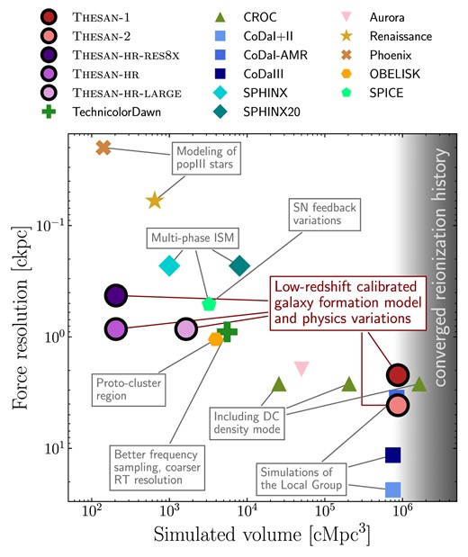
Overview of simulated volume and force resolution of R(M)HD simulations. For some of them we have highlighted peculiarities that set them apart from otherwise similar runs. For grid-based codes, when not otherwise indicated by the authors, we consider the force resolution to be equal to three times the smallest grid cell size. The background grey shading indicates simulation volumes large enough to produce a converged reionization history, making them reliable for reionization studies. The colour gradient reflects the range of volumes required according to different studies (Iliev et al. 2014; Gnedin & Madau 2022).
2.3 Thesan-HR
The thesan suite has been recently augmented with a specialized set of higher-resolution, small-box simulations, designated as thesan-hr. These runs are designed to study in detail the impact of inhomogeneous radiation propagation on smaller haloes. This is carried out both within the framework of the standard ΛCDM cosmology (Borrow et al. 2023) and in beyond-CDM models (Shen et al. 2024). We release the data for these runs alongside the main thesan boxes, and include them in both Table 1 and Fig. 1 for catalogue and visual representations.
2.4 Overview of the first results
The thesan suite has already produced a number of scientific results. We summarize here those that could potentially impact future applications of the data. Specifically, we have calibrated the birth cloud escape fraction of ionizing photons (fesc) to align with a late reionization history in thesan-1. This calibrated value is consistently applied across thesan-2 and thesan-sdao-2. In thesan-wc-2, the value has been fine-tuned to match the reionization history of thesan-1. For thesan-low-2 and thesan-high-2, it has been re-calibrated due to their modified mechanisms for the escape of ionizing photons. This procedure results in all of the thesan runs reaching a volume-weighted4 hydrogen ionized fraction of 99 per cent by z ≲ 5.8, with thesan-1 reaching this value at z ≈ 5.5 (see fig. 3 of Paper ii). The only exception is thesan-low-2, which completes reionization much earlier (approximately at z ≈ 6.6) as a result of the enhanced contribution from low-mass galaxies that dominate at higher redshifts.
thesan exhibits strong agreement with observed stellar-to-halo-mass relations and stellar mass functions at 6 ≤ z ≤ 10 (see figs 9 and 10 of Paper i). It also aligns well with the high-redshift UV luminosity function over the same redshift range (UVLF; fig. 11 of Paper i). This is remarkable, as this quantity is typically calibrated against in reionization-era simulations. It should be noted, however, that to reach such an agreement it is necessary to adopt the dust attenuation relation developed for IllustrisTNG in Vogelsberger et al. (2020b). Using the self-consistently simulated dust masses, the bright end of the UVLF is not attenuated enough, suggesting a potential under-production of dust in thesan. Unfortunately, observations in the same stellar mass range only provide upper limits on the total dust mass (see fig. 15 of Paper i). The metal production, however, is in excellent agreement with the observed mass–metallicity relation (see fig. 14 of Paper i).
The IGM in thesan shows a realistic broad distribution in the temperature-density space, both during and after reionization (see fig. 4 of Paper ii). Key metrics such as the H i photo-ionization rate in ionized regions, the mean free path of ionizing photons, and the CMB optical depth are in excellent agreement with existing data (see figs 5, 7, and 3 of Paper ii, respectively). However, the Ly α mean transmitted flux and effective optical depths distribution consistently indicate that a slightly later reionization is preferred (see figs 9 and 11 of Paper ii). While fig. 2 of Paper ii might appear to indicate the opposite, we caution the reader that the observational values of xH i at the tail-end of reionization are typically derived by mapping the observed Ly α flux to H i fractions through simulations employing cruder approximations than thesan. Therefore, we consider a comparison with the Ly α flux a more direct test of our model, and trust the conclusion drawn from it more than those from a comparison of the simulated and observationally inferred xH i. Finally, thesan is the first simulation of its kind to reproduce the excess transmitted flux in proximity of galaxies in the Ly α forest of high-redshift quasar spectra (see fig. 15 of Paper ii).
The thesan suite has also been used to study the production of Ly α photons and their transmission through the CGM of galaxies (Paper iii), to provide predictions for forthcoming intensity mapping experiments (Kannan et al. 2022b), to study the escape of ionizing photons from galaxies (Yeh et al. 2023), to calibrate effective field theory models and predict the 21-cm signal of neutral hydrogen (Qin et al. 2022), to study the Ly α emitter luminosity function (Xu et al. 2023), to deepen the understanding of how a UV background influences galaxy properties (Borrow et al. 2023), to predict high-redshift observables in beyond-CDM models (Shen et al. 2024), to compare the evolution of the ionized bubble size to available observations (Neyer et al. 2023), to investigate the evolution of galaxy sizes (Shen et al. 2024) and – combined with the IllustrisTNG and MilleniumTNG runs – to provide predictions of the z ≳ 6 galaxy properties over a wide range of scales (Kannan et al. 2023). All these studies are based on the data that we are publicly releasing alongside this paper, and will we describe in detail in the following sections.
3 DATA AND DATA PRODUCTS
With this paper, we release all the raw data and many post-processing products generated within the thesan suite until now, amounting to nearly 400 terabytes. We plan to release additional data products in the future, as they become available. Current and future data can be found online at https://thesan-project.com, alongside with their complete documentation. At the time of this first data release, we offer the following data and derived products:
Snapshots (Section 3.1): Full simulation output at 80 different cosmic times, between z = 20 and z = 5.5 (produced approximately every 11 Myr).
Group catalogues (Section 3.2): Properties of haloes and galaxies in the simulation, at the same 80 cosmic times of the snapshots.
Cartesian outputs (Section 3.3): Gas properties sampled on a Cartesian grid at high time cadence (approximately every 2.8 Myr).
Simulation.hdf5 file (Section 3.4): Utility file linking together chunked data sets of the simulation;
Merger trees (Section 3.5): Evolutionary tracks of subhaloes and galaxies in the simulation and their properties.
Offset files (Section 3.6): Utility files to simplify the navigation of snapshot, groups and merger trees.
Hashtables (Section 3.7): Utility files to simplify the selection and loading of particles based on their spatial position.
Cross-link files (Section 3.8): Utility files to simplify the identification of ‘twin’ haloes across the different thesan simulations.
Lya catalogues (Section 3.9): Ly α properties of galaxies in the simulations.
Lines of sight (Section 3.10): Collection of gas properties along random lines of sight through the simulation.
Filament catalogues (Section 3.11): Filaments identified in the simulation and their properties.
Escape fraction catalogues (Section 3.12): Escape fraction properties of galaxies in the simulation.
Galaxy SED catalogues (Section 3.13): Synthetic SEDs for well-resolved, star-forming galaxies.
In the subsequent subsections, we briefly describe each data product. For each, we specify two key attributes: a template file name and a list of runs for which the data are available. It should be noted that not all data products are applicable to every thesan run. Table 2 shows which data are available for each individual run. In the remainder of this Section, we use the following naming convention: NNN represents the snapshot number, zero-padded on the left to have exactly three digits, while C denotes the unpadded chunk number.
Overview of the available data and data products for each of the thesan simulations.
| Name | Snapshots | Cartesian | Merger | Offsets | Hashtables | SED | Filaments | Catalogues | ||||
|---|---|---|---|---|---|---|---|---|---|---|---|---|
| outputs | trees | Groups | Ly α | cross-link | LOS | fesc | ||||||
| thesan-1 | ✓ | ✓ | ✓ | ✓ | ✓ | ✓ | ✓ | ✓ | ✓ | ✓ | ✓ | ✓ |
| thesan-2 | ✓ | ✓ | ✓ | ✓ | ✓ | ✗ | ✓ | ✓ | ✓ | ✓ | ✓ | ✓ |
| thesan-wc-2 | ✓ | ✓ | ✓ | ✓ | ✓ | ✗ | ✓ | ✓ | ✓ | ✓ | ✓ | ✓ |
| thesan-high-2 | ✓ | ✓ | ✓ | ✓ | ✓ | ✗ | ✓ | ✓ | ✓ | ✓ | ✓ | ✓ |
| thesan-low-2 | ✓ | ✓ | ✓ | ✓ | ✓ | ✗ | ✓ | ✓ | ✓ | ✓ | ✓ | ✓ |
| thesan-sdao-2 | ✓ | ✓ | ✓ | ✓ | ✓ | ✗ | ✓ | ✓ | ✓ | ✓ | ✓ | ✓ |
| thesan-tng-2 | ✓ | ✗ | ✓ | ✓ | ✓ | ✗ | ✓ | ✓ | ✗ | ✓ | ✓ | ✗ |
| thesan-nort-2 | ✓ | ✗ | ✓ | ✓ | ✓ | ✗ | ✓ | ✓ | ✗ | ✓ | ✓ | ✗ |
| thesan-dark-1 | ✓ | ✗ | ✓ | ✓ | ✗ | ✗ | ✗ | ✓ | ✗ | ✓ | ✗ | ✗ |
| thesan-dark-2 | ✓ | ✗ | ✓ | ✓ | ✓ | ✗ | ✗ | ✓ | ✗ | ✓ | ✗ | ✗ |
| thesan-hr-res8x | ✓ | ✗ | ✗ | ✓ | ✗ | ✗ | ✗ | ✓ | ✓ | ✗ | ✗ | ✓ |
| thesan-hr | ✓ | ✗ | ✓ | ✓ | ✗ | ✗ | ✗ | ✓ | ✓ | ✗ | ✗ | ✓ |
| thesan-hr-large | ✓ | ✗ | ✓ | ✓ | ✗ | ✗ | ✗ | ✓ | ✓ | ✗ | ✗ | ✓ |
| thesan-hr-sdao | ✓ | ✗ | ✗ | ✓ | ✗ | ✗ | ✗ | ✓ | ✓ | ✗ | ✗ | ✓ |
| thesan-hr-wdm | ✓ | ✗ | ✗ | ✓ | ✗ | ✗ | ✗ | ✓ | ✓ | ✗ | ✗ | ✓ |
| thesan-hr-fdm | ✓ | ✗ | ✗ | ✓ | ✗ | ✗ | ✗ | ✓ | ✓ | ✗ | ✗ | ✓ |
For each simulation indicated in the first column, a ✓ indicates that the data product referenced in the corresponding column is available, while a ✗ signifies that these data are not available. The data products are thoroughly described in Section 3. In the future, more data will be made publicly available.
In Fig. 2, we provide an overview of the breadth of the data released. In the central panel (b) we feature a 3D visualization of simulated haloes (grey points, with transparency proportional to their total mass) within the redshift range 5.5 ≤ z ≤ 20 in the thesan-1 simulation box (outlined by black lines). The output times for snapshots and Cartesian outputs are marked along the redshift axis using blue points and yellow bars, respectively. Additionally, cosmic filaments identified in the simulation are depicted with green lines, while the simulated IGM transmissivity to the Ly α line along a random sightline is represented in brown, and a cross-sectional slice through the simulation in orange. In panel (a) we show a number of quantities computed along this slice using Cartesian outputs and synthetic SEDs. Examples of the latter are also shown in Panel (c), along with synthetic JWST images of the corresponding simulated galaxies (generated using the skirt code; see Section 3.13) and the profile of the escaping Ly α line, where the null velocity offset corresponds to the intrinsic galaxy redshift. Panel (d) presents the reionization redshift computed for different runs of the original thesan series along a slice through the simulation volume. Lastly, panels (e) and (f) illustrate, respectively, the escape fraction of ionizing photons at 100 ckpc from the central galaxy and the merger tree for the largest halo in the thesan-1 box. In the merger tree, each progenitor is represented by a circle, the size of which is proportional to its mass, and the colour indicates the reionization state of its environment, defined as a 1 cMpc sphere around it.
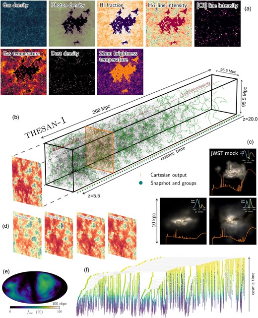
Schematic overview of select data products released with this paper and showing their interconnection. Panel (b) features a lightcone-like 3D rendering of the thesan-1 simulation box in the redshift range 5.5 ≤ z ≤ 20. The simulation box is outlined by black lines, and the output times for full snapshots (see Section 3.1) and Cartesian outputs (see Section 3.3) are indicated in the bottom right of the panel using blue points and yellow bars, respectively. Grey points within the 3D rendering represent simulated haloes (see Section 3.2). We overplot in green the identified filaments (see Section 3.11), in brown the IGM transmissivity to the Ly α line along a random sightline (see Section 3.10), and in orange a slice through the simulation. In panel (a) we show a selection of simulated physical quantities, indicated in the top left of each slice. In panel (c) we show synthetic JWST images and SEDs (background and orange line, respectively, see Section 3.13) of three randomly selected galaxies at z = 6. Panel (d) shows the reionization redshift computed for the different runs of the original thesan series. Finally, panels (e) and (f) show, respectively, the escape fraction of ionized photons (see Section 3.12) at 100 ckpc from the central galaxy and the merger tree (see Section 3.5) for the largest halo in the thesan-1 box. In the latter, each progenitor is shown using a circle of size proportional to its mass and colour proportional to the reionization state of its environment (defined as a 1 cMpc sphere around it).
Comparison with IllustrisTNG data. The data structure for snapshots, group catalogues, merger trees, and offset files are mostly identical in format to those of the IllustrisTNG simulation, allowing the tools developed for these simulations to be used for thesan as well. However, the additional physics simulated in thesan necessitates the inclusion of further physical quantities, mainly related to radiation and cosmic dust. We also introduce an additional output type, named Cartesian output (see Section 3.3). Conversely, some physical quantities have been omitted from the output, as they are not pertinent to the redshift range covered by thesan. We highlight new or modified data fields in the accompanying documentation.
3.1 Snapshots
File name: snapshot_NNN/snap_NNN.C.hdf5
Availability: all runs
Snapshots contain the most complete description available of the simulation. They host a large number of properties for each resolution element (gas, DM, stars, and black holes) in the simulation. Each snapshot provides a record of the simulation at a given cosmic time. thesan provides 80 of these snapshots, approximately every 11 Myr, between z = 20 and z = 5.5 (the exact output times can be found in the thesan website).
Snapshots are stored using the HDF5 file format. Because of their size, each snapshot is split into a number of chunk files, identical in structure, containing only a portion of the complete data set. The organisation of a single snapshot is shown in Fig. 3 and described in the following. Within the snapshot files, particles are divided by type, each one representing different physical components as listed in Table 3 and saved in a different HDF5 group named PartTypeP, where P is an integer. Within each particle group, particles are sorted according to the FoF group (see Section 3.2) they belong to. This means that all the particles belonging to the FoF group 0 are first, followed by those part of the FoF group 1, and so on. Particles not belonging to any FoF group are last, in the so-called ‘outer fuzz’. Within each FoF group, particles are sorted according to their subhalo (as identified by SUBFIND). Particles not associated to any subhalo are last within the group (the so-called ‘inner fuzz’). Finally, within each subhalo, particles are sorted according to their binding energy, from the most bound to the least bound.5 Once these particle lists containing all particles in the simulations have been built, they are split at arbitrary points and stored in separate chunk files. The splitting is performed in such a way to have approximately the same number of resolution elements in each chunk file. As Fig. 3 shows, if a subhalo (of a FOF group) does not contain particles of a given type, it will simply be skipped. Additionally, there is no guarantee that particles of the same subhalo (of a FOF group) will be stored in the same chunk, or that all the particles of a given type of a subhalo will be stored in the same chunk. Finally, chunks are not guaranteed to contain all particle types. If a particle type is absent in a chunk (as PartType5 in chunk 1 in the figure), the corresponding HDF5 group will not be present in the file.
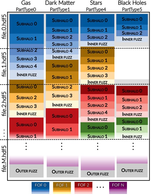
Schematic example of the organization of the thesan snapshot files. Different colours represent each of the different N FOF groups identified in the simulation. Each row shows a different one of the M total file chunks, with each column representing one of the four different particle types.
Correspondence between particle types and the physical components they simulate.
| PartType | Component |
|---|---|
| 0 | Gas |
| 1 | DM |
| 4 | Stars and wind particles |
| 5 | Black holes |
| PartType | Component |
|---|---|
| 0 | Gas |
| 1 | DM |
| 4 | Stars and wind particles |
| 5 | Black holes |
Particle types 2 and 3 are not used in thesan.
Within each PartTypeP HDF5-group, a number of HDF5 data sets are stored, each one corresponding to a different quantity [e.g. position, mass, star-formation rate (SFR)] associated with the resolution elements. The ordering of the particle/cells is the same across these data sets, in such a way that the i-th item of each data set always corresponds to the i-th resolution element. A list and description of available data sets are provided on the thesan website. Each data set contains some attributes that describe the physical quantity stored in the data set and how it scales with the units of the simulation. Finally, each chunk file contains a header group, whose attributes contain general information about the simulation setup, the current snapshot and the current chunk file (also documented on the thesan website).
Note that the snapshots contain a number of new quantities not present in IllustrisTNG, that we list and briefly describe in Table 4, while some other fields have been dropped, as they are either irrelevant for the redshift covered by thesan or too memory-consuming. Of particular relevance for the science case of thesan are the ionized fractions of hydrogen and helium, denoted as HI_Fraction, HeI_Fraction, and HeII_Fraction). These are calculated through the non-equilibrium thermochemistry solver fully coupled with the RT scheme, as opposed to relying on an approximate spatially uniform UV background. Similarly, thesan provides the photon number density across the three frequency bins tracked (see Section 2), which is stored in the PhotonDensity data set in units of |$10^{63} \, (\mathrm{ckpc}\, h)^{-3}$|. Lastly, the GFM_DustMetallicity data set contains the dust-to-gas mass ratio given by the on-the-fly dust model.
New and modified data sets (with respect to IllustrisTNG) stored in the thesan snapshots, sorted by particle type.
| Data set | Units | Description | |
|---|---|---|---|
| PartType0 | GFM_DustMetallicity | - | New. Dust-to-gas ratio of gas cell. |
| GFM_Metallicity | - | Modified. It now includes metals locked in dust. | |
| GFM_Metals | - | Modified. It now includes metals locked in dust. Untracked metals are not stored. | |
| HI_Fraction | - | New. H i fraction of the cells. | |
| HeI_Fraction | - | New. He i fraction of the cells. | |
| HeII_Fraction | - | New. He ii fraction of the cells. | |
| PhotonDensity | 10−63h3 kpc−3 | New. Density of photons in the gas cell in each spectral band. | |
| PartType4 | BirthDensity | 1010 M⊙ h2 ckpc−3 | New. Comoving mass density where this star particle initially formed. |
| GFM_DustMetallicity | - | New. Dust-to-gas ratio of the stellar particle, inherited from the parent gas cell and never changed. | |
| GFM_Metallicity | - | Modified. It now includes metals locked in dust. | |
| GFM_Metals | - | Modified. It now includes metals locked in dust. Untracked metals are not stored. | |
| PartType5 | BH_MPB_CumEgyHigh | 1010 M⊙ h−1 ckpc2/(0.978 Gyr) | New. Cumulative amount of kinetic AGN feedback energy injected into surrounding gas in the high accretion-state (quasar) mode along the main progenitor branch of the black hole merger tree. |
| BH_MPB_CumEgyLow | 1010 M⊙ h−1 ckpc2/(0.978 Gyr) | New. Cumulative amount of kinetic AGN feedback energy injected into surrounding gas in the low accretion-state (wind) mode along the main progenitor branch of the black hole merger tree. | |
| BH_PhotonHsml | h−1 ckpc | New. Comoving radius enclosing 64 ± 4 nearest gas cells, used for photon injection. |
3.2 Halo and subhalo catalogues
File name: groups_NNN/fof_subhalo_tab_NNN.C.hdf5
Availability: all runs
Whenever a snapshot is produced, we also produce halo (i.e. FoF groups) and subhalo (i.e. SUBFIND subgroups) catalogues, identified on-the-fly using the FOF and SUBFIND algorithms (Springel et al. 2001), respectively. The former identifies groups based on spatially close DM particles, while the latter determines groups of physically bound particles. Briefly, the FOF algorithm isolates groups (haloes) of DM particles that are closer than 0.2 times the mean inter-particle distance. Non-DM particles are then associated with the group that contains their nearest DM particle. This subdivision is purely geometrical and does not consider any further physical property of the involved particles and cells. Each of these groups is subsequently split into gravitationally bound systems (subhaloes) using the SUBFIND algorithm.
The group catalogues contain a list of identified haloes and subhaloes (stored in the same file, but contained in the Group and Subhalo HDF5-groups, respectively), and their associated properties (stored in separate HDF5-data sets within the corresponding HDF5-group). Similarly to snapshots, these catalogues are split across a number of chunks and are stored using the HDF5 data format. The former are ranked by DM mass (from the most massive to the least massive one), while subhaloes are ranked by parent group first, and then by DM mass within each parent group.
3.3 Cartesian outputs
File name: cartesian_NNN/cartesian_NNN.C.hdf5
Availability: all RMHD runs except the thesan-hr series
thesan provides a new type of output with respect to IllustrisTNG. Specifically, we save selected gas quantities on a regular Cartesian grid with high time cadence, using a first-order Particle-In-Cell binning approach. thesan-1 uses a 10243 grid while the thesan-2 runs use 5123 grids, setting the cell sizes to ∼93 and ∼186 ckpc, respectively. Cartesian outputs are not available for the thesan-hr runs. The three-dimensional grid is flattened into a C-ordered array (with the z-axis increasing fastest) and then split into chunks, each saved in a different HDF5 file. Each chunk file also stores information as HDF5 attributes of its ‘Header’ HDF5 group, with full details given in the online documentation. While most of the quantities are deposited on a regular spatial grid, some observables (e.g. the 21 cm emission) are binned in redshift space, accounting for Doppler shifting due to the peculiar velocity of individual gas cells. This redshift-space binning is carried out assuming the observed direction is aligned with the + z axis. The Cartesian outputs are written every ∼2.8 Myr amounting to about 400 snapshots over the duration of the simulation. These lower-resolution higher-time-cadence outputs are ideal for studying the large-scale properties of the reionization process.
3.4 The simulation.hdf5 file
File name: simulation.hdf5
Availability: all runs
Similar to IllustrisTNG, we produce a ‘summary’ file named simulation.hdf5 for each simulation, placed in its root directory. This file employs HDF5 virtual data sets to link all halo and subhalo catalogue fields, snapshot particle fields, individual snapshot headers and Cartesian outputs in a single file of limited size. In addition, it also contains configuration flags and parameters of the simulation. Because of its nature, this file requires that all files linked (namely group, snapshot, Cartesian, and offsets files) to be downloaded and placed in the same directory structure. This file is completely optional and provided only for convenience.
The simulation.hdf5 file hides the division of (some) outputs into chunks. In fact, through this file it is possible to index fields as if they were not split among file chunks. The virtual data sets take care of loading the requested values from the file chunks and joining them together.
3.5 Merger trees
File name: trees_sf1_080.C.hdf5
Availability: all runs except the thesan-hr non-ΛCDM ones
We provide merger trees describing the build-up of haloes over cosmic time. These are built using the LHaloTree code (Springel, Di Matteo & Hernquist 2005a) and are named trees_sf1_080.C.hdf5, where C is the chunk number (without padding). In short, to determine the appropriate descendant, the unique IDs that label DM particles are tracked between outputs. For a given halo, the algorithm finds all haloes in the subsequent output that contain some of its particles. These are then counted in a weighted fashion, giving higher weight to particles that are more tightly bound in the halo under consideration, and the one with the highest count is selected as the descendant. In this way, preference is given to tracking the fate of the inner parts of a structure, which may survive for a long time upon infall into a bigger halo, even though much of the mass in the outer parts can be quickly stripped. To allow for the possibility that haloes may temporarily disappear for one snapshot, the process is repeated for snapshot n to snapshot n + 2. If either there is a descendant found in snapshot n + 2 but none found in snapshot n + 1, or, if the descendant in snapshot n + 1 has several direct progenitors and the descendant in snapshot n + 2 has only one, then a link is made that skips the intervening snapshot.
The merger tree structure is split across a number of HDF5 files and, within each file, in a number of TreeX groups. For each halo across all snapshots, there is one entry in this structure. Haloes are linked together in branches, describing which progenitor haloes have merged to create a descendant one. Each entry of the tree structure contains a link to the descendant (i.e. the halo it contributed the most particles in the subsequent snapshot), the next progenitor (i.e. the next item in the list of progenitors at the same redshift that contributed to the descendant halo) and its first progenitor (i.e. the most massive halo in the list of its progenitor in the previous snapshot). They also contain a number of subhalo properties inherited from the group catalogue that are stored in these files for ease of access.
3.6 Offset files
File name: offsets_NNN.hdf5
Availability: all runs
The ordering of particles in the snapshots as well as the large number of particles and haloes in the simulation render it sometimes inconvenient or slow to load specific particles, haloes or merger tree entries. To ease this task, we produced so-called offset files, designed to allow an easy navigation between other data products. There is one such file for each snapshot of each simulation. These files provide a mapping between halo or particle indices and their memory position (i.e. chunk file and position within it), as well as a mapping between the halo number and position in the merger tree structures (identified as a combination of chunk number, tree number and index within the tree). The offset files provide also the inverse mapping, from chunk file to the range of particles or groups contained.
The thesan website contains a thorough description of available fields in these files. Practically speaking, in order to, e.g., load the gas particles of the subhalo with global index j from the simulation snapshots, one can simply:
load the offset file for the relevant redshift,
index the HDF5 data set Subhalo/SnapByType with the index j to obtain the global index k of the first gas particle of the subhalo,
index the HDF5 data set FileOffsets/SnapByType with the index k to obtain the chunk number n storing the particle,
load the appropriate chunk file n and load the subhalo gas particles, potentially continuing from the following chunk file (n + 1) if the chunk file n contains less gas particles than belonging to the subhalo (as indicated by the Subhalo/SubhaloLenType HDF5 data set in the group catalogue).
We provide utility python functions to perform this and other tasks on the thesan website.
3.7 Hashtables
File name: spatial_hashtable_NNN.hdf5
Availability: all runs except the thesan-hr series
As described in Section 3.1, particles are sorted in the snapshots based on the FoF group to which they belong, with particles not assigned to any halo stored at the end. Selecting particles based on their spatial location (as necessary for e.g. studies of the CGM and IGM surrounding galaxies) necessitates loading the entire coordinate list of the particles of this type, which is both wasteful and not possible on all machines due to memory constraints, while loading chunk after chunk can be very slow. In order to circumvent this issue, we provide hashtable files, created using the sparepo6python module. These files and the associated module allow users to read snapshots based upon the spatial volume requested, rather than by galaxy or halo number, in a coarse-grained way.
The structure of the files and their application to real data is demonstrated in Fig. 4, where we show a single ‘cell’ from the spatial hashtable, with particles assigned to the cell represented as points (coloured by the file they were read from). The files themselves are designed to be both human and machine readable, with fast routines (accelerated with numba) implemented in sparepo to read the data. sparepo can additionally provide extra utility, such as reading the data with symbolic units leveraging the unyt package.
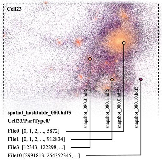
A demonstration of the spatial hashtable applied to thesan data. Each point represents one gas (particle type 0) particle, with the points coloured by the sub-snapshot that they were read from. The diagram at the bottom of the figure shows how the spatial hashtable file is structured.
The files are structured as follows: for every snapshot there is a spatial hashtable file. Within the file, there are metadata describing the cell layout (read automatically by sparepo; see the documentation for a full description of these metadata), which is a Cartesian grid with 20 cells per axis (8000 cells per file), meaning each cell has a volume of roughly (5 cMpc)3. This cell size was chosen to optimise both data storage volumes and reading times. For each cell in the volume, there is an independent data group named CellX (with X being a unique cell ID as described by the metadata), each containing (up to) four particle type data groups named PartTypeP, identical to the snapshots. Within each of these lowest level of groups, there are data sets named FileC, where C is the file chunk that contributes particles of this type to the cell. The FileC data sets contain a sorted array of 32 bit integers referring to the index within the chunk file (C) that particles residing within this chunk inhabit. This makes it possible to load the relevant chunks for a specific position (and search radius) within the volume to read both galaxies within the chunk and all associated ‘fluff’ (i.e. the IGM). This significantly smaller array of particle properties can then be further filtered. Documentation and usage examples of these files can be found on the sparepo website.
3.8 Cross-link files
File name: cross_link.hdf5
Availability: all runs except the thesan-hr series
One of the highlight features of the thesan simulation suite is the inclusion of multiple runs with different physical models for the escape of ionizing photons and for the nature of DM. In order to enable a one-to-one comparison between objects in the different runs, we provide cross-matched catalogues linking the subhaloes at a given redshift across different runs. They were built following the same approach as the merger trees (i.e. maximizing the weighted number particles shared between two subhaloes), except that instead of linking subhaloes across snapshots we link them across simulation runs. For each simulation run we provide a file named cross_link.hdf5, which contains an HDF5 group for each other run at the same resolution. Within each group, there is a data set for each snapshot containing a list of IDs. The value in position j is the subhalo global index of the object associated in the other simulation (specified by the HDF5 group) with subhalo of global index j in the current simulation. More transparently, for a simulation SIM1, the subhalo of global index j is paired to the one in SIM2 of global index given by the HDF5 data set to_SIM2/snap_NNN[j], where NNN has the usual meaning.
There is no guarantee that subhaloes are bijectively and unequivocally associated in two simulations; i.e. it is possible that the subhalo j1 in SIM1 is associated with subhalo j2 in SIM2, but the latter is not associated with subhalo j1 in SIM1. Moreover, it is also possible that a single halo in one run is associated to multiple haloes in another one. Finally, it is possible that no association is found, in which case the cross-link will have the value -1. These cases represent a minority (typically below 5 per cent of the total), arising both for physical and numerical reasons, e.g. due to a different power spectrum in the ICs, slightly different output times in different simulations, and random variability between simulations (see e.g. Genel et al. 2019; Keller et al. 2019; Borrow et al. 2023).
In Fig. 5 we provide an example of the cross-matching between thesan-1 and thesan-dark-1. The background of each panel is the projected DM density, with a projection depth of 10 cMpc around the central object. The central two panels show a 10 cMpc square region around the most massive halo in thesan-1, and the same matched region in thesan-dark-1. All subhaloes around this object with MH > 1011 M⊙ are shown as cololured circles, matched between the two simulations, showing excellent agreement.
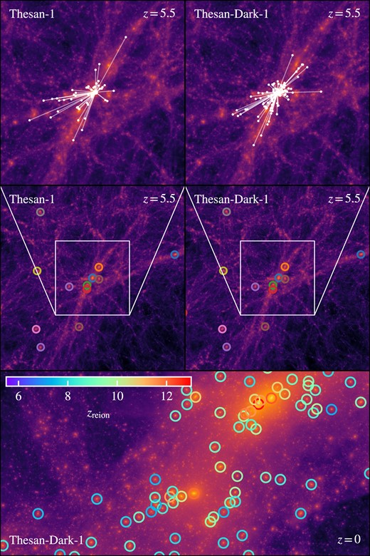
Example of cross-matches between thesan-1 and thesan-dark-1. The central panels show the projected DM density within a 10 cMpc view of the most massive halo at z = 5.5 in thesan-1 (left) and thesan-dark-1 (right). Matches between all subhaloes with mass MH > 1011 M⊙ within this view are shown as circles colour-matched between the two simulation volumes. To highlight potential pitfalls with the matching algorithm, the top two panels show a zoomed-in view of both simulations, with white lines showing all subhaloes that are cross-matched from the other volume to the most massive, central, subhalo. The bottom panel shows the same region, at z = 0 in thesan-dark-1, utilizing cross-links and merger trees to provide reionization timings for all DM subhaloes with MH > 1011 M⊙.
In the top two panels of Fig. 5, we show a case where the output from the cross match files is suboptimal. Each white point and line shows a case in the sibling simulation that is matched to the central substructure, around 50 in both cases. These are subhaloes that have exchanged significant material with the central or are very low mass (and hence close to the resolution limit) and are misidentified in the alternate case as being entirely part of the central subhalo.
The bottom panel of Fig. 5 shows how the cross match catalogues can be used to provide accurate reionization timings for z = 0 bound substructures in thesan-dark-1. Objects have their reionization timing calculated within thesan-1, and are matched to thesan-dark-1. They are then followed to z = 0 using the merger trees (see Section 3.5), allowing us to see the diversity of reionization timings within this highly clustered field.
3.9 Ly α catalogues
File name: Lya_NNN.hdf5
Availability: all RMHD runs
For all snapshots, we produce Ly α catalogues containing additional information for each halo and subhalo, saved in a single HDF5 file. These files mirror the order in the group files; i.e. the additional information relative to the subhalo with global index j is found in each data set of Lya_NNN.hdf5 at position j. In particular, these catalogues provide data on continuum luminosities at 1216, 1500, and 2500 Å, the individual ionizing luminosity contributions of stars, AGNs, collisional excitation emission, and recombination, as well as the Ly α-weighted central position, velocity, and velocity dispersion of the halo. Additionally, we include global Ly α properties as HDF5 attributes of the data sets. The latter are also computed for the ‘fuzzy’ component (i.e. unbound particles) within and between haloes (named ‘inner’ and ‘outer’ following the definition given in Section 3.1), and the entire simulation box (‘total’).
3.10 Lines of sight
File name: rays_NNN.hdf5|$\rm {(for~\tt {N}}\ge 54$|)
Availability: all RMHD runs except the thesan-hr series
We extract gas quantities extracted along a set of random lines of sight (LOS) in the simulation box. The LOS have random origin and direction, have length LLOS = 100 cMpc and employ periodic boundary conditions when necessary. They are extracted using the colt code (most recently described in Smith et al. 2022b), which uses the native Voronoi tessellation of the simulation, therefore retaining the full spatial information available. For this reason, each LOS is composed of a set of segments of different length, corresponding to the intersection between the ray and one Voronoi cell. Notice that each ray has a different number of segments, determined by the native Voronoi structure. For each segment, a number of gas properties are extracted from the Voronoi cell and saved.
We provide 150 LOS for each snapshot from the 54th onward, corresponding to z ≤ 7. Within each LOS file, the properties extracted along the LOS are saved in a number of groups, each one containing a data set for each ray (named simply with a progressive number, starting from 0). This means that, e.g., the density along the third ray is stored in the data set Density/2. In the future we will augment the LOS data with additional relevant catalogues, e.g. lightcones for cosmological integration.
3.11 Filament catalogues
File name: filaments_Fixed{Mass,Number}Tracers_NNN.hdf5
Availability: all RMHD runs except the thesan-hr series
We generate catalogues of cosmic filaments for all simulations within the thesan suite. Filaments are identified in post-processing using the code DisPerSE (Sousbie 2011; Sousbie, Pichon & Kawahara 2011). DisPerSE employs the Discrete Morse theory to identify cosmic filaments from the topology of the density field. In particular, filaments are defined by a set of segments connecting local maxima (‘peaks’) to saddle points, effectively tracing the ridges of the density field. This identification process is governed by the so-called persistence ratio (σ), a metric that quantifies the structural robustness relative to Poisson noise. As a final step, bifurcating filaments (i.e. those that connect a single critical point to multiple saddle points) are split by introducing bifurcation points to avoid double-counting of their shared part.
We have chosen to build the filament catalogues from galaxies, used as tracers of the underlying density field, to closely track the approach commonly adopted in observational studies. From this discrete set of tracers, DisPerSE reconstructs a continuous density field using the Delaunay Tessellation Field Estimator (Schaap & van de Weygaert 2000), optionally including a smoothing procedure based on the moving average over all connected vertices of the tessellation. We provide catalogues following two different tracer selection techniques:
Fixed stellar mass threshold: We use galaxies with stellar mass |$M_\mathrm{star} \ge 10^{7.5} \, {\rm M_\odot }$|, independently of the redshift considered. This results in a decreasing number of tracers with increasing redshift, as is the case in observations. The mass threshold was chosen to approximately match the smallest galaxies routinely observed by JWST (e.g. Santini et al. 2023). In this case, we smooth the inferred density field prior to filament identification and apply a fixed persistence threshold of σ = 3 for all the extractions at different redshift.
Fixed number of tracers: The previous tracer selection method results in structures characteristics of different scales being identified at each redshift, since tracers are increasingly biased with growing redshift. To counteract this effect, we follow the approach proposed by Galárraga-Espinosa et al. (2024). Briefly, tracer selection (resulting in Ntracers tracers) and parameter optimization are performed at the lowest available redshift (z = 5.5). At all other redshifts, we employ the same parameters and apply DisPerSE to an equal number of tracers, selected as the Ntracers galaxies with highest stellar mass. The parameters explored are: the minimum mass threshold for tracers, the smoothing of the reconstructed density field, and the persistence threshold employed. Their optimization was performed by simultaneously maximizing: (i) the number of filament extrema within three virial radii of large haloes (‘peaks in FoF’ in Fig. 6), and (ii) the number of large haloes hosting filament extrema (‘FoF hosting peaks’ in Fig. 6). The first number measures the ‘purity’ of the catalogue, i.e. how many spurious noise-induced filaments are identified, since these are not expected to preferentially lie close to density peaks, unlike real ones. The second measures ‘completeness’ by estimating how many of the largest simulated objects are connected by cosmic filaments, as expected from structure formation theory. In both cases, we defined as large haloes those with |$M_\mathrm{star} \ge 10^{11.5} \, {\rm M_\odot }$|. We illustrate the results of this search in Fig. 6, where the fractions of ‘FoF hosting peaks’ (solid lines) and ‘peaks in FoF’ (dashed lines) are shown as a function of the explored parameter combinations. Coloured curves show the variation as a function of the chosen persistence threshold, while the red circle indicates the chosen parameter combination. We note that the parameter combination (7.5, N, 1.0) seems to be an even better choice (it shows a significantly higher fraction of ‘peaks in FoF’ and similar ‘FoF hosting peaks’). We however decided against its use because the low persistence value produces a large number of spurious filaments, as we confirmed by investigating the filament length distribution, which showed an excess of very short filaments.
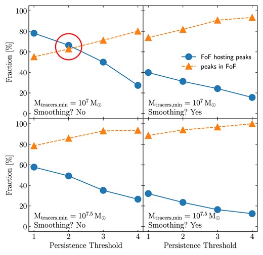
Summary of the calibration performed for the filament catalogues using a fixed number of tracers. The fraction of large haloes (|$M_\mathrm{star} \ge 10^{11.5} \, {\rm M_\odot }$|) hosting filament extrema (‘FoF hosting peaks’, solid lines) and the fraction of filament extrema within large haloes (‘peaks in FoF’, dashed lines) are shown as a function of DisPerSE parameter combinations, namely the minimum tracer stellar mass (|$10^7\, {\rm M_\odot }$| and |$10^{7.5}\, {\rm M_\odot }$| in the top and bottom panels, respectively), the smoothing of the reconstructed density field (applied in the right-side panels and not in the left-side ones), and the persistence threshold employed (varying along the horizontal axis within each panel). The red circle indicates the chosen parameter combination.
The outputs from DisPerSE are re-arranged from the original format7 into an HDF5 file for ease of use, with a structure described on the thesan website.
3.12 Escape fraction catalogues
File name: ion_NNN.hdf5
Availability: all RMHD runs
For all snapshots, we compute the subhalo ionizing escape fraction (i.e. the fraction of ionizing photons that successfully escape the subhalo into the IGM) for each subhalo containing at least one stellar particle and four gas cells within its virial radius. These quantities are provided in catalogues directly mirroring the subhalo catalogues (i.e. the quantities computed for the subhalo with global index j are found in each data set of at position j), contained in a single HDF5 file for each redshift. The actual calculation is fully described in section 2 of Yeh et al. (2023), and briefly summarized in the following.
In practice, the escape fraction is defined as the ratio between the number of ionizing photons that escape the virial radius of the halo and the number of ionizing photons intrinsically emitted from all sources within the same volume. The latter includes the stellar escape fraction assumed in the simulations; i.e. the fraction of photons escaping the unresolved structures around the stellar particle (see column 8 of Table 1). We consider a photon escaped from the halo once it crosses the radius at which the average density reaches 200 times the density of the universe. To ensure consistency, we re-compute all halo properties (mass, SFR, etc.) using this definition of its boundary and provide their values in the catalogues. The intrinsic ionizing photon production rate for each star is computed employing the Binary Population and Spectral Synthesis models (BPASS version 2.2.1; Eldridge et al. 2017; Stanway & Eldridge 2018) with a Chabrier (2003) IMF and is provided in the Ly α catalogues (Section 3.9). The rate of escape of ionizing photons is computed through passive Monte Carlo radiative transfer calculations performed with the Cosmic Ly α Transfer (colt) code (most recently described in Smith et al. 2022b). Finally, whenever a stellar particle is located outside of the virial radius of any halo, we assume that the total (‘halo’) escape fraction equals its stellar escape fraction.
3.13 Galaxy SED catalogues
File name: SED_NNN.hdf5
Availability: thesan-1 at z = 6, 7, 8, 9, 10
For selected redshifts equal to z = 6, 7, 8, 9, and 10 we post-process well-resolved galaxies in the thesan-1 simulation with the Monte Carlo radiative transfer code skirt (Camps & Baes 2020) to produce synthetic spectral energy distributions (SEDs). All galaxies have their SEDs packed in a single file by redshift. The full post-processing methodology for generating them is outlined in section 2.2 of Kannan et al. (2022b), and summarized in the following.
We take the gas and star distributions directly from the simulation itself, while the intrinsic nebular emission is estimated from Byler et al. (2017), who used photoionization calculations carried out with the cloudy code (Ferland et al. 2017). The radiation emitted by stellar particles is computed using the Flexible Stellar Population Synthesis (FSPS) model (Conroy, Gunn & White 2009; Conroy & Gunn 2010). The radiative transfer calculations are performed by skirt on a Voronoi grid constructed from positions of the gas cells in the galaxy (mirroring the structure and geometry of the AREPO data as closely as possible) and cover the wavelength range |$[0.05, 200] \, \mu$|m, discretized into 657 (unequal) bins. Following the considerations presented in section 3.2.3 of Kannan et al. (2022a) we employ a redshift-dependent dust-to-metal ratio instead of the simulated dust distribution. Finally, we assume thermal equilibrium between the dust and the local radiation field as well as a Draine & Li (2007) dust mixture of amorphous silicate and graphitic grains, including polycyclic aromatic hydrocarbons.
Only sufficiently well-resolved, star-forming galaxies are considered to ensure that the produced SEDs are reasonably converged. In particular, an SED is computed for a galaxy if: (i) the stellar mass within twice the stellar half-mass radius is greater than 50 times the baryonic mass resolution of the simulation, and (ii) it contains at least one stellar particle younger than 5 Myr (at the resolution of the simulation this roughly translates to haloes with a minimum SFR of just below |$0.1 \, {\rm M_\odot }$| yr−1).
3.14 ICs
We release the ICs used for all the thesan runs. For the original thesan runs, all ICs correspond to the same (95.5 cMpc)3 volume of the Universe at z = 49, sampled at two different resolutions (corresponding to thesan-1 and thesan-2, respectively). For the thesan-hr series, the ICs correspond to the same (but different from the original thesan) (5.9 cMpc)3 volume of the Universe at z = 49, sampled assuming different models for the dark sector, plus a set of ICs of the same volume at 8 times higher mass resolution (corresponding to the thesan-hr-res8x run) and a set covering a larger (11.8 cMpc)3 box (for the thesan-hr-large) run. All ICs are generated (and provided) as DM-only files. Baryons were included by splitting particles (according to the baryon-to-DM-density ratio) at the startup of the simulation. All the ICs were generated using the N-GenIC version contained in the GADGET-4 code (Springel et al. 2021), using second-order Lagrangian perturbation theory and fixing the amplitude of each density perturbation mode to the power spectrum expectation value (fixed approach from Angulo & Pontzen 2016). This ensures that the ICs generated are fully representative of the average Universe on all scales sampled.
4 USAGE CONSIDERATIONS
4.1 Data retrieval
We rely on the globus8 file transfer service to make the thesan data public. This infrastructure provides a solid, flexible, and efficient system to transfer data, alongside with fine-grained customization options. It features a browser-based interface as well as command-line and python access options, automatic verification of data integrity and autonomous handling of connection interruptions. The globus workflow involves endpoints, i.e. machines where the globus application has been installed. Users can initialize data transfer between two endpoints and let globus handle the execution. Alternatively, it is possible to download the data via simple direct download at the price of losing the features listed above. The thesan data are stored in a collection named ‘Thesan’, stored at the endpoint ‘MPCDF DataHub Server’. A direct link to the collection can be found at https://www.thesan-project.com/data.html, alongside detailed documentation and a short globus tutorial. The organization of the released data into directories is shown in Fig. 7. Please notice the citation policy on the website, which ensure that the contributions of all individuals involved in the development of the thesan simulation suite are properly acknowledge.

Organization of the public thesan data directory with subsection references. For the sake of brevity, we have omitted from the figure some of the less important files, as well as the content of the postprocessing sub-directories, which have been thoroughly described in Section 3 or the online documentation.
4.2 Physical considerations
thesan builds upon the successful IllustrisTNG galaxy formation model, inheriting both its strengths and limitations. Notably the inclusion of self-consistent RT makes thesan particularly well suited for studying the z ≳ 5 Universe. In the following, we outline and briefly comment on several aspects of thesan that warrant cautious interpretation.
4.2.1 Numerical convergence
Numerical convergence is a crucial factor in assessing the reliability of simulation outcomes. Different physical quantities often reach convergence at different resolution levels, and careful comparisons are required to understand the quantitative accuracy of measurements derived from the simulations.
For thesan it is critical to consider the SFRD and its convergence, due to the direct link between the SFRD and ionizing photon budget, especially given our fixed choice of fesc for stars. In Fig. 8 we show the SFRD for both thesan-1 and thesan-2, and highlight that thesan-1 exhibits a higher SFR at high redshifts – a factor of ≈1 dex at z ≳ 13, decreasing to a factor of 1.5 at z ≲ 8. With a mass resolution eight times higher than that of thesan-2, along with correspondingly smaller softening scales, thesan-1 is capable of resolving higher gas densities and hence earlier star formation.
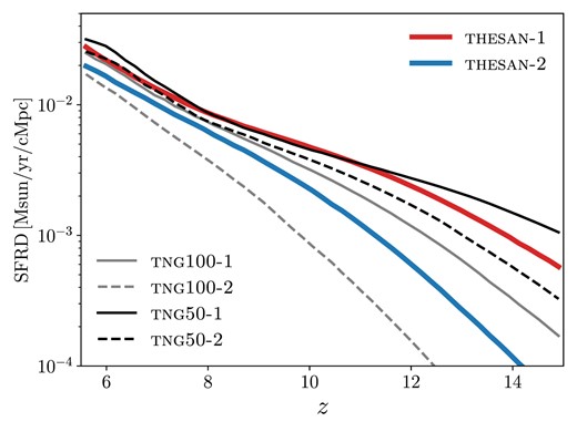
Comparison of the SFRD in the thesan-1, thesan-2, IllustrisTNG-100-1, IllustrisTNG-100-2, IllustrisTNG-50-1, and IllustrisTNG-50-2 simulations. As discussed in Borrow et al. (2023) the inclusion of radiation in thesan leads to a suppression of star formation relative to models using a spatially uniform UV background at z ≳ 10.
To show that we have almost reached numerical convergence of the SFRD in thesan-1, we can employ the already existing IllustrisTNG-100 and IllustrisTNG-50 simulations, which have box volumes with side lengths of 106.5 and 51.7 cMpc, respectively. Fig. 8 shows four comparison simulations in these two box volumes with the following mass resolutions: TNG100-1 (mgas = 1.4 × 10⁶ M⊙), TNG100-2 (mgas = 1.1 × 10⁷ M⊙), TNG50-1 (mgas = 8.4 × 10⁴ M⊙), and TNG50-2 (mgas = 6.8 × 10⁵ M⊙). thesan-1 has a resolution close to TNG50-2, and thesan-2 has a resolution between TNG100-1 and TNG100-2. There are only relatively minor differences between the SFRD in TNG50-1, TNG50-2, and thesan-1, indicating that we are close to a numerically converged model. Specifically, the SFRD differences above z ≳ 14 are within a factor of ≈2, with the onset of star formation only occurring around z ≈ 16. For thesan-2, however, there are significant differences between the two TNG100 resolution levels, with thesan-2 lying in between, indicating that numerical convergence has not yet been attained for this simulation.
A second key numerical parameter worth discussing here in more details is the minimum simulation volume required to provide converged predictions of reionization properties, which remains unclear. In particular, Iliev et al. (2014) found that volumes of approximately 100 |$h^{-1}\, {\rm Mpc}$| are sufficient for good convergence of most simulated IGM properties, with the exception of the 21-cm signal requiring volumes of at least 250 |$h^{-1}\, {\rm Mpc}$|. However, these simulations do not account for Lyman-limit system, resulting in a likely over-estimation of the necessary volumes (see also the discussion in section 6.4 of Gnedin & Madau 2022). Finally, Gnedin & Kaurov (2014) showed that in the CROC simulations (in many ways similar to thesan in terms of physical richness, resolution and ability to reproduce observed IGM properties) boxes as small as 20 |$h^{-1}\, {\rm Mpc}$| are sufficient for the convergence of the ionized bubble size distribution at z > 7. Concerning thesan, we do not have access to runs with equal resolution in different box sizes, but fig. 2 of Neyer et al. (2023) shows no signs of truncation of the bubble size distribution until towards the very end of the reionization history. Moreover, we have confirmed that the simulated reionization history, IGM temperature, CMB optical depth, and bubble size distribution are practically unchanged when the entire simulation box is divided into eight independent sub-boxes (see fig. 3 of Paper ii for a visualisation of the first three). While not exactly equivalent to a volume convergence study, these facts give us confidence that that reionization properties are likely converged with respect to the simulated volume in our runs.
4.2.2 Reionization history
As described in Section 2, the escape fraction of ionizing photons from stars was tuned to obtain a model within which reionization occurs late, with this calibration performed at the thesan-2 resolution. Results from Paper ii suggest that reionization in thesan-1 may still end slightly too early. This discrepancy is attributed to a resolution-induced factor of ∼3 excess in the early SFRD, as seen in Fig. 8. Given that fesc was not re-calibrated between different resolution levels, thesan-1 consequently has a higher budget of ionizing photons.
4.2.3 Cosmic dust
We advise the reader to exercise caution regarding the cosmic dust content of massive galaxies within the thesan simulation suite. Preliminary analysis suggests that the dust buildup may be too low compared to observational data. The main evidence is the insufficient attenuation at the bright end of the UV luminosity function when the simulated dust content is used (see fig. 11 of Paper i). While this discrepancy is not entirely surprising, since we made the deliberate choice to not tweak any parameter in the model and adopt the original calibration by McKinnon et al. (2016, 2017), which is based on Milky Way data. However, this evidence is not conclusive, since the issue may lie in the attenuation law used for dust. We are currently investigating this topic further.
4.2.4 Unresolved interstellar medium
thesan employs the two-phase interstellar medium (ISM) model proposed by Springel & Hernquist (2003). By design, this model precludes any attempt to self-consistently resolve the multiphase ISM. This approach is necessary to achieve the large volume of the thesan runs, which prevents us from reaching the resolution required for more self-consistent treatments of the ISM. Consequently, the cold dense and molecular phases of the ISM, giant molecular clouds, and individual stellar birth clouds are not explicitly resolved. The modelling of observables predominantly arising from these unresolved phases should be undertaken with care.
4.3 Data analysis
The majority of the data released, including snapshots, group catalogues, merger trees, and offset files, have structures similar to that of the IllustrisTNG data sets. This facilitates the straightforward adaptation of existing tools for use with thesan data. To further streamline data utilization associated with this paper, we have updated the widely used python module illustris_python (along with its twin modules for the julia, matlab, and idl programming languages) to work with thesan data and to support the loading of our Cartesian outputs.9
5 COMPARISON WITH JWST RESULTS
The successful launch and deployment of the JWST has quickly transformed the study of the z ≳ 5 Universe. Within just a year, it has already started to reshape our understanding of primeval galaxy formation and reionization. Simultaneously, it has significantly extended our ability to test the current models of galaxy formation in the young Universe. This is of crucial importance as these models were typically devised and calibrated when such observations were not available, and therefore provide genuine predictions about the properties of the galaxy candidates recently uncovered. In fact, many inherently different galaxy formation models have reached comparable success in reproducing the observed galaxy population, both at low (Khandai et al. 2015; Schaye et al. 2015; Dolag et al. 2016; Tremmel et al. 2017; Marinacci et al. 2018; Naiman et al. 2018; Nelson et al. 2018; Pillepich et al. 2018b; Springel et al. 2018; Dubois et al. 2021) and high redshift (Gnedin 2014; Pawlik et al. 2017; Rosdahl et al. 2018; Trebitsch et al. 2021; Garaldi et al. 2022; Kannan et al. 2022a; Smith et al. 2022a). Comparing their predictions to new data in a redshift range relatively uncharted so far is therefore a key test of these models, one that could differentiate these models, and thus a prime way to advance our knowledge of the onset of galaxy formation.
In this section we compare the predictions of thesan with a selection of results from the JWST to serve multiple objectives. First, this exercise tests the reliability of the thesan simulation suite, pinpointing areas for refinement. Secondly, contrasting these results with similar analyses performed on simulations employing different physical and numerical prescriptions highlights the strengths and weaknesses of each model. This, in turn, improves our understanding of primeval galaxy formation and eventually guides the development of the next generation of numerical simulations. Thirdly, these comparisons serve as examples of how the publicly released thesan data can be leveraged for the interpretation of observations. To facilitate the latter, we specify at the beginning of each subsection the data products employed for the ensuing analyses and discussions.
5.1 Galaxy spectra and images
Data product used: snapshots, offset files
Among the first and most surprising results from the JWST is the identification of a significant number of galaxy candidates at z ≳ 8 with large stellar masses (e.g. Castellano et al. 2022; Labbe et al. 2023; Naidu et al. 2022; Tacchella et al. 2022; Yan et al. 2022; Atek et al. 2023b; Austin et al. 2023; Curtis-Lake et al. 2023; Finkelstein et al. 2023; Morishita & Stiavelli 2023). While a thorough comparison with comparison with each one of these (and many more) works is beyond the scope of this paper, we provide a methodological example using individual galaxies extracted from the thesan-1 simulation. Utilizing the skirt code (Camps & Baes 2020), we simulate the propagation of radiation until it escapes the galaxy (for a detailed description of the SED production, see Kannan et al. 2022b). We additionally account for attenuation from the intervening IGM following Madau (1995). Finally, we coarsen the images to match the NIRCam resolution of 0.07 arcsec, corresponding to approximately 0.3 kpc at z = 10, and add Gaussian random noise assuming a signal-to-noise of 30 for the image, comparable to the one achieved for z ≳ 8 galaxies in the field of SMACS J0723.3-7327 (Pontoppidan et al. 2022). The results of this procedure are presented in Fig. 9 for a selection of the brightest thesan-1 galaxies at z = 10. The mock images shown in the top two rows correspond to the view of the galaxies in the f277w filter of the JWST, while the bottom row shows the synthetic observation of one galaxy across a number of JWST filters (reported in the top left corner of each plot). All panels have a linear size of 10 kpc (33 pixels). Even from such a small sample it is possible to appreciate the diverse variety of galactic morphologies, ranging from isolated galaxies to active mergers. In particular, we also observe aligned structures, reminiscent of the cosmic filaments observed by Wang et al. (2023). We have not yet investigated whether these are physically associated structures or merely an effect of galaxy selection and alignment. The released thesan data are well-suited for such investigations.
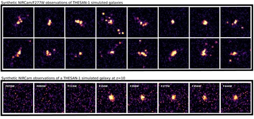
JWST mock images of bright galaxies (top two rows) found in thesan-1 at z = 10, using the F277W filter and a noise level comparable to the early science release data in the field of SMACS J0723.3-7327. The bottom row shows how the largest galaxy in thesan-1 at z = 10 would appear in a series of JWST filters (reported in the top left corner of each plot).
Encouraged by this qualitative agreement with recent observations, we proceed to a more quantitative exploration in the following subsections.
5.2 The galaxy main sequence at z > 6
Data product used: group catalogues, SEDs
The majority of low-redshift galaxies adhere to a well-established relationship between their total stellar mass (Mstar) and their SFR, commonly referred to as the galaxy main sequence (GMS). Whether such a relation holds at high redshifts is currently being investigated by the JWST (e.g. Finkelstein et al. 2022; Roberts-Borsani et al. 2022; Stefanon et al. 2022; Tacchella et al. 2022; Chen et al. 2023; Leethochawalit et al. 2023). In Fig. 10, we present this relation for thesan-1 at integer redshifts between 6 and 10, depicted as solid lines. For the sake of clarity, the central 68 per cent of the data is shown only for z = 8 as a shaded region, although the distribution is similar for the other redshifts. The figure also reports a number of recent observations about candidate galaxies identified via the JWST. We find an overall good agreement between these results and our model predictions, with two notable exceptions: (i) For galaxies with stellar masses |$M_\mathrm{star} \lesssim 10^{8} \, {\rm M_\odot }$|, Stefanon et al. (2022) and Chen et al. (2023) report significantly higher SFRs than those found in thesan-1. (ii) For galaxies with stellar masses |$M_\mathrm{star} \gtrsim 10^{9} \, {\rm M_\odot }$|, the data appear to bifurcate into two distinct sequences, one in excellent agreement with thesan-1 and a second with galaxies exhibiting SFR 50–100 times lower. The frequency and origins of these quenched galaxies remain topics of ongoing debate, especially as only the advent of JWST uncovered such population of galaxies. Below we discuss a recent extreme example of such a quenched galaxy, as reported by Looser et al. (2023).
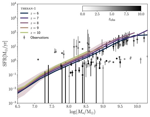
Galaxy main sequence at z = 6, 7, 8, 9, and 10 in thesan-1 (coloured curves), compared to the values from observations by Finkelstein et al. (2022), Stefanon et al. (2022), Tacchella et al. (2022), Roberts-Borsani et al. (2022a), Asada et al. (2023), Chen et al. (2023), Fujimoto et al. (2023), Leethochawalit et al. (2023), Long et al. (2023), Pérez-González et al. (2023), Sun et al. (2023), Treu et al. (2023), Arrabal Haro et al. (2023a), Atek et al. (2023a), Jung et al. (2023), and Arrabal Haro et al. (2023b). All observations are colour-coded by their redshift, as reported in the top colour bar. The shaded region shows the central 68 per cent of data, only for z = 8 for visual clarity.
thesan predicts a modest decrease of the normalization of the GMS over cosmic time, almost uniformly across the mass range covered by the simulation. Utilizing the different runs within the thesan suite, we can predict the influence of different physical models on the GMS. This is shown in Fig. 11, where we present the GMS at z = 8 for the different thesan runs. Over the mass range covered here, there is no apparent difference in the GMS between the different runs. The only minor effect is a small suppression of star formation at the lowest stellar masses in the thesan-2 runs, dictated by the limited resolution within the smallest haloes. However, as demonstrated in Shen et al. (2024) using the thesan-hr simulation set, different DM models do have an impact on galaxies at lower mass scales.
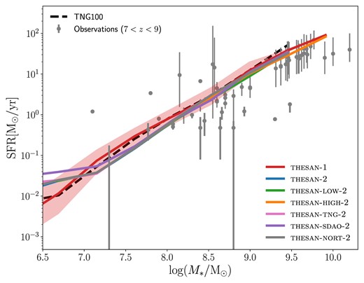
Same as Fig. 10 but showing only the relation at z = 8 for the different thesan runs as well as for TNG100 and for observations at 7 ≤ z ≤ 9. In this case, the shaded region showing the central 68 per cent of data is shown only for z = 8 (again for visual clarity).
5.2.1 Quenched galaxies in thesan
Recently, Looser et al. (2023) reported the discovery of a galaxy with a stellar mass of |$M_\mathrm{star} \approx 10^{8.7} \, {\rm M_\odot }$| and an exceptionally low SFR (log (SFR[M⊙ yr−1]) ≈ −2.5). The SED modelling of this galaxy indicates that this object was quenched between 10 and 38 Myr before it was observed, after a starburst lasting ∼50 Myr. To investigate the presence of similar objects in thesan and explore the conditions under which they might occur, we recompute for each galaxy its SFR over a time window of Δt = 38 Myr.
The thesan-1 simulation does not contain any galaxies exactly matching all of these quenching properties, but there is an analogous population of reasonably similar objects with log (SFR) ∼ −2. In fact, there are at least two different reasons why thesan-1 is not expected to exactly match such observations, namely: (i) the limited volume restricts the range of galaxy properties that can be represented and (ii) the finite baryonic resolution limits the minimum SFR that can be resolved. In fact, the lowest SFR over a time window Δt that can be obtained is simply the minimum stellar mass that can be resolved divided by Δt itself. Given the gas mass resolution of thesan-1 (see Table 1), and the fact that arepo is designed to keep gas masses within a factor of 2 of the target resolution mgas, we can estimate the smallest SFR detectable in thesan-1 as
where we have used Δt = 38 Myr. Therefore, thesan-1 is not able to detect an SFR as low as the one reported by Looser et al. (2023). In addition, we have disregarded any potential obscuration effects from cosmic dust which could further conceal the light from newborn stars. Notice that this calculation does not apply to the SFR reported e.g. in Figs 10 and 11, since in these cases we report the instantaneous SFR, computed internally by the simulation at run time from the gas bulk properties only (following Springel & Hernquist 2003), and is therefore not affected by mass resolution.
In Shen et al. (2024), we have expanded on this analysis using a more flexible definition of quenching. This resulted in the identification and characterization of high-mass quenched objects.
5.3 Obscured star formation
Data product used: group catalogues, SEDs.
The phenomenon of obscured star formation is a crucial consideration in the study of galaxy evolution. Newborn stars typically emit intense UV radiation, rendering the UV luminosity a useful proxy for the star-formation activity of a galaxy. However, when the galaxy hosts a substantial dust content, the latter can absorb and reprocess a significant fraction of UV light into the infrared (IR), effectively hiding it. This is often referred to as obscured star formation, and can be revealed by detecting the IR light emitted by cosmic dust (Madau & Dickinson 2014). Recent observational efforts have started to constrain the fraction of obscured star formation in the Universe across cosmic time, yielding precious information on both the star-formation activity and the dust content of ancient galaxies.
Thanks to the rich physics contained in the thesan simulations, it is possible to estimate the amount of obscured and unobscured star formation for each galaxy, albeit with the limitations described in Section 4.2. In order to properly compare our results to observations, we follow Shen et al. (2022) and calculate for each galaxy obscured and unobscured SFRs from their synthetic SED (see Section 3.13). We convert the total luminosity in the UV (1450–1550 Å) and IR (8–1000 μm) bands directly into SFRs using the conversion rates provided by Madau & Dickinson (2014).10 In Fig. 12, we show the ratio between the IR- and UV-inferred SFRs at z = 6 for star-forming galaxies in thesan-1, plotted as a function of their stellar mass. Each pixel of this two-dimensional map is colour-coded according to the average gas metallicity of the galaxies it represents, reflecting their cosmic dust content. As expected, more massive galaxies are dominated by obscured star formation, thanks to the large amount of dust that they host. In contrast, low-mass galaxies are well characterized by UV-inferred star formation. The top panel of the figure shows the average fraction of obscured star formation in galaxies as a function of their stellar mass.
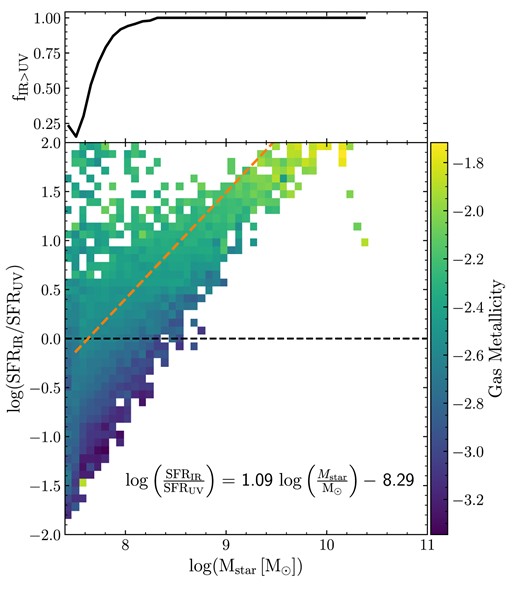
Top: Fraction of obscured star formation in simulated galaxies as a function of their stellar mass in thesan-1. Bottom: Distribution of the ratio between the IR- and UV-inferred SFR at z = 6 for star-forming galaxies in thesan-1 and their stellar mass, colour-coded by the average gas metallicity of the galaxies in each pixel, as a proxy for their dust content. Obscured star formation dominates in more massive galaxies, where the largest reservoirs of cosmic dust (reflected in their gas metallicity) are found, while it is subdominant in smaller objects. At fixed stellar mass, the relevance of obscured star formation correlates with the gas metal content. The orange dashed line shows the best-fit linear relation, also reported in the bottom right.
As a simple example of how this knowledge can help decipher observations, we provide the best-fit linear relation between the IR-to-UV SFR ratio and log (Mstar/M⊙) for the thesan-1 galaxies at z = 6. This can provide useful information to gauge the amount of star formation revealed or obscured in a given observation. We caution that this approach is simplistic and is primarily intended as an example of the science enabled by thesan. However, the IR-to-UV SFR ratio depends on the galaxy gas metallicity, and potentially more properties, that should be taken into account.
5.4 The mass–metallicity relation at z > 6
Data product used: group catalogues.
The advent of JWST has significantly advanced studies of the composition of galaxies deep in the reionization epoch beyond what can be inferred from their luminosities. In particular, the stellar mass–gas metallicity relation (MZR) has become an active area of interest. Fig. 13 shows the MZR for thesan-1 at five different redshifts, while the impact of different numerical and modelling assumptions is then shown (at z = 8) in Fig. 14. In the latter, we also report the results computed from the Illustris-TNG 100 simulation. In both plots, the gas-phase O/H abundance ratio reported in observations has been converted to total gas-phase metallicities assuming a hydrogen mass fractions of 74 per cent and that oxygen makes up 35 per cent of the total metal mass. In summary, thesan-1 shows no redshift evolution in the MZR, including its scatter (which, for the sake of clarity, we show only for z = 8). At all redshifts investigated, thesan appears to predict slightly too many metals at a fixed stellar mass compared to the bulk of available observations. This is in line with the likely underestimation of the cosmic dust content of galaxies (see Paper i), which leaves too many metals in the dust phase, thereby affecting the MZR. This particular aspect warrants further investigation, which we are carrying out.
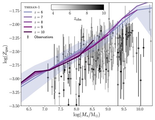
Mass–metallicity relation at z = 6, 7, 8, 9, and 10 in thesan-1 (coloured curves), compared to observations over the redshift range z ≳ 4.8 from Langeroodi et al. (2023), Schaerer et al. (2022), Roberts-Borsani et al. (2022), Boyett et al. (2023), Curti et al. (2023), Fujimoto et al. (2023), Nakajima et al. (2023), Trump et al. (2023), Williams et al. (2023), and Bunker et al. (2023), colour-coded by their redshift as indicated in the colourbar at the top.
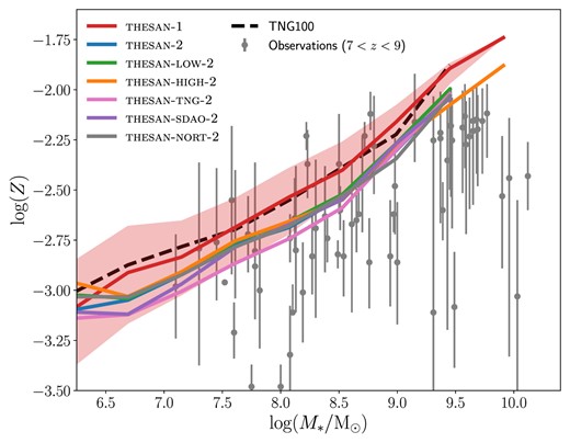
Same as Fig. 13 but showing only the relation at z = 8 for the different thesan runs, as well as for TNG100 and for observations in the redshift range 7 ≤ z ≤ 9.
Finally, explored variations in the physical models in the thesan simulations seem to leave little imprint on the MZR, as seen in Fig. 14. In fact, it appears that the main difference in the runs is due to the different resolutions employed, with thesan-1 showing higher metallicities at any given stellar mass compared to the other runs. This is consistent with the slightly earlier onset and higher amount of star formation due to its higher resolution. However, Borrow et al. (2023) used the thesan-hr runs to show that the radiation modelling has an impact on the metal enrichment of the lowest-mass systems. Similarly, Shen et al. (2024) used the same simulations to show that some beyond-CDM models also suppress the metal production in low-mass systems. Thus, while resolution is a significant factor, other physical and numerical considerations can also play a role.
5.5 UV slopes
Data product used: merger trees, Ly α catalogues, SEDs
The power-law index β of the rest-frame galaxy UV continuum, often called UV slope, is influenced by the stellar ages and the metal content within the galaxy itself. As such, it is often used as an indicator of very young, extremely metal poor, dust free galaxies (e.g. Cullen et al. 2023), which should approach the threshold value β ≈ −3 (Schaerer 2002). Additionally, the nebular emission from free-bound and two-photon processes can easily redden the slope, requiring a large ionizing escape fraction to attain β ≈ −3, suppressing the contribution of nebular continuum. Therefore, a blue β value is used to identify LyC leaker candidates and agents of reionization. Until the advent of the JWST, the bluest galaxies known showed β ≈ −2.5 (e.g. Calzetti, Kinney & Storchi-Bergmann 1994; McLure et al. 2018). Observational biases can also create artificially blue slopes (e.g. Dunlop et al. 2012; Rogers, McLure & Dunlop 2013). Interestingly, the first galaxies robustly observed by the JWST have β values that are, on average, no bluer than in the local Universe (e.g. Cullen et al. 2023).
In Fig. 15, we show the β-slopes versus galaxy UV magnitude MUV plane across five different redshift windows. The background two-dimensional histogram shows the predictions from thesan-1, generated using synthetic SEDs (see Section 3.13 and Kannan et al. 2022b, for details on how they were obtained). The colour is logarithmically scaled from light to dark with the number of galaxies in the histogram bin. Overplotted with thin coloured symbols is a collection of recent JWST observations (Endsley et al. 2023; Austin et al. 2023; Cullen et al. 2023; Curtis-Lake et al. 2023; Franco et al. 2023; Atek et al. 2023b), Tacchella et al. (2022), Topping et al. (2022), and Whitler et al. (2023a, b). Additionally, to highlight the evolutionary paths of galaxies through this plane, we show with different thick symbols where five randomly selected galaxies lie on this plane at each redshift. The symbol colours encode simulated properties of the galaxies, namely its escape fraction (inner colour, with darker red pointing to a higher escape fraction) and dust content (outer colour, with darker blue indicating more dust). Finally, the dashed grey horizontal line marks the theoretical threshold value of β = −3.
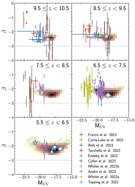
Distribution of UV magnitudes MUV and slopes β for candidate galaxies at z = 6, 7, 8, 9, 10 in thesan-1 (background shading) compared to recent observations from Atek et al. (2023b), Austin et al. (2023), Cullen et al. (2023), Curtis-Lake et al. (2023), Endsley et al. (2023), Franco et al. (2023), Tacchella et al. (2022), Topping et al. (2022), and Whitler et al. (2023a, b). We show five randomly selected simulated galaxies with different symbols, to highlight how they evolve in the diagram. The inner colour of the symbol contours encodes the galaxy escape fraction (with darker red pointing to a higher escape fraction), while the outer colour reflects the galaxy dust content (with darker blue indicating more dust). Finally, we indicate the threshold value β = −3 with a dashed grey horizontal line.
The thesan galaxies lie in a U-shaped distribution (but see below). Objects with MUV ≈ −18 tend to have the bluest UV slopes, averaging around β ≈ −2.5. Brighter galaxies have, on average, larger dust masses which pushes β to redder values. Conversely, UV-fainter galaxies typically have older stellar populations, which reduces their UV flux and increases their β slopes. It is important to clarify that this U-shaped pattern does not imply that all UV-faint thesan galaxies have redder slopes with respect to MUV ≈ −18 ones. Rather, this is partially a consequence of the fact that synthetic SED (and therefore UV slopes) have been computed (to this date) only for the largest galaxies in the simulation, because of the relatively large computational time required. Using the Mstar–MUV relation measured at z = 6 by Bhatawdekar et al. (2019), we estimate that such a selection effect is significant for galaxies fainter than MUV ≳ −18.3. Brighter galaxies in thesan generally align well with observed UV slopes, although observations exhibit a larger scatter compared to our simulations. However, it should be noted that most of the observed data points have large errors and are based on photometric measurements. Additionally, thesan-1 covers only a relatively small volume, and is therefore unable to capture rare objects such as very UV-bright galaxies.
5.6 Ionizing photon production efficiency
Data product used: snapshots, offset files, Ly α catalogues, SEDs
A key quantity in our understanding of cosmic reionization as well as high-z galaxy formation is the ionizing photon production efficiency ξion. This is defined as the ratio between the rate of production of photons with energy |$E_\gamma \ge 13.6\, eV$| and the UV luminosity of a galaxy, i.e. |$\xi _\mathrm{ion} = \dot{N}_\mathrm{ion}/M_\mathrm{UV}$|, where |$\dot{N}_\mathrm{ion}$| is the intrinsic rate of ionizing photons production and MUV is the galaxy UV magnitude. Therefore, this value contains information about the stellar population of a galaxy (e.g. age, IMF) and its dust obscuration (through the UV luminosity).
Thanks to the capabilities of the JWST, this quantity can now be routinely measured in z ≳ 5 galaxies. In Fig. 16, we present these measurements (from Bouwens et al. 2016; Endsley & Stark 2022; Saxena et al. 2024; Simmonds et al. 2023; Bunker et al. 2023; Jung et al. 2023) as grey points, together with the predictions from the thesan-1 simulation at integer redshifts. The latter are represented as violin plots, where the shaded areas indicate the distribution of ξion values, and the median is marked by symbols. Specifically, the left half of each violin and the star symbols refer to the intrinsic values of ξion, while the right half of the distribution and the diamonds are computed including dust attenuation. The values of ξion were computed combining the individual stellar particles of a galaxy with the BPASS v2.1 stellar library (the same used within the simulation) to determine the ionizing photons production rate, while the (dust-attenuated) UV luminosity is taken directly from the synthetic SED (see Section 3.13). The simulated values overlap well with the observed ones, but with the caveat that thesan-1 does not contain galaxies with ξion ≳ 25.8 that are however found in observations. This discrepancy might be due to the limited simulated volume, which fails to capture rare objects, or to the assumed stellar population model and IMF.
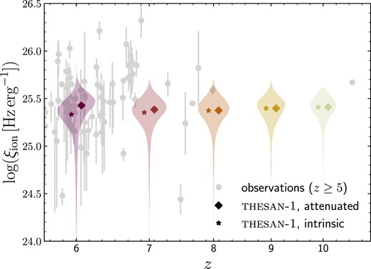
Redshift evolution of the ionizing photon production efficiency ξion in thesan-1. The vertical violin plots show the distribution of values at a given redshift. For each of them, the right half shows the ξion values including dust attenuation, while the left half shows the distribution of intrinsic values. The medians of these distributions are indicated by star and diamond symbols, respectively. The grey points correspond to a collection of observed values (Bouwens et al. 2016; Endsley & Stark 2022; Bunker et al. 2023; Jung et al. 2023; Saxena et al. 2024; Simmonds et al. 2023).
We do not observe any evolution with time in the bulk of the distributions, nor significant dependence on UV magnitude or stellar mass (not shown in the figure). At the same time, the ξion of an individual galaxy varies strongly during its lifetime. Taken together, these results indicate that the population-averaged ionizing photon output does not vary significantly over the interval 6 ≤ z ≤ 10. Instead, the growth of the galaxy population and the increase of the total stellar mass in the Universe is what advances and accelerates reionization towards z ∼ 6. It should be noted, however, that the high-ξion tail of the distribution is cut short at higher redshift. This truncation is due to a combination of poorer statistics (i.e. fewer galaxies) and a general absence of massive, dusty galaxies. The latter, in fact, lowers the observed UV luminosity, increasing ξion at a fixed production rate of ionizing photons. Therefore, the formation of an increasing amount of dust can drive up ξion values at lower redshifts, even if the intrinsic properties of galaxies remain unchanged. This can be appreciated comparing the two sides of the violin plots, which makes apparent that dust obscuration starts to have an impact on the distribution of observed ξion only at z ≲ 7.
6 SUMMARY AND CONCLUSIONS
As part of this paper, we have publicly released the entire set of data and data products generated from the thesan simulation suite, including the raw simulation outputs. These resources are freely accessible to the research community and come with complete documentation. They can be downloaded from the project’s official website: https://thesan-project.com. This release aims to facilitate further research and progress in the interconnected fields of galaxy formation and cosmic reionization.
thesan is a suite of RMHD simulations designed to simultaneously capture the cosmological scales required for reionization modelling and the ∼100 pc resolved physics responsible for galaxy formation in the high-redshift (z ≥ 5) Universe. It incorporates the IllustrisTNG galaxy formation model, self-consistent RT of photons emitted by both stars (including binary systems) and quasars, a sophisticated model for the creation, evolution, and destruction of cosmic dust, and variance-suppressed ICs. The main series of simulations follows a large volume (95.5 cMpc)3 of the Universe under different physical models for the escape of ionizing radiation from galaxies and for the nature of DM. Alongside these, we have also released data from the thesan-hr series, which consists of even higher-resolution simulations in smaller volumes, specifically designed to investigate non-trivial effects of reionization on the properties of lower-mass galaxies.
thesan augments traditional simulation outputs, such as snapshots and group catalogues, with novel high-time-cadence Cartesian outputs and a wide range of post-processing data products. These are thoroughly described in this paper with additional details in the online documentation, and are publicly available as well. In order to ease the usage of thesan by researchers with varying expertise, we have integrated support for thesan data into widely used analysis tools.
The thesan simulations offers robust predictions that align well with recent observations from the JWST concerning galaxies in the first billion years of the Universe, as we have shown in the second part of this manuscript. Specifically, thesan matches key relations such as the galaxy main sequence, the mass–metallicity relation, and the UV slope–stellar mass relation at z ≥ 6. Additionally, the simulations provide forecasts for the fraction of dust-obscured star formation as a function of galaxy mass. Leveraging the physical variations simulated within the thesan project, we show how these important quantities are influenced by the still-uncertain physics at high redshifts.
thesan represents the present state of the art in simulating the first billion years of cosmic history, from IGM to CGM and galactic scales. We have made the entire data of the project fully available to the community in the hope that researchers across the world will contribute to fully exploiting the potential of these simulations. As new data are generated and vetted, they will be added to the thesan repository and accompanied by updated documentation on the project website.
Finally, the thesan project is an ongoing and continually evolving initiative. Broadly speaking, we are currently focusing on three parallel programmes embodying the near-term futures of thesan. First, we aim to increase the simulated volume to both capture rarer objects and reach sufficiently large scales to more effectively interface with 21-cm cosmology, including improved sampling of lower modes of the power spectrum. Secondly, we are entering the production stage of developing zoom-in re-simulations that incorporate a model for the multiphase ISM, the large-scale radiation field of thesan, and extend to significantly lower redshifts than the original thesan volume. Thirdly, we plan to conduct re-simulations of individual sub-volumes within the thesan box, each with different reionization histories and varying environmental overdensities, to rigorously assess the impact of local reionization on a statistically significant population of highly resolved galaxies. In summary, the thesan project invites extensive direct and indirect community collaboration to advance these targeted efforts, thereby promising to transform our understanding of cosmic reionization and early galaxy formation.
ACKNOWLEDGEMENTS
We are grateful to the referee, Nick Gnedin, for his insightful comments, which improved our manuscript. EG acknowledges support from the CANON Foundation Europe through the Canon Fellowship program during part of the work presented in this paper. RK and AS acknowledge support under Institute for Theory and Computation Fellowships at the Center for Astrophysics | Harvard & Smithsonian, and AS for program number HST-HF2-51421.001-A provided by NASA through a grant from the Space Telescope Science Institute, which is operated by the Association of Universities for Research in Astronomy, incorporated, under NASA contract NAS5-26555. MV acknowledges support through NASA ATP grants 16-ATP16-0167, 19-ATP19-0019, 19-ATP19-0020, 19-ATP19-0167, and NSF grants AST-1814053, AST-1814259, AST-1909831, and AST-2007355. The authors gratefully acknowledge the Max Planck Computing and Data Facility (https://www.mpcdf.mpg.de/) for support in hosting data and releasing them to the public, as well as the Gauss Centre for Supercomputing e.V. (www.gauss-centre.eu) for funding this project by providing computing time on the GCS Supercomputer SuperMUC-NG at Leibniz Supercomputing Centre (www.lrz.de). Additional computing resources were provided by the Extreme Science and Engineering Discovery Environment (XSEDE), at Stampede2 through allocation TG-AST200007, by the NASA High-End Computing (HEC) Program through the NASA Advanced Supercomputing (NAS) Division at Ames Research Center, and the Engaging cluster supported by the Massachusetts Institute of Technology. We are thankful to the community developing and maintaining software packages extensively used in our work, namely: matplotlib (Hunter 2007), numpy (Walt, Colbert & Varoquaux 2011), scipy (Jones et al. 2001), cmasher (van der Velden 2020), and corecon (Garaldi 2023).
DATA AVAILABILITY
All data produced within the thesan project are made fully and openly available at https://thesan-project.com, including extensive documentation and usage examples. We invite inquiries and collaboration requests from the community.
Footnotes
The volume required for convergence of reionization properties remains unclear. We discuss this and substantiate our claim in Section 4.2
In principle, despite sharing the same galaxy-formation model, some thesan galaxies might differ from those produced by the original IllustrisTNG model, since we have upgraded from equilibrium to non-equilibrium cooling in thesan. However, we have confirmed that this change does not significantly impact the properties of simulated galaxies with a halo mass of |$M_\mathrm{halo} \gtrsim 10^{9} \, {\rm M_\odot }$| at the latest available redshift (z = 5.5). Smaller galaxies are impacted by the self-consistent treatment of RT, and therefore are expected to differ irrespective of the cooling treatment.
If not otherwise specified, all ionized fraction quoted in the paper are volume weighted, as customary in studies of cosmic reionization.
This organization allows one to easily locate the particles belonging to a given FOF group or subhalo from the knowledge of just the number of particles belonging to each subhalo in the simulation, optimizing the storage by circumventing the need to save the particles identifiers. In order to speed up the particle loading, we have created auxiliary files (namely, the offset files described in Section 3.6 for a halo- or subhalo-based loading, and the hashtables described in Section 3.7 for a position-based loading).
The code used to read and re-arrange the DisPerSE output can be found at https://github.com/EGaraldi/disperse_output_reader.
Using this updated version requires re-downloading and re-installing the packages from:
