


ABSTRACT
We use 3D computer modelling to investigate the time-scales and radiative output from maser flares generated by the impact of shock waves on astronomical unit-scale clouds in interstellar and star-forming regions, and in circumstellar regions in some circumstances. Physical conditions are derived from simple models of isothermal hydrodynamic (single-fluid) and C-type (ionic and neutral fluid) shock waves, and based on the ortho-H2O 22-GHz transition. Maser saturation is comprehensively included, and we find that the most saturated maser inversions are found predominantly in the shocked material. We study the effect on the intensity, flux density, and duration of flares of the following parameters: the pre-shock level of saturation, the observer’s viewpoint, and the shock speed. Our models are able to reproduce observed flare rise times of a few times 10 d, specific intensities of up to 105 times the saturation intensity and flux densities of order 100(R/d)2 Jy from a source of radius R astronomical units at a distance of d kiloparsec. We found that flares from C-type shocks are approximately five times more likely to be seen by a randomly placed observer than flares from hydrodynamically shocked clouds of similar dimensions. We computed intrinsic beaming patterns of the maser emission, finding substantial extension of the pattern parallel to the shock front in the hydrodynamic models. Beaming solid angles for hydrodynamic models can be as small as 1.3 × 10⁻⁵ sr, but are an order of magnitude larger for C-type models.
1 INTRODUCTION
Astrophysical maser flares have been observed from a number of environments, including massive star-forming regions and the circumstellar envelopes (CSEs) of highly evolved stars. Shock waves are a potential mechanism for generating flares in these environments. A maser flare may be loosely defined as a significant brightening of a maser source on a time-scale much shorter than any related to overall structural evolution of the source region. This paper is the fourth in a series that investigates several plausible mechanisms for maser flares, and follows earlier works that considered rotation of quasi-spherical clouds (Gray, Mason & Etoka 2018, Paper 1), rotation of oblate and prolate spheroidal clouds (Gray et al. 2019, Paper 2), and changes in the levels of pumping and background radiation (Gray et al. 2020, Paper 3). The radiative mechanisms have been used to recover physical parameters of maser flares (negative optical depth in the quiescent state and change in depth during the flare) from observables (the flare variability index and duty cycle) in two massive star-forming regions, G107.298 + 5.63 and S255−NIRS3 (Gray, Etoka & Pimpanuwat 2020). In this work, we consider in detail the flare parameters that may be generated by the passage of an idealized isothermal shock wave through a maser-supporting cloud. Note that for consistency with Papers 1–3 we refer to the gaseous maser-supporting objects of approximately astronomical unit scale as clouds in this work. Such objects correspond approximately to the observational ‘compact emission centres’, or knots, described in Moscadelli et al. (2022). When we need to refer to the much larger objects in which star formation occurs, we use the term, ‘molecular cloud’.
Shock waves generally provide a collision-dominated pumping scheme that is considered typical for many of the known maser transitions of H2O, including the commonest line at 22 GHz (de Jong 1973), which we use for quantitative examples in this work. A collisional pump is also considered responsible for Class I methanol masers (Lees 1973; Cragg et al. 1992), and operates when the temperature, Tr, of the local continuum radiation is <120 K, preventing radiative excitation to the second torsionally excited state. The pump is particularly effective when Tr < 50 K, and is exceeded by the gas kinetic temperature (Voronkov et al. 2005).
As in Papers 1–3, we define the variability index of flares as Fpk/Fqui, where Fpk is the flux density at line centre when the flare is at maximum and Fqui is the corresponding flux density under quiescent conditions. In this work, quiescent conditions imply those before the cloud is impacted by the shock, since there are a number of relaxation processes that may be important following shock passage through the cloud.
1.1 Observational evidence for shock-driven flares
There are many cases of flares observed towards massive star-forming regions, sometimes with several maser lines detected simultaneously towards the same source, for example MacLeod et al. (2018; 22-GHz H2O, 6.7 and 12.2-GHz methanol, and 4 transitions of OH towards NGC6334I), and MacLeod et al. (2021; methanol as above and 3 OH transitions towards G323.459−0.079). However, here we restrict the discussion to observations that specifically support the view that shock waves are responsible for the flare. We concentrate on star-forming sources, since the models used in this work are more suited to these environments, and the evidence for shocked clouds, typically of a few au in size, in evolved-star CSEs is limited (Richards, Elitzur & Yates 2011). When strong shocks are invoked for maser pumping in CSEs, it is more for sub-mm H2O masers in the inner envelope (Bergman & Humphreys 2020) than for the 22-GHz masers in the more extended wind acceleration zone.
Discrete H2O maser features at VLBI (very long baseline interferometry) resolution are much more likely to be physical clouds than a transient phenomenon based, for example, on random velocity-coherent paths through a gaseous medium. Evidence for physical clouds comes from both persistence over many observational epochs, separated by intervals of years, with measured proper motions, for example Gwinn, Moran & Reid (1992), and from statistical analysis of position and velocity correlation functions. For example, Strelnitski (2007) found a two-point velocity increment function that was consistent with incompressible, high Reynolds number, turbulence at all scales down to a shock dissipation scale, of order 1 au, where a steeper power law indicated the onset of rapid energy loss. MERLIN observations of the S128 star-forming region also found evidence for dissipation of supersonic turbulence at small scales (Richards et al. 2005) in an analysis of the surface density of maser features on the sky: a fractal dimension of 0.38 was derived for features, and 0 for components within them (uniform distribution), whilst a fractal index of 2.6 is expected for incompressible turbulence.
There are many good candidates for a type of flare in which a shock sweeps through a sequence or chain of maser clouds. For example, in IRAS16293 − 2422, there have been three periods of strong activity during an observing programme lasting from 1997 to 2021 (Colom et al. 2021). Maser emission during these flares is about 20 times stronger than in the intervening quiescent interludes. Maser motions in this source include velocity gradients that are consistent with the passage of a C-type shock of speed ∼15 km s−1 through a small number of discrete features in a chain of overall length approximately 3.5 au. Flaring in multiple spectral features implies that several structures are involved. The velocity range that encompasses the flaring components is modest (−6 to 15) km s−1. The activity cycles are approximately periodic (8 yr), probably following the period of a binary orbit. Monitoring of IRAS05358 + 3543 by Ashimbaeva et al. (2020b) is modelled as the progress of a shock of speed ∼15 km s−1 through a sequence of au-scale clouds, given the mean rise (fall) times of 0.3 (0.35) yr for flaring in 13 distinct spectral features. Other broadly similar sources include NGC2071 (in Orion) (Ashimbaeva et al. 2020a) and S255IR-SMA1 (Burns et al. 2016), where shock speeds up to 25 km s−1 are apparent. In G43.8 − 01, there is a similar pattern of activity cycles lasting years to decades, with individual flares (9 exceeding 3000 Jy) within each active phase lasting from months to years (Colom et al. 2019). Ten strong flares in W75N that occured in two distinct cycles of activity were modelled by Krasnov et al. (2015) as successive excitation of a series of ‘condensations’ by a shock, with time delays of up to 7 months, implying that these condensations have a scale of 1.8 au if the shock is moving at 15 km s−1 (Surcis et al. 2011). The masers appear to be associated with a radio jet (VLA 1), and identification of the flaring features with this continuum source relies on a sequence of interferometric observations (Surcis et al. 2011, 2014; Kim et al. 2013).
A bipolar outflow scenario for 22-GHz H2O masers is commonly used, and sometimes three main maser clusters are apparent: one near each end of the outflow, and one central cluster close to the outflow origin, for example in G59.783 + 0.065 (Nakamura, Motogi & Fujisawa 2021). Half of a sample of 36 star-forming regions had either or both of the bipolar and central clusters (Moscadelli et al. 2019). This three-cluster grouping is apparent in the flaring high-mass star-forming region, G23.01 − 0.41, where a slow (20 km s−1) bipolar jet at the base of the outflow develops into a faster (50 km s−1) shock at larger radii (Sanna et al. 2010). A powerful flare, with a specific intensity increase of 200 times, appeared in the central cluster (‘C’), associated with 1.3-cm continuum emission, at the fourth and last VLBI epoch. The masers of cluster C have a generally higher variability than those further from the continuum source. This cluster is modelled by Sanna et al. (2010) as an arc of maser features approximately 200 au from a protostellar object from which a shock expands and drives the masers. This is somewhat different from the more stable clusters at the ends of the outflow that are driven by shocks that result from the outflow meeting more quiescent gas. Maser behaviour of the generic outflow type also appears to extend to star-forming regions of significantly lower mass, for example a protostellar source with an estimated mass 0.3 M⊙ associated with IRAS16293 − 2422 in the nearby (∼120 pc) |$\rho$| Oph molecular cloud (Colom et al. 2016; Imai, Iwata & Miyoshi 1999). The activity cycles appear generally shorter in this low-mass source (0.9–3.4 yr), but again the strong-emission parts of cycles are punctuated by flares of shorter duration with individual spectral features that show radial velocity drift, and is interpreted as a shock moving at modest (15 km s−1) speeds through chains of au-scale maser clouds.
In G43.8 − 01, all the flaring features occur along an arc structure of approximate angular size 200 mas (560 au at 2.8 kpc), possibly a shock from a disc wind, or a bow shock (Colom et al. 2019). A bow-shock structure is also evident in the most northerly of five H2O maser clusters analysed in the accretion-burst source NGC6334I (Chibueze et al. 2021). The bow-shock cluster, known as CM2-W2 appears to be at the northern end of a bipolar outflow. Proper motions of the masers in CM2-W2 are pointed mostly North, with an average velocity of 112 km s−1.
There are sources that behave similarly to the bipolar outflow type, but where the source structure is different or more complicated. In S128, five cycles of variability were observed over 37 yr with intervals of 4–14 yr, and again each active portion of a cycle is split into flares of duration typically a few months (Ashimbaeva et al. 2018). The S128 source is spectrally interesting in that two peaks separated by 6 km s−1 are known to correspond to two sites on an ionization front, separated by 13 arcsec. However, radial velocity drifts that occur in some cycles suggest that the flares are shock-driven when considered locally to one of the sources, although a different mechanism is required to link the activity of the widely separated sites on the ionization front. Masers associated with IRAS21078 + 5211 show the pattern of repeated activity cycles, here with a quasi-period of 3.3 yr, combined with shorter time-scale flares of individual spectral features (Krasnov et al. 2018). The spatial structure of the maser clouds in this source at VLBI resolution is of six groups that differ considerably in shape (Xu et al. 2013). A study of radial velocity drift through one sequence of flares can be interpreted at a shock passing through a chain of au-scale clouds at a speed of ∼15 km s−1 (Krasnov et al. 2018). In G188.946 + 0.886, a generally similar pattern of activity cycles and shorter-term flares is observed (Ashimbaeva et al. 2016). We also note that the 404-d period associated with 6.7-GHz class 2 methanol masers towards this source by van der Walt (2011) was not evident in the H2O maser data.
The very strongest flaring sources are sometimes also interpreted via the shock paradigm, but line-of-sight overlap of clouds is also often cited. We note that the three sources with the most exceptionally powerful bursts are Orion KL, W49, and IRAS18316 − 0602. An overlap or ‘local’ flare has also been mooted for the strongest flare in IRAS21078 + 5211 with a rise time of < 1 month.
The first of these exceptional sources is the very strong 22-GHz H2O maser flare that occurred in 2017–2018 towards the W49 region (Volvach et al. 2019). This flare has been attributed to the expansion of a shock originating from a pulsationally unstable protostar into interstellar material of lower density, including acceleration of maser features at larger radii (Gwinn et al. 1992). Some aspects of the flare are consistent with a shock model: the flare appears to come from a single unresolved VLBI feature that has a linear sixe ≲10 au. However, the W49 flare has at least one feature that is difficult to explain in terms of a shock-generated flare: it has a very symmetrical light curve that is of exponential form, resulting in a cusp-like peak, see Volvach et al. (2019). The apparent unsaturated state of the flaring spectral feature (Volvach et al. 2019) is not a good discriminator between different flare mechanisms, but is generally indicative of a high variability index.
The second example is the giant 130-kJy flare in IRAS18316 − 0602 (Vol’vach et al. 2019), observed between 2017 September and 2018 February. The rise and fall profiles of flares in this source are similar, but significantly asymmetrical. Both rise and fall may be well fitted by exponentials, and this probably indicates unsaturated behaviour. In time, the giant flare consists of a broad component of flux density ∼20 kJy, lasting for the full duration, with two sharp exponential-sided peaks, each lasting 5–10 d superimposed on this. Both the bright exponential peaks came from a very similar range of spectral velocity; this and VLBI observations suggest a single cloud dominates the flare. The mechanism suggested by Vol’vach et al. (2019) is an envelope ejected by a multiple protostellar system impinging on an accretion disc, leading to a powerful system of shocks. However, we note that the giant flare in this source has also been modelled as line-of-sight overlap of two maser clouds (Ashimbaeva et al. 2020), owing to its very short rise and decay times. A rise from 20 to 76 kJy in 0.5 d was recorded for the flaring maser feature that is associated with the radio continuum source VLA1 (Bayandina et al. 2019). IRAS18316 − 0602 also contains 44-GHz class 1 methanol masers, but these are >1 arcsec away from the flaring H2O feature.
The final source of exceptional power is Orion KL, in which three activity cycles have been detected (1979–1985, 1998–1999, and 2011–2012). The last of these events was studied in detail by Hirota et al. (2014). The relationship between the flux density and spectral width of the flaring spectral components indicates largely unsaturated amplification, and, though closely spaced in frequency, the two dominant spectral features appear to be spatially separated at VLBI resolution (Hirota et al. 2014) by about 12 mas (sky-plane linear separation of 5.04 au). Proper motions with respect to the driving Source 1 that are close to perpendicular to the long axes of the maser clouds support a shock origin for the flares. However, Hirota et al. (2014) also suggest line-of-sight overlap and accidental beaming towards Earth as alternative possibilities. Line-of-sight overlap has been convincingly put forward as the reason for the previous (1998–1999) flare from VLBI observations (Shimoikura et al. 2005).
In summary, modest H2O maser variability is ubiquitous in star-forming sources, but powerful flares, reaching flux densities of hundreds to thousands of Jy, are rarer and tend to be associated with structures comparatively close to the protostellar exciting source. Typical shock speeds appear to be of order 15–30 km s−1. These maser flares are rarely periodic, but quasi-periodic variability is common, with typical intervals of a few yr.
1.2 Standard shock models
Two classic works on post-shock H2O maser emission are Elitzur, Hollenbach & McKee (1989) and Kaufman & Neufeld (1996). In the former, a J-shock (negligible ambipolar diffusion) that is dissociative drives into gas with a pre-shock density of order 107 cm−3. In the post-shock gas, reformation of H2 on grain surfaces leads to a region heated to a fairly stable temperature ∼400 K that is rich in H2O, and forms the maser zone. The latter work considers a slower C-type shock, and the boundary velocity between the two models lies in the range 40–50 km s−1. We consider the slower shocks of Kaufman & Neufeld (1996) the more likely environment. This is partly for the reasons introduced in Kaufman & Neufeld (1996): 400 K is considerably below the optimum temperature for a collisional H2O pump at 22 GHz, and many other collisionally pumped H2O maser transitions have even higher kinetic temperatures for optimum inversion, points supported by more recent modelling (Gray et al. 2016). However, we also note that, with reference to flares, most of the shock speeds discussed in the observational material above are in the range 15–30 km s−1, speeds consistent with most 22-GHz H2O masers being excited by C-type shocks.
In a C-type shock, ions, and neutrals form two intermingled fluids that are only loosely coupled by collisions, and a key parameter is Lin, the ion-neutral coupling length, which is in turn controlled by the abundance of various charged species. Abundances of these species, based on cosmic ray ionization (Kaufman & Neufeld 1996) are typically of order 10−10 with respect to H nuclei at a number density of 107 cm−3, and detailed plots appear in their Fig. 1. Momentum is transferred from the charged fluid to the neutrals over the shorter length Lin/MA, where MA is the Alfénic Mach number (Kaufman & Neufeld 1996). For the range of pre-shock number densities, n0 = 107–109.5 cm−3, and shock speeds (15–40 km s−1), covered in Kaufman & Neufeld (1996), and parametrizations of MA, the momentum-transfer length, Lmt varies between about 0.06 au, for the highest n0 and smallest value of b (0.1) used by Kaufman & Neufeld (1996), to ∼85 au, at b = 3 and n0 = 107 cm−3. These extremes therefore range from vastly smaller than, to much greater than, a typical maser cloud scale of order a few au. These calculations are considered in more detail in Section 3.2.1. In the shock models by Kaufman & Neufeld (1996), H2O is not dissociated by the shock, but post-shock chemical reactions efficiently enhance the water abundance, providing the post-shock gas achieves a temperature of at least 400 K. In a plotted example (their fig. 2), the H2O abundance is fairly constant for post-shock distances of 4 × 1013 cm to the full extent of the model at 2 × 1014 cm.
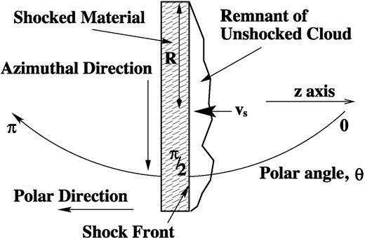
A cartoon of the situation near the end of shock passage through a cloud, viewed parallel to the shock front. In this frame, a small remnant of the unshocked cloud approaches the shock front, which is at rest, at speed vs. The shocked material is approximated as a short cylinder, shown here edge-on as a shaded rectangle. Polar and azimuthal directions are marked, noting that the latter follows the curved edge of the cylinder.
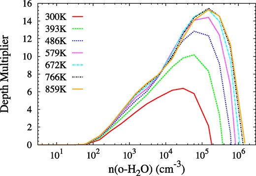
Model optical depth multiplier in the 22-GHz maser transition, τM as a function of |$n_{\rm {o-H_2O}}$|, the number density of ortho-H2O at kinetic temperatures of 300, 393, 486, 579, 672, 766, and 859 K, as used in Gray et al. (2016), and shown in the key. The fractional abundance of o-H2O with respect to H2 is 3 × 10⁻⁵. Values of τM < 0, where the 22-GHz transition is in absorption, are not plotted.
If the maser medium, even after being shocked, hosts only unsaturated masers, then it is relatively straightforward to model the maser emission. However, model turbulence mapping (Strelnitski et al. 2017) compares the expected spectra and maps from a turbulent medium in both the saturated and unsaturated cases. The unsaturated case predicts maps dominated by a small number of spatially isolated statistical outliers with very high maser optical depth, whilst saturated masers tend to form with fractal clustering, and a comparatively small intensity dispersion. The saturated model compares considerably better with observations.
1.3 Other modelling of maser flares
Deguchi & Watson (1989) explained the basis of maser variability by considering changes in the radiation field affecting the background and pumping, or changes in the effective gain length (velocity-coherent amplification path). Such changes due to line-of-sight overlap of slabs and filaments were modelled as the origin of giant H2O maser outbursts in Orion and W49 (Elitzur, McKee & Hollenbach 1991). A model emphasizing the role of J-type shocks in the generation of bright H2O masers, that we do not consider further here, was proposed by Hollenbach, Elitzur & McKee (2013). A magnetohydrodynamic (MHD) shock origin was suggested also for OH masers during a flare in W75N (Slysh, Alakoz & Migenes 2010).
More recent theoretical work on maser flares has diversified considerably. While the current authors consider 3D radiative transfer (RT) models of au-scale maser clouds, including saturation, there are several other approaches. For example, an entirely different explanation for maser flares, Dicke super-radiance has been suggested (Rajabi & Houde 2017; Rajabi et al. 2019). Olech et al. (2020) reconstructed 3D source structure from a combination of VLBI data and time delays between the flaring of individual maser features. Many-model grids have been used to derive physical conditions or pumping schemes explaining flares (e.g. Salii et al. 2022 for CH3OH masers, and McCarthy et al. 2023 for a new maser transition of NH3). An analysis of line widths has been used to link gas motions to turbulence in the source, and to deduce an absence of homogeneous, spherical maser clouds (Krasnov et al. 2015). Where the models above solve the RT problem, they typically use approximations, for example the large velocity gradient (LVG) version of the escape-probability method, or 1D models.
Another group of models seeks to establish the radiation field, as a function of time and wavelength, that is generated by time-dependent processes in the central source, for example colliding binary wind shocks (Parfenov & Sobolev 2014), stellar pulsation (Inayoshi et al. 2013), and unsteady accretion (Araya et al. 2010). An example that computes spectral energy distributions (SEDs) over a wide range of wavelengths from continuum radiation transfer solutions is Stecklum et al. (2021).
There is a useful summary of maser models, not necessarily applied to flaring sources, in the H-atom maser paper by Prozesky & Smits (2020). Mention should be made of the accelerated lambda iteration code magritte (De Ceuster et al. 2020, 2022) that is fully 3D, and may soon have the capacity to study saturating masers with full molecular complexity included.
2 RADIATIVE TRANSFER MODEL
In this section, we briefly describe the model that is used to solve the RT problem for maser radiation, in 3D, at essentially arbitrary degrees of saturation. We keep this separate, as far as possible, from the shock-wave physics (see Section 3) that is used to generate input physical conditions for the RT model. We summarize the key points of the RT model in Section 2.1, before entering a more detailed discussion of how the model has been upgraded from the version used in Paper 3 in Section 2.2. Modifications necessary to model a partially compressed cloud with various fractions of its volume swept by the shock are deferred until Section 3. As in Paper 3, we approximate a time-dependent model as a series of snapshots that are, in themselves, time-independent. The necessary assumption that other processes can relax on time-scales significantly shorter than the snapshot interval is perhaps more easily satisfied in this work because the pumping schemes are collision-dominated, without the added complexity of external sources of pumping radiation. We estimate a suitable minimum snapshot interval in Section 3.3.
2.1 Key points from Papers 1–3
The motivation for the theory and code in Paper 1 was to enable the modelling of ‘real-Universe’ maser clouds, lacking a specified geometry. Possible problems to be considered included natural beaming angles and the influence of cloud shape on maser flares, for example in Paper 2. Model maser clouds in Papers 1–3 and this work are constructed by DeLaunay triangulation from an original point distribution, and represent a single cloud. The code can also operate with compound domains comprising many clouds, but these are not considered further here. Tetrahedra from the triangulation become the basis for a finite-element solution of the combined RT and statistical equilibrium equations for arbitrarily saturated masers in a single transition. Such solutions are 3D generalizations of Schwarzschild–Milne style methods (e.g. King & Florance 1964) in which radiation integrals, particularly the mean intensity, are eliminated analytically to leave integral equations in the inversions. On discretization (e.g. Elitzur & Asensio Ramos 2006 and Paper 1) these become non-linear algebraic equations for the nodal inversions. Input radiation to the model comes from a variable background, and spontaneous emission from the maser transition itself is ignored, as in many maser-focused studies. We therefore solve a set of coupled non-linear algebraic equations of the general form
where |$\delta ^{\prime }_{j} = \delta _j /\delta _{0,j}$| is the fractional inversion at node j of the triangulated domain, situated at position |$\boldsymbol {r}_j$| measured from the domain origin, and is guaranteed to have a value |$0 \le \delta ^{\prime }_{j} \le 1$|. The unsaturated inversion at node j is δ0, j, and this is a function of position, as in Paper 3. The δ0, j have a global scaling, to a reference value, usually |$\delta _{0,\rm {max}}$|, the largest unsaturated inversion at any node of the model. Further details appear in section 2.2 of Paper 3. At |$\boldsymbol {r}_i$|, a total of Q rays converge: each ray has a background intensity iBG, q relative to the saturation intensity, which is the maser intensity that halves the unsaturated inversion, and is defined symbolically in equation (16). Each ray has an associated solid angle element equal to the background sky area, |${\cal A}_q$|, divided by the square of the distance, lq, from the background source to the target node along the ray. Ray q is bounded by J(q) nodes along its path from domain entry to target node. This set of nodes is decided via membership of the elements through which ray q passes on the way to the target. Ray solid angles are almost equal for every ray converging on the target from a background source of ‘celestial sphere’ type. The variable velocity modification in Section 2.2 introduces a numerical frequency quadrature, achieved via a total of K quadrature abcissae, and weights, ζk. The overall saturating effect of the model is controlled by the depth multiplier, τM, essentially a measure of the unsaturated inversion, and the saturation coefficients, |$\Phi _{j,k}^{q,i}$|, that depend on target node, i, frequency abcissa, k, ray, q, and bounding node, j. Note that equation (1) contains no radiation integrals: their effect is exerted through the |$\Phi _{j,k}^{q,i}$|. In its original form, the analytic elimination of the radiation appeared in Paper 1, where a restriction to a static medium allowed us to also analytically integrate over the frequency. A newer derivation of equation (1) appears in Section 2.2.
Once a solution of equation (1) has been obtained at all nodes of the model, comparatively cheap formal solutions of the RT equation may be performed towards an observer, remote compared to the domain size, and in an arbitrary direction. The formal solutions may then be strightforwardly converted to synthetic images and spectra. Frequency channels in formal solutions used to generate our model spectra and images are allocated, unless otherwise stated, such that 25 channels cover 7 Doppler widths. For example, H2O molecules at 670 K have a Doppler width of 0.784 km s−1, so one channel has a width of 0.22 km s−1.
2.2 Variable bulk velocity
The model used in this work is, in many ways, substantially simpler than that used in Paper 3: there are no driving functions to be considered, and uniform density, pseudo-spherical, clouds seem a reasonable approximation to use for the initial state, prior to shock impact. However, a necessary complication is to include a velocity field within the cloud. The aim here is to introduce this velocity variation, whilst maintaining an essential tenet of previous code versions: that saturation can be represented by an array of pre-computed coefficients, the |$\Phi _{j,k}^{q,i}$| in equation (1), that remain constant throughout the iterative procedure that calculates the maser inversions at all nodes of the model (hereafter nodal inversions). The nodes are points within the computational model that are vertices of one or more of the tetrahedral elements generated by triangulation of a 3D structure (see, e.g. fig. 1 of Paper 1).
The theory introduced in section 2 of Paper 1 starts out with equations that are general enough to consider variation in both the internal velocity of the cloud and in the Doppler line width (through variation in kinetic temperature or microturbulent speed). In that work, we subsequently made some more restrictive assumptions in Section 3.1 that included a negligible internal velocity field. Here, we return to equation (11) of Paper 1, the formal solution of the RT equation for the specific intensity as a multiple of the saturation intensity, which we reproduce here,
with the notational change that we use the variable-density inversions, δ′(τ′), as in Paper 3, rather than the original uniform density Δ(τ′). This new inversion scaling is carried through to the gain coefficient in the RT part of the problem, changing the optical depth scale, τ′, in equation (2).
Symbols used in equation (2), together with key stages in its discretization are set out in detail in Appendix A, showing the construction of the saturation coefficients, |$\Phi _{j,k}^{q,i}$|, where the various indices are as introduced in Section 2.1 If the Gauss–Hermite quadrature method is used, with weights ζk and abcissae ϖk, then the discretized mean intensity that has been developed via a frequency and solid-angle average of equation (2) is the final equation of Appendix A, equation (A17). When this result, representing the mean intensity of the maser at the target node, is substituted into the following expression for the fractional population inversion:
we recover equation (1), an example from a set of non-linear algebraic equations in the nodal inversions. Compared with the model in Paper 3, the chief added complexity is the additional index k, corresponding to the frequency abcissae, which raises considerably the memory requirement for the array that stores the coefficients.
3 MODEL CLOUDS
3.1 Compressed clouds
For those models requiring a structural change to the cloud due to shock impact, compressed clouds were constructed from original pseudo-spherical point distributions, and then compressing the z-coordinate for a fraction of the cloud by an amount corresponding to the shock velocity. The algorithm used first calculates Δz, the maximum separation of any pair of nodes along the z-axis of the domain. The z-position of the shock was then computed as z0 = zmin + fsΔz, where zmin is the z-coordinate of the node with the most negative z-position and fs is the fraction of the cloud shocked (by linear distance, rather than volume). For all nodes with a z-position such that z < z0, a modified z-position was computed from
where x is the compression factor imposed by the shock. The partially compressed domain was then triangulated, and density and velocity corrections applied to the file of physical conditions. Densities in the part of the domain with z < z0 were then adjusted to xn0, where n0 is the density in the unshocked material, and the z-component of the velocity was set equal to the shock speed for all nodes in the same part of the domain. Shocked fractions generally run from zero to 1.0 in steps of 0.05, giving 21 points covering the change in cloud structure and approximating to the rise time of the flare, which has an approximate range of 30–300 d. Fig. 1 shows a sketch of a cloud with a large compressed fraction, in which the shocked material is represented as a short cylinder.
Models corresponding to C-type shocks (see Section 3.2.1) retained the original pseudo-spherical point distribution, with the shock affecting only the number density of the maser molecule. This quantity had pre- and post-shock values, and an intermediate zone in z, where the abundance of the maser molecule varied linearly between the two extremes. The overall number density is assumed to vary negligibly over the range of distance where the number density of the maser molecule rises rapidly (Kaufman & Neufeld 1996, fig. 2). Even at the greater distance corresponding to the hottest part of the shock, compression is still said to be less than a factor of 2.
3.2 Simple shock models
The purely geometric considerations introduced in Section 3.1 are now modified in ways that make this work rather specific to collisionally pumped transitions of H2O, and especially the 22-GHz maser transition. There are a small number of model types, set out in Table 1, and these are introduced below in order of increasing sophistication. All of these models are treated as isothermal, and we justify this approximation on the following basis. In the hydrodynamic type, the most important parameter that governs the behaviour of the post-shock gas is the distance Lcool, over which the initially shock-heated gas returns to its pre-shock temperature. For shocks propagating into molecular gas, H2O itself is an important coolant if its abundance is high enough, and the temperature reaches at least 250 K (Tennyson et al. 2016). We consider the cooling time in Draine (2011), equation (35.33):
where the most right-hand version in equation (5) assigns f = 6 degrees of freedom for H2O at temperatures ≲1500 K. In equation (5), n, T, and Λ are, respectively, the number density, kinetic temperature, and cooling function in the post-shock gas. The cooling function for H2O in Tennyson et al. (2016) is in a form per unit solid angle, and per molecule. Multiplication by the number density of H2O and by |$4\mathrm{\pi }$| then places this function in the more usual erg s−1 cm−3. We then find that only the fractional number density of H2O is needed, and using the numerical value of 10−13 for the Tennyson et al. cooling function, the cooling time at 1500 K is |$6600 / f_{-4}$| s, where f−4 is the water abundance with respect to the total number density in multiples of 10−4. The actual cooling time is arguably shorter, since we have not included any other cooling species, though we estimate the contribution of H2 at densities above 106 cm−3 to be considerably lower than that of H2O according to data in Coppola et al. (2016). Models never assume maser-zone H2O abundances below f−4 = 0.1, yielding a maximum cooling time of 66 000 s, or 18.3 h. Converting this to a length via the equation,
we find that the cooling distance is never significantly larger than 1.7 × 10⁵ km for a shock speed of 10 km s−1. As this is vastly smaller than typical internodal spacings in our model domains, we are justified in treating this type of shock, including its cooling zone, as a localized disturbance of infinitesimal thickness. We also always use the approximation of a plane-shock front propagating through a pseudo-spherical cloud, and acknowledge that this ignores the possibilities of both large-scale curvature of the shock front and smaller-scale distortions that may arise from Rayleigh–Taylor and similar instabilities.
Parameters of shock models.
| Model | Comp. | vs | τM | |$\Delta ^0_{\rm {pre}}$| | |$\Delta ^0_{\rm {post}}$| | |$n_{\mathrm{o-H_2O}}$|(pre) | |$n_{\mathrm{o-H_2O}}$|(post) | B(pre) | n(H2) (pre) |
|---|---|---|---|---|---|---|---|---|---|
| (x) | km s−1 | cm−3 | cm−3 | cm−3 | cm−3 | mG | cm−3 | ||
| 0 | 9 | 7.50 | 1.0–5.0 | 3.63–18.15 | 32.67–163.35 | X1 | Y2 | 0.0 | (5.13–25.7) × 106 |
| 1t | 9 | 4.60 | 1.0–10.0 | 3.63–36.3 | 20.13–54.27 | (1.54–102)× 102 | (1.39–91.8)× 103 | 0.0 | (5.13–340)× 106 |
| 2t | 16 | 6.14 | 1.0–10.0 | 3.63–36.3 | 23.33–53.03 | (1.54–102)× 102 | (2.46–163)× 103 | 0.0 | (5.13–340)× 106 |
| 3t | 25 | 7.67 | 1.0–10.0 | 3.63–36.3 | 26.24–51.44 | (1.54–102)× 102 | (3.85–255)× 103 | 0.0 | (5.13–340)× 106 |
| 4v | 11.8–31.4 | 15–40 | ∼0.0 | ∼0.0 | 61.98 | 3.0 | 1.50 × 10⁴ | 10.0 | 5.0 × 10⁷ |
| 5v | 11.8–31.4 | 15–40 | ∼0.0 | ∼0.0 | 82.52 | 6.0 | 3.00 × 10⁴ | 14.1 | 1.0 × 10⁸ |
| 6v | 11.8–31.4 | 15–40 | ∼0.0 | ∼0.0 | 90.80 | 12.0 | 6.00 × 10⁴ | 19.9 | 2.0 × 10⁸ |
Notes. Columns numbered from left to right are: (1) model number, (2) compression factor, (3) shock speed, (4) maser depth of the unshocked cloud, (5) and (6) inversion number density in pre- and post-shocked gas as marked, (7) and (8) number density of ortho-H2O in the pre- and post-shock gas as marked, (9) pre-shock magnetic flux density, and (10) pre-shock number density of H2. Subscript |$\rm {t}$| specifies a model depth from {1, 2, 3, 4, 5, 6, 8, 10}. Subscript |$\rm {v}$| specifies a shock speed in km s−1 from 15 to 40, inclusive, in steps of 5. Note that figures in column 10 are unchanged after passage of the H2O abundance front and compression factors from column 2 should be applied only to obtain ultimate H2 number densities after momentum transfer to the neutrals.
This type of hydrodynamic shock has a jump in physical conditions almost immediately behind the shock front, and we approximate the compression factor by |$x = M_0^2$|, where M0 is the Mach number, given by vs/viso, the ratio of the shock speed to the isothermal sound speed. This model type corresponds to strong coupling between the ion and neutral fluids, as might be the case for magnetic fields that are abnormally weak compared to the predictions of the relation defining b (Kaufman & Neufeld 1996), where b is in the range 0.1–3, or to a higher than typical fractional ionization. Typical values of nH, the number density of H-nuclei, lie in the range 106–108.5 cm−3 in the pre-shock gas.
In the very simplest model, we use the compression factor above, and make the naive assumption that the unsaturated inversion itself follows the overall density compression. This amounts to allowing the shock to generate a fresh supply of H2O molecules. This simplest model is implemented as Model 0. Models of the form Model N, where 0 < N ≤ 3, adopt a constant fractional abundance of the maser species, and consider the consequences of the increased post-shock density on the maser pumping scheme, based on the more sophisticated analysis described below. We defer an additional discussion of the C-type models (3 < N ≤ 6), where the abundance of the maser molecule is variable, to Section 3.2.1. The important parameters of all models are listed in Table 1.
In all our shock model types, an important computational parameter is the optical depth multiplier, τM, a dimensionless representation of the inversion in a specific transition of the maser species. The parameter τM relates the inversion to the dimensioned cloud size, R. Specification of τM and R leads directly to the dimensioned unsaturated inversion, Δ0, (in cm−3) in the unshocked gas, since
which is derived by setting the scaled radius of the original unshocked cloud to τM, so that τM = Rγ0, where γ0 is a gain coefficient. Other parameters include the velocity width W, a constant in the isothermal model, the transition wavelength λ0 and Einstein A-value, A, and the upper-state statistical weight, gu. The second expression on the right-hand side of equation (7) uses the parameters of the 22-GHz transition of ortho-H2O with the scaled parameters T400, the kinetic temperature in units of 400 K, Rau, the cloud radius in astronomical units and Δcc, the 22-GHz inversion in cm−3.
Data in Gray et al. (2016) show that the relation between the inversion and the overall number density of the maser species is complicated, and only in a naive model could we take the inversion to be simply a fixed fraction of the species number density. Assuming that the maser species is ortho-H2O, then while τM is simply related to the inversion via equation (7), we need to establish a more complicated relation between τM and |$n_{\rm {o-H_2O}}$|, the number density of ortho-H2O. We do this in the following way: The maser depth in Gray et al. (2016) is related to the mean gain coefficient, 〈γ〉 via τ = z〈γ〉, where z is the slab thickness, and 〈γ〉 is related to an inversion per unit bandwidth at line centre, Δ0, ν, via the equation from Yates, Field & Gray (1997)
Using the value of the Gaussian molecular response at line centre, we then find |$\Delta ^0 = \mathrm{\pi }^{1/2} W \Delta ^{0,\nu } / \lambda _0$|, and the optical depth in the 3D model is
which reduces to τM = 0.871τRau for the 22-GHz transition. It is now possible to draw a line at constant temperature through the data underlying the 22-GHz panel of fig. 5 of Gray et al. (2016), yielding directly τ as a function of |$n_{\rm {o-H_2O}}$|. This relation can then be converted to τM as a function of |$n_{\rm {o-H_2O}}$| through equation (9). We plot the relation between τM and |$n_{\rm {o-H_2O}}$|, for a number of kinetic temperatures, in Fig. 2. The curves in this figure incorporate, in principle, all the complexity of the pumping scheme for the 22-GHz transition, and it is apparent that, while τM rises at modest values of |$n_{\rm {o-H_2O}}$|, there is also a decaying part of each curve, dominated by collisional quenching of the inversion at high density. It is also apparent from Fig. 2 that for kinetic temperatures above ∼500 K, the curves are not strong functions of temperature, particularly on the low-density side of the peak.
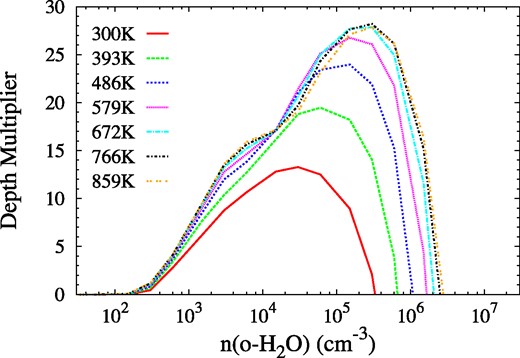
As for Fig. 2, but for a higher fractional abundance of ortho-H2O, equal to 3 × 10⁻⁴ with respect to H2. The parameter τM, the depth multiplier, is a measure of the available population inversion in the 22-GHz transition.
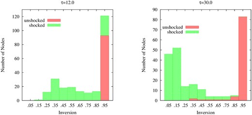
Inversion distributions amongst 10 bins for depth multipliers of τM = 12 (left panel) and 30 (right panel) for a cloud in which a shock of compression factor 9 has passed through half the z-extent of the material.
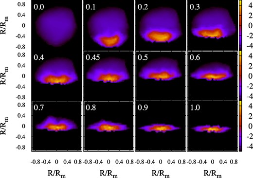
A sequence of images showing the maser brightness distribution varying as the shock progresses through the originally pseudo-spherical cloud. The number at the top left of each panel is the fraction, f, of the z-axis extent of the cloud that has passed through the shock. The z-axis itself points vertically from the bottom towards the top of each panel. The scale bars to the right of each row show the base-10 logarithm of the specific intensity in units of the saturation intensity of the maser. Note that there is a frame change at f = 0.5: at earlier times, the shock is shown moving in the positive z-direction into the cloud. at later times, the shock is shown stationary at z = 0, while the remnants of the cloud flow into it in the negative z-direction. This shift is purely for the viewer’s convenience.
The practical procedure for the use of Fig. 2 is to take the value of τM for the unshocked cloud and continue it to an intercept with the curve of appropriate temperature, reading off the corresponding |$n_{\rm {o-H_2O}}$| from the x-axis. The shock compression factor x is then applied to |$n_{\rm {o-H_2O}}$|, noting that this is taken to be a constant fraction of the number density of H2 in Models 1–3, but varies in the C-type models, 4–6 that use Fig. 3 instead (see Section 3.2.1). The value of |$n_{\rm {o-H_2O}}$| in the compressed gas is then continued to the correct curve, in order to obtain τM in the shocked gas. All models except Model 0 apply the practical procedure described above, to limit the post-shock inversion (or τM) in line with expectations of high-density collisional quenching.
3.2.1 Continuous model
Our remaining models, 4–6 in Table 1, draw heavily on the continuous (C-type) shocks described in Kaufman & Neufeld (1996), where physical variables change smoothly across the shocked portion of the cloud. The only physical parameter that changes rapidly (over ≃0.5 au) in these models is the H2O abundance, and we treat this as the ‘shock front’ in our models. We do not consider details of chemistry in the post-shock gas, and rely on the results in Kaufman & Neufeld (1996) for H2O abundances (relative to the H2 number density unless otherwise stated) as necessary. In continuous models, the compression factor, x, is achieved only after a long process of momentum transfer from the ionized to the neutral fluid, and x is related to the shock speed via the Alfvénic Mach number, MA. For an isothermal shock where the isothermal Mach number, MISO, is much larger than MA, and both Mach numbers are >1, the ultimate compression factor is |$x=\sqrt{2} M_{\rm {A}}$| (e.g. Draine 2011), for a magnetic field in the plane of the shock. The Alfvénic speed in km s−1 is given by
(Kaufman & Neufeld 1996) where b is a constant in the approximate range 0.1–3.0. However, b ≳ 1 is generally required by the requirement of MISO > MA. The magnetic flux density in the pre-shock gas is
where nH is the pre-shock number density of hydrogen nuclei. For our models 4–6, equation (11) leads, respectively, to B = 10, 14.1, and 20 mG.
Momentum is transferred from ions to neutral particles over the distance Lmt. We consider extremes for this distance via the equation
where we have used equation (10), and we derive values of the ion-neutral coupling length, Lin from fig. 1 of Kaufman & Neufeld (1996). Equation (12) yields the shortest Lmt for the maximum pre-shock density and highest shock speed. We use the shock models that include populations of large charged (polycyclic aromatic hydrocarbon, PAH-type) molecules, and small dust grains: the alternative yields values of Lin and Lmt that are so large that physical conditions vary so little across a cloud of a few au in diameter that these models are not useful for the generation of flares. With the PAHs and grains, the densest pre-shock models in Kaufman & Neufeld (1996) (nH = 2 × 109.5 cm−3) correspond in their fig. 1 to Lin ∼ 1014.3 cm. With this distance, b = 0.1, the smallest value considered, and a shock speed of 40 km s−1, the upper limit for an unambiguous C-shock, we obtain from equation (12), the smallest reasonable momentum-transfer length of Lmt = 9.0 × 1011 cm (0.06 au). This distance is so short compared to the cloud scale that one could reasonably treat the entire shock as a thin disturbance, and use a model similar to the hydrodynamic types discussed above. By contrast, the lowest density used by Kaufman & Neufeld (1996), where nH is equal to 2 × 107 cm−3, corresponds to the much larger Lin of 1015.55 cm (236 au), and the largest reasonable value of Lmt (with b = 3 and a 15 km s−1 shock) of 85 au. The C-shock paradigm therefore spans a range of momentum-transfer scales from a regime small enough to be treated as a discontinuity, at the resolution of our maser models, to scales much larger than typical flare-supporting clouds (0.5–2 au in asymptotic giant branch stars, 6–9 au in red supergiants: Richards et al. 2012, and ∼1 au in star-forming regions: Uscanga et al. 2005 and further examples in Section 1.1). We resolve this issue in part by noting that at n(H2) = 109.5 cm−3 and an ortho-H2O fraction of 3 × 10⁻⁴ (modest for the models in Kaufman & Neufeld 1996) |$n_{\rm {o-H_2O}} =9.5\times 10^5$| cm−3, and the 22-GHz inversion is already entering the quenching zone on the right-hand side of Fig. 3 for temperatures >400 K. This figure is an analogue of Fig. 2 for an order of magnitude higher H2O abundance. To obtain strong inversions, we adopt n(H2) close to 108 cm−3, and here we find Lmt = 3.9 au for a 35 km s−1 shock, favouring a model where all quantities except the H2O abundance change only slowly within an au-scale cloud. This view is reinforced by examining fig. 2 of Kaufman & Neufeld (1996). We note that significantly larger H2O maser cloud sizes have been estimated from observations. for example, 0.6–14.5 au in S140-IRS (Asanok et al. 2010), but these are not necessarily associated with flares.
With the above considerations, we adopt the following C-type model: the passage of the H2O abundance front causes no deformation of the cloud structure and leaves a constant overall number density. The velocity of neutral species is close to constant, but we allow a small velocity gradient, in line with fig. 2 of Kaufman & Neufeld (1996), of 10 per cent of the shock velocity over 0.5Lmt. The kinetic temperature is set to a constant value of 672.41 K. Obviously, this is incorrect for the pre-abundance-front gas, but for a maser model the value here is irrelevant, since the H2O abundance is approximately 5000 times smaller in this material, when compared to the post-abundance front gas. After passage of the abundance front, we justify the constant number density on the grounds that the generated inversion does not depend strongly on TK for temperatures >400 K (see Fig. 3), and any temperature-dependent effect is dwarfed by that due to the abundance rise in o-H2O by over three orders of magnitude. This abundance rise is assumed to occur exponentially over a transition zone of thickness |$0.5 (35/v_{\rm {s}} \mathrm{km\, s^{-1}})$| au. In Kaufman & Neufeld (1996), the abundance of H2O is expressed relative to oxygen atoms not bound in CO. However, since the same work assumes that CO is the only reservoir of gas-phase carbon, it is straightforward to convert this to an abundance relative to H2. Conversion of free oxygen to H2O is essentially complete for vs > 15 km s−1, see fig. 4 of Kaufman & Neufeld (1996), leading to abundances as large as 8.5 × 10⁻⁴. In our models, we use the more conservative value of 4.0 × 10⁻⁴ so that, assuming a 3:1 abundance ratio of ortho- to para-H2O, our abundance of o-H2O is 3.0 × 10⁻⁴. Our figure is consistent with the post-shock H2O abundance of 3.5 × 10⁻⁴ found by Melnick, & et al. (2000) for Orion KL.
3.3 Applicable time-scales
The basic time-scale that governs the models used here is the shock crossing time of the original cloud, or ts = 2r0/vs, where r0 is the radius of the original pseudo-spherical cloud and vs is the shock speed. It is convenient to measure the cloud radius in au, and the shock speed in multiples of 10 km s−1, and in these units, the crossing time in days is
As the light-crossing time is of order 30 000 times shorter, we can assume, with greater confidence than in Paper 3, that radiation transfer is set up on a much shorter time-scale than ts, even if the pumping scheme of the maser depends on some transitions that are substantially optically thick. As a justification, we use, as in Paper 3, estimates of optical depths of 350–1000, for an au-scale cloud, in the ‘sink’ transition, at 53.1 μm, from the o-H2O spin species that is an important part of the pump for the 22-GHz maser transition, see for example de Jong (1973). Even at the upper end of this optical depth range, the photon diffusion time, of order the optical depth multiplied by the light-crossing time, is still 30 times shorter than ts, and is approximately 12 d. Since both time-scales include a crossing time, use of a larger cloud does not increase the ratio of the diffusion time to ts unless the optical depth also increases substantially. If we appeal to effective scattering to reduce the diffusion time, as in Paper 3, the model can at least be a starting point for discussion for time-scales as small as 1.2rau d, where rau is the cloud radius in astronomical units.
In all cases where the shock can be counted as a thin disturbance within the approximations of our model, the time-scale ts from equation (13) is the only one that governs the rise of the flare. However, in a continuous shock, the momentum-transfer time and the associated ion–neutral coupling time are also important, to the extent that they may far exceed the time that is considered suitable for the initial rise of a flare. To the best of the knowledge of the current authors, there is no formal definition that separates times appropriate for a spectacular flare from those that represent some gentler form of variability. From the observations considered in the Introduction, an approximate upper limit for what might be considered a flare is perhaps of order a few years. Therefore, in our C-shock models, which cannot be considered thin, there may be substantial post-flare evolution as the cloud becomes cooled, compressed and the neutral velocity approaches vs. The initial enhancement time of H2O in the C-shock models can be estimated by dividing the thickness of the transition zone from Section 3.2.1 by the shock speed. The result is
Our models are generally considered complete when either the shock front (in hydrodynamic models) or the H2O abundance front plus its transition zone have passed completely through the cloud. Therefore, models have a duration of approximately ts. The time taken for the radiation flux density to rise from the pre-shock level to its maximum may differ somewhat from ts. We do not attempt to model in detail the further evolution and decay of the flare, but we make the following observations here. For hydrodynamic models, if the pre-shock cloud was in approximate pressure equilibrium with its surroundings, then the shocked cloud will be considerably overpressured because of its enhanced density. If we need to model the decay of a flare of this type, we use a simple exponential recovery of the overpressured gas towards the original pressure, of the form |$e^{-t/\tau _{\rm d}}$|, where τd is a dynamical time. For τd, we use,
where cs is the sound speed in the shocked gas, and Lz is the z-axis thickness of the shocked cloud once shock passage is complete (shocked fraction = 1.0). It is most unlikely that the compressed cloud will relax back to anything resembling its original shape.
If the flare decay is very uncertain in the hydrodynamic case, it is much more so for the C-type shocks. The compressive evolution, over a time >Lmt/vs introduced above, may enhance the flare for mild density increases, but could also destroy the inversion through quenching as x approaches its ultimate value. Cooling to temperatures <400 K is also detrimental to the 22-GHz inversion (see Fig. 3), and such cooling accompanies compression in the models by Kaufman & Neufeld (1996). A final dissolution of the cloud may then occur on a time-scale found by substituting vA for cs in equation (15), where vA is the post-shock Alfvén speed. However, it is quite possible that the magnetic field, oriented in the plane of the shock front, may inhibit to some extent any relaxation flow in the z-direction.
3.4 Notes on pumping variability
All our models treat the gas as isothermal. Variability therefore depends entirely on changes in density and/or abundance. We also expect that none of the shocks we consider will dissociate H2O, so that the fractional abundance of water will remain approximately constant throughout the cloud in the hydrodynamic models, and will rise quickly to a constant value in the C-type models. The original cloud in a hydrodynamic model is therefore already a potential maser, since no external radiation is needed to drive the standard ‘collisional’ pumping mechanism for the 22-GHz transition of H2O. The original cloud could even be an observable VLBI maser feature, though probably rather a weak one. With this in mind, the kinetic temperature may change significantly across the shock, but the pre-shock value is not very important because the unshocked gas provides only a very small fraction of the maser flux density during a flare.
The appearance of the shock may increase the brightness of the maser in two ways, one of which depends on the viewpoint of the observer, and the other which does not. The view-independent effect of the shock is that it may increase the available inversion through a combination of increased |$n_{\mathrm{o-H_2O}}$| in the shocked material, and an increased efficiency of the pumping mechanism. This increased efficiency is based in Elitzur et al. (1989) on the enhanced escape probability for line pumping radiation in directions perpendicular to the maser propagation direction in cylindrical and filamentary masers, relative to spheres. The combined effect may be estimated from, for example, fig. 5 of Gray et al. (2016), where a compression of a factor of 10 at a kinetic temperature of ∼700 K could shift the number density from 104–105 o-H2O cm−3 (for the standard fractional abundance, corresponding number densities of H2 are 3.3 × 10⁸ and 3.3 × 109 cm−3). This number density increase raises the maser depth in that model from approximately 7 to 17, a factor of considerably less than that in the number density itself. This supports the view that we should not simply use the number density as a proxy for the initial inversion. Over a given length, if the maser remained unsaturated, a single ray of the maser would become brighter by a factor of e10, or 22 000 based on the raw number density of o-H2O, but only by e17/7 (11.34) based on the maser depth that depends only on the number density of inverted o-H2O molecules, modelled as nodal inversions. As the shock advances, more of the cloud becomes enhanced in o-H2O, and angle-averaged quantities, such as the flux density would also be expected to increase.
The pre-shock number density is crucial: too high and the post-shock o-H2O number density may be past the optimum masing conditions, corresponding to the peaks in Figs 2 and 3, and into the quenching zones on the right-hand sides of these curves, where the 22-GHz transition falls rapidly into absorption. If the initial number density is too low, the maser may brighten, but is unlikely to be considered observationally spectacular.
The viewpoint of the observer is also very important in a shock model. Although the specific intensities and flux densities received by an observer depend in a complicated way on the passage of many competing rays through a cloud, an important parameter is the velocity-coherent column density of molecules of the maser species along a given ray, and this is directly affected by the shock. Perpendicular to the shock front, the amount of material along a ray is approximately the same as in the original cloud, independently of the distance the shock has penetrated into the cloud. However, the velocity coherence is reduced by the velocity change due to the shock. By contrast, rays moving parallel to the shock front within the post-shock gas experience little change in velocity coherence, while the overall column density of the maser species rises due to the higher post-shock number density. Providing this post-shock density is not high enough to quench the inversion, we therefore have a basic expectation that the brightest rays will be emitted towards an observer viewing the cloud parallel to the shock front.
3.5 Parameter ranges
The most important parameters of the models considered in this work are displayed in Table 1. The standard isothermal kinetic temperature used was 672.41 K, corresponding approximately to the temperature that generated the maximum maser depth in Gray et al. (2016). Subscripts on a basic model number correspond to a final, or target, value of τM. Generally, we increase τM from a starting value of 0.1 (optically thin and unsaturated) to the target value in steps of 0.1. Model 0 is special in this respect, because the solution at every value of τM is a valid model, rather than just a numerical staging point on the way to the target value. The maximum τM used in Model 0 was 5.0, corresponding to significant saturation, and a large value of the inversion.
All hydrodynamic models, including Model 0, use an abundance ratio of o-H2O to H2 of 3.0 × 10⁻⁵ to agree with the models in Gray et al. (2016). For Models 1–3, the target τM values correspond to pre-shock number densities of ortho-H2O between 60 and 3.75 × 104 cm−3. The compression factors of 9, 16, and 25 are applied to these pre-shock number densities, but are applied to the inversion only in Model 0. Post-shock inversions in Models 1–3 are limited via consideration of Fig. 2. The maximum value of the pre-shock o-H2O number density (or of τM) corresponds approximately to the boundary of the quenching zone in the post-shock gas, beyond which models are uninteresting from the point of view of generating flares.
C-type models (4–6) have a subscript that specifies the shock velocity (from 15 to 40 km s−1). Within one model, the post-shock o-H2O number density follows immediately from the pre-shock H2 number density and our standard fractional abundance for these models of 3.0 × 10⁻⁴. The pre-shock abundance of o-H2O is small (1/5000 of the post-shock value). As the H2 number density is considered unchanged by the passage of the H2O abundance front, there is just one target value of τM, based upon the post-shock abundance of o-H2O. The b parameter from equation (10) is 1.0.
4 RESULTS
4.1 Important results from Papers 1–3
We summarize the observational characteristics of flares from previously studied mechanisms as follows:
Rotation of non-spherical clouds, studied in Paper 2, can have variability indices in the range of thousands if the observer’s line of sight is near optimal, but indices of tens are typical for a randomly chosen line of sight. For a pseudo-spherical cloud, see Paper 1, the variability index is only of order 3. Periodicity is unlikely owing to stability considerations.
Radiatively driven flares, considered in Paper 3, are generally more powerful, with variability indices due to pumping variations typically in the range of thousands to tens of thousands. Extreme cases, corresponding to small, unsaturated, initial maser depth (negative optical depth), and large depth change produce variability indices exceeding 105 (107) for oblate (prolate) clouds with an optimal line of sight. Periodicity in this mechanism naturally follows that of any source of pumping radiation, and a similar comment may be made regarding variability of background radiation.
Flares due to variations in the level of the background radiation have somewhat lower variability indices, typically hundreds to thousands, and are also limited by the variability index of the background itself. This type of flaring also has a characteristically long duty cycle.
Cloud overlap in the line of sight can cause flares with a variability index of >50 from observations (in W Hya, Richards et al. 2012). Time-scales are approximately Dau/v10 in years, where Dau is the cloud diameter and v10 is the velocity component perpendicular to the line of sight in km s−1. Such flares are unlikely to be periodic unless there is some favourable cyclic or orbital arrangement.
From the list above, another useful discriminator between the various flare processes is the ability to generate periodic and quasi-periodic flares. There are many other possible styles of maser variability (Goedhart, Gaylard & van der Walt 2004). The duty cycle is also a strong discriminator between flares generated by variable pumping and variable background radiation (Paper 3). For the shock-driven flares studied in this work, we consider periodicity unlikely for individual clouds, because of the fundamental structural change inflicted by the shock passage. However, the geometry of flaring sources could produce quasi-periodic flares if a shock passes through multiple regions each containing many clouds. Periodic flares may also be generated from the CSEs of evolved stars, where periodic pulsation shocks sweep a distribution of clouds that has statistically similar properties from one pulsation to the next, provided that there is a continuous supply of outflowing gas from the stellar photosphere that can renew the cloud population.
The maser beaming angle may also be useful in distinguishing shock-driven flares from other types. A beaming angle related to the diameter-to-length ratio of the maser was introduced by Elitzur et al. (1989), where the H2O masers in star-forming regions are modelled as long, thin cylinders. In evolved star atmospheres, approximately spherical maser clouds were distinguished from the shock-flattened variety on the basis of the frequency dependence of the observed angular size of maser features (Richards et al. 2011). Unshocked clouds have an apparent angular size that is smaller than that of the whole cloud (they are ‘amplification bounded’) and the apparent size depends on the intrinsic beaming angle of the maser. Moreover, the beaming angle depends on chords of amplification through the cloud, and amplification is in turn frequency dependent. By contrast, a shocked cloud, if it presents a fairly flat face to the observer, presents its full cross-section at any frequency (it is matter, or size, bounded).
All solutions are computed from equation (1), noting that the coefficients for each target node, ray, ray-bordering node, and frequency abcissa do not change during iteration, and may therefore be pre-computed, given sufficient memory. A numerical integration over the frequencies is necessary in this work, whilst an analytical form could be used in Papers 1–3. A solution takes the form of a list of saturated inversions, one for each model node. The inversions are on the δ′ scale, that is measured relative to the unsaturated inversion in the individual node, so that 1.0 means unsaturated and 0.0 implies ultimate saturation. A saturated inversion of 0.5 at a node corresponds to the case where the mean intensity there is |$\bar{J} = I_{\rm s}$|, where the saturation intensity, Is is defined as
and the mean intensity is an average over both frequency and solid angle. The rest wavelength of the maser transition and its Einstein A-value are λ0 and A respectively, and the loss rate, Γ, is taken to be independent of pre- or post-shock conditions. For the 22-GHz H2O transition, the statistical weights are gi = 13 and gj = 11. The loss rate has previously been defined in equation (A5) of Paper 3, where Z is used for the loss rate. The change to Γ in this work is purely a notational change. The loss rate is not trivial to calculate, and involves summing a subset of the larger Einstein A-values and rate coefficients out of the upper energy level of the chosen maser transition. Details may be found in Appendix B. The overall method of calculating Γ is the same as that used in Paper 3.
4.2 Comparison with previous versions
To demonstrate that results of the new code converge with those of the old, we compare a run of the old code, which necessarily has zero velocity (meaning all model nodes are stationary with respect to each other), against two runs of the new code, as detailed in Section 2. In the runs of the new model, the 250-node domain had an internal subthermal velocity that varied linearly along the z-axis, such that, in moving from a node with a scaled z-position of −1 to one at + 1, the velocity increased from −v to +v, where v is one of the values in the first column of Table 2. Input parameters for the old and new models were otherwise the same. All of these models were run to a depth-multiplier of τM = 30. The saturated inversions on the δ′ scale at three randomly chosen nodes, numbered 9, 67-, and 225, for three models are shown in Table 2. It is not entirely trivial to run jobs at velocities that are as close to zero as those in Table 2, because the expressions for the saturation coefficients in equation (A14) become inaccurate as the β denominators approach zero. We therefore use a version of the coefficient |$\Phi _{j,k}^{q,i}$| Taylor-expanded to second order in small βqj in this situation, the modified formula being
Saturated inversions at three randomly chosen nodes in τM = 30.0 models for velocities as shown.
| Velocity | Node 9 | Node 67 | Node 225 |
|---|---|---|---|
| (km s−1) | |||
| 0.02 | 0.021911 | 0.019843 | 0.031152 |
| 0.01 | 0.020539 | 0.018703 | 0.030100 |
| 0.00 | 0.020514 | 0.017699 | 0.027527 |
| Velocity | Node 9 | Node 67 | Node 225 |
|---|---|---|---|
| (km s−1) | |||
| 0.02 | 0.021911 | 0.019843 | 0.031152 |
| 0.01 | 0.020539 | 0.018703 | 0.030100 |
| 0.00 | 0.020514 | 0.017699 | 0.027527 |
It was found that a transition value of βqj = 10−7 gives a smooth transition between the full formula and the approximation in equation (17).
4.3 Nodal solutions
Computation of nodal solutions follows the methods used in Papers 2 and 3, with the same non-linear equation solver: the Orthomin(K) algorithm (Chen & Cai 2001) with order K = 2. Unless otherwise stated, depth multipliers were increased in steps of 0.1 from τM = 0.1 to 30.0 for each domain. Complete velocity redistribution, provided by largely isotropic infrared (IR) radiation (Goldreich & Kwan 1974; Frisch 1988; Field, Gray & de St. Paer 1994; Gray 2012) was assumed throughout. The example here uses Model 0 from Table 1.
The new factor introduced by variable velocity is the extent to which saturation might be biased to nodes in either the pre- or post-shock zones of the domain. We therefore plot in Fig. 4 histograms of the distribution of nodal populations for ten bins, marking the contribution of the two zones in each case. In the left-hand panel, we show a case of moderate saturation, and on the right, for the most saturated solution (τM = 30.0) for the same model, in which the shock has penetrated half way through the z-extent of the cloud.We note that half the z-extent is not the same as half the nodes, and that this model has more than half its nodes in the shocked region.
A strong result is that highly saturated nodes (remaining inversion <0.5) are concentrated in the shocked part of the domain. This result is not confined to the example shown here and is more extreme in less saturated models (e.g. the left-hand panel compared to the right-hand panel in Fig. 4).
4.4 Sample images and light curves
We select a low depth multiplier of τM = 3, corresponding to rather weak saturation in the unshocked part of the cloud, and plot a sequence of modelled images (Fig. 5) and light curves (Figs 6 and 7). Distances along the z-axis are represented as fractions of the original z-axis extent of the cloud in Figs 5 and 7, ranging from 0.0 to 1.0 in steps of 0.1 for the images and 0.05 for the light curve. In Fig. 6, the z-axis distance is represented as a time from initial shock impact, based on a shock-crossing time of 463 d for the original cloud. The y-axis values in Fig. 6 are linear, whilst those in Fig. 7 are logarithmic to show the initial rapid rise to good effect. Fig. 6 also shows exponential decays, based on a relaxation time of 126 d, in accord with equation (15) with L equal to R/9 and sound-wave crossing. In fact, both Figs 6 and 7 show two versions of the light curve: one is based on the maximum brightness, Imax, found in any pixel of the images in Fig. 5, in multiples of the saturation intensity, and comparable to the highest specific intensity found in an interferometer image. The other is based on the maximum flux density in a simulated single-dish spectrum, Fmax, and corresponds to an integral over the solid angle of the source. The flux density scaling is explained in the caption of Fig. 7. If the maser source is amplification bounded (Elitzur et al. 1992), then these two representations are related through the relation Fmax/Imax = ΩMl2/d2, where ΩM is the beaming solid angle of the maser, l is the intrinsic size of the maser source, and d, its distance from the observer.
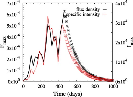
Light curve of the same model as in Fig. 7, but with linear y-axes and added exponential decays (curve sections plotted in symbols). The x-axis has been converted to time, based on a shock-crossing time for the original cloud of 463 d.
Logarithmic light curves for the maximum flux density in any spectral channel (heavy, solid line and left-hand y-axis scale), and the maximum brightness in any image pixel (lighter, dotted line and right-hand y-axis scale). The brightness is scaled to the saturation intensity of the maser transition. The flux density scale results from using a background brightness of 10−6 with respect to the saturation intensity and placing the observer at a distance of 1000 domain units, yielding a background level of |$\pi \times 10^{-12}$|.
The compression factor is 9, and in this model (Model 0), it is the same for the unsaturated inversion. The shock velocity is 7.5 km s−1 in the z-direction. With this velocity, the shock would pass completely through a cloud of original radius 1 au in 463 d from equation (13). From Fig. 7, it is easy to see that a very rapid rise in the light curve, to within an order of magnitude of the eventual maximum, occurs within about 10 per cent of the total crossing time, or 46 d. Shock passage can therefore generate flares with rise times of order 1 month, as has been observed from some sources, for example G25.65 + 1.05 (Shakhvorostova et al. 2018). There is then a substantial plateau, filling the rest of the crossing time. The eventual maximum in the brightness occurs when 60 per cent of the cloud has been shocked. The flux density peaks only after the entire cloud has been shocked.
In terms of the specific intensity, the flare is spectacular: the maximum brightness in the central frequency channel in the original cloud is 2.1 × 10⁻⁴ of the saturation intensity; the eventual maximum is 33 000 times the saturation intensity, yielding a brightness gain of 1.57 × 10⁸ over the unshocked cloud. To convert to an absolute brightness temperature, we calculated the saturation intensity for the 22-GHz transition from equation (16), following the methods in appendix A of Paper 3 and using the parameter values in Appendix B of this work. We then equated our value of Is to the specific intensity from a blackbody in the Rayleigh–Jeans limit in order to obtain the brightness temperature corresponding to Is, which we found to be |$T_{B,\rm {sat}}=2.18 \times 10^{8} I_{\rm s}/ \Omega _{\rm M}$| K. With the 33 000 gain over this temperature, TB at the peak of the flare is 7.20 × 10¹² (ΩM)−1K. A beaming solid angle, ΩM is still required to compare TB to the brightest 22-GHz H2O masers known, for example TB > 1016 K (Kobayashi et al. 2000) or 8 × 10¹⁷ K (Strelnitskii 1982) for a flare in the Orion source.
A great advantage of a 3D model is that it is straightforward to compute an absolute single-dish flux density once the saturation intensity is known. Our version of equation (A6) of Paper 3 for the 22-GHz H2O transition and the current number density in the shocked gas is
where fν is the flux density with the scaling on the left-hand y-axis in Fig. 7, Rau is the original cloud radius in astronomical units and dkpc, its distance in kpc. Since the peak value of fν attained in Fig. 7 is 6.351 × 10⁻⁴, an au-scale cloud at a distance of 1 kpc would yield a flux density of 46.4 Jy. The shock mechanism is therefore capable of lifting a single cloud from complete obscurity to easily observable.
Another notable feature of Fig. 5 is that during the flare the area contributing very high brightness rays to the observer quickly becomes much smaller than the original cloud. To quantify this, in the bottom right panel, where f = 1.0, the fraction of the area that contributes half the total flux density in the brightest spectral channel is only 5.51 × 10⁻³. Another way of putting this is that half the flux density is emitted by just 2 of the 363 rays, or pixels, allocated in the formal solution. Since the overall emission comes from an area of approximately |$\pi$| square astronomical units, half the emission then emanates from an area of |$(2/363)\pi$| (au)2, with a corresponding linear scale of 0.13 au. This is similar in size to the compact halo structure detected by RadioAstron towards Cepheus A (Sobolev et al. 2018). Spectrally, in the model from the last frame of Fig. 5, the central channel contains 0.7473 of the total flux density, and this is typical of models with a substantial fraction of the cloud compressed.
4.5 Density and saturation
We begin by studying the effect of saturation, as imposed by the significant density increase in the shocked part of the cloud. We assume here a close-to-optimum observer’s viewpoint, where the line of sight from cloud to observer is parallel to the shock front. However, we now also consider the more sophisticated Models 1–6 (see Table 1) where the post-shock inversion is limited, and does not simply follow the post-shock density as it does in the simplest model (Model 0) that has been discussed in Section 4.4.
In Models 0–3, we use the model optical depth in the unshocked gas as a proxy for the number density of inverted molecules, that is the difference of the upper- and lower-state populations of the maser transition, divided by their respective statistical weights. The model optical depth and the number density of molecules of the maser species are related through the graph in Fig. 2. In Models 1–3, the graphs from Fig. 2 and the shock compression factor then determine the inverted number density in the post-shock gas and the likelihood of saturation in the resulting maser. In Models 4–6, graphs from Fig. 3 and the shock velocity serve much the same function. Therefore, unlike Model 0, each of the other models can contribute only one point per subscripted version to the graphs in Fig. 8, for Models 1–3, or to Fig. 9 (for Models 4–6). For Model 0, where the inversion follows the overall density, the single model can provide data at all the depths sampled in the upper curves of Fig. 8.
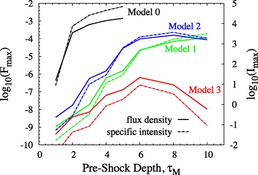
Flux density in the brightest spectral channel (left-hand y-axis and solid lines) and the specific intensity in the brightest map pixel (right-hand y-axis and chained lines). Pairs of graphs are for Models 0 to 3 as marked; colour coding is black (Model 0), green (Model 1), blue (Model 2), and red (Model 3). Scalings are as for Fig. 7. Values are taken for the brightest epoch found in the light curve (see the main text) and may differ between the flux density and specific intensity graphs for a particular model.
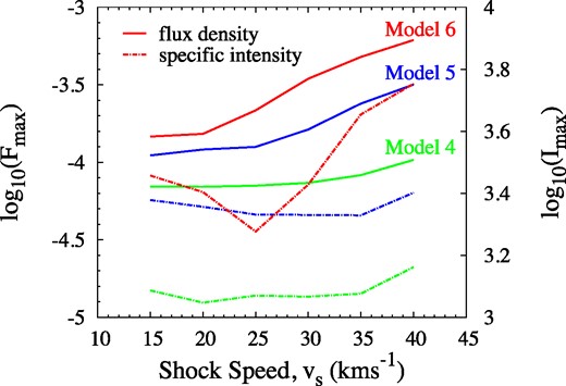
Flux density in the brightest spectral channel (left-hand y-axis and solid lines) and specific intensity in the brightest pixel (right-hand y-axis and chained lines) as a function of shock speed for the C-type shock models, Models 4–6. There is one pair of lines for each model. Colour codes are: green, Model 4, |$n(\rm {H_2})=5\times 10^7$| cm−3; blue, Model 5, |$n(\rm {H_2})=10^8$| cm−3, and red, Model 6, |$n(\rm {H_2})=2\times 10^8$| cm−3. Plotted flux density and intensity values are the highest found in the model, regardless of epoch, as in Fig. 8.
In all cases, the maximum flux density and maximum specific intensity achieved follow qualitatively similar functional forms. As expected, these are approximately exponential in the unsaturated regime, and linear in the saturated regime. Where the physical conditions in the post-shock gas are sufficient to cause collisional quenching, maser output begins to decline. The dividing line between the exponential and linear regimes is not clearly predictable on the basis of the pre-shock cloud alone, being close to τM = 6 for the curves corresponding to Models 1–3, but at only 2–3 for Model 0. The continued rise in the curves for Model 0 suggests a less complete saturation in this case. In Models 0 and 1, where the compression factor in number density is 9, all curves peak at the final epoch, so the points plotted on the black and green curves in Fig. 8 correspond to 100 per cent compression of the cloud. However, for Model 2 (compression factor 16) both flux density and specific intensity reach their maximum values before the cloud is fully compressed. Therefore, the points plotted on the blue curve correspond to shocked fractions of 75 per cent–80 per cent, dependent on τM, and specific intensities to 65 per cent–85 per cent. Corresponding fractions for Model 3 (compression factor 25) are 80 per cent–95 per cent shocked for flux density points and 65 per cent–90 per cent for specific intensity. We note that whilst Model 2 achieves slightly higher output in both flux density and specific intensity compared to Model 1, the output of Model 3 is much lower, especially at higher τM. This is at least in part due to the earlier onset of quenching, but almost certainly also involves a viewpoint effect (see Section 4.6 below).
The Model 0 curves are stopped at a pre-shock maser depth of 5.0: it is not reasonable to continue to higher depth, as further points would almost certainly correspond to fractional H2O abundances beyond the likely maximum of approximately 4 × 10⁻⁴ (van Dishoeck et al. 2021). If the model is also considered for evolved stars, there is a little more leeway in this respect, with fractional abundances closer to 10−3 reported for W Hya (Barlow et al. 1996) and VY CMa (Royer, Decin & Wesson 2010). We note that the peak τM obtainable with a constant abundance of 3 × 10⁻⁵ is approximately 15 from the peak of Fig. 2. To attain larger values of τM requires an increased water fractional abundance in the post-shock gas. In Model 0, with a compression factor of 9 and pre-shock depth of τM = 5, a post-shock depth of 45 is achieved, or approximately three times the constant abundance limit from Fig. 2. It is reasonable to treat this as a linear multiplier of the fractional water abundance in the saturated regime, implying a post-shock fractional abundance of 9 × 10⁻⁵ with respect to H2. The Model 0 curves therefore represent something close to the limiting values achievable for a hydrodynamic shock in a 1 au cloud.
The C-type models, Models 4–6, have a negligibly small pre-shock maser depth, which follows from placing the pre-shock ortho-H2O number densities (3–12 cm−3) from Table 1 on the x-axis of Fig. 3, and reading off the corresponding depth from the y-axis for a curve with T = 672 K. These models also have only one post-shock depth value, since we consider negligible compression during the passage of the H2O abundance front. Therefore, we plot instead the flux density in the brightest spectral channel and the specific intensity in the brightest map pixel as a function of shock velocity in Fig. 9 for three values of the pre-shock density. Almost all the peak flux densities occur at the last time sample, when passage of the abundance front is complete. However, the specific intensities peak at a variety of earlier times, almost certainly indicating competitive action between rays at the onset of saturation. It is also apparent from Fig. 9, that while the flux density at any speed rises with number density from Models 4 to 6, the specific intensities do so only in a velocity-averaged sense, and the specific intensity, at least in Models 4 and 5, is not a strong function of speed.
Light curves, with the flux density and peak specific intensity on linear scales, are shown for Model 2 (hydrodynamic, compression factor of 16) in Fig. 10 for all 8 values of τM studied. All of the subfigures are plotted on the same time range of 1000 d. To approximate a decay for the flare, we have again plotted exponentials in symbols with a time constant given by equation (15). However, the time constant in Fig. 10 is reduced to 71 d to allow for increased density, by a factor of 9/16, in the post-shock gas, compared to the Model 0 light curve in Fig. 6 The first three panels of Fig. 10, corresponding to pre-shock depth multipliers of τM = 1.0, 2.0, and 3.0 produce flares that would probably not be observable at distances of several kpc.

A sequence of light curves, showing the effect of increasing the initial optical depth of the model. Depth multipliers, τ, in the unshocked cloud, a measure of density and saturation, are marked in each subfigure. The compression factor of the shock, 16, the shock speed, 6.14 km s−1, and the viewpoint of the observer (|$\theta = \pi /2$|, ϕ = 0) are the same in all cases; these figures correspond to Model 2 in Table 1.
The counterpart to Fig. 10 for the C-type models is Fig. 11, where we plot the light curves for a 35 km s−1 shock at three different number densities of H2. No decays are shown. The likely outcome, after passage of the H2O abundance front is complete, is a flat, or slowly rising, segment until the momentum-transfer time is reached, at which point a combination of rapid cooling and high density quenching of the inversion are likely to cause the light curve to decay rapidly. If rapid loss of inversion sets in when the temperature of neutral molecules falls below 400 K, then the distance over which decay occurs, from cooling alone, is of order 3 × 1013 cm from fig. 2 of Kaufman & Neufeld (1996), or a time of 99 d for a shock speed of 35 km s−1.

A powerful flare must be observable, but another criterion of merit is the variability index that measures how bright the flare is relative to the quiescent state. For these models, this generally means the flux density from the shocked cloud divided by that from the unshocked original. We show this for Models 0 to 3 in Fig. 12. All graphs in Fig. 12 show a peak, representing the ‘best’ flare in the sense of a flux-density ratio. However, for all four models, these peaks are at lower values of τM than those corresponding to strong saturation from Fig. 8. There is therefore generally a compromise to be found between maximizing the variability index or the absolute flux density. We note also that the Model 0 variability indices can reach several million, whilst the more realistic models have variability indices that peak at values below 8000. The C-type models have an extremely small optical depth of H2O in the unshocked gas, and therefore an extremely large variability index.
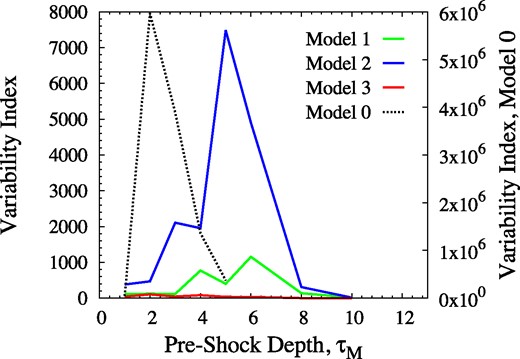
Variability indices in flux density as a function of pre-shock model depth for Model 0 and the sequence of Models 1–3 with line styles as shown. The left-hand y-axis is for the sequence of models, and the right-hand y-axis for Model 0 only.
4.6 Effect of viewpoint
Initially, we consider what happens when the observer’s viewpoint is moved to a selection of positions instead of the view close to parallel with the shock front, shown in Fig. 1. Before shock impact, the cloud approximates to a uniform sphere. A large sample of equidistant viewpoints leads to a calculation of the visibility solid angle, |$\overline{\Omega }_{\rm V}$|, of the source: the solid angle of sky that receives half the flux density of the source. The visibility solid angle should not be confused with the intrinsic beaming pattern that will be considered later. For example, a perfectly spherical maser cloud appears the same to all equidistant observers, and so has |$\overline{\Omega }_{\rm V}=2\pi$| sr. The same spherical maser, if highly amplified, might have a very small intrinsic beam solid angle |$\ll 2\pi$| sr, which would make the source appear much smaller than the physical cloud. For a measurement of |$\overline{\Omega }_{\rm V}$|, we choose the 100 per cent shocked cloud from Model 0 with a pre-shock model depth of τM = 5. The result of 1000 formal solutions in random directions in this case results in a visibility solid angle of |$\overline{\Omega }_{\rm V} = 0.452 \pm 0.013$| sr, for the brightest frequency channel, where the uncertainty is taken to be the solid angle corresponding to one solution, or 1/1000 of the sky in this example. This uncertainty estimate follows from the fact that a non-integer number of viewpoints contributes half the flux density, but we take |$\overline{\Omega }_{\rm V}$| from the nearest integer number. The |$\overline{\Omega }_{\rm V}$| parameter is useful in estimating the actual number of maser clouds that may exist in a source. Since the probability of observing a cloud at >0.5 of its maximum flux density is |$\overline{\Omega }_{\rm V}/(4\pi)$|, then a randomly placed observer might expect to see one bright cloud in every |$4\pi /\overline{\Omega }_{\rm V}$|.
We also show sample spectra derived from Model 0 at a compressed fraction of f = 0.75 in Fig. 13 to show the development of the total spread and the flux density as the viewing position is moved from zero (where the domain z-axis and the shock front are pointing directly towards the observer) through a number of different polar angles, as marked in degrees, up to 180°, where the observer views the cloud from behind the shock front. A logarithmic scale is used in Fig. 13 to make the spectra viewed significantly away from the 90° position visible. Note that channel number rises with frequency, so the dominant blueshifted peak from the shocked portion of the cloud appears to the right of the figure for a viewing angle of zero degrees, whilst a very similar redshifted peak (to the left) appears at 180°. The zero of the frequency axis corresponds to the unshocked portion of the cloud.
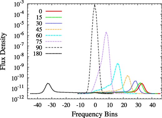
Logarithmic spectra from the Model 0 cloud at the polar viewing angles, θ, shown (in degrees). The frequency bin number rises with frequency (not velocity). The flux density represents a sum over all rays (pixels). Each ray has a specific intensity scaled to the saturation intensity, and the observer is at a standard distance of 1000 domain units.
Sample spectra for Model 5 with vs = 35 km s−1, as a representative C-type model, are shown in Fig. 14 for comparison with Fig. 13. It is immediately apparent that, without the deformation of the cloud, the bias of high flux density to viewpoints parallel to the shock front is much less pronounced, making the C-type model significantly less sensitive to the observer’s viewpoint. In this type of model, a bias to higher flux density when viewed parallel to the shock front is due only to the velocity gradient along the z-axis. The result of the visibility solid angle calculation in this case is |$\overline{\Omega }_{\rm V} = 3.091 \pm 0.013$| sr. This much larger value, when compared to the hydrodynamic case of Model 0 above, confirms numerically the reduced sensitivity to viewpoint of the C-type models that is suggested by Fig. 14: a randomly placed observer would be 6.8 times more likely to see the flare from Model 5 than from Model 0.
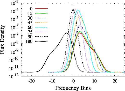
As Fig. 13, but for the C-type model with a shock speed of 35 km s−1 from Model 5.
Returning to the situation of a fixed observer, another great advantage of a 3D model is that it is possible to compute the intrinsic beaming solid angle of the maser at any point on the surface of the cloud. Operationally, we choose a target point on the external surface of the domain, along the direct line of sight to the observer from the domain origin. The maser beaming pattern at this target point can then be computed by calculating the specific intensities of a large number of rays that converge on the target from points on a spherical background. If each ray has a very similar solid angle of sky associated with it at the target, then the beaming angle at that point may be straightforwardly calculated by ordering the output specific intensities in brightness, and counting the number N that generate half the observer’s flux density. The half-flux density beaming angle, ΩM, is then |$\sum _{i=1}^N \delta \Omega _i$| if ray i has an associated beaming solid angle δΩi at the target. If we also approximate the beaming pattern as an ellipse of solid angle |$\Omega _{\rm M} = \pi \delta \theta _{\rm M} \delta \phi _{\rm M}$|, where δθM (δϕM) are the intrinsic polar (azimuthal) beaming angles, then the calculation of ΩM, and one of the directed beaming angles provides a complete solution of the beaming-angle problem for one target point. For example, an accurate value of ΩM = (8.33 ± 0.60) × 10−5 sr was computed by taking the mean value of 100 similar target points observed parallel to the shock front for the case of the 100 per cent shocked Model 0 with an initial depth multiplier of 3.0. Beam solid angles smaller than this have been suggested previously (Nedoluha & Watson 1991).
There is a practical problem in the computation of the beaming angles: the number of rays must be sufficient to resolve the (very small) beaming solid angle. We increased the order of a healpix partition of the sphere (Górski et al. 2005), measuring the beaming solid angle in each case, and found that the beaming solid angle became significantly larger than the solid angle associated with an individual ray at order 9, which partitions the sphere into 3 145 728 panels of equal area, each with one ray originating from its centre. Beaming angle computations were therefore carried out at order 9, with occasional tests at order 10 (12 582 912 rays). We note that our healpix algorithm was coded from formulae in the published work cited above, and did not use any software from the healpix website or project.
We now compare the observer’s view of the source for a hydrodynamic model in the polar and azimuthal directions, where the shocked part of the cloud is highly compressed. The effective geometry of the compressed cloud, or compressed part of a cloud, is that of a short cylinder, and in the polar direction the observer looks along the short edge of the cylinder, perpendicular to the shock front (see Fig. 1). In this simple representation, there is no curvature of the source in this direction, and it therefore approximates to the ‘screen’ type maser in fig. 4.1a of Gray (2012). Also, although the polar beaming angle will be small in the sense that its sine and tangent approximate to the angle itself, it will still be much larger than the typical angular extent of the source, so that we are in the ‘size-limited’ case, resulting in the flux density equation (4.48) of Gray (2012), which is independent of the intrinsic beaming angle. This is why a model computation of δθM is particularly important: it is very difficult to obtain from observations, but may be estimated from a sequence of VLBI channel images that have a position–velocity gradient, allowing the cloud size to be estimated from the range of spot positions (Richards et al. 2012). With a simultaneous measurement of the angular FWHM (full width at half-maximum) of each spot, the beaming angle can be calculated. However, this method needs high sensitivity and assumes an at least approximately spherical cloud surface. Any brightness variation in the polar direction in images, such as those in Fig. 5, is only due to intrinsic brightness variations as a function of z-position along the cylinder edge in Fig. 1, and this surface is not curved in this direction.
The source surface in the azimuthal direction is curved, following a circular path, parallel to the shock front, and in or out of the plane of the page in Fig. 1. Unlike the polar direction, we now expect the central intensity of the beaming pattern to vary very little as the circular path is followed, so that variations in observed intensity for a fixed observer, with sin θ ≃ 1 and a particular azimuthal angle, ϕ, depend upon both the intrinsic azimuthal beaming angle, δϕM and the curvature of the source surface. The situation in the azimuthal direction is now rather like fig. 4.1b in Gray (2012), with the flux density given by a solution of equation (4.52). With symbols, the angular radius of the source in this case can be written,
where αmax is the measured angular radius of the source at FWHM, R is the radius of the short cylinder that represents the shocked region, and d is the distance of the source from the observer. Note that in this case, δϕM can be recovered from an interferometric observation of αmax, provided that R and d are known independently, and that the angular resolution of the observation is sufficient to determine αmax. From the modeller’s perspective, the angular resolution provided by the set of rays in Fig. 5 is too coarse to resolve the azimuthal beaming angle, so we compute it using the healpix method introduced above, together with measurements of the asymmetry of the beaming pattern. The beaming pattern is typically extended in the azimuthal direction, and an example is shown in Fig. 15, noting that this diagram shows the true aspect ratio of the beaming pattern, which is 5.17 for Model 0 and initial τM = 3.0. Using the ellipse approximation for the beaming pattern, and the computed value of 8.33 × 10⁻⁵ sr for ΩM, we derive polar and azimuthal beaming angles of δθM = 2.26 × 10⁻³ rad (0.129 degrees) and δϕM = 1.17 × 10⁻² rad (0.667 degrees) for the 100 per cent compressed cloud from Model 0 with τM = 3.0.
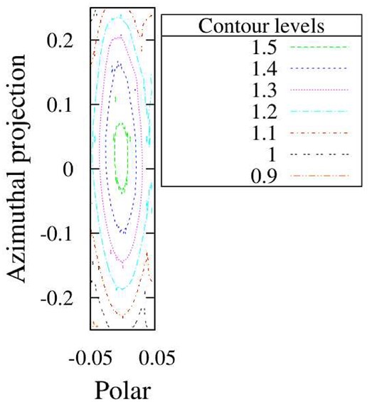
Contours of the intrinsic beaming pattern for Model 0 and initial depth multiplier 3.0. levels are in log10 of (the specific intensity in multiples of the saturation intensity). Each ray has an angular offset from the direction of the brightest, and the x- and y-axes are the respective projections of this offset on the polar and azimuthal directions, measured from the centre of the beaming pattern (the brightest ray). The x- and y-axis scales are equal to demonstrate the azimuthal extension of the beaming pattern. A line towards the observer points out of the page.
The ratio δϕM/δθM appears remarkably constant over the range of depths shown in τM. For Model 0, this ratio ranges from 5.2 to 7.6 between depths of τM = 0.2–4.5 with no clear trend to increase or decrease. Measurements are rather inconsistent because the brightness ranges that can be contoured vary so much over the range of depths used. It is probably significant, however, that δϕM/δθM is larger for the submodels of Model 1, ranging from 7.8 to 9.4, again with no clear trend, over the initial depth range of 1.0–12.5. This difference must arise from some factor other than the compression factor, which is the same in Models 0 and 1.
Having considered some particular examples, we plot in Fig. 16 the beaming solid angle (left-hand y-axis and black lines) and the polar intrinsic beaming angles (right-hand y-axis and red lines), at a similar range of depths, for Model 0, and for Model 1, as in the figures from Section 4.5. In both black curves, the beaming solid angle falls with rising τM. There is no clear residual level reached for Model 0, but the curve for Model 1 flattens at a level of approximately 1.3 × 10⁻⁵ sr. The polar beaming angle does appear to re-broaden at the last point (τM = 5.0), for Model 0, due to an exceptionally small value of 4.1 in δϕM/δθM. The minimum is 1.12 × 10⁻³ rad (0.064 degrees), at τM = 4.5, before the apparent re-broadening under strong saturation. The red dotted curve, representing δθM for Model 1, follows the solid angle in apparently flattening out at the highest depths used. In this case, values of δϕM/δθM remain typical for the last pair of points, with δθM flattening at a value of approximately 7 × 10⁻⁴ rad (0.04 degrees). Azimuthal beaming angles can be recovered from all depth in Fig. 16 from the polar angles, beaming solid angles, and the ellipse assumption for the beaming pattern.
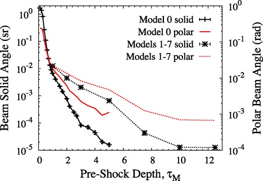
Beaming solid angles (black lines with symbols) and beaming angles in the polar direction (perpendicular to the shock front; red lines without symbols) as a function of the model depth in the unshocked cloud. Solid lines are for Model 0 and dashed lines for Model 1. All these models have a compression factor of 9. Error bars at points on the solid angle lines show the standard error, based on the mean of 30 evenly spaced azimuthal viewing positions.
In the case of MHD models, there is again no set of pre-shock τM values to use as the x axis of a graph similar to Fig. 16. However, we computed a one-off value of the beaming solid angle, and the polar intrinsic beaming angle, for Model 5, v = 35 km s−1. The respective values were ΩM = 1.43 × 10⁻⁴ sr and δϕM = 8.33 × 10⁻³ rad (0.48 degrees). These beaming angles are substantially larger than those found for the hydrodynamic models under similar levels of saturation. We also found that the beaming pattern is less extended in the azimuthal direction in the MHD models with a ratio of δϕM/δθM = 1.54. The beaming pattern for Model 5, v = 35 km s−1 is shown in Fig. 17.
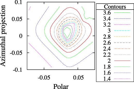
As for Fig. 15, but for the C-type model, Model 5 with a shock speed of 35 km s−1.
It is possibly also useful to consider the variation of beaming angles with the shock fraction, f, in the cloud, and an example is plotted in Fig. 18. An assumption made for this plot is that the beaming angle is unaffected by the radiation from the unshocked part of the cloud. This is a reasonable assumption once a significant fraction of the cloud is compressed, since the radiation from the unshocked part of the cloud is usually much weaker. The data are from Model 1, and the submodel has a pre-shock depth of τM = 7.5. There are almost certainly larger uncertainties arising from the exact position of the line of sight and the discretization of the domain than the error bars shown in Fig. 18, which correspond only to the standard error on a mean of 30 azimuthal angles, and this is particularly true for low values of f, where the fraction of nodes in the compressed region is small. There is a trend of falling ΩM until the compressed fraction reaches 0.4–0.6, with little change thereafter, though there is possibly a small, but significant, broadening at f = 0.9–1.0.
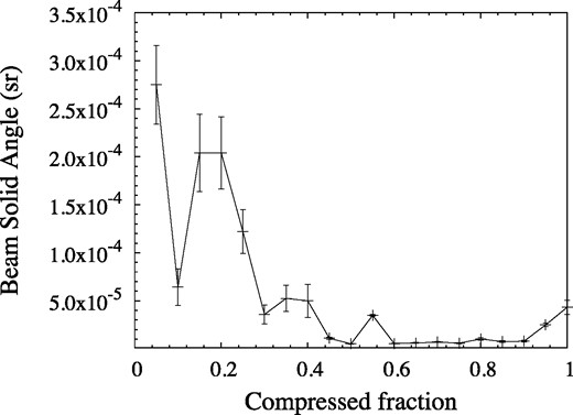
Variation of ΩM with compressed fraction, f, for Model 1 (pre-shock maser depth = 7.5). Error bars are shown for the standard error on the mean of 30 azimuthal observation angles.
4.7 Effect of shock speed
In this section, it is straightforward to study a full set of C-type models, since these have submodels identified by shock speed, varying from 15 to 40 km s−1, and each model has a fixed density. In the case of the hydrodynamic models, Models 1–3, there is one velocity only for each complete model, and we choose submodels that have a depth parameter that gives close to maximum output (plotted in Fig. 8): we use τM = 8.0 for Models 1 and 2, but τM = 6.0 for Model 3, so as not to be too greatly affected by quenching in Model 3. With these settings, post-shock conditions in all three models are close to the peak of Fig. 2. For each shock speed, we plot a light curve. Owing to the considerable range of shock speeds, we do not plot the x-axis in time, but in fraction of the cloud swept. This parameter exceeds 1.0 for the C-type models to allow for the passage of a transition zone, in which the H2O abundance rises from its pre-shock value to its full post-shock value (4 × 10⁻⁴ with respect to H2 in Models 4–6) after passage of the abundance front.
We plot light curves for the nine shock speeds in Fig. 19. For the C-type shocks, the general trend is for the flux density achieved at the peak of the flare to rise with shock velocity, and therefore with the velocity shift present in the cloud. However, the final flux densities achieved differ by only a factor of ∼ 3 between velocities of 15 and 40 km s−1. As expected, the rise towards the peak is progressively more delayed as the shock speed is reduced, and the transition zone becomes wider. There appears to be a significant secondary effect in that the C-type light curves are smoother than those of the hydrodynamic models. The hydrodynamic models also tend to have light curves that peak at a lower shocked fraction than 1.0 at the higher shock speeds, so that there is already a significant decay in flux density of Models 2 and 3 by the time the shock passage through the cloud is complete. The shocked fractions yielding the highest flux density in Models 2 and 3 are typically 80 per cent–90 per cent (see Section 4.5). The optimum amount of overall compression for a bright flare appears to be somewhere between 16 (Model 2) and 25 (Model 3).
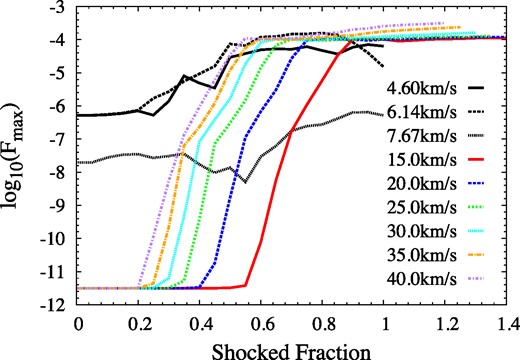
Light curves for nine different shock speeds, as marked in the key. Black lines correspond to hydrodynamic models (Models 1–3 in order of increasing speed) and other colours, or lines beginning at a y-value smaller than -11, to the C-type shocks of all speeds from Model 5. The x-axis is the fraction of the z-axis extent of the cloud traversed by the shock (or the H2O abundance front in the C-type cases) and the y-axis is the base-10 logarithm of the flux density.
As a complement to Fig. 19, we plot light curves for Model 5 at all shock speeds on a linear scale in Fig. 20, with a standard time range of 400 d, so that the shortening of the shock duration with rising shock speed can be appreciated. In these light curves, we have not followed the model evolution through the decays which would be expected to be of duration similar to the momentum-transfer time, due to a combination of compression quenching and cooling of the cloud.
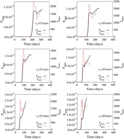
A sequence of flare light curves, showing the effect of increasing shock speed, as marked for each subfigure. All these speeds conform to the labelling of submodels from Table 1. The H2 number density in cloud is 108 cm−3 in all cases, and the viewpoint (|$\theta =\pi /2,\phi =0.0$|) is as in Fig. 10. All subfigures are shown over the same time range of 400 d for comparison.
5 DISCUSSION
The question to be discussed is, ‘how good is a shock mechanism for generating flares?’. The answer is ‘very good’, provided that there is no requirement of periodicity, in the sense of single clouds, rather than whole source regions, and that the transition concerned has a pumping scheme that is dominated by collisions. Variability indices can reach the order of millions for shocks that approximate to ideal hydrodynamic, isothermal types, but hundreds to thousands are probably more typical given the work presented in Section 4.5. Rise time-scales of order 30 d are achievable for au-radius clouds, but the overall flare, particularly in the case of C-type shocks, with a long momentum-transfer time, can take an order of magnitude longer, and the behaviour after the shock passage is complete, including the time for relaxation, is not addressed in any detail by the current models. We consider our results for achievable flux density and variability index to be somewhat conservative, since the parameter Γ in equation (16) has been considered a constant, but is likely to increase somewhat in the post-shock gas because it contains density-dependent collision rates. Any increase in Γ raises the saturation intensity, allowing higher intensities to develop before the onset of saturation.
Much of the work reported above has concentrated on au-scale clouds, and a single one of these, at kpc distance, can produce a flare of order 100 Jy under the best conditions of viewing angle and shock properties (peak flux density of Model 0 from Fig. 8 and equation 18). The more realistic models are somewhat less effective, largely because of the quenching effect on the maser inversion of very high densities. An important point that enhances the potential of shocked clouds to explain very large flares is the result that the bright part of a shocked cloud appears substantially smaller than its pre-shock counterpart and, given the limited dynamic range of telescopes, a measured, single-channel, spot size of order 1 au may imply that the original cloud had a radius of 25–40 au. With this sort of logic, an observed 1 au feature could flare to some thousands of Jy at kpc distances. However, there are limits to this consideration of ‘invisible’ pre-shock material imposed by the need to keep time-scales short enough. In terms of sensitivity to the viewing angle, C-type shocks are considerably more visible because the cloud is not significantly compressed during the rise time of the flare, and there is consequently less restriction to lines of sight close to parallel with the shock front.
Flares of the highest flux density, for a given cloud size, require a density enhancement in the post-shock gas that places the number density of the maser species close to the quenching density (for o-H2O parameters, close to the peak of one of the curves in Fig. 2, or Fig. 3). Pre-shock conditions that include a number density well to the low side of the quenching density, and therefore to a high shock speed (in hydrodynamic models) with a pre-shocked cloud of low, probably unsaturated, maser depth are also pre-requisites for a very high variability index. This view is supported by the observation that almost all strongly saturated nodes (those with remaining inversion <0.9) are found in the shocked part of the domain (see Fig. 4). This saturation distribution follows from the fact that only the shocked gas can contain rays that pass diametrically through material that is all at the high, post-shock density. C-type models have no difficulty in this respect, since the pre-shock material has a very low value of τM (or inversion), and the variability index is consequently very high. It is quite possible that an additional mechanism is required to explain the very brightest H2O masers flares, for example line-of-sight overlap between clouds for the 140 kJy outburst in W51 (Volvach, Volvach & Larionov 2023).
Models 4–6, based on MHD shocks, lead to flares with rise times of shorter duration than pure hydrodynamic systems (see Fig. 20). This is partly due to the fairly obvious point that an MHD shock needs to be faster than a hydrodynamic type to achieve the same ultimate compression factor. However, this is offset to some extent by the delay introduced by a transition zone in which the abundance of H2O rises towards its final value. A much longer delay in decay, that is necessary for the momentum coupling of the ionic and neutral fluids, may make the overall flare from a C-type shock at least as long as that from a significantly slower hydrodynamic type with prompt compression. Decay times in the C-type case are difficult to predict with the current version of the code, and may include contributions from cooling, compression beyond the quenching limit for the inversion and dispersion of the final, compressed cloud on a time-scale based on the post-shock Alfvén speed, which is considerably larger than the isothermal sound speed for Models 0–3. The fastest reasonable C-shock speeds can probably produce a flare that is complete within ∼800 d for an original cloud of radius 1 au, at least an order of magnitude longer than the rapid initial rise times in Fig. 20. It is apparent from Figs 10 and 11 that the rise time of flares is rather insensitive to the optical depth of the medium. However, increasing saturation smooths the light curve during the brightest part of the flare, where it has become comparable to the peak value after a rise time of order a few × 10 d. Overall, the form of the light curve from a flare is an important observational diagnostic.
This work has concentrated on deriving the parameters of maser flares that can be generated by the impact of a shock wave on an individual cloud or condensation. It is perhaps interesting to speculate on how many such objects might be able to contribute to a flare in a real source. An estimate of 100 ‘hotspots’ for H2O masers in a typical star-forming region source was made by Strelnitski (2007), some or all of which might take part in a maser flare. Such a number makes it quite easy to achieve flux densities of thousands of Jy from groups of au-scale clouds at kpc distances. Groups of maser, or potential maser, clouds also allow us to consider a shock mechanism as a source of periodic or quasi-periodic maser flares: if a periodic event generates a sequence of shock waves, then even if shock passage destroys individual clouds, a new group may be excited and compressed by the next shock, leading to periodicity in a statistical sense.
Beaming solid angles of the size derived in Section 4.6 certainly make it possible to achieve the very high brightness temperatures discussed in Section 4.4. Also, measured azimuthal beaming angles are potentially useful for determining the saturation state of a shock-driven maser flare, particularly if there is an independent measurement of the shock speed, which likely controls the asymmetry of the beaming pattern. Given that the models discussed in Section 4.6 always show a significant asymmetry, then for the same beaming solid angle, a shocked cloud will always exhibit an azimuthal (polar) beaming angle that is larger (smaller) than the beaming angle derived for a spherical cloud. It is not clear how this beam structure, based on a model approximating to the ‘short cylinder’ shocked slab in Fig. 1, relates to the long filamentary cylinder approximations (length to diameter ratio 5–50) described in Elitzur et al. (1989). Perhaps in the most general terms we can consider the filament diameter to correspond to the thickness of the compressed layer in our hydrodynamic models, and the filament length to the original cloud diameter. This then leads to aspect ratios (length/diameter) of 4–16. These figures are consistent with the lower part of the range in Elitzur et al. (1989). The upper range is perhaps not accessible because of our lower shock speeds.
In terms of the definitions used in Richards et al. (2011), we expect the shock-generated masers from our hydrodynamic models to be ‘matter bounded’ (Elitzur et al. 1992) in the polar direction, so that we should see something close to the full thickness of the compressed region of the cloud. We expect amplification bounded emission in the azimuthal direction because of the curvature of the surface in this direction. C-type models are closer to amplification bounded in both directions, but still have a substantial brightness bias to polar angles near |$\pi /2$|. Beaming-angle asymmetry yields a relatively large beaming angle in the azimuthal direction, so that the predicted extension in this direction is larger than would be expected for a circular beaming pattern. We therefore expect images of shocked clouds to be a better approximation to their true size when measured along the minor axis, that is perpendicular to the shock front, compared with spherical clouds of constant velocity, where the maser image at half flux density is significantly smaller than the actual cloud radius (Elitzur et al. 1992; Gray et al. 2018). This expectation appears to be substantially borne out in the images in Fig. 5. As a further check, Richards et al. (2011) predict that the observed size of a shock generated, matter-bounded, maser should be rather insensitive to the frequency channel at which the observation is made, but that an amplification-bounded maser should appear much larger in the line wings, for example 69 times larger comparing the large and small box areas in their Fig. 9 (lower panel). When we plot object area, at the half flux-density level, relative to the value at line centre in Fig. 21, we see a broad minimum, covering about 2.3 Doppler widths. We suggest this region is dominated by the brightest, matter-bounded emission, before the very faint azimuthally extended emission, that is amplification bounded, produces much larger areas in the extreme line wings. However, this increase in area would not be detectable to a telescope with a dynamic range of ≲ 106, as can be seen from the overplotted spectrum in Fig. 21.
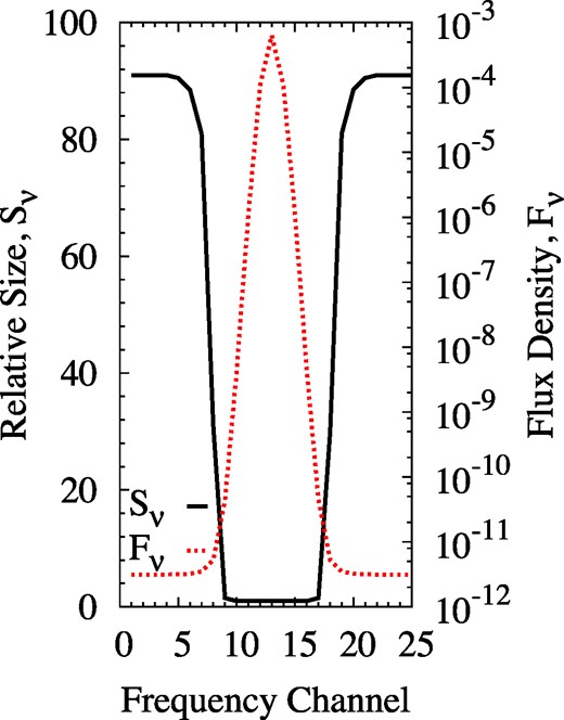
Apparent area of the maser cloud at the half flux-density level as a function of frequency (black solid line), and the logarithmic spectrum (red dotted line) for comparison of widths. The area scale sets the minimum value to 1.0, and the line centre of this figure corresponds to the final panel of Fig. 5: Model 0, initial depth 3.0 and compressed fraction 1.0. The 25 frequency channels shown cover 7 Doppler widths. The viewpoint is |$(\theta ,\phi) = (\pi /2,0.0)$|.
5.1 Relevance to accretion sources
It is instructive to discuss how our models of shock-excited maser flares from individual au-scale clouds fits into the broader picture of a global source geometry, particularly a source of the classic type combining an accretion disc and bipolar outflow. A source of this type that has been observed in particular detail is IRAS21078 + 5211, in which 22-GHz H2O masers exhibit outflow-oriented proper-motions, and have been analysed as having a disc-wind origin (Moscadelli et al. 2022). Scatter in vLSR of several km s−1 is said to be inconsistent with much smaller positional scatter of VLBI maser features, and therefore evidence for excitation by weak C-type shocks travelling through the maser clouds. In this source, we identify our maser clouds with the observational radio knots in Moscadelli et al. (2022): these are clearly resolved into small clusters of distinct objects at the 0.7 mas resolution, giving a linear scale of 1.14 au at 1630 pc that is consistent with our model cloud scale. Physically, the maser clouds would be regions of enhanced density in the MHD disc wind resulting from variations in the physical conditions near the disc surface. A variability time-scale of order 1 month (Moscadelli et al. 2022; Krasnov et al. 2018) related to individual spectral features is consistent with, for example, our Model 4 (top panel, Fig. 11) in which more than half the maximum flux density, and the brightest specific intensity are achieved within 20 d of flare onset. The shock speed in our figure is 35 km s−1, though two-thirds of this speed, 23 km s−1, would still yield a rise time of 30 d. which is also consistent with month-scale variability. These modelled speeds are rather difficult to match to any precise values from observations: Krasnov et al. (2018) suggest ∼15 km s−1, whilst fitted flow velocities, of which the shock velocity is presumably a significant fraction, in Table 2 of Moscadelli et al. (2022) range from 9 to 85 km s−1.
The introduction to this work refers to a couple of accretion-burst sources. It is not obvious that a shock-based variability mechanism should apply in such objects, since the main result of an accretion event is a burst of radiation, often powerful in the IR, that favours radiatively pumped maser transitions. A case in point is the MM1 source in the massive star-forming region G358.93 − 0.03, where the progress of the ‘heat wave’, or radiation burst, was tracked across the nearly face-on accretion disc via its effect on 6.7-GHz CH3OH masers (Burns et al. 2023). A clear link between spiral sub-structures in the accretion disc of MM1 and accretion bursts has been demonstrated by Chen et al. (2020). Several radiatively pumped maser species, particularly three newly discovered transitions, traced the spiral substructure in the disc, and flared following the IR radiation enhancement from the accretion burst. However, the 22-GHz H2O masers in this source are more mysterious, because of a lack of interferometer data during the H2O flare, which was delayed by ∼100 d with respect to 6.7-GHz CH3OH. There are two e-VLA images of G358.93 − 0.03 before and after the H2O maser flare, showing drastic change in the source structure (Bayandina et al. 2022). Whilst the 22-GHz masers in MM1 itself are significantly altered, spectrally and spatially, the distribution is broadly aligned with the outflow in the before and after images. However, maser clusters in the more distant sources MM2, MM4, and MM5, present in the ‘before’ image became undetectable, and a new source appears in the ‘after’ image between MM4 and MM5, though probably associated with the latter. Bayandina et al. (2022) specluate that the H2O maser flare is associated with this new source, noting that the vacuum light travel time from MM1 to the new source (in the sky plane) of 78 d is comparable to the 100 d delay in the maser flares. If this association is correct, we offer two possibilities for the generation of the new H2O maser cluster. The first is that the radiation from the accretion event in MM1 has an SED that is IR-dominated, and very similar to those in Stecklum et al. (2021). This radiation impinges on gas containing very dense (∼1010 H2 cm−3) and cold (<50 K) water molecules. Under these conditions, a radiative pumping scheme can operate for the 22-GHz transition (Gray et al. 2022). This possibility is attractive in that the IR burst is destructive for the existing masers in hotter, more rarefied conditions, but can explain the rapid rise of the flare (over 20–30 d, Bayandina et al. 2022) in a previously maser-free site. The second possibility is that the dust shrouding of the young stellar object in MM1 is patchy, allowing radiation approximating to its raw SED to escape along certain lines of sight. Assuming most radiation with λ < 111 nm, is lost in dissociating or ionizing hydrogen, there is still a band 145–111 nm that can heat gas efficiently due to photoelectric emission from grains. The nine best burst models in Stecklum et al. (2021, their table A6) have a mean stellar temperature, T*, of 22 570 K and mean radius of 10.31 R⊙. From formulae in section 30.2 of Draine (2011) such photoelectric emission deposits energy at an approximate rate of |$9.28\times 10^{-27} n_{\rm H} (n_\gamma /3\times 10^{-3} \rm {cm^{-3}})$| erg cm−3 s−1, where nγ is the number density of the UV photons and nH is the number density of H-nuclei. The radiation field, at T*, diluted to a distance of |$13\, 500$| au, has nγ ≃ 270 cm−3 of photons in the 145–111 nm band, so for a number density nH = 2 × 108 cm−3, typical of the pre-shock gas in the C-type models used in this work, the photoelectric heating rate is 1.64 × 10⁻¹⁴ J m−3 s−1. An increase, ΔT, in the gas thermal energy due to this heating rate, Γpe, follows |$\Delta T= 2\Gamma _{\rm pe} t/(3 k_{\rm B} n_{\rm H_2})$| after t seconds. From this formula, a temperature increase of 800 K requires only a little over 100 s. There remains the question of how quickly this energy can be transferred from the photoelectrons to the H2 gas. For electron kinetic energies of a few eV, the elastic collision cross-section for collisions with H2 are typically >10−19 m2 (Yoon et al. 2008), so the mean-free time for the electrons is |$1.7\times 10^5\,(E_{\rm eV}^{1/2})^{-1}$| s. Energy can therefore be transferred from the radiation field to the H2 gas within a few days. The rate of energy deposition will, of course, fall as the radiation progresses into the gas. We use an extinction cross section due to dust of 8.16 × 10⁻²⁶ m2 at 100 nm to calculate an optical depth at this wavelength of τ1000 = 2.441Lau, so the energy is mostly deposited in a layer of astronomical-unit scale, linking ultraviolet extinction by dust to the scale of model clouds studied in this work. Since the time required for heating is much less than the sound crossing time of the heated region, the heated gas will become hot and overpressured with respect to its surroundings. Under these conditions it is very likely that shock expansion will follow into cooler gas further from the radiation source. In this way, an initial radiative event caused by accretion can ultimately drive a collision-based pumping scheme after a delay little longer than the light travel time to the new maser zone.
6 CONCLUSIONS
Shock-wave modification of gaseous clouds of scale a few au to a few tens of au provides a mechanism that can explain maser flares with the largest observed brightness temperatures (≳ 1017 K). The mechanism is limited to transitions with a mainly collisional pumping mechanism, and the output is highly directional, dominated by directions parallel to the shock front, but this effect is less pronounced for C-type shocks. Magnetically dominated (C-type) shocks can generate masers with similar flux densities to the ideal hydrodynamic variety, and the magnetic types typically produce flares with an extremely large variability index, since these models have a minimal inversion in the 22-GHz transition of the maser species (ortho-H2O) in the pre-shock fluid. C-type shocks also produce flares of shorter duration, particular during the rise to peak, because faster shocks are required to achieve the same (ultimate) compression. Density of the maser species in the post-shock gas is important, but only in the sense that it needs to be in a ‘sensible’ range that is sufficient to achieve saturation, but low enough to avoid quenching the pump. Maser beaming pattens show a strong asymmetry, being considerably more extended parallel to the shock front. We find consistency with earlier work that suggests that the observed image, perpendicular to the shock front, in a shock-generated maser is much closer to the true size of the supporting cloud than in the quiescent spherical case.
ACKNOWLEDGEMENTS
MDG and SE acknowledge funding from the UK Science and Technology Facilities Council (STFC) as part of the consolidated grant ST/P000649/1 to the Jodrell Bank Centre for Astrophysics at the University of Manchester. MDG acknowledges financial support from the National Astronomical Research Institute of Thailand (NARIT) whilst on sabbatical at their HQ in Chiang Mai, Thailand. This work was performed, in part, using the DiRAC Data Intensive service at Leicester, operated by the University of Leicester IT Services, which forms part of the STFC DiRAC HPC Facility (www.dirac.ac.uk). The equipment was funded by BEIS capital funding via STFC capital grants ST/K000373/1 and ST/R002363/1 and STFC DiRAC Operations grant ST/R001014/1. DiRAC is part of the National e-Infrastructure. Data used in this work were generated under DiRAC award dp124. The authors would also like to thank the management of the Chalawan supercomputer at NARIT.
DATA AVAILABILITY
The data underlying this article will be shared on reasonable request to the corresponding author.
Footnotes
Directly proportional to inversions in column 5.
Directly proportional to inversions in column 6.
References
APPENDIX A: VARIABLE VELOCITY DEVELOPMENT
With reference to equation (2), we define here the symbols used. The velocity width parameter is |$W(\tau) = \sqrt{2 k_{\rm B} T_{\rm K}(\tau) / m_X}$|, and its domain average by node is |$\bar{W}$|, where kB is Boltzmann’s constant, TK is the kinetic temperature, and mX is the molecular mass of species X. Scaled distance along a ray, propagating in direction |$\hat{\boldsymbol {n}}$|, is represented by the optical depth τ. The parameter η(τ) is |$\bar{W}/W(\tau)$|, and dimensionless frequency and velocity are respectively denoted by |$\bar{\nu }$| and |$\boldsymbol {u}$|. The background dimensionless specific intensities, iBG(Ω), are also multiples of the saturation intensity, and here we allow for the possibility that the background level may vary with direction (Ω) on the sky surrounding the domain.
As in Papers 1–3, a nodal solution for the inversion is found through a saturation term that involves a frequency-and-angle averaged intensity that is itself eliminated in favour of an expression in terms of the inversions in nodes that border the ray paths converging on the node in question. In the earlier papers, it proved possible to perform the frequency averaging analytically, but this cannot be applied with variable velocity: although the analytical frequency integral can still be carried out, the resulting expression cannot be factored to restore multiple integrals (from the power-series expansion of an exponential) to the product of identical integrals, each in a single spatial variable. It is therefore not possible to reduce the expression to a single power series with one spatial integral as the argument. We therefore adopt the rather different strategy described here.
A formal frequency average of equation (2) over a Gaussian molecular response generates the averaged intensity,
where we have now assumed that η, the width parameter, is 1 everywhere, equivalent to assuming that the domain is isothermal. The frequency integral in equation (A1) is now modified by defining the new dimensionless frequency |$\varpi = \bar{\nu } - \hat{\boldsymbol {n}}_q \cdot \boldsymbol {u}(\boldsymbol {r})$|. This change of variable is applied to make the Gaussian in equation (A1) zero-centred, as convenient for numerical quadrature. With the further definition |$\Delta \boldsymbol {u}(\tau ^{\prime }) = \boldsymbol {u}(\boldsymbol {r}) - \boldsymbol {u}(\tau ^{\prime })$|, and specifying the intensity of a particular ray, q, equation (A1) becomes
The exponential in braces in equation (A2) contains a spatial integral that is discretized according to a finite-element scheme similar to that used in Papers 2 and 3. We first define
where the expression in equation (A3) shows the integral along ray q separated into the J(q) elemental contributions that appear between the entry point to the domain and arrival at a target node. The integral in equation (A3) is now over the path through a single element, j, with entry point τin, j, and the corresponding exit point τout, j. The expression for Yq is equivalent to the argument of the main exponential in equation (A2), so this can now be written in the much simpler form,
If the jth element has a shape function for its ith node of the form,
where x, y, and z are dimensionless coordinates within the element, and the quantities with the subscript i are shape-function coefficients, then fi can be parametrized in terms of a single variable 0 ≤ t ≤ 1, for example,
where (xin, yin, zin) are the coordinates of the entry point τin, j, and (Δx, Δy, Δx) are the coordinate differences between the exit and entry points. Summing terms that do not multiply t as Ai = ai + bixin + ciyin + dizin, and those that do, as Bi = biΔx + ciΔy + diΔz, the ith shape function becomes simply,
Any spatially variable quantity can then be found, in the interior of element j, by summing equation (A7), multiplied by nodal values of the quantity, over the nodes. For example, for some ray distance τin, j ≤ t ≤ τout, j, the dimensionless bulk velocity is approximated by
where |$\boldsymbol {u}_m$| is the velocity at the mth mode, and each element has M nodes. A similar expansion to equation (A8) is made for the unknown, δ′(t).
We now use equation (A8) and its analogue for δ′(t) to write Yq in terms of nodal values of quantities that vary across the domain. With the aid of the further definitions,
where |$\boldsymbol {u}_i$| is the velocity at the target node, and
Equation (A3) reduces to the form, with τj as the distance covered in passing through element j,
There are various ways of carrying out the integral in equation (A11): perhaps the most satisfactory is to extract a factor of |$\exp -[\alpha _{qj}^{(\varpi)}]^2$| from the integral, while defining new constants |$a = \beta _{qj}^2$| and |$b= \alpha _{qj}^{(\varpi)} \beta _{qj}$|, reducing equation (A11) to the form
that is tractable in terms of standard integrals. Of particular interest is the formula from Abramowitz & Stegun (1972), reproduced here as
where κ is a constant of integration. One integral is exactly of this form, and the other is reducible to this same integral through integration by parts. Results are in terms of exponentials and error functions, and the integrated form of equation (A12) is
where further new constants are |$\alpha _{qj} = \alpha _{qj}^{(\varpi)} - \varpi$|, γqj = αqj − βqj, and εqj = αqj + Ajμβqj/Bjμ. If the double sum over elements and local nodes in equation (A14) is replaced by a single sum over the global node numbers of those nodes that bound ray q, noting that such nodes may be members of more than one element in J(q), then we can pre-compute the coefficients, |$\Phi _{j,k}^{q,i}$|, where j is now the global node index. These coefficients include everything in equation (A14) except the nodal values of the inversion itself, |$\delta ^{\prime }_\mu$|. It is now possible to write equation (A14) in the simple form |$Y_q = \sum _{j=1}^{J(q)} \delta ^{\prime }_j \Phi _{j,k}^{q,i}$|. We substitute this expression for Yq in equation (A4), noting that Yq is a function of ϖ through the coefficients |$\Phi _{j,k}^{q,i}$|. We now replace the frequency integral with a Gauss–Hermite numerical quadrature with K abcissae, ϖk, and corresponding weights ζk, with k in the range 1 to K. We generally use the Gauss–Hermite quadrature scheme, as this is designed to approximate integrals that are of a form where the integrand is a product of a Gaussian and another function, such that
The resulting form of equation (A4), discretized in frequency, is
A formal average of equation (A16) over the q rays with their associated solid angles results in the mean intensity, |$\bar{j}(\boldsymbol {r})$|, at the target node, which is given by
where a global depth multiplier, τM, has been extracted from every saturation coefficient.
APPENDIX B: ABSOLUTE SATURATION PARAMETERS
We begin with the definition of the saturation intensity from equation (16) of the main text. As in appendix A of Paper 3, we use a form of the definition where we assume that the A-value of the maser and collisional rates across the maser transition itself contribute negligibly compared to the overall loss rate, represented by the parameter Γ.
The main difficulty in equation (16) is evaluating Γ to a reasonable accuracy, since the other parameters, comprising the line-centre frequency (21.5549 GHz), the Einstein A-value of the maser transition (Aij = 1.835 × 10⁻⁹ s−1) and the statistical weight ratio gi/gj = 13/11, are all easily available from the ortho-H2O radex datafile provided by the LAMBDA database (Schöier et al. 2005). The necessary numbers to calculate Γ can be extracted from the same database, noting that Γ is essentially the non-maser loss rate from the upper level of the maser transition, |$J_{K_a,K,c} = 6_{2,6}$|, in the vibrational ground state.
There is one radiative transition from the upper maser level (to 51, 5) with a significant A-value of 0.758 Hz. However, it is clear that with number densities typical of the shocked gas in the models used in this work, significant contributions to Γ will also come from collisional rate coefficients. We ignore upward radiative transitions from 62, 6 on the grounds that there is negligible external pumping radiation. The file from the LAMBDA database contains two tables of downward second-order collisional rate coefficients: the first is for collisions with H2, the second, with electrons. These tables are derived from work by Faure & Josselin (2008). Although the rate coefficients in the electron table are typically much stronger than those from H2, by approximately 3 orders of magnitude, we do not consider electron collisions further, since their effect is marginal, even with an electron abundance as high as 10−4 with respect to H2. The sum of the downward rate coefficients from 62, 6 is 3.168 × 10⁻¹⁰ cm3 s−1, using the figures for 800 K. A similar total of 3.379 × 10⁻¹⁰ cm3 s−1 arises from summing the first 20 upward rate coefficients. Transitions to higher levels add little due to a general decay in the magnitude of the coefficients and increasingly adverse Boltzmann exponentials. Summing these collisional terms and the single strong A-value yields
where n8 is the number density of H2 in multiples of 108 cm−3.
Equation (B1) has the slightly unfortunate effect of making the loss rate density, and therefore model, dependent. As an example, we consider the model described in Section 4.4. In this case τnM = 3 and the corresponding number density of o-H2O in the unshocked gas from Fig. 2 is 440 cm−3. As the models in Gray et al. (2016) use a standard ratio of 3 × 10⁻⁵ for o-H2O to H2, we obtain a value of n8 = 0.147. However, as saturation is only important in the shocked gas we multiply this figure by 9, the compression factor, noting that the post-shock inversion follows the density in this model, but not in the others. Therefore, we arrive at n8 = 1.32. With the aid of equation (B1), we then obtain Γ = 0.844 s−1 and a saturation intensity from equation (16) of 3.11 × 10⁻¹¹ W m−2 Hz−1.
B1 Conversion of flux density to Jy
The starting point here is equation (A3) of Paper 3, which may be written fkpc = fν(Rau/206265dkpc)2, where fkpc is the dimensionless flux density of a source of size Rau in astronomical units at a distance dnkpc kiloparsec, and fν is the flux density at the standard distance of 1000 domain units and scaled by the saturation intensity of the model. To obtain a dimensioned flux density, we need only multiply the above equation by the saturation intensity of a given model and divide by 10−26 to put the result in Jy. For example given above where Is = 3.11 × 10⁻¹¹ W m−2 Hz−1, the dimensioned flux density becomes
which is equation (18) of the main text, noting that the leading constant is significantly larger for the 22-GHz H2O transition in this work than for the 6.7-GHz methanol transition considered in Paper 3 because of the higher saturation intensity in the water transition.
