


ABSTRACT
We explore the effect of ionizing ultraviolet background (UVB) on the redshift space clustering of low-z (z ≤ 0.5) O vi absorbers using the Sherwood simulations incorporating ‘WIND’ (i.e. outflows driven by stellar feedback)-only and ‘WIND + AGN (active galactic nucleus)’ feedback. These simulations show positive clustering signals up to a scale of 3 Mpc. We find that the effect of feedback is restricted to small scales (i.e. ≤2 Mpc or ≈200 km s−1 at z ∼ 0.3) and ‘WIND’-only simulations produce a stronger clustering signal compared to simulations incorporating ‘WIND + AGN’ feedback. How the clustering signal is affected by the assumed UVB depends on the feedback processes assumed. For the simulations considered here, the effect of the UVB is confined to even smaller scales (i.e. <1 Mpc or ≈100 km s−1 at z ∼ 0.3). These scales are also affected by exclusion caused by line blending. Therefore, our study suggests that clustering at intermediate scales (i.e. 1–2 Mpc for simulations considered here) together with the observed column density distribution can be used to constrain the effect of feedback in simulations.
1 INTRODUCTION
Absorption lines seen in the spectra of distant quasars allow us to probe physical conditions prevailing in the low-density intervening media. In particular, the statistics of metal line absorption can be used to constrain various feedback processes at play in the formation and evolution of galaxies. Since the ion fractions of different elements in these absorbers are influenced by both photo- and collisional ionization, they also prove to be an important probe of the ionizing ultraviolet background (UVB) along with the feedback processes. This can be done by comparing various statistics obtained from the observed spectra with those generated from the hydrodynamical simulations (Oppenheimer & Davé 2009; Tepper-García et al. 2011; Oppenheimer et al. 2012; Suresh et al. 2015; Rahmati et al. 2016; Nelson et al. 2018; Bradley et al. 2022; Li et al. 2022; Khaire et al. 2024). Recently, we (Mallik et al. 2023) have shown that the frequently used statistics like column density distribution function (CDDF), distribution of b-parameter, and fraction of H i absorbers showing detectable metal absorption are affected not only by different feedback processes considered but also by the assumed ionizing UVB. As UVB in the energy range responsible for ionization of commonly detected ions such as C iv, O vi, and Ne viii (i.e. 48–207 eV range) is observationally ill-constrained, it hampers our ability to place constraints on different feedback processes.
The next step is to study how the choice of UVB and feedback processes affects the clustering of absorbers. Considering H i Ly α forest, two-point correlation statistics (based on either transmitted flux pixels or H i absorbers) have been shown to be sensitive to the UVB (e.g. Gaikwad et al. 2017, 2019; Maitra et al. 2022). The dependence of two-point correlation function (2PCF) on the N(H i) threshold for the Ly α absorbers is mainly driven by the well-known correlation between the gas overdensity and N(H i). Therefore, for a given N(H i) threshold, changing the UVB is like changing the overdensity range over which clustering is measured (see Maitra et al. 2020, 20222, for discussion). On the other hand, feedback processes are found to have little effect on the clustering of H i Ly α absorbers (Maitra et al. 2022) for a given N(H i) threshold.
Following Mallik et al. (2023), here we explore the effect of feedback and UVB on the clustering of O vi absorbers at z < 0.5 using the Sherwood simulations. We consider O vi because it traces the metal distribution in low-density regime and is easily observable over a wide redshift range for the wavelength range typically covered by HST-COS (Cosmic Origin Spectrograph, which is a UV spectrograph onboard the Hubble Space Telescope) observations. Note that there are several published papers in the literature that study O vi absorbers in cosmological simulations (Cen et al. 2001; Fang & Bryan 2001; Oppenheimer & Davé 2009; Oppenheimer et al. 2012; Rahmati et al. 2016; Bradley et al. 2022; Li et al. 2022; Mallik et al. 2023). However, none of them study redshift space clustering using absorption line components decomposed using Voigt profile fitting as done in observations (see e.g. Danforth et al. 2016). Nelson et al. (2018) investigated 3D real space two-point correlation of O vi, O vii, and O viii ions using the IllustrisTNG simulations. They did notice a flattening of clustering signals at small scales (i.e. approximately few 100 pkpc). This is attributed to the ion density profile being shallower with radius compared to that of total oxygen, total metal, or total gas mass. While they presented a detailed investigation of how different feedback processes affect the CDDF, no such analysis is presented for the clustering. In this work, we will study the more observationally motivated (i.e. clustering of absorption components) 1D redshift space 2PCF in simulations. For the simulations considered here, we show that (i) the clustering of O vi absorbers at large scales (i.e. ≥ 2 Mpc) is nearly the same for all simulations examined and not significantly influenced by the choice of UVB; (ii) in the intermediate length-scales (i.e. ∼1–2 Mpc), the clustering is influenced mostly by the assumed feedback processes and not by the assumed UVB; and (iii) the strongest effect of the UVB is seen mainly at a smaller scale, i.e. < 1 Mpc. While exact values of different length-scales quoted above are specific for the simulations used here, this study suggests that clustering at the intermediate scales can be used as a good discriminator between models with different feedback prescriptions.
This paper is organized as follows: In Section 2, we describe the simulation set-up and the forward modelling procedure used to generate mock O vi absorbers. In Section 3, we describe the estimator to compute the longitudinal (or redshift space) 2PCF. We study the effect of different feedback models and forms of the assumed UVBs on the clustering of O vi absorbers. Section 4 provides a general summary and discussion. Throughout the paper, we quote the length-scales in physical units unless mentioned otherwise. The simulations used in this work use a standard Lambda cold dark matter cosmology with cosmological parameters based on Planck Collaboration XVI (2014) ({Ωm, Ωb, |$\Omega _\Lambda$|, σ8, ns, h} = {0.308, 0.0482, 0.692, 0.829, 0.961, 0.678}).
2 SIMULATIONS
This work utilizes cosmological hydrodynamical simulations from the Sherwood suite (Bolton et al. 2017), which were run with the smoothed particle hydrodynamics (SPH) code gadget-3, which is a modified version of the publicly available code gadget-21 (Springel 2005) for the study of Ly α forest. Out of the 20 simulations in the suite, we use two simulation boxes 80-512-ps13 and 80-512-ps13 + agn for this work. These were run within a box of size (80 h−1 cMpc)3 and having 2 × 5123 particles. The mass resolution in these Sherwood simulations is 2.75 × 10⁸ h−1 M⊙ (dark matter) and 5.1 × 10⁷ h−1 M⊙ (baryon) with gravitational softening length set to 1/25th of the mean interparticle spacing (i.e. 6.25 h−1 ckpc). The initial conditions were generated on a regular grid using the n-genic code at z = 99 (Springel 2005) using transfer functions generated by camb (Lewis, Challinor & Lasenby 2000). The feedback models implemented in these two simulations are (1) ‘WIND’-only feedback incorporating an energy-driven outflow model (80-512-ps13) using the wind and star formation models from the S15 run of Puchwein & Springel (2013) and (2) ‘WIND + AGN’ feedback model (80-512-ps13 + agn) implementing the active galactic nucleus (AGN) feedback model from the S16 run of Puchwein & Springel (2013). These are initiated with the same seed, and all other parameters except for the feedback models are kept the same.
The global metallicity of the SPH particles is obtained from the stellar mass, and we assume solar relative abundances for different elements. The Sherwood simulations were run using a spatially uniform Haardt & Madau (2012) UVB. However, to study the effects of different UVBs on the clustering of metal ions, we use the spatially uniform UVBs from Faucher-Giguère et al. (2009) (fg11) and Khaire & Srianand (2019) (ks19q18; corresponding to a far-UV spectral index α = −1.8) while generating the spectrum as a post-processing step. As explained in Mallik et al. (2023), these two UVBs encompass the range of UVB predicted by various models (see their fig. 1), and the O vi photoionization rate in ‘ks19q18’ is 2.83 times higher than that in ‘fg11’. We make an explicit assumption here that the change in gas temperature when we use different UVBs is negligible. This is a reasonable assumption as the gas at low redshift (z ≤ 0.5) is dominated by the adiabatic expansion cooling and not the photoheating.
The volume, mass resolution, star formation, and metal production prescriptions and feedback models are broadly consistent with most of the simulations that are used to study metal absorption produced by the IGM (e.g. Oppenheimer & Davé 2009; Tepper-García et al. 2011; Oppenheimer et al. 2012; Tepper-García, Richter & Schaye 2013; Nelson et al. 2018). Different statistics like column density distribution, Doppler parameter distribution, and system width distribution of O vi absorbers extracted from this simulation agree well with the observation for the ‘WIND + AGN’ model using ‘fg11’ UVB (see figs 7–9 in Mallik et al. 2023). Therefore, these simulations are adequate for exploring the metal absorber clustering, which is the focus of this paper. We use simulation snapshots at z = 0.1, 0.3, and 0.5 for this work.
Galaxy stellar mass function (GSMF) is one of the indicators used in the literature to gauge the goodness of hydrodynamical simulations (see nice discussion on this issue in Schaye et al. 2015). We compare the observed GSMF at z ∼ 0 with those predicted by the simulations used here in Fig. 1. As can be seen, the ‘WIND’-only simulations roughly follow the GSMF reported in the literature for log(M*) ≥ 9.4. On the other hand, ‘WIND + AGN’ simulations underproduce the GSMF at a higher mass end. Also, the lack of convergence of observed properties like O vi CDDF with various mass resolutions is also a well-known issue for simulations implementing different feedback models (e.g. refer to fig. 4 of Nelson et al. 2018). For the simulations used in this work, the comparison of CDDF, b-distribution, and velocity width distribution with available observed distributions are presented in Mallik et al. (2023). It is found that for the model implementing the ‘WIND + AGN’ feedback and using Faucher-Giguère et al. (2009) UVB, the simulated O vi CDDF matches well with the observations (see fig. 7 of Mallik et al. 2023). On the other hand ‘WIND’-only simulation using the same UVB tends to underproduce the CDDF at low O vi column densities. Similarly, while ‘WIND + AGN’ model roughly reproduces the observed cumulative distributions of O vi b-parameter, ‘WIND’-only model tends to produce a narrower b-parameter distribution compared to the observed distribution (see fig. 8 of Mallik et al. 2023). Readers may keep these results in mind while interpreting our findings based on the simulations used here.

Galaxy stellar mass function for ‘WIND’-only and ‘WIND + AGN’ simulations used in this study (continuous curves) with the observed distribution (points) at z = 0. The observed values are taken from Baldry, Glazebrook & Driver (2008), Li & White (2009), Baldry et al. (2012), Bernardi et al. (2013), and D’Souza, Vegetti & Kauffmann (2015).
2.1 Generating mock spectra with O vi absorbers
Here, we provide a general overview of our procedure for generating mock O vi absorption spectra (details can be found in Mallik et al. 2023). We shoot spatially random sightlines across the simulation box, to generate the O vi absorbers. The 1D field quantities like hydrogen density (nH), temperature (T), and peculiar velocity (v) are computed along these sightlines (in equispaced grids of width ∼7 km s−1) using SPH smoothing of the nearby particle values (Monaghan 1992). The O vi number density nO vi for these SPH particles is computed from the particle nH, T, Z and given UVB using cloudy (version 17.02 of the code developed by Ferland et al. 1998) assuming optically thin conditions. The ionization fractions have been computed assuming both photoionization and collisional ionization equilibrium. The 1D nO vi field is then estimated along the sightline by SPH smoothing the particle information. We use the nO vi along with the T and v fields to generate the O vi absorption spectra along the sightlines. We then forward model these simulated spectra by convolving them with a Gaussian profile of FWHM = 17 km s−1 (as that of HST-COS) to simulate instrumental smoothing and then adding a Gaussian noise corresponding to SNR = 30 per pixel. We generate 20 000 such sightlines for each case, as we vary the UVB and feedback models. While generating the O vi absorption spectra, we do not simulate the doublets or mimic contamination effects from other absorbing species for the sake of simplicity.
For the clustering analysis, we decompose the O vi absorption into distinct components using the automated Voigt profile fitting routine viper (see Gaikwad et al. 2017, for details). Note that viper was written with the purpose of statistical analysis of the H i Ly α forest, and as of now, it does not support the simultaneous fitting of multiple transitions from a single ion. So we consider only the strongest transition line while performing the Voigt profile decomposition, thus raising the caveat of possible underestimation of component structures associated with highly saturated transitions. We consider only absorption components that are detected at a rigorous significant level (as described in Keeney et al. 2012) more than 4. For the Signal-to-Noise Ratio (SNR) considered here, this translates to a 90 per cent completeness for N(O vi) > 1013 cm−2 (see fig. 6 of Mallik et al. 2023).
In order to measure the 2PCF of absorbers, it is important to measure the mean number of absorbers per unit redshift interval (i.e. dn/dz). We compute this by finding the total number of O vi components above a certain column density threshold in the simulated spectra and then dividing it by the total redshift path-length covered by all the spectra. The values of dn/dz for our simulations at three different redshifts and two different UVBs are summarized in Table 1. For all the column density thresholds (log Nmin = 13, 13.5, and 14), the obtained dn/dz for O vi is systematically higher for ‘WIND + AGN’ simulations when we use ‘fg11’ UVB. However, the effect of UVB is not that significant when we consider the ‘WIND’-only simulations (see Mallik et al. 2023, for detailed discussion).
Number of O vi components per unit redshift interval (dn/dz) for different O wvi column density thresholds N(O vi) > Nmin (in cm−2). The values have been quoted for ‘WIND + AGN’ (A + W) and ‘WIND’-only (W) feedback models and also for ks19q18 and fg11 UVBs at different redshifts. We also quote the dn/dz value for the combined sample of O vi absorbers at different redshifts used in this work.
| log Nmin | z = 0.1 | z = 0.3 | z = 0.5 | Combined | ||||
|---|---|---|---|---|---|---|---|---|
| A + W | W | A + W | W | A + W | W | A + W | W | |
| For ‘ks19q18’ UVB | ||||||||
| 13.0 | 5.68 | 2.51 | 9.25 | 3.47 | 13.82 | 5.13 | 9.89 | 3.80 |
| 13.5 | 2.77 | 1.59 | 4.46 | 2.11 | 7.19 | 3.19 | 4.97 | 2.36 |
| 14.0 | 0.25 | 0.54 | 0.58 | 0.65 | 1.20 | 0.99 | 0.71 | 0.74 |
| For ‘fg11’ UVB | ||||||||
| 13.0 | 13.58 | 2.48 | 20.31 | 3.03 | 25.39 | 4.40 | 20.20 | 3.38 |
| 13.5 | 6.46 | 1.58 | 10.04 | 1.78 | 13.35 | 2.57 | 10.21 | 2.01 |
| 14.0 | 0.62 | 0.54 | 1.16 | 0.59 | 2.07 | 0.82 | 1.34 | 0.66 |
3 CLUSTERING OF O vi ABSORBERS
3.1 Longitudinal 2PCF
We follow a procedure similar to that described in Maitra et al. (2022) (for Ly α absorbers) to compute the longitudinal 2PCF for the simulated O vi absorbers. The 2PCF is expressed as a probability excess of finding an O vi pair with respect to a random distribution of the absorbers at a certain longitudinal physical separation r∥. It is calculated using the estimator,
where ‘DD’ and ‘RR’ are the data–data and random–random pair counts of O vi absorbers at a separation of r∥ (see Kerscher, Szapudi & Szalay 2000). The total data–data pairs DD at each r∥ bin are summed over 20 000 sightlines for each model and then normalized with nD(nD − 1)/2 (where nD is the total number of absorbers). The number of random O vi absorbers to be distributed along each sightline is drawn from a random Poisson distribution about the mean number of absorbers obtained from dn/dz in Table 1. The RR is computed using 1000 such random sightlines for each data sightline to minimize the variance. All the random pair counts are also normalized with the total number of pair combinations [nR(nR − 1)/2].
In Fig. 2, we plot the longitudinal 2PCF of O vi absorbers at z = 0.1, 0.3, and 0.5 as a function of physical separation for two different feedback models (‘WIND’-only and ‘WIND + AGN’) and N(O vi) thresholds (1013.5 and 1014 cm−2). The errorbars in the longitudinal 2PCF are the larger of the two errors: one-sided Poissonian uncertainty corresponding to ±1σ or the bootstrapping error for all the data–data pairs. We detect a positive 2PCF up to a length-scale of 3 pMpc. The 2PCF profile decreases monotonically with scale for r∥ > 500 kpc. At smaller scales (r∥ < 500 kpc), we observed a suppression in the 2PCF. Such suppression is not seen in the clustering profile of metal ions studied by Nelson et al. (2018). Such a suppression, we see here, is also seen in the longitudinal clustering of Ly α absorbers (refer to fig. 3 in Maitra et al. 2020) while using individual absorption components. We ascribe it to the finite width of thermally broadened (along with instrumental broadening) O vi absorbers that prevent multicomponent Voigt profile decomposition below certain velocity (and hence physical distance) scales. It is seen that the ‘WIND + AGN’ model typically produces wider O vi absorbers in comparison to ‘WIND’-only models (see fig. 9 of Mallik et al. 2023, for the comparison between the width of O vi absorbers between the different feedback models), which might explain the stronger small-scale suppression seen in the case of ‘WIND + AGN’ model.

Longitudinal 2PCF profiles (in physical coordinates) for O vi computed at redshifts z = 0.1, 0.3, and 0.5. The plots are shown for the ‘fg11’ photoionizing UVB. The left and right panels show the plots for ‘WIND + AGN’ and ‘WIND’-only feedback models, respectively. The top and bottom panels show the 2PCF profile for O vi absorbers having column densities N(O vi) > 1013.5 and 1014 cm−2, respectively.
When we consider the simulation with ‘WIND + AGN’ feedback, we see the following trends: (i) We detect clear clustering signals up to 3 Mpc (≈300 km s−1 for z ∼ 0.3). (ii) There is no clear redshift evolution in the ξ(r∥ > 1.5) Mpc. (iii) We see a strong redshift evolution (ξ increasing with decreasing z) at small scales. While the same trend is seen for both N(O vi) thresholds used, the errorbars associated with ξ(r∥) are larger when we consider higher column densities. (iv) Also, for a given scale, we do not see a significant trend of ξ increasing with the N(O vi) threshold. When we compare the two simulations, the amplitude of ξ(r∥) is higher in the case of ‘WIND’-only simulations for small scales. However, ‘WIND’-only simulations do not show a clear trend with redshift for ξ(r∥) even at small scales.
For the study involving the effect of UVB and feedback processes on clustering, we decide to combine 20 000 sightlines each from the three z = 0.1, 0.3, and 0.5 simulation snapshots for calculating the clustering amplitudes. The random sightlines are generated using the dn/dz from the combined sample (see Table 1). Our decision to combine the three redshift sightlines allows us to create a more realistic sample of mock spectra covering O vi absorbers in the redshift range 0.1 ≤ z ≤ 0.5 (see Danforth et al. 2016; Maitra et al. 2022). It is, however, important to note that while generating these sightlines, we do consider the redshift evolution of the UVB across z = 0.1, 0.3, 0.5 and not the same UVB across the entire redshift range.
3.2 Effect due to feedback
Panels (a), (d), and (g) in Fig. 3 compare the longitudinal 2PCF profiles between ‘WIND’ and ‘WIND + AGN’ feedback models. Irrespective of the Nmin used, we find the clustering amplitudes to be greater in the case of ‘WIND’ feedback model up to a scale of 2 Mpc. It is also evident from this figure that this result is independent of O vi column density threshold assumed. From the detailed descriptions presented in section 2.2 of Mallik et al. (2023), we note that for the ‘Diffuse’ (particle temperature <105 K and overdensity <120)2 and ‘WHIM’ (Warm Hot Intergalactic Medium; particle temperature >105 K and overdensity <120) phases the fraction of SPH particle with O vi ion fraction in excess of 0.01 and their mean metallicities are higher in the case of ‘WIND + AGN’ models compared to ‘WIND’-only models. On the other hand, the same quantities are higher in the ‘Condensed’ (particle temperature <105 K and overdensity >120) and ‘Hot-halo’ (particle temperature >105 K and overdensity >120) phases for the ‘WIND’-only model. Mallik et al. (2023) have concluded that, in the simulations considered here, we expect detectable O vi absorption also from both ‘Diffuse’ and ‘WHIM’ phases in the case of ‘WIND + AGN’ Sherwood simulations. On the other hand, O vi absorption will predominantly detected from the ‘Hot-halo’ or ‘Condensed’ phase, in the ‘WIND’-only simulation. Such a picture is also consistent with low dn/dz seen in the case of ‘WIND’-only simulations (see Table 1). Since the ‘Hot-halo’ and ‘Condensed’ phases typically trace denser and more clustered density fields, this might explain the higher clustering amplitudes seen in the case of ‘WIND’-only feedback model.
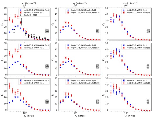
Longitudinal 2PCF profiles for O vi (in physical units, along with velocity scale corresponding to a mean redshift of 0.3). The left panels show the comparison between the two feedback models, ‘WIND + AGN’ and ‘WIND’-only. On the middle and right panels, we show the comparison between the ‘fg11’ and ‘ks19q18’ UVBs for ‘WIND + AGN’ (middle panels) and ‘WIND’-only (right panels) feedback models. The top, middle, and bottom panels show the 2PCF profile for O vi absorbers having column densities N(O vi) > 1013, 1013.5, and 1014 cm−2, respectively. In panel (a), we also plot the longitudinal clustering of O vi absorbers from observations using HST-COS spectra (Danforth et al. 2016).
For the sake of completeness, we also compare the simulated clustering amplitudes with that observed for the HST-COS sample (Danforth et al. 2016) in panel (a). It is to be noted that the sample of O vi absorbers used to compute the observed clustering is not based on column density thresholds. The weakest absorber detected in the sample has N(O vi) ≃ 1013cm−2 (see fig. 10 of Danforth et al. 2016). We compare this observed 2PCF profile with the simulated 2PCF profile with absorbers having N(O vi) > 1013 cm−2. Within the errorbars, the observed O vi clustering amplitude matches well with simulations up to a length-scale of 2 Mpc (matches better for the ‘WIND’ model at ≈0.7 Mpc and with ‘WIND + AGN’ model at ≈0.4 Mpc). We find an excess of positive clustering at scales up to 6 Mpc in the observations as opposed to ≃2 Mpc in the case of simulations. This suggests either an underprediction of the volume filling of metals or a deficiency in the large-scale power if O vi absorbers predominantly originate from the circumgalactic medium (CGM) of galaxies in the simulations. Also, we use constant SNR in our simulations. For proper comparison with observations, we need to consider SNR distribution and wavelength-dependent absorption line detection sensitivity for each observed spectrum (as in the case of Maitra et al. 2022, for Ly α absorbers). Such an exercise is not needed for this study as we are mainly interested in probing the difference in the clustering properties of the two simulations.
It is also evident from the figure that beyond 2 Mpc the two simulations produce nearly identical 2PCFs for all three O vi column density thresholds considered. As the cosmological parameters and initial conditions are the same for both the simulations, it is most likely that beyond 2 Mpc the clustering is dominated by the cosmological parameters for the feedback models considered in our simulations.
3.3 Effect due to photoionizing backgrounds
In the case of Ly α forest, it has been found that small-scale clustering for a given N(H i) threshold depends on the assumed UVB (Maitra et al. 2020, 2022). In particular, it has been found that the clustering is stronger when the ionization rate is higher, as in this case, for a given N(H i) one probe higher density range. Here, we explore whether such a dependence is clearly present in the case of O vi absorbers as well. In panels (b), (e), and (h), we plot the 2PCF profiles for two different UVBs for the ‘WIND + AGN’ feedback models for three N(O vi) thresholds.
As can be seen from table 1 of Mallik et al. (2023), the O vi photoionization rate is 2.8 times higher for the ‘ks19q18’ UVB compared to that of ‘fg11’. How this affects the number of absorbers and individual O vi column density measurements depends on the physical state of the gas (i.e. temperature and density). It is clear from Table 1 that in the case of ‘WIND + AGN’ models, there is a substantial increase in the number of absorbers when we use ‘fg11’ background. The lower photoionization rate typically increases the O vi ion fraction, and this leads to the enhancement in the column density and number of weak absorption components above the detection threshold. However, the effect of UVB on the number of detected absorbers is less significant in the case of ‘WIND’-only models. This is because most of the O vi absorbers detected in this case originate from high-density regions where collisional excitation has a stronger influence. We once again refer the readers to section 2 of Mallik et al. (2023) for details.
It is clear that the effect of UVB is seen only for r∥ ≤ 0.8 Mpc for simulations considered here. In this range, the 2PCF amplitudes are, in general, slightly larger in the case of ‘ks19q18’ background. Even though the amplitudes of 2PCF are large in the case of ‘WIND’-only feedback models, the errors are also larger. Within the measurement errors, the UVB dependence, even at small scales, is not that significant compared to what we see in the case of ‘WIND + AGN’ feedback models. This behaviour is, again, commensurate with the finding of Mallik et al. (2023) that CDDF of O vi depends weakly on UVB for the ‘WIND’-only feedback models while it shows a strong dependence in the case of simulations with ‘WIND + AGN’ feedback (also see Table 1). It is also evident that the difference in the 2PCF at a small scale found between two feedback models for a given UVB is much larger than the scatter introduced by changing UVB for a given feedback model. This again indicates that the clustering at small scales may more strongly depend on the feedback model (specifically on what is the temperature, density, and metallicity of the regions where O vi absorption originates) than on the assumed UVB.
It is evident from Table 1 that there are more O vi systems and Voigt profile components identified when we use ‘fg11’ UVB in the case of ‘WIND + AGN’ models. A significant difference in the two-point correlation is seen only over r∥ < 1 Mpc. To understand this, we explore the simulation results for z ∼ 0.3 in some detail. Out of the 20 000 sightlines considered, we identify 5765 components when we use ‘ks19q18’ UVB and 12 662 components for ‘fg11’ UVB, with 3446 components being common between the two UVBs. When we use the ‘fg11’ UVB, |${\sim} 75~{{\ \rm per\ cent}}$| of the newly detected components are found to be within 2 Mpc of the common absorbers. Around 10 per cent are found close to the common absorbers but with separations more than this. The remaining new absorbers are distributed along sightlines that did not show O vi absorption when we use ‘ks19q18’ UVB. Most of the newly detected O vi systems also require multiple Voigt profile components. This explains why the effect of UVB is restricted to small scales. This, together with the lack of such a trend in ‘WIND’-only simulations, indicates that the exact range over which the effect of UVB can be seen may depend on the metal distribution in the simulations. This may depend on the mass resolution of the simulations and how well the parameters influenced by the feedback implementations are converged.
4 DISCUSSION
The observed column density distribution has been frequently used to constrain different feedback processes in hydrodynamical simulations. Recently, it has been shown that the simulated CDDF is also influenced by the assumed UVB. Thus, by only using the observed CDDF one will not be able to lift the degeneracy between the effect of feedback and UVB used in the simulations.
Considering hydrodynamical simulations with two different feedback processes and two different UVBs, we show that observed clustering of O vi at different scales can be used to constrain the photoionizing background, feedback processes, or cosmological parameters. In the models considered here, the effect of UVB is restricted to very small scales (<1 Mpc) compared to the scales that are influenced by feedback processes (1–2 Mpc). Our results suggest that by combining CDDF with 2PCF, one will be able to place better constraints on the feedback processes and the UVB.
While arriving at these results, we have not incorporated the effect of the ionizing radiation originating from local sources, in particular for O vi absorption originating from the CGM. Upton Sanderbeck et al. (2018) have shown that local stellar high-energy radiation from Milky Way-like galaxies influences the ionization state of the gas up to 10–100 kpc. Oppenheimer et al. (2018) have explored the influence of flickering AGNs on the ionization state of metals in the CGM. They suggested, under plausible models, that this could increase the O vi column densities around star-forming galaxies out to 150 kpc. Thus, it appears that the inclusion of the local ionizing radiation fields in the star-forming regions could not have affected the above results.
The length-scale up to which a feedback model can influence the 2PCF may also depend on the strength of the feedback assumed in the model. Recently, SIMBA simulations, including bipolar jet-mode feedback, have shown that widespread disturbances can be introduced. Such feedback models not only heat the matter over large scales but can also spread metals to lower density regions. Bradley et al. (2022) have shown the introduction of such feedback naturally reproduces the observed O vi CDDF (in particular at the high column density end). As discussed in Mallik et al. (2023) unlike other simulations, in SIMBA simulations with jet-mode feedback, a high fraction of gas (i.e. |${\sim} 70~{{\ \rm per\ cent}}$| compared to ∼30 per cent found in other simulations) is present in the WHIM phase from which most of the high ions originate. Our study indicates that the 2PCF of O vi obtained for the ‘WIND + AGN’ model that spreads metals and influences the physical state of gas over a larger scale shows reduced amplitude compared to that of the ‘WIND’-only models. Therefore, the 2PCF predicted by the SIMBA simulations run with jet feedback is expected to be different from that obtained from other simulations. Therefore, simultaneous comparison of CDDF and 2PCF of models with the corresponding observed distributions is important to gain much better insight into the feedback processes.
The clear segregation in scales over which different effects influence the inferred 2PCF seen for the two simulations used here needs to be further explored using models with a wider range of feedback prescriptions. In particular, it will be interesting to establish the existence of different scales over which UVB and feedback processes influence the two-point correlation using the whole range of feedback models considered by Nelson et al. (2018) for studying the large dispersion they produce in CDDF.
It is also known that how effectively the UVB is controlling the ionization fraction of a given ion depends on the gas temperature. For example, if O vi absorption originates predominantly from the collisionally ionized gas, then we expect the dependence of the UVB to be minimal. Sherwood simulations are known to produce higher temperatures for the O vi absorbers (see Mallik & Srianand 2024, for discussion on this). Because of the mass resolution of the simulations used here, metal pollution from low-mass haloes (i.e. Mhalo < 108 M⊙) is not present. It is also important to explore the effect of metal enrichment by low-mass haloes on the clustering analysis. The above-mentioned exercise using TNG simulations will allow us to address these issues as well.
Lastly, we notice that the observed 2PCF for O vi absorbers has positive signals up to ∼6 pMpc. However, simulations considered here have positive signals only up to ∼3 pMpc. It will be important to understand the origin of this difference. As mentioned above, correlation analysis performed using a wide range of simulation suites available in the IllustrisTNG simulations will be very useful in this regard.
ACKNOWLEDGEMENTS
We thank the referee and the scientific editor for their constructive comments. SM acknowledges support from PRIN INAF – NewIGM programme. We acknowledge the use of HPC facilities PERSEUS and PEGASUS at IUCAA. We would like to extend our gratitude to Kandaswamy Subramanian for useful discussion and Prakash Gaikwad for providing the automated Voigt profile fitting code viper. We would also like to mention that the Sherwood simulations were performed using the Curie supercomputer at the Tre Grand Centre de Calcul (TGCC) and the DiRAC Data Analytic system at the University of Cambridge, operated by the University of Cambridge High Performance Computing Service on behalf of the STFC DiRAC HPC Facility (www.dirac.ac.uk). This was funded by BIS National E-Infrastructure capital grant (ST/K001590/1), STFC capital grants ST/H008861/1 and ST/H00887X/1, and STFC DiRAC Operations grant ST/K00333X/1. DiRAC is part of the National E-Infrastructure.
DATA AVAILABILITY
The observed O vi clustering is taken from Danforth et al. (2016) and the HST-COS data products used to compute this clustering can be accessed from https://archive.stsci.edu/prepds/igm/.
Footnotes
Please refer to section 2.2 of Mallik et al. (2023) for the definition of different phases.
