


ABSTRACT
Machine learning photo-z methods, trained directly on spectroscopic redshifts, provide a viable alternative to traditional template-fitting methods but may not generalize well on new data that deviates from that in the training set. In this work, we present a Hybrid Algorithm for WI(Y)de-range photo-z estimation with Artificial neural networks and TEmplate fitting (hayate), a novel photo-z method that combines template fitting and data-driven approaches and whose training loss is optimized in terms of both redshift point estimates and probability distributions. We produce artificial training data from low-redshift galaxy spectral energy distributions (SEDs) at z < 1.3, artificially redshifted up to z = 5. We test the model on data from the ZFOURGE surveys, demonstrating that hayate can function as a reliable emulator of eazy for the broad redshift range beyond the region of sufficient spectroscopic completeness. The network achieves precise photo-z estimations with smaller errors (σNMAD) than eazy in the initial low-z region (z < 1.3), while being comparable even in the high-z extrapolated regime (1.3 < z < 5). Meanwhile, it provides more robust photo-z estimations than eazy with the lower outlier rate (|$\eta _{0.2}\lesssim 1~{{\ \rm per\ cent}}$|) but runs ∼100 times faster than the original template-fitting method. We also demonstrate hayate offers more reliable redshift probability density functions, showing a flatter distribution of Probability Integral Transform scores than eazy. The performance is further improved using transfer learning with spec-z samples. We expect that future large surveys will benefit from our novel methodology applicable to observations over a wide redshift range.
1 INTRODUCTION
Wide-field imaging surveys are a fundamental driver of astronomical discovery in the fields of galaxy evolution and cosmology. Galaxy redshifts are a key component in the application of the large-survey data, representing the measurement of galaxy distances. They are crucial for identifying objects present in the early Universe, tracing the evolution of galaxy properties over cosmic time and constraining cosmological models.
There are two major methods for determining galaxy redshifts: using spectroscopically identified spectral line features (spectroscopic redshifts, hereafter spec-z’s), or via multiband photometry (photometric redshifts, Baum 1962; Butchins 1981; Connolly et al. 1995; Hildebrandt et al. 2010, hereafter photo-z’s). Spec-z’s are typically much more accurate but more observationally costly than photo-z’s; there is a trade-off between the sample size of a data set and the precision of redshift estimates (Salvato, Ilbert & Hoyle 2019). In the context of upcoming large surveys, extragalactic astronomy will benefit from photo-z estimation at an unprecedented level as follow-up spectroscopy can never keep pace with present and future large imaging surveys, for example, the Vera C. Rubin Observatory’s Legacy Survey of Space and Time (LSST; LSST Science Collaboration 2009), the Dark Energy Survey (DES; Dark Energy Survey Collaboration 2016), the Nancy Grace Roman Space Telescope (Spergel et al. 2015), the JWST (Finkelstein et al. 2015), the Hyper Suprime-Cam Subaru Strategic Program (Aihara et al. 2018, 2022), the Euclid mission (Euclid Collaboration 2020), and the Kilo-Degree Survey (KiDS; Hildebrandt et al. 2021). Thus, efficient and accurate estimation of photo-z’s is a topic that has fundamental importance in various fields of research.
There are two main approaches to photo-z estimation. One is the template-fitting method, a kind of model-fitting approach (e.g. Arnouts et al. 1999; Benítez 2000; Bolzonella, Miralles & Pelló 2000; Feldmann et al. 2006; Brammer, van Dokkum & Coppi 2008; Eriksen et al. 2019), while the other is the data-driven method of empirical modelling based on spec-z’s – machine learning (ML, e.g. Carrasco Kind & Brunner 2013; Graff et al. 2014; Almosallam, Jarvis & Roberts 2016; Sadeh, Abdalla & Lahav 2016; Izbicki, Lee & Freeman 2017; Cavuoti et al. 2017a; Graham et al. 2018). The main advantage of template fitting is it can be generally applied at any redshift. It is, however, unable to learn from data to improve performance, which is fundamentally constrained by the template set. In contrast, the benefit of the data-driven method is generalization to ‘unseen data’ via learning from the given data set. It potentially outperforms template fitting by learning a mapping from photometry to redshift and bypassing potentially unrepresentative templates. This also reduces the computational demands for photo-z estimation compared to the one-on-one matching between individual objects and templates. However, it typically can not be expected to work outside the redshift range present in the spec-z training set.
Template-fitting methods, in which photo-z’s are derived from matching the broad- or medium-band photometry of an observed galaxy to pre-defined SED templates, have proven to be very useful. The template library commonly employed for photo-z study has been updated over the past few decades, exploiting observed (e.g. Bolzonella et al. 2000; Ilbert et al. 2006, 2009; Salvato et al. 2009) and synthetic (e.g. Carnall et al. 2018; Battisti et al. 2019; Boquien et al. 2019; Bellstedt et al. 2020) galaxy SEDs. With this method we can estimate photo-z’s for any region of colour space at any redshift. However, the photo-z estimation with this technique still relies on a limited set of pre-defined templates (which may be more or less representative of the observed galaxy population) as well as the fitting algorithm. The template-fitting method is likewise often computationally intensive and inappropriate for the ongoing and future large survey projects, which would require feasible solutions for analysing unprecedentedly large data sets in peta-scale regimes depending on the science cases.
ML techniques employ an algorithmic model for learning from a given data set to capture its underlying patterns and then utilize the learned model to make predictions on new data. They are able to learn from large volumes of data and automatically capture inherent patterns therein that may not be apparent to humans. In the context of photo-z prediction, this represents a promising route to estimate redshifts from an unprecedentedly huge data set composed of multiband photometric data associated with spec-z information.
Different ML algorithms have been utilized in previous works on photo-z estimation. Carrasco Kind & Brunner (2013) introduced a photo-z method based on prediction trees and random forest (RF) techniques (Breiman & Schapire 2001). The Multi Layer Perceptron with Quasi Newton Algorithm (MLPQNA; Brescia et al. 2013, 2014) contributed to many photo-z works as an excellent demonstration of feed-forward neural networks. Sadeh et al. (2016) applied multiple ML methods to their model that utilizes artificial neural networks (ANNs) and boosted decision trees, while Jones & Singal (2017) presented a support vector machine (SVM) classification algorithm for photo-z estimation. These photo-z based ML methods are generally trained to learn the complex relationship between photometry and distance of observed galaxies. Most of them have been actually tested on the publicly available data from the PHoto-z Accuracy Testing (phat) program (Hildebrandt et al. 2010; Cavuoti et al. 2012), performing comparably in terms of photo-z accuracy.
ANNs have been one of the most popular ML algorithms used in photo-z study, which are inspired by the biological neural networks of the human brain (Mcculloch & Pitts 1943; Hopfield 1982). They can theoretically approximate any complex function based on the Universal Approximation Theorem (Cybenko 1989; Hornik 1991), allowing a model to map nonlinear relationships between photometry and redshift. In particular major advances have been produced exploiting the flexibility of fully connected neural networks (FCNNs), in which each neuron in one layer is connected to all neurons in the next layer.
A major stumbling block for photo-z based ML approaches is incompleteness in spectroscopic training samples commonly used as the ground truth redshift. This limitation could prevent a trained model from functioning as intended, that is, generalizing robustly to new examples outside the training set. In particular, spec-z catalogues used for training are typically biased towards the bright part of the magnitude parameter space and are incomplete for high-z objects as well. This also explains why photo-z estimations at high redshifts still rely on existing template fitting methods rather than ML techniques, although they are more common at z ≲ 1. Moreover, training-based methods do not generally allow for reliable extrapolation beyond a known range of data that can be well represented by the training data. The target redshift range for ML is therefore limited to low-z regions of sufficient spectroscopic completeness with higher success rate in obtaining accurate redshifts for brighter objects.
Furthermore, both template- and ML-based photo-z codes generally fall short in producing valid probability density functions (PDFs) of redshift, which fully characterize the results of photo-z estimation (Schmidt et al. 2020). Per-galaxy photo-z PDFs have been commonly applied to estimate the ensemble redshift distribution N(z) of a sample of galaxies, an estimator critical to cosmological parameter constraints from weak gravitational lensing analysis (e.g. Mandelbaum et al. 2008; Sheldon et al. 2012; Bonnett et al. 2016; Hildebrandt et al. 2017). Schmidt et al. (2020) demonstrated the vulnerability of each single model to a specific flaw in the population of output PDFs in spite of the precise photo-z point estimates. We still lack a model that can produce well-calibrated redshift PDFs and that can be readily adapted to new studies of galaxy evolution and cosmology.
Wolf (2009) proposed an example solution for producing accurate redshift distributions from stacked PDFs, although addressing not typical galaxies but specifically quasars under certain conditions. Combining χ2 template fits and empirical approaches likely preserve both benefits in one framework; empirical training sets can complement unreliable PDFs generated with the χ2 technique based on imperfect templates if matching the distribution and calibration of query samples. This, however, essentially requires an appropriate treatment of error scale used for smoothing the appearance of samples in feature space and controlling the width of derived PDFs.
Traditional ML approaches have generally delivered better performance than template-based methods within the range of training spec-z coverage (Newman & Gruen 2022). The trade-off between the strengths of ML and template-fitting inspires the hybridization of their distinctive advantages. Training the model on simulated photometry is one strategy to overcome the challenges of assembling a complete, reliable and unbiased training sample of sufficient size. Artificial SED samples are often generated using a stellar population synthesis (sps) code with arbitrary selection of free parameters (e.g. Eriksen et al. 2020; Ramachandra et al. 2022). Zhou et al. (2021) applied a set of best-fitting SEDs for the COSMOS catalogue using the template fitting code lephare, produced based on typical sps spectra (Bruzual A. & Charlot 1993; Bruzual & Charlot 2003). A complete training set of simulated galaxies should compensate for the sparse sampling of spec-z data allowing for interpolation between spectroscopically observed objects and even extrapolation to the faintest ones (Newman & Gruen 2022). The fidelity of the mock training samples is still liable to many stellar evolution uncertainties that have long plagued sps models (Conroy 2013). Constructing such an ideal SED data set requires further improvements to sps models and to our knowledge of the underlying galaxy population.
Alternatively, the template-fitting code eazy (Brammer et al. 2008) provides more flexible galaxy SEDs, which fits a linear combination of basic spectral templates to the observed photometry on-the-fly. They developed a minimal template set of synthetic SEDs representing the ‘principal components’, following the template-optimization routines introduced by Blanton & Roweis (2007). The template set is calibrated with semi-analytical models rather than biased spectroscopic samples, which are complete to very faint magnitudes, along with a template error function to account for wavelength-dependent template mismatch. The applicability of eazy to diverse redshift coverage has been demonstrated with a plethora of photometric catalogues (e.g. Treister et al. 2009; Wuyts et al. 2009; Cardamone et al. 2010; Muzzin et al. 2013; Nanayakkara et al. 2016; Straatman et al. 2016; Strait et al. 2021). In particular, the reliability of eazy photo-z’s was thoroughly assessed with comprehensive photometric samples presented by Straatman et al. (2016, hereafter S16), which include medium-bandwidth filters from the FourStar galaxy evolution (ZFOURGE) surveys.
In this work, we present a novel hybrid photo-z method that combines template-fitting and data-driven approaches to exploit the best aspects of both. Our photo-z network is trained with mock photometric data generated based on the ensemble of template SEDs provided by eazy. This is particularly motivated by exploiting knowledge of galaxy SEDs at low-z, where template fitting is assumed to be reliable, and applying their rest-frame SEDs to a higher redshift range. The full training set of mock SEDs is thus generated by redshifting best-fitting SEDs derived with eazy for the S16 photometric catalogue objects of z ≲ 1, whose simulated redshifts are distributed in a broader range up to z = 5. We develop photo-z convolutional neural networks (CNNs; Lecun et al. 1998; LeCun, Huang & Bottou 2004) optimized to simultaneously produce both a well-calibrated set of redshift PDFs and accurate point estimates. The trained model is tested with updated S16 spectroscopic samples, whose performance is evaluated based on photo-z metrics commonly used for measuring the quality of both output PDFs and the corresponding point estimates.
Our ML strategy benefits from recent advances in the field of domain adaptation (Csurka 2017; Wang & Deng 2018; Wilson & Cook 2020), which allows a model to learn domain-invariant features shared between discrepant data distributions. The simulation-based ML model here is trained with synthetic data, which can be further advanced by transfer learning (Pan & Yang 2010), where a model pre-trained on one task is re-purposed on another related task. Pre-training the feature extraction layers on a large external data set then fine-tuning on a smaller training set alleviates overfitting compared to simply training from scratch on the small data set. We can thus fine-tune the simulation-based photo-z network with a limited amount of spectroscopic data by re-training the last layers on real data sets with spec-z information (Eriksen et al. 2020). This optimization scheme in principle aids in correcting the gap between mock and observed training samples.
Our novel approach is to ‘extrapolate’ training methods outside their initial redshift ranges from the viewpoint of the original template fits. Training with domain adaptation can be performed on high-z simulated data by capturing a realistic range of galaxy SED properties determined from reliable low-z data. In place of spectroscopic data, we leverage the demonstrated accuracy of template fitting, overcoming the traditional redshift limitation of ML photo-z codes. In essence, the CNN-based hybrid model is thus designed to function as an efficient emulator of eazy. The interpolative nature of supervised ML approaches could even infer photo-z point estimates more precisely and robustly than those provided by the original template-based method. Incorporating the flavour of template fitting into the ML framework potentially improves the quality of photo-z PDFs as well. Ultimately, we aim to improve photo-z estimation for JWST photometry, which will have coverage at redder wavelengths than previously available.
This paper is organized as follows. In Section 2, we present the photometric catalogues used in this work. In Section 3, we detail our method for producing mock photometric data (with a noise model) via simulations. Section 4 describes the development of our ML photo-z networks and the framework for evaluating their performance. Section 5 presents results on testing different photo-z models on the ZFOURGE catalogue data and comparing their performance in photo-z and PDF metrics commonly used for major photo-z studies. In Section 6, we discuss some of the issues raised by the work. Finally, in Section 7, we summarize the work and discuss future prospects. Throughout this paper, we assume a lambda-cold dark matter cosmology with ΩM = 0.3, ΩΛ = 0.7, and H0 = 70 km s−1 Mpc−1.
2 CATALOGUE DATA
This work introduces a hybrid photo-z based ML method that benefits from the template-fitting algorithm of eazy, aimed at deriving photo-z PDFs of galaxies extracted from the ZFOURGE photometric catalogues (Straatman et al. 2016). ZFOURGE data products comprise 45 nights of observations with the FourStar instrument (Persson et al. 2013) on the 6.5 m Magellan Baade Telescope at Las Campanas in Chile. It observed three survey fields including Chandra Deep Field South (CDFS; Giacconi et al. 2002), COSMOS (Scoville et al. 2007), and UKIRT Ultra Deep Survey (UDS; Lawrence et al. 2007) with five near-IR medium-bandwidth filters, J1, J2, J3, Hs, and Hl, along with broad-band Ks. Pushing to faint magnitude limits of 25–26 AB achieves the mass completeness limit of ∼108 M⊙ at z ≲ 1, also advancing the study of intermediate to high redshift objects.
S16 includes data from publicly available surveys at 0.3-|$8 \,\mathrm{\mu }\mathrm{m}$|, constructing comprehensive photometric catalogues, each with a total of 39 (CDFS), 36 (COSMOS), and 27 (UDS) medium- and broad-band flux measurements. The individual objects were cross-matched with the compilation of publicly available spec-z catalogues provided by Skelton et al. (2014) as well as the first data release from the MOSFIRE Deep Evolution Field (MOSDEF) survey (Kriek et al. 2015) and the VIMOS Ultra-Deep Survey (Tasca et al. 2017). These samples have been used to demonstrate the benefit of including the FourStar medium bands in the input for improving the photo-z accuracy with a better sampling of galaxy SEDs (Straatman et al. 2016).
Throughout, the catalogue data utilized for this work are limited to objects with a use flag of 1, which represents reliable data with good photometry and a low likelihood of contamination with stars or blending with another source. These sources are obtained from regions of the images with sufficiently high signal to noise (S/N). We thus construct test catalogue samples with use = 1 and total Ks-band magnitude <26, providing the galaxy population that can be used in large statistical studies. Our main target objects are high-z galaxies of z ≳ 1.3, whose photo-z estimations have not been well explored by ML methods. We set the lower limit to 1.3 as that is a typical bound for which spec-z’s are incomplete, since the galaxy optical light is redshifted in to the near-IR. The model is none the less required to make predictions across the whole redshift range (including lower z′s), since we cannot exclusively select high-z objects a priori from real observations. Our spec-z samples are therefore limited only with an upper bound of 5, which are adopted as a test set for evaluating the model’s performance on the broad redshift range between 0 < zspec < 5.
Additionally, we incorporate ancillary spec-z data from the latest releases of several surveys into our original S16 catalogue, with a matching radius of 1 arcsec. All the catalogues are supplemented by the final data releases from the MOSDEF (Kriek et al. 2015) and Multi-Object Spectroscopic of Emission Line (MOSEL; Gupta et al. 2020; Tran et al. 2020) surveys. The fourth data release from the VIMOS survey of CANDELS UDS and CDFS (VANDELS; Garilli et al. 2021) provides auxiliary spec-z’s for CDFS and UDS, while the ZFIRE survey (Nanayakkara et al. 2016) for COSMOS. We only extract reliable data with the best quality flag individually defined for each survey catalogue.
As a further step, two of the authors (KG and IL) visually inspected spectra where the spec-z and eazy photo-z's differed significantly. We removed objects deemed likely misidentifications, providing sample sizes of 1100 (CDFS), 425 (COSMOS), and 127 (UDS) from the original S16 catalogue. The size of each supplemented sample (z > 1.3) is as follows: 1273 in CDFS, 741 in COSMOS, and 314 in UDS, an increase of 173, 316, and 187, respectively.
3 TRAINING SET OF MOCK PHOTOMETRIC DATA
In this section, we discuss the generation of mock photometric data used for training the ML model. The entire process is divided into two major parts, both of which are important for creating a training sample that can sufficiently cover the colour space occupied by the test sources. Section 3.1 describes the method of producing mock SEDs from eazy best fits for a limited sample of low-z galaxies in S16. In Section 3.2, the noise model is introduced to apply realistic errors to simulated photometry, which allows for the construction of reliable mock photometric data.
3.1 Mock galaxy SEDs
We simulate galaxy SEDs up to z = 5 by redshifting the eazy best-fitting SEDs for low-z objects with zeazy < 1.3 in S16. This enables us to produce SEDs of galaxies in the target redshift range between 1.3 < z < 5 purely based on a galaxy population at lower redshifts. The selection criteria of the low-z sources also ensures the generated sample fully covers typical SED types, since ZFOURGE is very complete to low masses at z ≲ 1.3, where the 80 per cent mass completeness limit reaches down to ∼108–108.5M⊙ (Straatman et al. 2016). We thus first extract eazy best fits for objects with zeazy < 1.3 that are included in the photometric catalogues of S16. The total number of selected low-z sources is 17 891. These empirical SEDs are technically unique, since eazy fits an ensemble of nine representative spectral templates to each set of observed fluxes. The major part of our simulated sample thus consists of typical SED types empirically obtained from low-z observations but assumed to be present at much higher redshifts.
We then artificially redshift these pre-defined SEDs from the limited redshift range of zeazy < 1.3 to simulated redshifts (zsim’s) in a much broader range of 0 < zsim < 5. For each mock SED, a set of simulated wavelength and flux density per unit wavelength (λsim, Fsim) measurements are derived from the eazy output (λeazy, Feazy) with the following equations:
where Deazy and Dsim are the luminosity distance for the observed and simulated galaxies.
The simulated data are generated with a uniform distribution with respect to ζ = log (1 + z), which is adopted as our output variable instead of the simple redshift (Baldry 2018). This adapts to the evaluation scheme commonly used in most photo-z studies, where the redshift estimation error is defined as dζ = dz/(1 + z). Using dζ as a reasonable photo-z error is ascribed to different photometric uncertainties for a given set of broad-band filters, which typically have an approximately constant resolution of R = dλobs/λobs ∼ const., where λobs is an observed wavelength. dζ thus shows a constant error if an observational error of dz purely scales with the filter spacing dλobs, while λobs with (1 + z).
The uniform distribution of simulated ζ’s ensures that the number density of the training data is constant at any ζ, which is required for developing a photo-z network whose error estimations are not biased in the entire redshift range. One of our goals is to build a model that produces reliable redshift PDFs as well as single-point estimates, which is implemented by outputting probabilities for 350 ζ class bins, as described in Section 4.1. We generate multiple mock SEDs from a given low-z source by randomly drawing ζ in each of 35 equally discretized bins, whose resolution is 10 times lower than the output probability vector. The sample size of our mock SEDs consequently results in ∼600 000.
Our knowledge of the underlying galaxy SEDs is exclusively attributable to objects observed with the FourStar medium-band filters. The high number of filters in these photometric data ensures the individuality of each empirical template, which would be otherwise standardized into a small set of simplified representations. This allows us to efficiently generate realistic high-z SEDs even in the absence of large amounts of data about the distant universe. We note that the current framework does not take into consideration the difference in population between low-z and high-z galaxies due to their evolution. Handling this issue in a robust manner is beyond the scope of this paper, but our input fluxes are normalized to remove magnitude information, as described in Section 4.1, which should alleviate the impact on the model’s performance.
3.2 Photometry simulations with noise application
The photometry for the mock SEDs is simulated using a transmission curve for each filter adopted in S16, producing a noiseless flux per unit wavelength |$\bar{F}_{i}$| for the band i. Establishing a realistic photometric sample then requires artificially applying an observational error to each noiseless flux. The fundamental concept of our fiducial noise model (which we call ‘empirical’) is to introduce actual observational noise for one test source t into simulated photometry of each mock SED.
We explore the most appropriate noise realization for a given simulated SED in comparison with the observed data. This requires a measure of similarity in SED shape St between noiseless simulations |$\bar{F}_{i}$| and noised observations |$(\tilde{F}_{i,t},\tilde{E}_{i,t})$|, where |$(\tilde{F}_{i,t},\tilde{E}_{i,t})$| is a set of flux and error observed for the band i from the source t. An approximate SED shape is captured by normalizing all the fluxes and errors of each object by its own Ks-band photometric measurement. Each pair of simulated and catalogue sources are then compared based on these normalized photometric data, |$\bar{f}_{i}$| and |$(\tilde{f}_{i,t},\tilde{e}_{i,t})$| (here we denote normalized data with lower case).
For each mock galaxy, the similarity between |$\bar{f}_{i}$| and |$(\tilde{f}_{i,t},\tilde{e}_{i,t})$| is measured by assuming each simulated flux fi, t follows a Gaussian distribution given a standard deviation |$\tilde{e}_{i,t}$|. eazy also adapts to template mismatch with a rest-frame template error function σte(λ). The total flux uncertainty δfi, t is given by
where λi, rest is the rest-frame central wavelength of the filter i, expressed with the observed wavelength λi as λi, rest = λi/(1 + zsim).
We thus assume |$f_{i,t}\sim N\left(\bar{f}_{i},\left.\delta f_{i,t}\right.^{2}\right)$| to estimate a probability pi, t that the observed |$\tilde{f}_{i,t}$| is realized, given by
The product of fluxes across each band then measures the stochastic similarity of the mock galaxy to the catalogue source t:
where i covers nt broad- and medium-band filters adopted in S16 which do not contain missing values. The similarity measure St consequently needs to be defined in a form that should be generally applicable to comparing any pairs, since the effective number of filters nt is not fixed for all the catalogue sources, dependent on t. One reasonable measurement is given by
which can function as a probability of realization for an object t.
We additionally adopt a magnitude prior p(z|m) following Straatman et al. (2016) for computing a probability of drawing a test source t, expressed as
where mt is the Ks-band apparent magnitude. One catalogue object is randomly picked with a probability P(zsim, t), whose errors |$\lbrace \tilde{e}_{i,t}\rbrace _{i}$| are applied to each simulated SED including its missing values. The noised flux Fi, t is then obtained by denormalizing |$f_{i,t}\sim N(\bar{f}_{i},\tilde{e}_{i,t}^{2})$|.
We also establish simpler noise models to explore the benefit of our empirical one:
Noiseless: all the noiseless simulated fluxes are fed to the photo-z network as inputs, given by |$F_{i}=\bar{F}_{i}$|.
Missing: for each mock SED, we randomly draw one test source from the spec-z catalogue whose missing values for some band filters are directly incorporated into the simulated photometric data.
Const: photometry for each mock SED is performed with a constant noise Ecnt over the entire wavelength range. Ecnt is obtained by assuming an arbitrarily selected S/N for Ks-band photometry, where S/N is a random variable ranging between 3 and 30. Each noiseless flux point then varies following a Gaussian distribution with |$F_{i}\sim N\left(\bar{F}_{i},E_{cnt}^{2}\right)$|, which also reflects the missing values in the same method as the Missing model (ii).
Empirical: our fiducial model.
Fig. 1 shows the simulated photometry for an example mock SED, whose noised fluxes are generated with the four different noise models. The Missing model (ii) drops one flux value as missing, which is represented by the red cross, while the Const model (iii) further adds constant errors to the remaining fluxes. More realistic photometry can be simulated with the Empirical model (iv), where the empirical noise is applied to the noiseless fluxes which is extracted from the test sample.

Simulated photometry with different noise models for the same mock SED. All the simulated fluxes are shown by the circles with error bars, while the crosses represent missing data. The top panels present purely integrated photometry without artificial noise, but without (left) and with (right) some missing values included based on a randomly picked catalogue source. These flux points are drawn from the Gaussian distributions with a constant variance over all wavelengths in the bottom left panel. The bottom right panel exhibits the artificial noise generated from the photometric data of a catalogue source with a similar SED shape.
We then train the CNN models, whose architecture is introduced in Section 4.3, on the different simulated data sets for CDFS, each generated with one of the four noise models. Testing them on the same spec-z catalogue sample allows us to explore the most effective noise model. The performance of each CNN is evaluated with the accuracy σNMAD and the outlier rate η0.2 of photo-z point estimates, as described in Section 4.4. Fig. 1 presents the results, revealing the Noiseless model (i) causes a catastrophic failure in photo-z estimations since the training sample does not contain any errors and missing values in photometric measurements. This can be improved by incorporating missing values into the training set which reflect those of the test sample. The Missing model (ii) achieves much better results of σNMAD ∼ 0.03 and |$\eta _{0.2}\sim 20~{{\ \rm per\ cent}}$| than those of the Noiseless model (i) with σNMAD ∼ 0.4 and |$\eta _{0.2}\sim 60~{{\ \rm per\ cent}}$|.
The Const model (iii) shows further improvements by applying simple artificial noise to the noiseless fluxes, reducing σNMAD and η0.2 to ∼0.013 and |$\sim 2.3~{{\ \rm per\ cent}}$|. Significantly better scores can be obtained as well by training the model on more realistic mock data generated with the Empirical model (iv), which result in σNMAD ∼ 0.009 and |$\eta _{0.2}\sim 1.5~{{\ \rm per\ cent}}$|. These results indicate the empirical noise application shows the smallest disparity between simulations and observations. We therefore conclude that the the Empirical model (iv) can produce mock photometric data which best represents the test catalogue samples. The empirical treatment of noise in the training set further improves the precision of PDFs derived for the query set, which can translate into matching the error scales of the distinct samples (Wolf 2009). Effectively, the combination of our chosen noise model, our loss function, and the non-linearity of the neural networks may allow the model to treat the error scale as a parameter and optimize it such that the smoothing scale of the combined error more effectively matches that of our target data.’
We randomly generate five realizations of empirical noise based on the same mock SED sample for each field. This provides stochastically different photometric samples, each constructed by matching the given simulated galaxies with randomly selected catalogue data following the relative probability P(zsim, t). They are independently used for training different networks, whose predictions are subsequently combined with the ensemble learning method, as discussed in Section 4.7. We note that missing values present in the test catalogue samples are incorporated into the photometry simulation. This allows our training set to intrinsically contain information on the corresponding missing data, which does not require imputing missing values entailed by the test set for evaluating the model’s performance on real data.
4 ML PHOTO-Z MODEL
We can assess the performance of photo-z networks on the S16 test catalogue by first training them with the mock data. Section 4.1 describes the input and output, which are designed for yielding redshift PDFs from normalized photometric data. In Sections 4.2 and 4.3, the architectures of two different photo-z networks are introduced: an FCNN and a CNN-based model hayate. Section 4.4 discusses commonly used evaluation metrics for photo-z point estimates and their PDFs. Section 4.5 describes the fiducial training configuration for each network, whose lower-level output PDFs are combined with the ensemble learning method, as discussed in Section 4.7. In Section 4.6, we discuss the benefit of transfer learning using spec-z’s for further improvements.
4.1 Inputs and outputs
Our training set contains simulated high-z galaxies which mirror the population of low-z ZFOURGE sources; no evolution of the galaxy population is accounted for. We thus remove information on magnitudes from the input, which are critically influenced by the formation and evolution of galaxies and highly correlated with redshift. Each galaxy is consequently identified purely based on its SED shape. Our input variables are thus primarily flux ratios, which are obtained for each galaxy by normalizing photometric measurements with its total Ks-band flux provided by S16. The photometry is a product of stacked FourStar/Ks-band and deep pre-existing K-band imaging. The superdeep image achieves a maximum limiting depth at 5σ significance of 26.2–26.6, 25.5, and 25.7 mag in CDFS, COSMOS, and UDS, respectively. Using the total Ks-band flux as a baseline therefore ensures the normalized data sets are reliably calibrated. A similar scheme has been established by Eriksen et al. (2020) with input fluxes divided with the i-band flux.
Testing a trained model on the spec-z catalogue also requires handling missing values, which are inevitably present in real data. We adopt a standard approach of imputation by a constant value, replacing all missing values in the normalized input data with −1. The negative substitute value can exclusively represent a lack of effective data distinguished from the other flux measurements, which should be zero or more. As depicted in Fig. 1, our missing data replacement strategy, represented by the Missing model (ii) described in Section 3.2, markedly improves the model’s performance compared to other imputation methods. We note that each data point can potentially represent no flux measurement as distinct from a missing value, an important distinction when mapping from photometry to redshifts. Therefore using a zero value is not appropriate as a placeholder for missing data. We could also employ a more complex method to substitute missing values, depending on the individual data set, such as interpolation/extrapolation and k-nearest neighbours. As these approaches generate fake (though plausible) values for imputation, they could potentially degrade the precision of estimated photo-z’s.
The input fluxes are also combined with their observational errors, which are used for weighting each residual between the template and observed fluxes in the eazy fitting algorithm (Brammer et al. 2008). The Supporting Information on the uncertainty of each photometric measurement can enhance the robustness of the colour–redshift mapping predicted by photo-z networks (Zhou et al. 2021). The number of input variables Ninput is thus twice the number of observational filters Nfilter, with Ninput = 76, 70, and 52 for CDFS, COSMOS, and UDS, respectively.
Our ML approach is to cast the photo-z estimation task into a classification problem by binning the target redshift range into discretized classes and returning a list of probabilities by which an example is found in a given target bin. Multiple-bin regression has been used with template fitting methods in the past, but the benefit of this approach has been demonstrated in recent ML photo-z studies (Pasquet-Itam & Pasquet 2018; Pasquet et al. 2019; Lee & Shin 2021), generally improving the photo-z accuracy. In the context of a model’s development, the probabilistic scrutiny of the redshift PDF allows one to explore the causes of poor performance on some specific objects. Reproducing realistic redshift PDFs as well as single-point estimates could potentially contribute to improving cosmological analyses (e.g. Mandelbaum et al. 2008; Myers, White & Ball 2009; Palmese et al. 2020).
Each PDF produced by our ML models is an output of the softmax function, which contains probabilities in ζ = log (1 + z) classes with a uniform distribution within 0 < ζ ≲ 1.8, corresponding to the redshift range 0 < z < 5. The resolution of ζ bins approximates the PDF of z provided by eazy as the output vector. The configuration adopted by Straatman et al. (2016) lets the algorithm explore a grid of redshifts with a step of wz = 0.005(1 + z). The constant ζ bin width can be thus expressed as wζ ∼ wz/(1 + z) = 0.005, which leads the photo-z network to output a vector of 350 probabilities as a PDF of ζ in our target redshift range.
4.2 Optimization of a baseline FCNN model
We select an FCNN as a baseline model, since it is commonly applied in photo-z estimation works. Tables B1 and B2 summarize some previous works which apply FCNNs to photo-z estimation, where the network was trained on spectroscopic samples in most cases. This requires a huge amount of observational data and consequently results in a limited target redshift range up to no more than ∼1–2. The number of filter bands used for photometric data is seldom as many as ∼10 as well, since cross-matching multiple catalogues tends to significantly reduce the sample size.
The updated S16 contains a much larger amount of photometric information with ∼40 filter bands, while our simulation method allows for training networks on sufficient mock data in a broader redshift range up to 5. The architecture of the baseline FCNN should thus reflect the larger-scale configuration with more trainable parameters. Other relevant works that have introduced photo-z based ML models trained with simulations typically adopt huge networks consisting of many layers and neurons: for example, {Ninput: 600: 400: 250 × 13: Noutput} in Eriksen et al. (2020) and {Ninput: 512: 1024: 2048: 1024: 512: 256: 128: 64: 32: Noutput} in Ramachandra et al. (2022). We perform k-fold cross-validation to explore the most appropriate architecture and optimize its hyperparameters by training the models on the simulated data generated with the Empirical noise model (iv), as described in Section 3.2.
Our photo-z code is designed for classifying input photometric data into 350 ζ bins, providing the output vector that represents a PDF of ζ. We thus employ the standard categorical cross-entropy (CCE) loss function (Baum & Wilczek 1987; Solla, Levin & Fleisher 1988)
where yc and sc are the ground truth and the score returned by the softmax function for each class c. The redshift classifier is tuned so that the ζ-prediction accuracy is maximized and the loss is minimized using one-hot encoding with yc = 1 only for a true class.
For each FCNN, we consider two types of hyperparameters relating to the architecture, the number of layers (Nlayer) and the number of neurons in each layer (Nneuron), as well as those relating to the algorithm, namely learning rate and the dropout rate. The latter (algorithmic) parameters are thus optimized for each set of the architectural ones. Fig. 2 shows the results on hyperparameter optimization for the FCNN, presenting the validation accuracy and loss for each combination of Nlayer and Nneuron within the ranges Nlayer ∈ [1, 9] and Nneuron ∈ [1, 500]. The accuracy is defined as the percentage of predicted redshift classes that match with true ones. Note, we do not expect accuracy to reach 100 per cent even when performing well, since we expect scatter into neighbouring redshift bins as photo-z's are intrinsically uncertain, and some redshifts will lie closer to the bin boundaries. Nevertheless, for a fixed validation sample, it is a good relative indicator. We explore other metrics below.
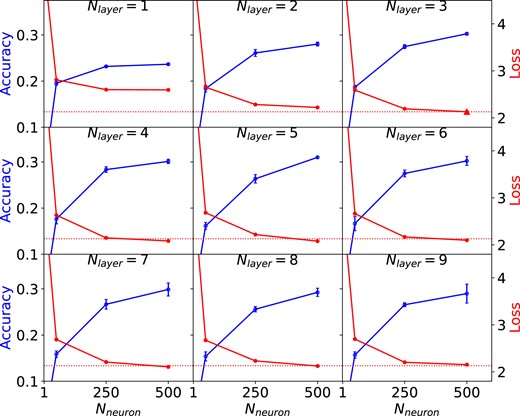
Optimization of architecture and hyperparameters for the FCNN models using fourfold cross-validation. Each panel presents changes in validation accuracy with the number of neurons (Nneuron) as the blue circles (increasing) for a given number of layers (Nlayer). The accuracy score along with its estimation error is given by the mean and standard deviation of the validation accuracy over all folds. The validation loss is also shown by the red circles (decreasing). The dotted horizontal line represents the validation loss obtained from the baseline model, comprising 3 layers with 500 neurons each, which is presented by the red triangle.
Each panel presents changes in accuracy scores with Nneuron for a given Nlayer. We find that the accuracy levels off with increasing Nneuron if the individual layers contain sufficient neurons. This is not affected by the number of layers in general with the accuracy converging to |$\gtrsim 30~{{\ \rm per\ cent}}$|. The minimum loss can be attained by the model with (Nneuron, Nlayer) = (500, 3), with no significant improvement from increasing the number of trainable parameters with larger Nneuron or Nlayer. The architecture of our FCNN model is therefore constructed from three layers with 500 neurons, since a smaller architecture is preferable to a larger one for the same performance. The number of weights to be trained is ∼700 000.
Fig. 3 visualizes the overall architecture of the optimized baseline model with some details excluded. Each layer is followed by ReLU non-linearities, 5 per cent dropout and a batch normalization layer. The input flux ratios along with their observational errors are fed into the network with missing values included, which produces the softmax output of 350 ζ probabilities.
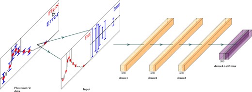
The network architecture of the baseline FCNN classifier. Each figure indicates the output dimension and the model consists of three layers with 500 neurons. Following the intermediate linear layers are ReLU non-linearities, 5 per cent dropout and batch normalization layer. Galaxy flux ratios coupled with normalized observational errors are fed into the photo-z network, which provides the softmax output of 350 probability scores for discretized ζ = log (1 + z) bins.
In the initial exploratory phase of this research other ML techniques were also tested, using a similar hyperparameter optimization strategy. The performance of RFs and SVMs was examined with different sets of hyperparameters: the number of estimators and max depth for RFs and (C, γ) for SVMs, where C controls the complexity of the decision surface, while γ the range influenced by a single data point. Each model was developed with its best hyperparameters, but underperformed the FCNN in that their validation accuracies only reached just under 30 per cent. This indicates that neural networks are more appropriate for our photo-z estimation scheme than other major ML approaches. In particular, with neural networks we have the ability to optimize the loss function for PDF recovery (see discussed in Section 5.1.2).
4.3 Architecture of hayate
We further develop a CNN-based photo-z network and compare the performance of these different ML approaches. As before, the output is a probability vector on discretized redshift bins, which translates the regression problem into a classification task and provides redshift PDFs as well as their point estimates. The output PDF is produced by combining multiple networks independently trained with different configurations, representing an ensemble of stochastic variants for each test object.
We build hayate with the CNN architecture inspired by the VGG neural network (VGGNet; Simonyan & Zisserman 2015), one of the simplest CNN structures commonly used for image classification and object detection. The extended variant of the VGG model, VGG19, consists of 16 convolution layers with 5 max pooling layers followed by three fully connected layers and one softmax layer. It features an extremely small receptive field, a kernel of 3 × 3, which is the smallest size that can capture the neighbouring inputs. Stacking multiple 3 × 3 convolutions instead of using a larger receptive field leads to a deeper network, which is required for better performance (Emmert-Streib et al. 2020). VGG-based models have been successfully applied to astronomical images, for example, for the identification of radio galaxies (Wu et al. 2019), classification of compact star clusters (Wei et al. 2020), and detection of major mergers (Wang, Pearson & Rodriguez-Gomez 2020).
The VGG network is fundamentally designed for handling higher dimensional image data (with multiple colour channels) rather than 1D photometric data. It should be thus applied to photo-z estimation with a much smaller architecture, since the number of trainable parameters originally reaches up to ∼144 million. Zhou et al. (2021) have introduced a 1D CNN used for deriving spec-z’s from spectral data, which can provide some insight into the application of CNNs to photo-z estimation. The input layer includes two channels of spectral data and errors, while the output layer contains multiple neurons representing the probability of each redshift interval. The spec-z analysis is thus performed as a classification task using the feature maps obtained through two convolutional layers, which are followed by two fully connected layers. The number of parameters is consequently far less than that of a CNN commonly used for image processing, totalling no more than ∼350 000.
The task of photo-z prediction can be treated in the same fashion but with input flux and output probability vectors of lower resolution than spec-z. We construct hayate as a simplified variant of the VGG network, whose architecture is illustrated in Fig. 4. The input 2 × Nfilter matrix involves two rows of flux ratios and normalized observational errors, convolved with a kernel of 2 × 3 using zero padding of size 1 and followed by the 3 × Nfilter matrix. Adopting zero padding in the column direction, we then convolve it with a kernel of 3 × 3 to obtain a 1D vector of size Nfilter. The major components are a following sequence of six convolutional layers with 32, 32, 64, 128, 256, and 512 kernels each. The fundamental concept of the VGG network is particularly reflected by a 1D kernel of size 3 used for a convolution operation in each layer. We basically connect the convolutional layers with batch normalization, dropout, and 1D max pooling layers. A fully connected layer is set with 350 neurons in the end, each outputting a softmax probability of finding an object at a given ζ.
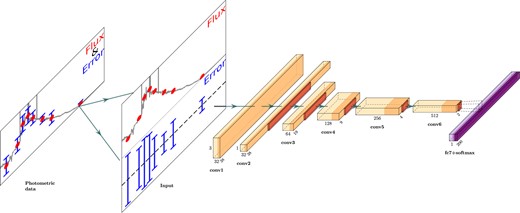
Architecture of hayate. The overall structure consists of six convolutional layers (yellow) with 32, 32, 64, 128, 256, and 512 kernels each. The input 2 × Nfilter matrix contains two rows of flux ratios and normalized observational errors. In the first layer, we convolve the input with a kernel of 2 × 3 using zero padding of size 1. The convolution operation in the following layer then performs on the 3 × Nfilter matrix with a kernel of 3 × 3, outputting a 1D vector of size Nfilter by adopting zero padding in the column direction. Each remaining layer is set with a 1D kernel of size 3, which reflects the fundamental concept of the VGG network. All the convolutional layers are connected with batch normalization, dropout, and 1D max pooling layers except for the first one that lacks a max pooling operation. We set the last layer to a fully connected output layer with 350 neurons, each providing a softmax probability score for a given ζ class.
We have explored more efficient architectures in supplementary experiments, only to conclude that the one mentioned above should perform best among several simple CNNs. We also note that the number of trainable weights for hayate is approximately the same as that of the baseline FCNN described in Section 4.2.
4.4 Evaluation metrics
All the ML photo-z’s are estimated from the redshift PDFs in the same method as implemented in eazy by Straatman et al. (2016). Each point estimate is obtained by marginalizing exclusively over the peak of the redshift PDF which shows the largest integrated probability. This adapts to the degeneracy of template colours with redshift, which produces a PDF with multiple peaks.
The quality of photo-z estimates is evaluated based on the residuals with respect to their spec-z’s, which are given by
where zphot and zspec are photometric and spectroscopic redshifts. Each ML photo-z is immediately recovered from a point estimate of ζ, expressed as zphot = eζ − 1. We employ the following commonly used indicators as statistical metrics to evaluate the model’s performance in single-point estimations:
- σNMAD: normalized absolute median deviation of Δz, described aswhich is robust to Δz outliers.(10)$$\begin{eqnarray} \sigma _{\textrm {NMAD}} & = & 1.48\times \mathrm{ median}(|\Delta z|), \end{eqnarray}$$
Outlier rate η0.2: percentage of outliers, defined as test data with |Δz| > 0.2.
We also use the probability integral transform (PIT; Polsterer, D’Isanto & Gieseke 2016) to properly estimate the calibration of the redshift PDF P(ζ) generated by different photo-z models, which is defined by
where ζspec, t corresponds to the true redshift of the test source t. If the predicted PDFs are well calibrated with respect to the spec-z’s, the histogram of the PIT values, or its PDF f(x), is equivalent to the uniform distribution U(0, 1). The flat distribution indicates that the predicted PDFs are neither biased, too narrow nor too broad. Conversely, underdispersed and overdispersed PDFs exhibit U-shaped and centre-peaked distributions, respectively, while a systematic bias present in the PDFs is represented by a slope in the PIT distribution.
The following evaluation metrics are used for quantifying the global property of output PDFs:
- CvM: score of a Cramér-von Mises (Cramér 1928) test,where F(x) and FU(x) are cumulative distribution functions (CDFs) of f(x) and U(0, 1), respectively. This corresponds to the mean-squared difference between the CDFs of the empirical and true PDFs of PIT.(12)$$\begin{eqnarray} \mathrm{ CvM}=\int _{-\infty }^{\infty }[F(x)-F_{U}(x)]^{2}\mathrm{ d}F_{U}, \end{eqnarray}$$
- KL: Kullback–Leibler (Kullback & Leibler 1951) divergence,which is a statistical distance representing the information loss in using f(x) to approximate U(0, 1). An approximation f(x) closer to U(0, 1) thus shows a smaller KL.(13)$$\begin{eqnarray} \mathrm{ KL}=\int _{-\infty }^{\infty }f(x)\mathrm{ ln}\left(\frac{U(0,1)}{f(x)}\right)\mathrm{ d}x, \end{eqnarray}$$
The reliability of individual PDFs with respect to spec-z’s is represented by the continuous ranked probability score (CRPS; Hersbach 2000; Polsterer et al. 2016), which is given by
where Ct(ζ) and Cspec, t(ζ) are CDFs of Pt(ζ) and ζspec, t for the source t, respectively. Cspec, t(ζ) here corresponds to the CDF of δ(ζ − ζspec, t)
where H(ζ − ζspec, t) is the Heaviside step-function, which gives 0 for ζ < ζspec, t and 1 for ζ ≥ ζspec, t. It reflects the simplest form for the unknown true distribution of ζ, given by the Dirac Delta function between ζ and ζspec, t. The CRPS thus represents the distance between Ct(ζ) and Cspec, t(ζ), or the difference between the empirical and ideal redshift PDFs. We thus assess the reliability of individual output PDFs with the median value of crps, which is robust to outliers than their mean value:
- CRPS: median of all CRPS values obtained from a sample,(16)$$\begin{eqnarray} \mathrm{CRPS}=\underset{t}{\mathrm{median}}({\it crps}{}_{t}). \end{eqnarray}$$
We introduced the CRPS metric primarily because it can be used as part of the ANN optimization process.
Table 1 summarizes the characteristics of these indicators. In summary, σNMAD and CRPS reveal the quality of individual outputs while η0.2, KL, and CvM represent the global property obtained from the distribution of their key attributes.
Summary of evaluation metrics. We employ σNMAD and η0.2 for measuring the accuracy of photo-z point estimates, while KL, CvM, and CRPS are responsible for assessing the quality of photo-z PDFs.
| Indicator | Target to be evaluated | Responsibility | Key attribute | Measurement |
|---|---|---|---|---|
| σNMAD | zphot point estimate | zphot precision | Δz [equation (9)] | Median of |Δz| |
| η0.2 | Rate of catastrophically wrong zphot | Outlier rate of Δz with |Δz| > 0.2 | ||
| KL | P(zphot) | Calibration of produced P(zphot) | x: PIT [equation (11)] | Divergence of PIT distribution f(x) from uniformity |
| CvM | Dissimilarity between CDF of f(x) and identity line | |||
| CRPS | Reliability of P(zphot) with respect to zspec | crps [equation (14)] | Median of crps |
4.5 Training process
The mock photometric data are divided into three parts representing training, validation and test data sets. The test sample contains 20 per cent of the whole set of simulated galaxies, while the rest is split into the training and validation sets with 70 per cent and 30 per cent of the remaining data randomly selected, respectively. The individual networks are trained with a joint loss that combines the CCE loss LCCE and the CRPS loss LCRPS, given by equations (8) and (14), respectively. The CCE loss is frequently used for multiclass classification problems, responsible for the accuracy of single point estimates. The CRPS loss can function as a penalty for failing to produce reliable PDFs, which would be otherwise neglected in a classification task with the single CCE loss.
The joint loss is optimized by an Adam optimiser (Kingma & Ba 2015) in the training process, which is given by
where α and β are the weights to the linear combination of the CCE and CRPS losses. We first explore the appropriate values for α and β in a pre-training process so that LCCE and LCRPS equivalently contribute to the total at loss convergence with αLCCE ≃ βLCRPS. This is achieved by updating them after each training epoch j with the following equations:
where αj + 1 and βj + 1 are the updated coefficients used for the next training step. The training terminates with an early stopping method after 10 epochs of no improvement in model’s performance on the held-out validation set. We then train the network from scratch using the fixed coefficients of the convergence for α and β which are obtained from the pre-training.
4.6 Transfer learning
We apply transfer learning to hayate to build an empirically fine-tuned model (hayate-TL) and see if it can exploit the spec-z information. In transfer learning, typically the last layers of a pre-trained network are re-trained on a different data set while the rest of the layers’ weights remain frozen (fixed). A pre-trained model is a saved network that has been trained on a large data set, then learns new features from a distinct training sample in another domain or regime. Here, we fine-tune the last two convolutional layers which have been trained on the simulated data sets with the observed samples with spec-z information. It should be noted that re-training more layers does not show a significant improvement (in this case, and in general – see Kirichenko, Izmailov & Wilson 2022) in the model’s performance and we thus allow only the last two layers to be trainable with spectroscopic observations.
The estimated photo-z’s of a test sample are to some degree dependent on which particular SEDs are included in the training and test sets. We implement a method of building a robust estimator by combining multiple PDFs for each object, which are produced by distinct models whose training sets do not contain the same object. The entire spec-z catalogue is sliced into 90 per cent and 10 per cent for training and test sets, respectively, which is repeatedly performed to provide 50 different 90–10 splits. Each test set source is then included in five different test samples, whose corresponding training sets are used for optimizing 15 lower-level networks in the framework of ensemble learning, as discussed in Section 4.7. The output PDF obtained with transfer learning thus results in a combination of 75 different PDFs provided for each object.
4.7 Ensemble learning
Randomness appears in many aspects of the training process, which makes the weights of the model converge to different local minima of the loss function even if the data sets used are exactly the same. Prior to the training, splitting a data set into training, validation, and test sets is often done randomly depending on each experiment. The initial values of the weights are also randomized so that the training processes start with different initial states. During the training, the shuffled batches also lead to different gradient values across runs, while a subset of the neurons are randomly ignored by the dropout layers.
The effect of local minima can be reduced by performing Bootstrap AGGregatING (Bagging, Breiman 1996; Dietterich 1997), which integrates multiple models trained on different data sets that are constructed by sampling the same training set with replacement. The main principle behind the bagging algorithm is to build a generic model by combining a collection of weak learners that are independently trained with the uncorrelated subsets from the original training set. The composite strong learner can outperform a single model established on the original sample (Rokach 2010).
An RF ensemble (Breiman & Schapire 2001) is commonly adopted in the field of ensemble learning, which is characterized by a number of decision trees, each trained on a different subset of the entire training sample. The benefit obtained from these techniques has been demonstrated for a wide range of regression and classification tasks in astronomy (e.g. Way & Srivastava 2006; Carrasco Kind & Brunner 2014; Kim, Brunner & Carrasco Kind 2015; Baron & Poznanski 2017; Green et al. 2019). Some ML photo-z studies have succeeded in applying the construction of prediction trees and the RF techniques to improve the redshift estimation accuracy (Carrasco Kind & Brunner 2013; Cavuoti et al. 2017b).
We rather use a smaller subset of the full simulated data for training each network, instead of generating a bootstrapped sample of full sample size Ntrain. The training subsamples are constructed by partitioning the full data into three, which ensures the independence of each subset while the training is computationally less intensive due to the smaller sample size. We thus train each network on a subsample of size Ntrain/3, obtained from the five individual training sets of different noise realizations. The ensemble of multiple PDFs Pi, j(ζ) is thus given by
where i is the index of the simulated data set of different noise realization, while j discriminates the subsamples. It follows the output PDF of each sample galaxy is produced by averaging 15 lower-level predictions, whose typical example is shown in Fig. 5. This allows for outputting more robust and reliable PDFs than those obtained with a single network (Sadeh et al. 2016; Eriksen et al. 2020).

Top: inputs of fluxes and observational errors for an example object in CDFS. The normalized fluxes and photometric errors are presented by the circles with error bars. The grey line shows the corresponding best-fitting SED derived with eazy. Bottom: ensemble of output PDFs as a function of ζ = log (1 + z), shown by the shaded region. The solid lines in different colours are lower-level PDFs produced by 15 different networks for the source presented in the top panel, which are combined into the thick line as an ensemble.
5 RESULTS
We evaluate the performance of hayate on the spec-z samples in S16, particularly for CDFS and COSMOS, each containing ∼1000 galaxies with photometric data of ≲ 40 filters. It is also tested on the smaller sample from UDS for a supplementary experiment, although no more than 312 objects are available with 26 input fluxes provided for each. Table 2 gives an overview of the results for eazy, hayate, and hayate-TL along with the baseline FCNN. We also probe the benefit of learning from simulated data by training the CNN of the same architecture as hayate purely with the spec-z data from scratch.
Performance of different photo-z models on the spec-z samples provided by S16. The number of inputs (Ninput) and the sample size of spec-z data (Nspec) are presented in the second and third columns, for CDFS, COSMOS, and UDS from top to bottom. For each field, the photo-z and PDF statistics are shown for the baseline FCNN, hayate, hayate-TL, and eazy, with eazy/hayate shown in bold. We additionally train the CNN of the same architecture as hayate purely with the spec-z data from scratch to exhibit the benefit of training with simulations. All the uncertainties are the standard deviation derived from bootstrap resampling.
| Field | Ninput | Nspec | Photo-z model | Photo-z method | Evaluation metric | ||||
|---|---|---|---|---|---|---|---|---|---|
| σNMAD[10−2] | |$\eta _{0.2}[\%]$| | KL[10−1] | CvM[10−3] | CRPS[10−4] | |||||
| CDFS | 38 × 2 | 1274 | eazy | Template fitting | |$\mathbf {1.14_{-0.06}^{+0.05}}$| | |$\mathbf {1.26_{-0.31}^{+0.31}}$| | 0.96 ± 0.12 | |$\mathbf {3.60_{-0.59}^{+0.92}}$| | |$\mathbf {0.88_{-0.05}^{+0.06}}$| |
| hayate | Trained with simulations | |$\mathbf {0.96_{-0.05}^{+0.05}}$| | |$\mathbf {0.94_{-0.24}^{+0.24}}$| | 0.45 ± 0.09 | |$\mathbf {2.32_{-0.70}^{+0.96}}$| | |$\mathbf {0.83_{-0.03}^{+0.04}}$| | |||
| hayate-TL | Transfer learning with observations | |$0.74_{-0.02}^{+0.03}$| | |$0.94_{-0.24}^{+0.24}$| | 0.35 ± 0.09 | |$1.90_{-0.56}^{+0.77}$| | |$0.70_{-0.04}^{+0.06}$| | |||
| FCNN | Trained with simulations | |$1.26_{-0.06}^{+0.05}$| | |$1.41_{-0.31}^{+0.31}$| | 0.38 ± 0.08 | |$1.14_{-0.40}^{+0.63}$| | |$1.55_{-0.08}^{+0.08}$| | |||
| CNN | Trained purely with observations | |$5.11_{-0.24}^{+0.29}$| | |$2.75_{-0.47}^{+0.47}$| | 0.68 ± 0.13 | |$1.84_{-0.38}^{+0.54}$| | |$25.62_{-0.54}^{+0.82}$| | |||
| COSMOS | 35 × 2 | 738 | eazy | Template fitting | |$\mathbf {1.53_{-0.11}^{+0.07}}$| | |$\mathbf {1.90_{-0.54}^{+0.54}}$| | 0.78 ± 0.15 | |$\mathbf {2.14_{-0.40}^{+0.89}}$| | |$\mathbf {1.72_{-0.10}^{+0.15}}$| |
| hayate | Trained with simulations | |$\mathbf {1.42_{-0.06}^{+0.08}}$| | |$\mathbf {1.22_{-0.41}^{+0.41}}$| | 0.42 ± 0.12 | |$\mathbf {1.27_{-0.42}^{+0.89}}$| | |$\mathbf {1.76_{-0.15}^{+0.12}}$| | |||
| hayate-TL | Transfer learning with observations | |$1.26_{-0.11}^{+0.06}$| | |$1.22_{-0.41}^{+0.41}$| | 0.34 ± 0.11 | |$0.33_{-0.03}^{+0.49}$| | |$1.48_{-0.12}^{+0.11}$| | |||
| FCNN | Trained with simulations | |$1.54_{-0.05}^{+0.14}$| | |$1.90_{-0.54}^{+0.54}$| | 0.57 ± 0.13 | |$0.90_{-0.28}^{+0.73}$| | |$2.32_{-0.11}^{+0.12}$| | |||
| CNN | Trained purely with observations | |$7.72_{-0.35}^{+0.30}$| | |$6.78_{-0.81}^{+0.95}$| | 1.76 ± 0.29 | |$5.09_{-0.68}^{+1.08}$| | |$59.28_{-2.10}^{+2.60}$| | |||
| UDS | 26 × 2 | 312 | eazy | Template fitting | |$\mathbf {1.90_{-0.13}^{+0.09}}$| | |$\mathbf {1.28_{-0.64}^{+0.64}}$| | 0.70 ± 0.23 | |$\mathbf {2.37_{-0.51}^{+1.56}}$| | |$\mathbf {2.59_{-0.11}^{+0.15}}$| |
| hayate | Trained with simulations | |$\mathbf {1.94_{-0.08}^{+0.07}}$| | |$\mathbf {0.32_{-0.32}^{+0.32}}$| | 0.70 ± 0.22 | |$\mathbf {2.84_{-0.85}^{+1.78}}$| | |$\mathbf {2.63_{-0.37}^{+0.28}}$| | |||
| hayate-TL | Transfer learning with observations | |$1.82_{-0.13}^{+0.08}$| | |$0.32_{-0.32}^{+0.32}$| | 0.42 ± 0.18 | |$1.52_{-0.54}^{+1.37}$| | |$2.69_{-0.42}^{+0.31}$| | |||
| FCNN | Trained with simulations | |$2.21_{-0.12}^{+0.09}$| | |$0.64_{-0.32}^{+0.32}$| | 0.40 ± 0.18 | |$1.78_{-0.71}^{+1.62}$| | |$3.24_{-0.21}^{+0.24}$| | |||
| CNN | Trained purely with observations | |$11.12_{-1.04}^{+0.95}$| | |$15.38_{-2.24}^{+1.92}$| | 2.60 ± 0.68 | |$6.65_{-0.85}^{+1.63}$| | |$214.15_{-10.40}^{+12.72}$| | |||
Their performance is evaluated with the metrics for measuring the quality of photo-z point estimates (σNMAD and η0.2) and output PDFs (KL, CvM, and CRPS), as summarized in Table 1. Each of the metrics is depicted in Fig. 6, separated by field. We compare our ML models’ performance with eazy, the underlying template-fitting algorithm, whose 1σ range of the individual metric is represented by the shaded region in each panel.
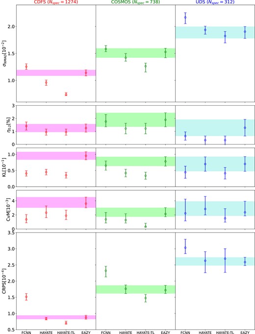
Visualization of the comparison in the photo-z and PDF statistics between different models presented in Table 2. The results for CDFS, COSMOS, and UDS are provided in the left, middle, and right columns, respectively. Each row shows evaluation scores of one metric for the baseline FCNN, hayate, hayate-TL, and eazy. The shaded region in each panel represents the 1σ range of the individual metric obtained from eazy for a given field; the error bars are 1σ.
Sections 5.1 and 5.2 describe the performance of hayate and hayate-TL. In Section 5.3, we discuss the benefit of our simulation-based CNN method, which outperforms the other ML approaches. Section 5.4 presents example archetypes of photo-z outliers useful in exploring the limitations of, and potential improvements to hayate when dealing with catastrophic errors in photo-z estimation.
5.1 hayate versus eazy
5.1.1 Photo-z statistics
Table 2 compares the performance of hayate with eazy. We see that hayate’s point estimates are comparable to, or better than, eazy, with σNMAD significantly reduced from 1.14 to 0.96 and 1.53 to 1.42 for CDFS and COSMOS, respectively. Probing the distribution of the test data on a zspec − Δz plane further provides insights into how accurate photo-z’s can be attained. The upper row in Fig. 7 shows the results for CDFS, where the photo-z’s derived with hayate (zhayate) and eazy (zeazy) are plotted on the left and middle panels, respectively. Figs A1 and A2 also present the outcomes for COSMOS and UDS (Appendix A) in the same manner. We can see from these figures that the distribution of errors between the two methods are comparable.
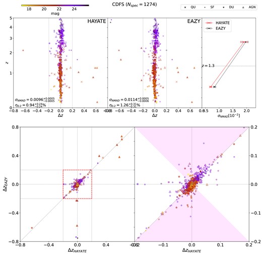
Top: distributions of the spec-z catalogue sample for CDFS on the zspec − Δz plane, which are obtained by testing hayate (left) and eazy (middle). Each data point is presented in different markers and colours, which represent the galaxy type and Ks-band magnitude. The threshold of Δz outliers is set to 0.2, which is shown by the vertical lines, and the outliers are represented by the filled markers. The right panel presents the comparison of σNMAD between low-z (z < 1.3) and high-z (z > 1.3) samples, individually derived with hayate and eazy. Bottom: comparison of photo-z errors (|Zph − Zsp|) between hayate (Δzhayate) and eazy (Δzeazy) for the same sample presented in the top panel. Each panel contains residual plots of the individual objects, whose entire distribution is presented in the left panel, while the zoom-in plot within the outlier threshold of |Δz| = 0.2 is in the right panel. The shaded region represents the area where zhayate is better than zeazy.
We also compare the residuals of hayate and eazy and see a strong correlation. The bottom row of each figure shows plots of Δzeazy versus Δzhayate for the test spec-z sample, which represent photo-z errors for eazy and hayate expressed as Δzeazy = (zeazy − zspec)/(1 + zspec) and Δzhayate = (zhayate − zspec)/(1 + zspec). The data points are generally aligned along the diagonal identity line, which demonstrates the ability of hayate to reproduce photo-z estimates that could be provided by eazy. The trained network replicates the high accuracy of the template-fitting code but with an execution time ∼100 times faster. This indicates hayate can learn to function as a reliable and efficient emulator of eazy. The resulting mock data should thus coincide with likely eazy template fits of the corresponding observed data.
The results for CDFS and COSMOS show slight improvements in photo-z point estimates with σNMAD reduced by 16 per cent and 7 per cent, respectively. The right panel of each upper row in Fig. 7, and Figs A1 and A2 shows this is mainly attributable to low-z galaxies, which presents σNMAD separately for subsamples obtained by splitting the test set with a redshift threshold of zspec = 1.3. This can be expected, since the underlying SED templates used for training are constructed with reliable low-z data. The interpolative nature of ML approaches further surpasses the one-on-one matching of the original template fitting by circumventing the individual template mismatch.
Another significant benefit of our ML method is the ability to generalize to galaxies at higher redshifts in the absence of a large body of high-z data. The photo-z precision obtained with hayate shows no significant difference from that with eazy even in the extrapolated high-z regime 1.3 < zspec < 5. The extensibility of the target redshift range ensures that the simulations are sufficiently effective beyond the training domain of firm underlying knowledge.
Applying ML approaches to the template fitting algorithm also produces a more robust photo-z estimator than eazy. The outlier rate η0.2 of estimated photo-z’s significantly drops from 1.26 per cent to 0.94 per cent, 1.90 per cent to 1.22 per cent, and 1.28 per cent to 0.32 per cent for CDFS, COSMOS, and UDS, respectively, as shown in Table 2. hayate is therefore less prone to catastrophic failures in photo-z predictions, performing well on 14 test sources whose photo-z errors would be outliers if derived with eazy. We classify them as Class A, along with other sample groups defined based on a set of Δzhayate and Δzeazy for each galaxy as presented in Table 3. Class B, on the other hand, only contains two galaxies, which are photo-z outliers for hayate but not for eazy.
Classification of the test objects based on their photo-z’s estimated with hayate and eazy. Objects of Class A are photo-z outliers for eazy whose estimates are significantly improved with our ML method so that they are no longer outliers for hayate. Class B contains a few galaxies on which eazy conversely outperforms, while photo-z outliers for both models are classified into Class C. Class D includes ‘normal’ galaxies whose photo-z’s provided by both models are not catastrophically wrong with respect to the spec-z’s.
| Object class | Description | Definition | Number of objects | ||
|---|---|---|---|---|---|
| CDFS | COSMOS | UDS | |||
| Class A | Photo-z outliers only for eazy | |Δzhayate| < 0.2, |Δzeazy| ≥ 0.2 | 5 | 6 | 3 |
| Class B | Photo-z outliers only for hayate | |Δzhayate| ≥ 0.2, |Δzeazy| < 0.2 | 0 | 1 | 0 |
| Class C | Photo-z outliers both for hayate and eazy | |Δzhayate| ≥ 0.2, |Δzeazy| ≥ 0.2 | 11 | 8 | 1 |
| Class D | Plausible photo-z estimates | |Δzhayate| < 0.2, |ΔzeazY| < 0.2 | 1257 | 723 | 308 |
20 catalogue objects classified as Class C in Table 3 show catastrophic solutions for photo-z computation with both models. Their wrong photo-z estimates are, however, quite similar between the two different methods, which are plotted on the diagonal in each bottom panel of Fig. 7, and Figs A1 and A2. From visual inspection, they are obviously not well represented by the SED template set of eazy, which indeed includes some rare objects such as 10 active galactic nuclei (AGNs) and 3 dusty star-forming galaxies. Improving photo-z estimations for Class C objects thus requires extending the population of galaxy templates used by eazy and for simulating our high-redshift sources. Brescia et al. (2019) also note that to increase the accuracy of AGN photo-z’s with template-fitting methods, the inclusion of morphological information (extended or point-like) likely provides the biggest improvement. Example plots of inputs and outputs for these sources are shown in Fig. 11, which are further discussed in Section 5.4.
5.1.2 PDF statistics
The quality of output PDFs is generally improved with our ML method as measured by KL, CvM, and CRPS, detailed in Table 2 and shown in Fig. 6. hayate particularly shows better PIT distributions for CDFS and COSMOS, with KL and CvM significantly lower than those derived with eazy. Fig. 8 presents the PIT histograms of hayate and eazy for these two fields, along with their CDFs used for quantifying deviations from uniformity. KL provides a dissimilarity measure between the predictive and uniform distributions of PIT, while CvM is a CDF-based metric intuitively represented by the area filled between the corresponding CDF and the identity line. We can see that the PIT distribution of hayate looks flatter than that of eazy, which is reflected by the smaller KL and CvM, indicative of better-calibrated PDFs.

PDFs of PIT distributions and their CDFs for the test catalogue samples in CDFS (left) and COSMOS (right). The PIT distributions derived with hayate and eazy are shown in the coloured and grey bar charts, respectively. The corresponding CDFs are given by the solid lines in the same colours. The dotted horizontal and diagonal lines represent the uniform PDF and the corresponding identity CDF, respectively, indicative of the perfectly calibrated distribution.
A major contributor to this is the application of ensemble learning to generating the combined PDFs. Fig. 9 shows the metrics estimated for different numbers of CNNs whose individual predictions are combined into the ensemble PDF. The single network is trained on the whole training sample, while the multiple models are built with ensemble learning, as discussed in Section 4.7. Increasing the number of networks remarkably improves KL and CvM, which converges as the number of individual PDFs increases to ∼15. Our fiducial configuration therefore uses 15 networks, as depicted by the vertical line in each panel. ML photo-z codes typically provide PIT distribution characteristics of convex shape, indicative of overly broad PDFs that are unlikely to include spec-z’s in their tails (Schmidt et al. 2020). The broadening of PDFs suggests an intrinsic function of ML training approaches that adds implicit smoothing to the effective error scale (Wolf 2009). Conversely, hayate produces redshift PDFs whose PIT distribution is rather similar to that obtained with the template-fitting code eazy, as one can see in Fig. 8. An over-representation of extreme values is evidenced by a concave histogram, implying overly narrow PDFs. The ensemble learning technique is aimed at alleviating this tendency by combining multiple predictions.

Changes in photo-z and PDF metrics with the number of CNNs whose predictions are combined into an ensemble. Each lower-level network is trained on a bootstrapped subsample for a given noise realization. The fiducial configuration of hayate incorporates 15 components, which is shown by the vertical dotted lines. The results for CDFS, COSMOS, and UDS are provided in red, green, and blue, respectively, while the shaded regions represent the 1σ ranges of the corresponding metrics estimated for eazy. The leftmost column presents the result for a single CNN that is trained on the entire training sample, while the last column shows the metrics obtained from the model purely trained with the CCE loss function without CRPS loss contribution.
Eriksen et al. (2020) have demonstrated a similar effect whereby combining multiple networks reduces the number of objects with the lowest and highest PIT values. The improvement in PIT distribution proved to be caused by decreasing photo-z outliers. However, this does not apply to hayate, since the outlier rate does not significantly drop with multiple PDFs combined. Our ensemble approach samples the potential solution space from different local minima on the loss surface.
We assess the overall form of PIT distributions to probe if the output PDFs are well calibrated on average. This requires that the CDF value at the spec-z should be random, rather than that each PDF is well constrained with respect to its true redshift. The quality of the individual PDFs thus has to be assessed in conjunction with CRPS, which represents a distance between the CDF of a given PDF and a step function with a step at its spec-z. In a derivative form, this can be translated into how different the PDF is from the corresponding delta function. We none the less often find a trade-off between KL/CvM and CRPS, or the uniformity of the PIT distribution and the sharpness of each PDF. A simple explanation for this is that a narrower PDF tends to be better constrained at its spec-z with lower CRPS, which is more likely to increase the number of PIT values at extreme edges.
We see in Fig. 9 that ensemble learning also improves CRPS slightly as the number of networks increases. At convergence, hayate’s PDF statistics are each comparable to, or better than, eazy. The validity of each output PDF is further supported by the sufficiently small CRPS. In Fig. 9, we see that the primary contribution to this is incorporating the CRPS term into the joint loss function. The results for the model trained exclusively with the CCE loss are presented on the rightmost columns in each panel. The inclusion of CRPS in the training loss function remarkably decreases the CRPS of output PDFs.
The analysis on the PDF statistics indicates the output PDFs derived with hayate are more reliable than those obtained with eazy, with respect to spec-z’s, while their overall population is statistically more self-consistent. We thus demonstrate hayate attains good-quality photo-z PDFs by leveraging the benefits of multiple approaches, which performs as an ensemble of lower-level networks optimized for the joint loss.
5.2 Improvements with transfer learning
Fig. 6 also demonstrates further improvements in photo-z precision due to transfer learning. The hayate-TL model shows an improved precision for all fields, with reduction in σNMAD by 30 per cent (CDFS), 13 per cent (COSMOS), and 7 per cent (UDS), respectively. By leveraging empirical data, hayate-TL achieves more accurate photo-z estimates than hayate and eazy with no more than ≲ 1000 additional observational training examples. The enhancement of the model’s performance none the less correlates with the sample size of spec-z data available. Accomplishing better performance with transfer learning is likely with a larger sample size.
The higher precision of photo-z point estimates indeed results from improved output PDFs yielded by hayate-TL. Table 2 shows significantly better CRPS for CDFS and COSMOS, which reduces from 0.83 to 0.70 and 1.76 to 1.48 with the assistance of spec-z information for re-training. The fine-tuning of the pre-trained network thus better constrains each redshift PDF over the peak around the spec-z. The improved PDF consequently provides a more precise photo-z point estimate.
The hayate-TL photo-z outliers still comprise exactly the same objects as hayate. The outlier rate consequently remains the same despite the re-training with observations. This reflects the limitation of transfer learning from simulations, which exclusively benefits an ‘ordinary’ test object whose colour–redshift relation can be fine-tuned by training with the remaining sample. It can not adapt to ‘anomalous’ sources whose photometric data are not sufficiently represented in the training set along with reliable spec-z’s. We therefore conclude the photo-z outliers found with hayate are intrinsically inconsistent with the input–output mapping derived from both the template-based training set and the observed data.
Table 2 also presents the result for the CNN model which is trained on the same spec-z samples as used for transfer learning but completely from scratch. hayate-TL significantly outperforms the most common method of training purely with spec-z data, although both fundamentally learn with the same observed samples. Training with simulations proves to supplement the insufficient spec-z sample for training. These results indicate transfer learning is effective for making a minor adjustment both for output redshift PDFs and their single-point estimates using spec-z information. Training with simulations lays important groundwork for the subsequent observational fine-tuning.
5.3 CNN versus FCNN
Evaluating the metrics for the two ML models, the baseline FCNN and hayate, reveals the CNN-based architecture shows overall improvements on photo-z point estimates. Table 2 and Fig. 6 show significant drops in σNMAD, η0.2, and CRPS for all the fields. This indicates that the CNN is more likely to yield reliable redshift PDFs with precise point estimates than a FCNN.
The superior performance of hayate compared to the FCNN model indicates the benefit of prioritizing local feature extraction from the combined arrays of fluxes and photometric errors. CNNs are particularly suited to high-dimensional data such as image processing since convolutional kernels require many fewer trainable parameters than FCNNs. Convolution operations are performed primarily for extracting local information and preserving the spatial relationship between features; these features become more abstract from layer to layer through the network. The CNN photo-z models have commonly been trained on galaxy images instead of photometry summary information, which allows for learning with Supporting Information on the spatial flux distribution (Pasquet et al. 2019; Schuldt et al. 2021; Henghes et al. 2022; Lin et al. 2022; Zhou et al. 2022). Our ML instead leverages the demonstrated ability of CNNs to capture and interpret the local features of galaxy SEDs obtained from the flux distribution over a range of wavelengths.
5.4 Analysis of individual redshift PDFs
The robustness of our method can be explored with by visual inspection of individual PDFs predicted by hayate and eazy. We particularly focus on the test objects classified as Class A, defined in Table 3, which are responsible for the improved outlier rate versus template-fitting approaches. Fig. 10 shows example star-forming galaxies of Class A, whose input photometric data and output PDFs are presented in the top and bottom rows of each panel, respectively. hayate obviously performs better than eazy on these objects, providing more reliable PDFs with respect to their spec-z’s, which are represented by the black circles on the horizontal axes. This results in more accurate photo-z point estimates than the eazy predictions, shown by the coloured and grey vertical lines.

Example star-forming galaxies of Class A. The input fluxes with errors are plotted in the top row of each panel, along with the missing values represented by the black crosses. The grey dotted line shows the best-fitting SEDs optimized with the photo-z by eazy (zeazy), while the coloured solid line represents the result at the fixed photo-z derived with hayate (zhayate). The bottom row compares the photo-z PDFs produced by hayate and eazy, shown by the shaded region and the solid black line, respectively. For each object their photo-z point estimates are given by the coloured and grey upside-down triangles, while the spec-z by the down arrow.
We can gain further insight into the reason for the improvements by probing the best-fitting SEDs derived with eazy when fixed to the photo-z’s. They are represented by the coloured lines plotted with the input fluxes, which can be compared to the grey dotted lines for the corresponding SEDs of eazy photo-z’s. One major failure of template fitting is to misinterpret the spectral features of the Lyman and Balmer breaks, or the Lyman-alpha and Balmer emission lines (Benítez 2000; Brammer et al. 2008). Some of the PDFs produced by hayate indeed show minor peaks around their corresponding eazy photo-z’s, showing the learned degeneracy inherited from the original template-fitting algorithm.
We may glean further clues for improving hayate’s output PDFs by investigating typical photo-z outliers, although the outlier rate is low with |$\eta _{0.2}\lesssim 1~{{\ \rm per\ cent}}$|. One major group consists of rare objects whose photometric data are not well represented by the training samples. We can see some likely AGN data points (estimated from visual inspection of spectra) in the lower left panels of Fig. 7 and Fig. A1, depicted by triangles outside the region of |Δzhayate| < 0.2 and |Δzeazy| < 0.2. These objects are included in Class C, whose photo-z’s are outliers both for hayate and eazy often with similar point estimates. For the example AGNs presented in Fig. 11, both models provide PDFs of erroneous photo-z’s, although their input photometric data are obtained with the brightest magnitudes and the highest signal-to-noise ratios (SNRs). Most of them show no minor peaks at the spec-z’s in the distributions. This reveals the ensemble of standard eazy templates can not intrinsically cover galaxy SEDs of some rare objects, which means that the simulated training data sets will also lack objects of this class, and such anomalous objects result in catastrophically wrong solutions.

Example AGNs of Class C in CDFS and COSMOS.
Class C also contains some star-forming galaxies which result in incorrect photo-z predictions. They are varied in photometric SNR and derived spec-z’s, whose results are presented in Fig. 12. hayate and eazy both predict quite similar photo-z’s for each object, although they are significantly divergent from the spec-z. One can find the best-fitting SEDs derived at zhayate and zeazy which indeed look well fitted to the input fluxes. A deficiency in the template set and thus hayate’s training data means that neither can correctly classify these difficult objects.

Example star-forming galaxies of Class C.
Photo-z point estimates of hayate are generally correlated with those computed by eazy, as discussed in Section 5.1.1. The network is clearly able to exploit the demonstrated ability of template fitting to predict precise photo-z’s. Assessing the model’s performance on the individual outliers further demonstrates how our hybrid approach has internalized the fundamental functions of eazy, including even the failure to produce reliable PDFs for some difficult objects. One remarkable benefit of hayate is, however, the potential to remedy the vulnerability of eazy to the misinterpretation of spectral features, particularly characterized by the Lyman and Balmer breaks.
6 DISCUSSION
We have demonstrated the potential for hayate to contribute to efficient data mining for future large surveys with the following benefits:
Our method can be applied to a broad redshift range including high-z galaxies which are deficient in reliable observational data for training. The network trained with template SEDs from eazy can function as a reliable emulator, with ∼100 times shorter running time.
The analysis of σNMAD reveals that in the interpolative regions of the low-z colour space, the ML methodology results in higher accuracy in photo-z estimation than the original template-fitting approach. It also performs comparably well even in the high-z extrapolative regime.
hayate is likewise more robust to photo-z outliers than eazy. In particular, its output photo-z PDFs are less vulnerable to the degeneracy of redshift caused by misinterpretation of the Lyman and Balmer breaks from input photometric data.
Optimizing the joint loss comprising LCCE and LCRPS keeps the credibility of individual PDFs comparable to that for eazy in terms of CRPS.
Ensemble learning shows significant improvements in KL and CvM, which enables hayate to provide redshift PDFs better calibrated than eazy with a flatter PIT distribution.
Transfer learning with hayate-TL significantly improves the model’s performance further, achieving more reliable photo-z point estimates and PDFs than hayate. This reduces σNMAD by |$\sim 5\,\mathrm{ per}\,\mathrm{ cent}-30~{{\ \rm per\ cent}}$| depending on the sample size of spec-z data sets. We expect to benefit from the fine-tuning with spec-z information for future photo-z studies, since spectroscopy will be conducted along with imaging in many upcoming survey projects.
Training with simulations shows remarkable improvements in both photo-z and PDF statistics compared to the purely observation-based training. This enables us to utilize ML techniques for redshift estimations where only small spec-z samples are available: in this work, no more than 1274, 738, and 312 objects in CDFS, COSMOS, and UDS, respectively.
Our empirical noise application method allows any missing values to be included in the input photometric data. This can enhances photometric resolution and spectral coverage of the target photometric sample without reducing sample size, which is compiled from multiple subcatalogues by cross-matching between individual sources of different many-band photometry.
It is worth pointing out that, although a hybrid method optimized to perform well in the high-redshift regime, there is no clear step-change in performance beyond a certain threshold. hayate performs well across the entire parameter range, exploiting the strengths of the two approaches previously considered somewhat disjoint.
Exploring billions of objects catalogued by the Stage IV DESs will require the exploitation of photo-z’s at the expense of reliable spec-z information. A simplistic extrapolation from past campaigns would estimate over 10 000 yr of continuous integration time for obtaining spectra of the LSST ‘gold sample’ galaxies (Newman & Gruen 2022). We may need ≳ 30 000 spectra in training and calibration of photo-z’s for a Stage IV survey, from ≳ 15 widely separated fields of ∼0.09 deg2 each; for instance, this corresponds to an estimated survey time of over a few years even with the Extremely Large Telescope for the LSST survey depths (Newman et al. 2015). The limited redshift range targeted by the Euclid survey could rather demand a smaller spec-z sample size to meet the cosmology requirements for photo-z calibration, but still exceeding ∼5000 (Stanford et al. 2021). Efficient and accurate estimation of photo-z’s will have fundamental importance in various fields of extragalactic astronomy and cosmology as the pace of follow-up spectroscopy is never able to sufficiently meet the required volume of objects from such imaging surveys.
Template-fitting methods perform well on the current generation of surveys, though at the data volumes of the levels expected for the Stage III and IV surveys the compute power needed becomes a non-trivial issue. A photo-z estimator that is orders of magnitude faster while preserving excellent performance would assist in scaling these data pipelines.
This work builds on the performance of eazy, applied to S16 (including the data products from the ZFOURGE survey), which covers 128 arcmin2 to a limit of AB ∼ 26 in the Ks band for CDFS, producing imaging of ∼30 000 galaxies. The ongoing and future surveys will probe much fainter objects in wider survey areas, producing observational catalogues of unprecedentedly large sample size.
Our hybrid method can be applied to any photometric catalogues by simulating photometry using the corresponding transmission curves for mock SEDs with simulated noise based on the observational errors. The simulation-based catalogue construction also allows training methods to be extrapolated outside their initial redshift ranges, that is, z < 1.3 in this work. We set the upper bound of the target redshift range to 5 considering the number of spec-z data available as the test samples. This can be reasonably extended to much higher redshifts depending on the target survey or photometric catalogue. Some recent works have proposed using simulated photometric data in training photo-z networks (e.g. Eriksen et al. 2020; Ramachandra et al. 2022), but the redshift range still covers up to ∼1.2 at the highest.
The mainstream in traditional ML approaches have involved training a photo-z algorithm exclusively with spec-z information (e.g. Firth, Lahav & Somerville 2003; Brescia et al. 2013, 2014; Bonnett 2015; Sadeh et al. 2016; Jones & Singal 2017). The accuracy of predicted photo-z’ s essentially depends on the quality and completeness of the training data set, which requires large spec-z samples. The target redshift range for ML has been thus limited to low-z regions of sufficient spectroscopic completeness. This accounts for the current prevalence of template-based methods for high-z galaxies, although ML approaches are rather common at z ≲ 1. The extensibility of the target redshift range is one critical functionality of our hybrid method that will enable to infer accurate photo-z’s of faint high-z galaxies obtained from the upcoming survey projects.
We have also demonstrated the potential of transfer learning to fine-tune the pre-trained model with spec-z information and improve the photo-z precision of normal sources, whose estimations are not outliers with respect to Δz. This will significantly benefit future ML photo-z studies, since spectroscopy will be conducted along with imaging in many upcoming survey projects.
Forthcoming programs from the JWST will provide opportunities to both improve the algorithm and to put it into practice. Deep spectroscopic data will bolster the training set available for transfer learning. For instance, the ongoing JWST Guaranteed Time Observations (GTO) program, the JWST Advanced Extragalactic Survey (JADES; Bunker, NIRSPEC Instrument Science Team & JAESs Collaboration 2020; Rieke 2020) will provide Near InfraRed Spectrograph (NIRSpec) spectroscopy covering in ‘DEEP’ survey mode a smaller survey area of 46 arcmin2 in the Hubble Ultra-Deep Field (HUDF) Great Observatories Origins Deep Survey (GOODS) South but to a much fainter limit of AB ∼ 30. Another survey mode, the ‘MEDIUM’ survey, will cover no less than 190 arcmin2 in GOODS-S and GOODS-N to a limit of AB ∼ 29. JADES will observe ∼5000 galaxies at 1 < z < 5, ∼2000–4000 galaxies at z > 5 and ∼300 galaxies at z > 6.
On the other hand, deep imaging surveys, such as Public Release IMaging for Extragalactic Research (PRIMER, Dunlop et al. 2021) will probe an even larger area of ∼400 arcmin2 than GTO in COSMOS and UDS to a limit of AB ∼ 28.5, revealing ∼100–200 K galaxies out to z ∼ 12. The COSMOS-Webb (Kartaltepe et al. 2021) will also produce wide area imaging covering 0.6 deg2 in COSMOS to a limit of AB ∼ 28, expected to offer near-IR imaging of half a million galaxies along with 32 000 in the mid-IR and identify hundreds of massive quiescent galaxies in the first 2 Gyr (z > 4). These imaging data sets will be excellent candidates for applying hayate, and via transfer learning will leverage the smaller spectroscopic surveys.
The non-Gaussianity of predicted PDFs also distinguishes hayate from other commonly used approaches, which tend to assume the underlying components to be Gaussian (D’Isanto & Polsterer 2018; Eriksen et al. 2020; Lima et al. 2022). hayate yields non-parametric PDFs as the outputs of the softmax activation. Realistic redshift PDFs should indeed contain non-Gaussian properties such as asymmetry and tails, reflecting an interplay of various features in target photometric data: for instance, filter functions, the set of filters used and their observational error distributions. They may also be vulnerable to colour–redshift degeneracies, which are represented by multiple peaks. These individual features could have a significant impact on cosmological measurements (Mandelbaum et al. 2008; Palmese et al. 2020).
Nevertheless, hayate still fails to return a uniform PIT distribution, required for applying the the output PDFs to estimating N(z) of an ensemble of galaxies (Newman & Gruen 2022). eazy is not vulnerable to systematic broadening or narrowing of output PDFs in general (Wittman, Bhaskar & Tobin 2016; Schmidt et al. 2020). The better calibration of redshift PDFs offered by hayate thus provides insight into obtaining an even flatter PIT distribution that could meet the requirements for many high-precision cosmology measurements. Improving the ensemble learning approach, combined with transfer learning depending on the science case, is an potential avenue of research, which has contributed to significantly reducing KL and CvM.
Another issue to be addressed is the fidelity of simulated training data. The success of transfer learning indicates that there remains an intrinsic disparity in data quality between simulated and observed data sets, and that the mock photometric data used for training can be further improved. In essence, the quality of the mock SEDs relies on the performance of eazy, while the noise model affects simulated photometry for a given test sample. These aspects of our hybrid method simultaneously lead to hayate’s ability to emulate eazy and its limitations, while surpassing the performance of the original template-fitting code.
7 CONCLUSION
We have developed a novel photo-z CNN, dubbed hayate, based on a hybrid method that incorporates the demonstrated ability of template fitting into the latest empirical modelling. It is primarily aimed at combing the benefits of ML- and template-based approaches by performing as an efficient ML emulator of eazy beyond the limitations of spec-z completeness at low-z. This was achieved by extrapolating the SED coverage obtained from low-z photometric data to higher redshifts. Technically, we artificially redshifted eazy best-fitting SEDs for the S16 sources of z < 1.3 such that the training set of mock SEDs covers a broader redshift range up to z = 5. Further advancements were likewise explored via simultaneous optimization of output photo-z PDFs and point estimates, aided by the modern ML techniques: training with the joint loss function (Section 4.5), ensemble learning (Section 4.7), and transfer learning (Section 4.6). The photo-z networks of different configurations, as well as eazy, were tested on the updated S16 spec-z samples, evaluated based on commonly used performance metrics for measuring the quality of photo-z point estimates and output PDFs: σNMAD, η0.2, KL, CvM, and CRPS, as described in Section 4.4.
Considering the applicability of our methodology to a variety of catalogues, hayate should generalize to a flexible set of photometric bands. The current framework is a bespoke solution for a specific catalogue with a fixed combination of broad-band filters. We may develop an extended architecture where the input involves a broader range of photometric band filters by allowing missing data to be incorporated into those unavailable to a given catalogue. A single model could then adapt to different catalogues simultaneously by learning on a collection of individual training samples. An upgraded model is under development and will be the subject of a future work.
Further improvements require a strategy to extend the training sample beyond the scope of eazy predictions. The simplest approach would be to incorporate a broader range of galaxy SEDs from external sources into the training set, enhancing the model’s robustness to those photo-z outliers whose typical SEDs are not included in the eazy outputs. This particularly applies to some of the example galaxies discussed in Section 5.4 including AGNs.
Blended spectra are a likely source of photo-z errors, and difficult to eliminate in the pre-processing stage. All photo-z methodologies are vulnerable to this source of contamination, for which a correct redshift is not defined. It is possible that future methods, such as ML-based algorithms which directly consume the 2D spectra, could mitigate this further.
Our hybrid method may both benefit from and complement other recent developments. Wang et al. (2023b) have demonstrated promising results by using carefully chosen priors to break the age–mass–redshift degeneracy, and have recovered accurate photo-z's using the Prospector–α (Leja et al. 2017) stellar population properties inference code, simultaneously recovering redshift with other stellar properties using Bayesian inference. Wang et al. (2023a) exploit simulation-based inference (SBI; Cranmer, Brehmer & Louppe 2020), which allows efficient sampling of computationally expensive models, to massively accelerate this multiparameter fitting compared to nested sampling by up to a factor of 104. These methods, applied to simulated JWST data, efficiently recovered photo-z's with comparable outlier rates (σNMAD ∼ 0.04) along with multimodal PDFs.
ACKNOWLEDGEMENTS
KG and CJ acknowledge support from Australian Research Council Laureate Fellowship FL180100060. Part of this work was performed on the OzSTAR facility at Swinburne University of Technology.
DATA AVAILABILITY
The data sets were derived from sources in the public domain at https://zfourge.tamu.edu.
References
APPENDIX A: RESULTS FOR COSMOS AND UDS

The same figure as Fig. 7, but for COSMOS.
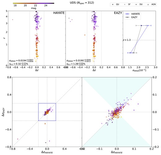
The same figure as Fig. 7, but for UDS.
APPENDIX B: SUMMARY OF PHOTO-Z FCNNS IN THE LITERATURE
Summary of major FCNN models developed in the previous photo-z studies which were trained with spec-z information.
| Reference | Architecturea | Target sampleb | Photometric informationc | |||
|---|---|---|---|---|---|---|
| Spec-z data | Sample size | Redshift range | Survey | Filter band | ||
| 1 | {Ninput = 5: | SDSS-EDR | ∼7000 | zspec < 0.5 | SDSS-EDR | ugriz |
| 6 × 3: 1} | ||||||
| 2 | {Ninput = 5: | SDSS-EDR | ∼10 000 | zmed = 0.104 | SDSS-EDR | ugriz |
| 10: 10: 1} | ||||||
| 3 | {Ninput = 7: | AGES | 5052 | zspec ≲ 1.0 | NDWFS-DR3 | BWRI |
| 10 × 3: 1} | zAGN ≲ 3.0 | IRAC Shallow Survey | [3.6][4.5][5.8][8.0] | |||
| 4 | {Ninput = 43: | SDSS-DR9 | 347 342 | zspec ≲ 1.0 | SDSS-DR9 | ugriz |
| 2Ninput + 1: | GALEX | nuv, fuv | ||||
| Ninput − 1: 1} | UKIDSS | YJHK | ||||
| WISE | W1, W2, W3, W4 | |||||
| 5 | {Ninput = 5: | VVDS | 22 072 | zspec ≲ 1.4 | CFHTLenS | u*g′r′i′z′ |
| 12: 12: PDF}d | VVDS-F22 | |||||
| DEEP-2 | ||||||
| VIPERS | ||||||
| 6 | {Ninput = 5: | SDSS-DR10 | ∼180 000 | zspec ≲ 0.8 | SDSS-DR10 | ugriz |
| Ninput + 1: | ||||||
| Ninput + 9: | ||||||
| Ninput + 4: 1} | ||||||
| 7 | {Ninput = 74: | SDSS-DR15 | 159 074 | zspec ≲ 2.0 | SDSS-DR15 | ugriz |
| 528: PDF} | zQSO ≲ 7.0 | WISE | W1W2 | |||
| 8 | {Ninput = 4: | 15 spec-z | ∼150 000 | zspec ≲ 1.0 | Pan-STARRS1-DR1 | grizy |
| 128: 256: | catalogues | |||||
| 512: 1024: | (e.g. SDSS-DR15 | |||||
| 512: 256: | LAMOST-DR5 | |||||
| 128: 32: PDF} | 6dFGS | |||||
| PRIMUS) | ||||||
Notes. References: (1) Firth et al. (2003); (2) Collister & Lahav (2004, ANNz1); (3) Brodwin et al. (2006); (4) Brescia et al. (2013, 2014, MLPQNA); (5) Rau et al. (2015); (6) Sadeh et al. (2016, ANNz2); (7) Ansari, Agnello & Gall (2021); and (8) Lee & Shin (2021).
a Each architecture is denoted by {Ninput: N1: Nhidden × n:...: Noutput}, where Ninput and Noutput are the numbers of input and output nodes respectively, while the first hidden layer contains N1 neurons, followed by a sequence of n hidden layers with Nhidden neurons each, which is represented by Nhidden × n.
b Spec-z sample used for evaluating the performance of a photo-z network. All the models can provide each target object with a photo-z point estimate, either as immediate output or from an output PDF of redshift. Spec-z data from different surveys can be incorporated into a collection of multiple catalogues depending on the individual work.
c Photometric data used as input. The target spec-z sample is basically limited to objects that have photometric data for all the filter bands presented in the rightmost column.
dNoutput = 1 implies that the model predicts a photo-z point estimate for each object, while Noutput = PDF it produces a PDF of redshift as immediate output.
Summary of photo-z FCNN models which were trained with simulations.
| Reference | Architecture | Target sample | Photometric information | |||
|---|---|---|---|---|---|---|
| Spec-z data | Sample size | Redshift range | Survey | Filter band | ||
| 1 | {Ninput = 7: | SDSS-DR1 | 88 108 | zspec ≲ 0.4 | SDSS-DR1 | ugriz |
| 12: 10: 1} | ||||||
| 2 | {Ninput = 46: | zCOSMOS-DR3 | 8566 | zspec ≲ 1.2 | PAUS | 40 narrow bands |
| 600: 400: | |$(4500-8500{{\mathring{\rm A}}})$| | |||||
| 250 × 13: PDF} | CFHTLenS | u* | ||||
| COSMOS-20 | BVri+z++ | |||||
| 3 | {Ninput = 5: | SDSS-DR15 | 1 965 800 | zspec ≲ 1.0 | SDSS-DR15 | ugriz |
| 512: 1024: | VIPERS | CFHTLS | ugriz | |||
| 2048: 1024: | DEEP-2 | |||||
| 512: 256: 128 | ||||||
| 64: 32: PDF} | ||||||
| 4 | {Ninput = 20: | Simulationa | ∼10 000 | zsim ≲ 4.0 | CSST | NUV, ugrizy |
| 2Ninput × 2: 1} | ||||||
| {Ninput = 20: | ||||||
| 2Ninput × 6: 1} | ||||||
| This | {Ninput = 76: | S16 | 1,273 | zspec < 5.0 | ZFOURGE | J1J2J3HsHlKs |
| work | 500 × 3: PDF} | (e.g. FORS2 | HUGS | KsHI | ||
| (CDFS) | K20 | TENIS | tenisK | |||
| VVDS | VIMOS | U, R | ||||
| CXO | ACS | BVIZ | ||||
| IMAGES | ESO DPS | U38VRc | ||||
| VIMOS) | 3D-HST | F140W, F814W | ||||
| Update on zspec data | WFC3 ERS | F098M, F125W, F160W | ||||
| (MOSDEF | CANDELS | F105M, F125W, F160W | ||||
| MOSEL | F606W, F814W | |||||
| VANDELS) | MUSYC | IA484, IA527, IA574 | ||||
| IA598, IA624, IA651 | ||||||
| IA679, IA738, IA767 | ||||||
| IA797, IA856 | ||||||
| IUDF | [3.6][4.5] | |||||
| GOODS | [5.8][8.0] | |||||
