


ABSTRACT
We present the first comprehensive halo occupation distribution (HOD) analysis of the Dark Energy Spectroscopic Instrument (DESI) One-Percent Survey luminous red galaxy (LRG) and Quasi Stellar Object (QSO) samples. We constrain the HOD of each sample and test possible HOD extensions by fitting the redshift-space galaxy 2-point correlation functions in 0.15 < r < 32 h−1 Mpc in a set of fiducial redshift bins. We use AbacusSummit cubic boxes at Planck 2018 cosmology as model templates and forward model galaxy clustering with the AbacusHOD package. We achieve good fits with a standard HOD model with velocity bias, and we find no evidence for galaxy assembly bias or satellite profile modulation at the current level of statistical uncertainty. For LRGs in 0.4 < z < 0.6, we infer a satellite fraction of |$f_\mathrm{sat} = 11\pm 1~{y{\ \mathrm{per\,cent}}}$|, a mean halo mass of |$\log _{10}\overline{M}_h/M_\odot =13.40^{+0.02}_{-0.02}$|, and a linear bias of |$b_\mathrm{lin} = 1.93_{-0.04}^{+0.06}$|. For LRGs in 0.6 < z < 0.8, we find |$f_\mathrm{sat}=14\pm 1~{{\ \mathrm{per\,cent}}}$|, |$\log _{10}\overline{M}_h/M_\odot =13.24^{+0.02}_{-0.02}$|, and |$b_\mathrm{lin}=2.08_{-0.03}^{+0.03}$|. For QSOs, we infer |$f_\mathrm{sat}=3^{+8}_{-2}\mathrm{per\,cent}$|, |$\log _{10}\overline{M}_h/M_\odot = 12.65^{+0.09}_{-0.04}$|, and |$b_\mathrm{lin} = 2.63_{-0.26}^{+0.37}$| in redshift range 0.8 < z < 2.1. Using these fits, we generate a large suite of high fidelity galaxy mocks, forming the basis of systematic tests for DESI Y1 cosmological analyses. We also study the redshift-evolution of the DESI LRG sample from z = 0.4 up to z = 1.1, revealling significant and interesting trends in mean halo mass, linear bias, and satellite fraction.
1 INTRODUCTION
Galaxies are biased tracers of the underlying matter density field of the Universe, and their distribution is an important source of cosmological and astrophysical information. However, while the distribution of dark matter is readily modelled by gravitational collapse, the distribution of galaxies is significantly more complex due to non-linear evolution and baryonic processes. Thus, to extract cosmology and galaxy physics from the observed galaxy distribution, it is critical to model the connection between galaxies and their underlying dark matter density field.
A key piece of simplification in galaxy–dark matter connection modelling comes in what is known as the halo model, where simulations have shown that galaxies form and evolve in dense dark matter clumps known as haloes (White & Rees 1978; Cooray & Sheth 2002). Within the halo model, we can empirically model the connection between galaxies and haloes through a set of probabilistic models known as the halo occupation distribution model (HOD; e.g. Peacock & Smith 2000; Scoccimarro et al. 2001; White, Hernquist & Springel 2001; Berlind & Weinberg 2002; Berlind et al. 2003; Zheng et al. 2005; Zheng, Coil & Zehavi 2007). The HOD formalism has been highly successful in characterizing magnitude-limited samples of bright galaxies in past galaxy redshift surveys (e.g. Zehavi et al. 2011; Parejko et al. 2013; Guo et al. 2014, 2015b; Rodríguez-Torres et al. 2016; Alam et al. 2020; Avila et al. 2020; Yuan et al. 2021b). HOD studies are important because they reveal aspects of galaxy evolution physics and test assumptions of galaxy–dark matter connection (e.g. Lange et al. 2019; Alam et al. 2020; Yuan et al. 2021a; Linke et al. 2022; Wang et al. 2022). They are also important in producing mocks that accurately reproduce the observed clustering and thus enable robustness tests of cosmology pipelines (e.g. Smith et al. 2020; Alam et al. 2021; Rossi et al. 2021). Most recently, simulation-based forward-modelling approaches have also utilized the flexibility of HODs to constrain cosmology from highly non-linear scales that are otherwise inaccessible with standard analytical approaches (e.g. Chapman et al. 2022; Kobayashi et al. 2022; Lange et al. 2022; Yuan et al. 2022a; Zhai et al. 2023).
The Dark Energy Spectroscopic Instrument (DESI) is a stage-IV spectroscopic galaxy survey with the primary goal of determining the nature of dark energy through the most precise measurement of the expansion history of the universe ever obtained (Levi et al. 2013; DESI Collaboration 2016). The baseline survey will obtain spectroscopic measurements of 40 million galaxies and quasars in a 14 000 deg2 footprint in 5 yr. This represents an order-of-magnitude improvement both in the volume surveyed and the number of galaxies measured over previous surveys. The DESI large-scale structure samples are divided into 4 target classes: the bright galaxy sample (BGS), the luminous red galaxies (LRG), the emission line galaxies (ELG), and the quasi-stellar objects (QSO). The auto- and cross-correlations of and between the four tracers probe the large-scale structure in increasing high redshift domains and combine to produce the most precise large-scale structure measurement from redshift z = 0.1 all the way to z = 2.1. Additionally, quasars that have redshifts greater than 2.1 are used as sightlines for Lyma α forest absorption, and the combination of ly α–ly α, ly α–QSO, and QSO–QSO correlations probe large-scale structure to z < 3.5.
The Early Data Release (EDR) of the DESI survey consists of data in the so-called One-Percent Survey, collected during the Survey Validation campaign (SV; DESI Collaboration 2024) before the start of the main survey operations. The One-Percent Survey covered 20 fields totalling 140 deg2 with final target selection algorithms similar to those of the main survey (Raichoor et al. 2020, 2023; Ruiz-Macias et al. 2020; Yèche et al. 2020; Zhou et al. 2020; Chaussidon et al. 2023; Hahn et al. 2023; Zhou et al. 2023). The one-per cent survey reaches higher completeness than the main survey and produces the first clustering measurements from DESI. Specifically, more than 95 per cent targets received fibers in the ELG sample, while more than 99 per cent of targets in each of the BGS, LRG, and QSO samples received fibers.
In this paper, we present a comprehensive HOD analysis of the DESI One-Percent Survey LRG and QSO samples. This paper is amongst a series of papers analysing galaxy–halo connection models with DESI One-Percent Survey data. This paper addresses the more well-understood samples of LRG and QSO, while the more novel ELG sample is analysed in a dedicated paper (Rocher et al. 2023). In parallel, there are also several Subhalo-abundance matching (SHAM) analyses. Specifically, Prada et al. (2023) provide an overview of the Uchuu-based SHAM analyses (Ishiyama et al. 2021). Yu et al. (2024) present SHAM analyses based on the unit simulation (Chuang et al. 2019). Beyond the single-tracer analyses, Gao et al. (2023) and Yuan et al. (2023) analyse the cross-correlation functions between the ELG and LRG tracers with multitracer SHAM and HOD models, respectively. These papers together present a significant variety of methodologies and mock products appropriate for a large scope of applications.
This paper is structured as the following. In Section 2, we introduce the observed samples and present their clustering measurements. In Sections 3 and 4, we introduce the simulation suite and the HOD models. In Section 6, we present LRG fits on both the projected clustering measurements and the full-shape redshift-space clustering measurements, and present the corresponding model constraints. We also present a first analysis of the redshift evolution of the DESI LRG sample and the physical implications. We present the QSO fits in Section 7. In Section 8, we present a series of mock products as a result of this analysis. Finally, we conclude in Section 9.
Throughout this paper, we adopt the Planck 2018 ΛCDM cosmology, specifically the mean estimates of the Planck TT,TE,EE+lowE + lensing likelihood chains: Ωch2 = 0.1200, Ωbh2 = 0.02237, σ8 = 0.811355, ns = 0.9649, h = 0.6736, w0 = −1, and wa = 0 (Planck Collaboration VI 2020).
2 DATA
In this section, we describe the LRG and QSO samples and present their respective clustering measurements.
DESI observed its One-Percent survey as the third and final phase of its Survey Validation program in April and May of 2021. Observation fields were chosen to be in twenty non-overlapping ‘rosettes’, where a high completeness was obtained by observing in each rosette at least 12 times (see DESI Collaboration (2024, b) for more details.
Prior to beginning SV, the DESI instrument (DESI Collaboration 2022) had proven its ability to simultaneously measure spectra at 5000 specific sky locations, with fibers placed accurately using robotic positioners populating the DESI focal plane (Silber et al. 2022). During SV, the DESI data and operations teams’ (Schlafly et al. 2023) proved their ability to efficiently process the spectra through the DESI spectroscopic pipeline (Guy et al. 2023). Thus, DESI was able to start from an initial target list (Myers et al. 2023) quickly obtain a highly complete One-Percent Survey.
The redshift measurements we use are available in the DESI EDR (DESI Collaboration 2023b).1 These were input to the large-scale structure (LSS) catalogues, also described in the EDR (DESI Collaboration 2023b). Briefly, these LSS catalogues apply quality cuts to the data samples and provide matched random catalogues that trace the angular footprint and dN/dz of the data, at a total density of 4.5|$\times 10^{4}$| deg−2. Lasker et al. (in preparation) describe how we compute the joint probabilities for a given set of targets to be observed by simulating 128 alternative realizations of the DESI One-Percent Survey fiber assignment. We use this information to determine the pairwise-inverse-probability (Bianchi & Verde 2020) weights to use in our clustering measurements to correct for the effect of fiber collisions. We further apply angular up-weighting (PIP + ANG; Bianchi & Verde 2020). Mohammad et al. (2020) showed that this weighting scheme provides an unbiased clustering down to |$0.1$|h−1 Mpc.
The One-Percent Survey LSS catalogues also include the so-called ‘FKP’ (Feldman, Kaiser & Peacock 1994) weights in order to properly weight each volume element with respect to how each sample’s number density changes with redshift,
where n(z) is the weighted number per volume, and P0 is a fiducial power-spectrum amplitude. We use P0 = 104 (h−1 Mpc)3 for LRG and P0 = 6 × 10³ (h−1Mpc)3 for QSO. For a detailed description of the weights and systematics treatment, we refer the readers to DESI Collaboration (2023b).
2.1 DESI One-Percent Survey LRG and QSO samples
The LRGs are an important type of galaxies for large-scale structure studies, and are specifically selected for observations due to two main advantages: (1) they are bright galaxies with the prominent 4000 Å break in their spectra, thus allowing for relatively easy target selection and redshift measurements; and (2) they are highly biased tracers of the large-scale structure, thus yielding a higher S/N per-object for the baryon acoustic oscillation (BAO) measurement compared to typical galaxies. The LRG sample is drawn from a parent photometric sample, where the SV target selection is defined in Zhou et al. (2020). The sample has a target density of 605 deg−2 in 0.4 < z < 0.8, significantly higher than previous LRG surveys (BOSS and eBOSS; Dawson et al. 2013, 2016), while the sample also extends to z ∼ 1. Within EDR, the LRG main sample consists of 89 059 galaxies, 43 269 in the northern footprint and 45 790 in the southern footprint.
Quasi-stellar objects (a.k.a. Quasars, or QSOs) are the tracers of choice to study large-scale structures at high redshift due to the fact that they are some of the most luminous extragalactic sources. DESI aims to obtain spectra of nearly three million quasars, reaching limiting magnitudes r ∼ 23 and an average density of ∼310 targets per deg2. Within EDR, the QSO selection yields 24 182 quasars within redshift range 0.8 < z < 2.1, and an additional 11 603 Ly α quasars at higher redshift. For this study, we focus on the quasars at z < 2.1 which will be used for quasar clustering analysis.
Fig. 1 shows the DESI One-Percent Survey LRG and QSO mean density as a funtion of redshift n(z). The vertical dashed lines correspond to fiducial bin edges defined for DESI cosmology studies. For the LRG sample, the number density remains fairly constant from z = 0.4 to z = 0.8 at approximately 5 × 10⁻⁴ h3 Mpc−3. At z > 0.8, the LRG density drops off quickly, suggesting increasing incompleteness and strong redshift evolution. To clarify, the redshift evolution in the selected LRG sample is likely mostly due to the specific colour selection used in DESI instead of evolution in the underlying sample. For the fiducial HOD analysis presented in Section 6, we examine the sample in two redshift bins: 0.4 < z < 0.6 and 0.6 < z < 0.8. These two bins are designated as the sample for DESI Y1 cosmology analyses, thus it is important to produce high fidelity mocks in these two bins to enable careful systematics tests for cosmology. Additionally, Section 6.3 presents a preliminary analysis of the redshift evolution of the LRGs at z > 0.8. This high redshift sample is not yet used for cosmology, but is interesting in studying the properties and evolution of massive galaxies at z ∼ 1.
The QSO sample delivers roughly constant number density from z = 0.8 to z = 2.1, at 2 × 10⁻⁵ h3 Mpc−3. In this analysis, we treat this entire redshift range as one single bin to achieve a reasonably large sample size for clustering measurements. We nevertheless expect at least some degree of redshift evolution, but we defer the analysis of QSO redshift evolution to a future paper when a larger sample becomes available.
2.2 Clustering measurements
For this analysis, we consider the 2-point correlation function (2PCF) as our summary statistic of the galaxy clustering. We start by introducing the redshift-space 2PCF ξ(rp, rπ), which can be computed using the Landy & Szalay (1993) estimator:
where DD, DR, and RR are the normalized numbers of data–data, data–random, and random–random pair counts in each bin of (rp, rπ). rp and rπ are transverse and line-of-sight (LoS) separations in comoving units. The redshift-space ξ(rp, rπ) in principle represents the full information content of the 2PCF. The dependence on transverse separation rp describes the transition from 1-halo clustering to 2-halo clustering, whereas the dependence on LoS separaton rπ details the velocity distributions and the small-scale finger-of-god effect. Yuan et al. (2021b) showed that the ξ(rp, rπ) on small scales yield strong constraints on the HOD. In this paper, we consider ξ(rp, rπ) as our primary summary data vector for constraining the LRG and QSO HOD.
However, ξ(rp, rπ) is often compressed to the projected galaxy 2PCF wp, which is the line-of-sight integral of ξ(rp, rπ),
By definition, wp is strictly less informative than ξ(rp, rπ) as it loses out on the velocity information that is encoded in the LoS clustering. However, wp also offer several key advantages: it is easy to visualize as a 1D function; it is easy to obtain covariance matrix for; analysing wp avoids the complexities of modelling galaxy velocities. For these reasons, we present wp-only results alongside the ξ(rp, rπ) results in the following analysis.
Fig. 2 shows the projected autocorrelation function of the DESI One-Percent Survey LRG and QSO samples, using the fiducial redshift bins we defined above. Throughout the rest of this analysis, we adopt 14 logarithmic bins along the projected separation rp from 0.15 to 32 h−1Mpc. The projected scale range is designed to capture both the 1-halo regime and the 1–2 halo transition regime, while limiting our exposure to large-scale modes due to the small footprint in the One-Percent Survey. Along the line-of-sight (LoS) direction, we adopt a linear binning scheme from 0 to 32 h−1Mpc with bin size Δrπ = 4 h−1Mpc to capture the structure of the finger-of-god effect without blowing up the size of the data vector. For wp, we set rπ,max = 32 h−1Mpc. The redshift multipole measurements are visualized in later figures (Fig. 8 and 13). The errorbars displayed alongside the data measurements are calculated with 128 jack-knife regions of the One-Percent Survey footprint. All clustering measurements on DESI One-Percent Survey data are done using the pycorr package2 (Mohammad & Percival 2022).

The DESI One-Percent Survey LRG and QSO mean number density as a function of redshift. The dashed vertical lines show the fiducial LRG redshift bin edges of z = 0.6, z = 0.8, and the maximum redshift we consider for the QSO sample z = 2.1.
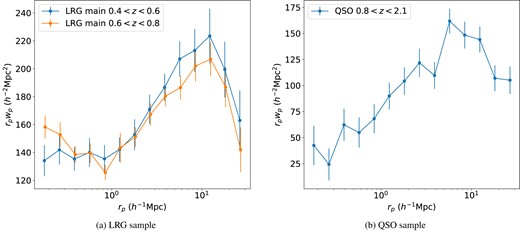
The DESI One-Percent Survey LRG and QSO projected autocorrelation functions multiplied by the projected separation rp. Here, we are only showing LRG clustering in two fiducial redshift bins: 0.4 < z < 0.6 and 0.6 < z < 0.8. For QSOs, we consider one large redshift bin 0.8 < z < 2.1 to achieve a reasonable sample size.
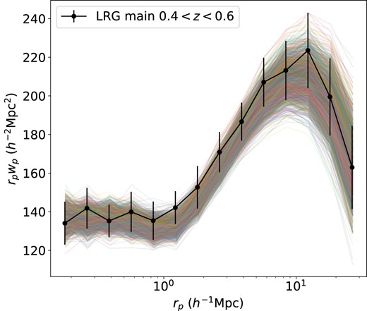
The projected autocorrelation function wp of the 1800 boxes after tuning vanilla HOD parameters to match the clustering of One-Percent Survey LRGs in 0.4 < z < 0.6. See Section 5 for details.
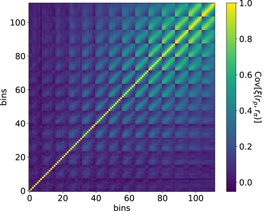
The correlation matrix of One-Percent Survey LRG ξ(rp, rπ) in 0.4 < z < 0.6, generated from the 1800 boxes after tuning to match the observed clustering. The 2D bins of ξ(rp, rπ) are collapsed in this representation as a column-wise stack (the bin number is strictly increasing in rp and periodic in rπ).
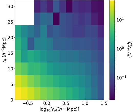
The One-Percent Survey LRG ξ(rp, rπ) in 0.4 < z < 0.6. rp and rπ denote the transverse and LoS separation of the galaxies in comoving units. For this analysis, we only utilize the transverse scales 0.15–32 h−1Mpc. The white section corresponds to negative values, which do not show up on the log scale.
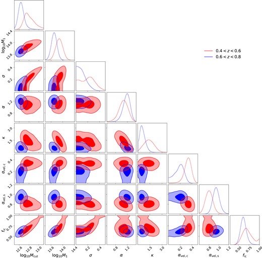
The DESI One-Percent Survey LRG HOD posterior. The red and blue contours correspond to the marginalized posteriors for LRGs in the 0.4 < z < 0.6 and 0.6 < z < 0.8 bins, respectively. We are showing only the 1σ and 2σ contours for clarity. The fact that the blue contours are smaller than the red contours is simply due to the larger sample size in the 0.6 < z < 0.8 bin (sample number density, larger volume). The offset between the contours may suggest mild evolution effects..
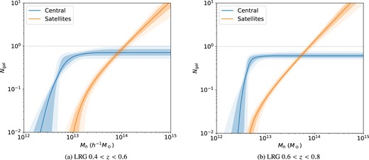
The LRG HOD best fit the posterior. The shaded regions correspond to 1σ and 2σ posteriors (68 and 95 per cent intervals centred around the median prediction). The horizontal dotted line denotes Ngal = 1.
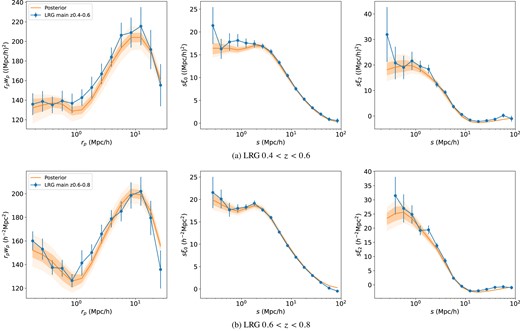
The LRG wp and multipoles posterior predicatives compared to the data. The blue lines correspond to the One-Percent Survey measurement with jack-knife error bars. The solid orange line denotes the posterior mean. The orange shaded regions correspond to the 1σ and 2σ full posterior using the full mock covariance matrix.
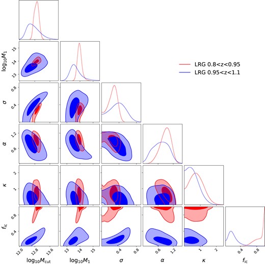
The DESI One-Percent Survey LRG at z > 0.8 HOD posterior. The results from 0.8 < z < 0.95 and 0.95 < z < 1.1 are shown in red and blue, respectively. The contours represent 68 and 95 per cent confidence levels. 1D marginalized distribution for each parameter is shown at the top of each column. Note that the axes do not share the same range as Fig. 6. These contours are also not directly comparable to those in Fig. 6 as we are using a simpler model and a more limited data vector for this high redshift sample. The same note applies to Fig. 10.
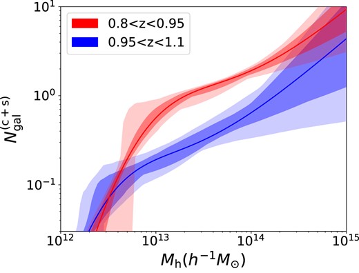
The HOD posterior band (central + satellite) of LRG sample at z > 0.8. The results from 0.8 < z < 0.95 and 0.95 < z < 1.1 are shown in red and blue, respectively. The shaded regions correspond to 1σ and 2σ posteriors.

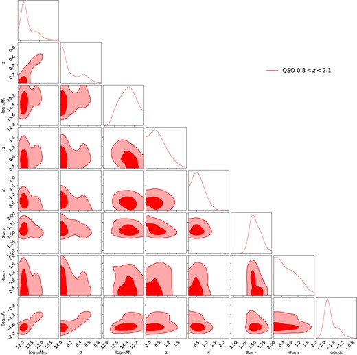
The DESI One-Percent Survey QSO HOD posterior. The red contours correspond to the 1σ and 2σ marginalized posteriors for QSOs in the 0.8 < z < 2.1 bin.
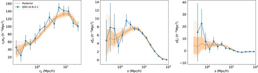
The QSO wp and multipoles posterior predictives compared to the data. The blue lines correspond to the One-Percent Survey measurement with jackknife error bars. The solid orange line denotes the prediction corresponding to the posterior mean. The orange shaded regions correspond to the 1σ and 2σ full posterior using the full mock covariance matrix.
3 SIMULATIONS
To model the underlying dark matter density field, we use the AbacusSummit simulation suite, which is a set of large, high-accuracy cosmological N-body simulations using the AbacusN-body code (Garrison, Eisenstein & Pinto 2019; Garrison et al. 2021; Maksimova et al. 2021). This suite is designed to meet the Cosmological Simulation Requirements of DESI. AbacusSummit consists of over 150 simulations, containing approximately 60 trillion particles at 97 different cosmologies. A base simulation box contains 69123 particles within a (2 h−1Gpc)3 volume, which yields a particle mass of 2.1 × 10⁹ h−1 M⊙.3 All analyses in this paper are done exclusively at the fiducial Planck 2018 cosmology with the AbacusSummit_base_c000_ph000 box.
The simulation output is organized into discrete redshift snapshots. Specifically, we use the z = 0.5 and z = 0.8 snapshots for LRGs at z < 0.8, and the z = 0.8 and z = 1.1 snapshots for LRGs at z > 0.8. For the QSO analysis, due to the very limited sample size, we choose not to divide the sample into multiple redshift bins. Instead, we use the z = 1.4 snapshot for the single redshift bin 0.8 < z < 2.1. A more nuanced analysis of the QSO sample is planned when more data become available.
The dark matter haloes are identified with the CompaSO halo finder, which is a highly efficient on-the-fly group finder specifically designed for the AbacusSummit simulations (Hadzhiyska et al. 2022a). CompaSO builds on the existing spherical overdensity (SO) algorithm by taking into consideration the tidal radius around a smaller halo before competitively assigning halo membership to the particles in an effort to more effectively deblend haloes. Among other features, the CompaSO finder also allows for the formation of new haloes on the outskirts of growing haloes, which alleviates a known issue of configuration-space halo finders of failing to identify haloes close to the centers of larger haloes. We also run a post-processing ‘cleaning’ procedure that leverages the halo merger trees to ‘re-merge’ a subset of haloes. This is done both to remove over-deblended haloes in the spherical overdensity finder, and to intentionally merge physically associated haloes that have merged and then physically separated (Bose et al. 2022).
In addition to periodic boxes, the simulation suite also provides a set of simulation light-cones at the fiducial cosmology (Hadzhiyska et al. 2022b). The basic algorithm associates the haloes from a set of coarsely spaced snapshots with their positions at the time of light-cone crossing by matching halo particles to on-the-fly light-cone particles. The resulting halo catalogues are reliable at Mhalo > 2.1 × 10¹¹ h−1M⊙, more than sufficient for LRGs and QSOs. As part of the data products, we take the best-fitting HODs across different redshift snapshots and construct redshift-dependent LRG mocks on the 25 base light-cones. Each light-cone covering an octant of the sky (∼5156 deg2) up to z ∼ 0.8. We clarify that in this analysis, we only use the cubic boxes to conduct our analysis, the light-cones are only used to produce redshift-dependent mocks as part of the data products.
4 HALO OCCUPATION DISTRIBUTION
To propagate the simulated matter density field to galaxy distributions, we adopt the HOD model, which probabilistically populate dark matter haloes with galaxies according to a set of halo properties. Statistically, the HOD can be summarized as a probabilitistic distribution |$P(n_g|\boldsymbol{X}_h)$|, where ng is the number of galaxies of the given halo, and |$\boldsymbol{X}_h$| is some set of halo properties.
In the vanilla HOD model, halo mass is assumed to be the only relevant halo property |$\boldsymbol{X}_h = {M_h}$| (Zheng et al. 2005; Zheng, Coil & Zehavi 2007). This vanilla HOD separates the galaxies into central and satellite galaxies, and assumes the central galaxy occupation follows a Bernoulli distribution whereas the satellites follow a Poisson distribution, in which case one only needs to specify the mean occupation per halo |$\bar{n}_{\mathrm{cent}}$| and |$\bar{n}_{\mathrm{sat}}$|. Beyond the vanilla model, galaxy occupation can also depend on secondary halo properties beyond halo mass, an phenomenon commonly referred to as galaxy assembly bias or galaxy secondary bias (see Wechsler & Tinker 2018, for a review). While galaxy assembly bias is well physically motivated, many studies have looked for it both in simulations and data (e.g. Wechsler et al. 2002; Croton, Gao & White 2007; Gao & White 2007; Lin et al. 2016; Hadzhiyska et al. 2020; Xu, Zehavi & Contreras 2021a; Xu et al. 2021b; Delgado et al. 2022; Salcedo et al. 2022; Wang et al. 2022; Yuan et al. 2022b) with mixed results.
For this analysis, we use the AbacusHOD code to find best-fitting HODs and sample HOD posteriors. AbacusHOD is a highly efficient HOD implementation that enables a large set of HOD extensions (Yuan et al. 2021b). The code is publicly available as a part of the abacusutils package at https://github.com/abacusorg/abacusutils. Example usage can be found at https://abacusutils.readthedocs.io/en/latest/hod.html.
4.1 Baseline model
For a LRG sample, the HOD is well approximated by a vanilla model given by (originally shown in Zheng, Coil & Zehavi 2007 and referred to as Zheng07 or vanilla later in the text):
where the five vanilla parameters characterizing the model are Mcut, M1, σ, α, κ. Mcut sets the minimum halo mass to host a central galaxy. M1 roughly sets the typical halo mass that hosts one satellite galaxy. σ controls the steepness of the transition from 0 to 1 in the number of central galaxies. α is the power-law index on the number of satellite galaxies. κMcut gives the minimum halo mass to host a satellite galaxy. We have added a modulation term |$\bar{n}_{\mathrm{cent}}^{\mathrm{LRG}}(M)$| to the satellite occupation function to mostly remove satellites from haloes without centrals.4 We have also included an incompleteness parameter fic, which is a downsampling factor controlling the overall number density of the mock galaxies. This parameter is relevant when trying to match the observed mean density of the galaxies in addition to clustering measurements. By definition, 0 < fic ≤ 1.
For QSOs, we adopt essentially the same HOD model except we remove the central modulation term in the satellite occupation as there is no evidence that the existence of satellite QSOs are strongly associated with central QSOs. Thus, for satellite QSOs, we have
In addition to determining the number of galaxies per halo, the standard HOD model also dictates the position and velocity of the galaxies. In the vanilla model, the position and velocity of the central galaxy are set to be the same as those of the halo center, specifically the L2 subhalo centre-of-mass for the CompaSO haloes (see Hadzhiyska et al. 2022a). For the satellite galaxies, they are randomly assigned to halo particles with uniform weights, each satellite inheriting the position and velocity of its host particle.
Because we are modelling the full-shape ξ(rp, rπ), we also include an additional level of flexibility in the velocity model known as velocity bias in the baseline model. Velocity bias essentially parametrizes any biases the velocities of the central and satellite galaxies relative to their, respectively, host haloes and particles. This is shown to to be a necessary ingredient in modelling BOSS LRG redshift-space clustering on small scales (e.g. Guo et al. 2015a; Yuan et al. 2021b). Velocity bias has also been identified in hydrodynamical simulations and measured to be consistent with observational constraints (e.g. Ye et al. 2017; Yuan et al. 2022b).
We parametrize velocity bias through two additional parameters:
- αvel,c is the central velocity bias parameter, which modulates the peculiar velocity of the central galaxy relative to the halo centre along the LoS. Specifically in this model, the central galaxy velocity along the LoS is thus given by(7)$$\begin{eqnarray} v_\mathrm{cent, z} = v_\mathrm{L2, z} + \alpha _\mathrm{vel, c} \delta v(\sigma _{\mathrm{LoS}}), \end{eqnarray}$$
where vL2,z denotes the LoS component of the central subhalo velocity, δv(σLoS) denotes the Gaussian scatter of the host halo particle velocities, and αvel,c is the central velocity bias parameter. By definition, αvel,c = 0 corresponds to no central velocity bias. We also define αvel,c as non-negative, as negative and positive αc are fully degenerate observationally.
- αvel,s is the satellite velocity bias parameter, which modulates how the satellite galaxy peculiar velocity deviates from that of the local dark matter particle. Specifically, the satellite velocity is given by(8)$$\begin{eqnarray} v_\mathrm{sat, z} = v_\mathrm{L2, z} + \alpha _\mathrm{vel, s} (v_\mathrm{p, z}-v_\mathrm{L2, z}), \end{eqnarray}$$
where vp,z denotes the line-of-sight component of particle velocity, and αvel,s is the satellite velocity bias parameter. αvel,s = 1 indicates no satellite velocity bias, i.e. satellites perfectly track the velocity of their underlying particles.
To summarize, the baseline HOD model for both LRGs and QSOs is fully specified with the following 8 parameters: (1) 5 vanilla HOD parameters Mcut, M1, σ, α, κ; (2) an incompleteness parameter fic; (3) velocity bias parameters αvel,c and αvel,s.
4.2 Model extensions
AbacusHOD also enables additional physically motivated HOD extensions. In the following analysis, we will test whether the data favour the inclusion of such extensions. We summarize the relevant extensions for LRGs here and refer the readers to Yuan et al. (2021b) for more details:
Acent or Asat are the concentration-based secondary bias parameters for centrals and satellites, respectively. Also known as galaxy assembly bias parameters. Acent = 0 and Asat = 0 indicate no concentration-based secondary bias in the centrals and satellites occupation, respectively. A positive A indicates a preference for lower concentration haloes, and vice versa.
Bcent or Bsat are the environment-based secondary bias parameters for centrals and satellites, respectively. The environment is defined as the mass density within a renv = 5 h−1Mpc tophat of the halo centre, excluding the halo itself. Bcent = 0 and Bsat = 0 indicate no environment-based secondary bias. A positive B indicates a preference for haloes in less dense environments, and vice versa.
s is the satellite profile bias parameter, which modulates how the radial distribution of satellite galaxies within haloes deviate from the radial profile of the halo (potentially due to baryonic effects). s = 0 indicates no radial bias, i.e. satellites are uniformly assigned to halo particles. s > 0 indicates a more extended (less concentrated) profile of satellites relative to the halo, and vice versa.
For this paper, we will add each of these extensions on to the 8-parameter baseline HOD model and conduct fits on the data. We compare the fits to study whether any of these extensions are favoured. However, we only test these extensions on the LRG sample. While similar extensions might also apply for QSOs, we lack the sufficient sample size to meaningfully constrain such effects.
4.3 Redshift-space distortion
Having generated the mock galaxy catalogues with each HOD prescription, we need to compute the 2PCF to compare to the data. However, because the data is in redshift space, meaning the observed LoS positions of galaxies are shifted by their peculiar velocity divided by the Hubble constant, we need to incorporate this effect in our model too. Thus, we impose RSD on the z-axis positions of the mock galaxies by amount
where Zreal and Zredshift are the real and redshift-space z-axis positions of the galaxies. vpec, Z is the galaxy peculiar velocity projected along the z-axis. H(z) is the Hubble parameter at redshift z. The 1 + z scaling converts the coordinates into comoving units.
Finally, we compute the model predicted ξ(rp, rπ) directly from mocks, assuming z-axis as the LoS direction. We use the grid-based 2PCF calculator Corrfunc (Sinha & Garrison 2020) for efficiency.
5 LIKELIHOOD MODEL AND COVARIANCE MATRIX
To perform the subsequent optimizations and sampling of the HOD parameters, we need to construct a likelihood function. In this analysis, we assume a simple Gaussian likelihood and utilize the χ2 statistic:
where the ξmodel is the model predicted ξ(rp, π) and ξdata is the DESI measurement. |$\boldsymbol{C}$| is the covariance matrix.
We also include in the likelihood model an additional term related to the mean number density of the sample,
σn is the uncertainty of the galaxy number density. The |$\chi ^2_{n_g}$| is a half normal around the observed number density ndata. When the mock number density is less than the data number density (nmock < ndata), we set the completeness to fic = 1 and give a Gaussian-type penalty on the difference between nmock and ndata. When the mock number density is higher than data number density (nmock ≥ ndata), then we set fic = ndata/nmock such that the mock galaxies catalogue is uniformly downsampled to match the data number density. In this case, we impose no penalty. This definition of |$\chi ^2_{n_g}$| allows for incompleteness in the observed galaxy sample while penalizing HOD models that produce insufficient galaxy number density. For the rest of this paper, we assume σn = 0.1ndata.
Finally, the full χ2 is given by
To obtain the covariance matrix, one could divide the observed sample into jackknife regions and compute the clustering in each assuming they are independent realizations. However, given the finite size of the One-Percent Survey footprint and the relatively large number of bins in the ξ(rp, rπ) statistic, the resulting jackknife covariances are noisy and close to singular. Instead, we opt to use the 1800 |$500 $|h−1Mpc boxes with varying phases in the AbacusSummit suite to generate mock-based covariance matrices. Specifically, each small box shares the same particle resolution as the base boxes and is 500 h−1Mpc per side, which is sufficient for the scales we analyse.
First, we generate mocks on the 1800 boxes that produce the same clustering as that measured in data. Specifically, we take a baseline HOD model and fit the observed ξ(rp, rπ) with just the jackknife errors measured on the data, assuming all off-diagonal terms in the covariance matrices are zero. We achieve good fits for both tracers and in all redshift bins. We do not present the values of this fit to avoid confusion with the final ‘full covariance’ fit presented in Table 3, but the parameter values are consistent with the ‘full covariance’ fits. We then take the best-fitting HOD and populate the 1800 covariance boxes, from which compute the covariance matrices. Finally, we renormalize the covariance matrix by keeping the mock-based correlation matrix and using the data-based jackknife diagonal errors to convert the correlation matrix to the final covariance matrix.
Comparing LRG HOD model extensions in both redshift bins. The baseline model refers to the standard vanilla 5-parameter model plus velocity bias and incompleteness. A refers to galaxy assembly bias parametrized in terms of halo concentration. B refers to galaxy assembly bias parametrized in terms of the local environment. s refers to 1-halo satellite profile modulations. The AIC scores suggest that none of the extended models are preferred over the baseline model. More details of the best-fits are given in Table 3.
| LRG | 0.4 < z < 0.6 | 0.6 < z < 0.8 | ||
|---|---|---|---|---|
| Model | χ2/d.o.f. | AIC | χ2/d.o.f. | AIC |
| Baseline | 1.03 | 130 | 0.99 | 125 |
| Baseline + A | 1.05 | 133 | 0.98 | 125 |
| Baseline + B | 1.05 | 133 | 0.99 | 126 |
| Baseline + s | 1.06 | 131 | 1.01 | 126 |
| LRG | 0.4 < z < 0.6 | 0.6 < z < 0.8 | ||
|---|---|---|---|---|
| Model | χ2/d.o.f. | AIC | χ2/d.o.f. | AIC |
| Baseline | 1.03 | 130 | 0.99 | 125 |
| Baseline + A | 1.05 | 133 | 0.98 | 125 |
| Baseline + B | 1.05 | 133 | 0.99 | 126 |
| Baseline + s | 1.06 | 131 | 1.01 | 126 |
Priors used for LRG and QSO HOD fits. We use broad Gaussian priors on all parameters. We also quote the bounds we impose in addition to the Gaussian priors. Units of mass are in h−1 M⊙.
| Params | LRG | QSO | ||
|---|---|---|---|---|
| Prior | Bounds | Prior | Bounds | |
| log Mcut | |$\mathcal {N}(13.0,1.0)$| | [12,13.8] | |$\mathcal {N}(12.7, 1)$| | [11.2, 14.0] |
| log M1 | |$\mathcal {N}(14.0,1.0)$| | [12.5,15.5] | |$\mathcal {N}(15.0, 1)$| | [12.0, 16.0] |
| σ | |$\mathcal {N}(0.5,0.5)$| | [0.0,3.0] | |$\mathcal {N}(0.5, 0.5)$| | [0.0, 3.0] |
| α | |$\mathcal {N}(1.0,0.5)$| | [0.0,2.0] | |$\mathcal {N}(1.0, 0.5)$| | [0.3, 2.0] |
| κ | |$\mathcal {N}(0.5,0.5)$| | [0.0,10.0] | |$\mathcal {N}(0.5, 0.5)$| | [0.3, 3.0] |
| αc | |$\mathcal {N}(0.4,0.4)$| | [0.0, 1.0] | |$\mathcal {N}(1.5,1.0)$| | [0.0, 2.0] |
| αs | |$\mathcal {N}(0.8,0.4)$| | [0.0, 2.0] | |$\mathcal {N}(0.2, 1.0)$| | [0.0, 2.0] |
LRG and QSO marginalized posteriors, with different models and different measurements. The error bars are 1σ uncertainties. We also display several derived parameters, specifically the marginalized satellite fraction fsat, the sample completeness fic, the average halo mass per galaxy |$\log \overline{M}_\mathrm{h}$|, and the linear biasblin. Units of mass are given in h−1 M⊙.
| Tracer | LRG 0.4 < z < 0.6 | LRG 0.6 < z < 0.8 | QSO 0.8 < z < 2.1 | |||
|---|---|---|---|---|---|---|
| Model | Zheng07 + fic | Zheng07 + fic | Zheng07 + fic | Zheng07 + fic | Zheng07 + fic | Zheng07 + fic |
| +αc + αs | +αc + αs | +αc + αs | ||||
| Data | wp + nz | ξ(rp, rπ) +nz | wp + nz | ξ(rp, rπ) +nz | wp + nz | ξ(rp, rπ) +nz |
| log Mcut | 12.89|$^{+0.11}_{-0.09}$| | 12.79|$^{+0.15}_{-0.07}$| | 12.78|$_{-0.08}^{+0.10}$| | 12.64|$^{+0.17}_{-0.05}$| | 12.67|$_{-0.36}^{+0.71}$| | 12.2|$^{+0.6}_{-0.1}$| |
| log M1 | 14.08|$^{+0.10}_{-0.10}$| | 13.88|$^{+0.11}_{-0.11}$| | 13.94|$_{-0.11}^{+0.14}$| | 13.71|$^{+0.07}_{-0.07}$| | 15.00|$_{-0.64}^{+0.62}$| | 14.7|$^{+0.6}_{-0.6}$| |
| σ | 0.19|$^{+0.12}_{-0.12}$| | 0.21|$^{+0.11}_{-0.10}$| | 0.17|$_{-0.11}^{+0.10}$| | 0.09|$^{+0.09}_{-0.05}$| | 0.42|$_{-0.25}^{+0.26}$| | 0.12|$^{+0.28}_{-0.06}$| |
| α | 1.20|$^{+0.15}_{-0.19}$| | 1.07|$^{+0.13}_{-0.16}$| | 1.07|$_{-0.21}^{+0.16}$| | 1.18|$^{+0.08}_{-0.13}$| | 1.09|$_{-0.37}^{+0.43}$| | 0.8|$^{+0.4}_{-0.2}$| |
| κ | 0.65|$^{+0.45}_{-0.39}$| | 1.4|$^{+0.6}_{-0.5}$| | 0.55|$_{-0.34}^{+0.42}$| | 0.6|$^{+0.4}_{-0.2}$| | 0.74|$_{-0.29}^{+0.41}$| | 0.6|$^{+0.8}_{-0.2}$| |
| αc | – | 0.33|$^{+0.05}_{-0.07}$| | – | 0.19|$^{+0.06}_{-0.09}$| | – | 1.54|$^{+0.17}_{-0.08}$| |
| αs | – | 0.80|$^{+0.07}_{-0.07}$| | – | 0.95|$^{+0.07}_{-0.06}$| | – | 0.6|$^{+0.6}_{-0.3}$| |
| fic | 0.92|$^{+0.08}_{-0.17}$| | 0.70|$^{+0.15}_{-0.09}$| | 0.89|$_{-0.14}^{+0.11}$| | 0.62|$^{+0.07}_{-0.06}$| | 0.041|$_{-0.016}^{+0.066}$| | 0.019|$^{+0.029}_{-0.004}$| |
| fsat | 0.089|$_{-0.010}^{+0.013}$| | 0.106|$^{+0.011}_{-0.012}$| | 0.104|$_{-0.010}^{+0.013}$| | 0.136|$^{+0.011}_{-0.010}$| | 0.05|$_{-0.05}^{+0.26}$| | 0.03|$^{+0.08}_{-0.02}$| |
| |$\log \overline{M}_\mathrm{h}$| | 13.42|$_{-0.02}^{+0.02}$| | 13.40|$^{+0.02}_{-0.02}$| | 13.26|$_{-0.02}^{+0.02}$| | 13.24|$_{-0.02}^{+0.02}$| | 12.84|$_{-0.08}^{+0.14}$| | 12.65|$^{+0.09}_{-0.04}$| |
| blin | |$1.94_{-0.04}^{+0.04}$| | |$1.88_{-0.03}^{+0.03}$| | |$2.11_{-0.04}^{+0.03}$| | |$2.06_{-0.02}^{+0.02}$| | |$2.50_{-0.10}^{+0.22}$| | |$2.31_{-0.05}^{+0.06}$| |
| χ2/d.o.f | 4.5/(14-5) | 108/(112-7) | 19.6/(14-5) | 104/(112-7) | 16.0/(14-5) | 101/(112-7) |
Fig. 3 serves as a visualization of the 1800 realizations after tuning to match the observed ξ(rp, rπ), where we overlay the projected autocorrelation functions of the 1800 boxes on the observation. We see that the mock realizations do well in producing the observed clustering, and the spread in the mock clustering is consistent in trend with the data jackknife errorbars.
Fig. 4 shows the resulting correlation matrix computed from the 1800 mocks for the LRG ξ(rp, rπ) in 0.4 < z < 0.6. The 2D bins of ξ(rp, rπ) are collapsed in this representation as a column-wise stack (the bin number is strictly increasing in rp and periodic in rπ). We see that the off-diagonal terms are determined with high signal-to-noise, a result of the large number of realizations and the large volume available with the 1800 boxes. The large-scale bins are correlated as they become sample variance dominated by large-scale structure, whereas the small-scale bins are largely independent, as they are dominated by the shot noise of galaxy occupation.
We similarly generate mock covariance matrices for the LRG sample in 0.6 < z < 0.8 and the QSO sample. We omit those plots for brevity. The covariance matrix for the LRG sample in 0.6 < z < 0.8 share essentially the same structure as the lower redshift LRG sample, with shot noise dominating the smallest scales and sample variance becoming significant at larger scales. For QSOs, all scales are dominated by shot noise and the covariance matrix is essentially diagonal. Throughout the rest of this paper, we use these set of mock covariance matrices for model comparison and posterior sampling.
Having defined the likelihood function, we use optimization routines and posterior samplers to evaluate the best-fits and posterior constraints, respectively. Finally, we note that a correction term to the likelihood is applied to correct for the finite number of independent realizations used to calculate the covariance matrix (Hartlap, Simon & Schneider 2007). Due to a large number of mock realizations (∼1800), the correction factor is small but not negligible (|$\sim 6~{{\ \mathrm{per\,cent}}}$|).
6 LRG HOD RESULTS
In this section, we present the results of the One-Percent Survey LRG HOD analysis by deriving the HOD best fits, testing possible model extensions, and presenting the posterior constraints.
6.1 LRG at z < 0.8
We first examine the LRG main sample at z < 0.8, where the number density remains relatively constant. This is also the LRG sample that will be used for DESI Y1 fiducial cosmology analyses. We analyse this sample in two separate redshift bins: 0.4 < z < 0.6 and 0.6 < z < 0.8, using the z = 0.5 and z = 0.8 snapshots, respectively. We target the ξ(rp, rπ) + n(z) data vector in each bin and incorporate the full covariance matrix built on mocks. Fig. 5 shows the LRG ξ(rp, rπ) data vector in 0.4 < z < 0.6. We omit the visualizations for the other redshift bin for brevity. We only utilize the transverse scales 0.15–32 h−1Mpc and LoS separation from 0 to |$32 $|h−1Mpc.
We first test for potential extensions to the 8-parameter baseline HOD model (5-parameter vanilla HOD plus velocity bias plus incompleteness). Specifically, we run optimizations with extended models that include either galaxy assembly bias or satellite radial profile parameter in addition to the baseline parameters. We use a global optimization routine called Covariance matrix adaptation evolution strategy (CMA-ES) with 400 random walkers. We compute the model Akaike Information Criterion (AIC) scores from the best-fitting χ2 and summarize the results in Table 1. The AIC scores essentially calculates the best-fit χ2 but compensating for the number of parameters. Models with lower AIC scores are preferred by the data, and a ΔAIC = 1 roughly corresponds to 1σ significance.
Our tests show no evidence for either flavours of galaxy assembly bias or a satellite radial profile parameter. We conclude that the current data vectors favour the baseline model, and we will conduct the rest of this analysis with just the baseline HOD model. However, Yuan et al. (2021b) found significant evidence for galaxy assembly bias in a similar HOD analysis of BOSS CMASS LRGs. This discrepancy is explained by the significantly larger sample size in CMASS (∼600 000). The factor 10 decrease in sample size translates to a factor 3 increase in statistical error, which in turn downgrades an assembly bias signal as detected in Yuan et al. (2021b) to less than 1σ significance.
Next, we obtain the parameter posteriors for the baseline model in each redshift bin. To sample the HOD posterior, we use the efficient dynesty nested sampler (Speagle & Barbary 2018; Speagle 2020). Again, we use ξ(rp, rπ) as our primary data vector in each redshift bin and include the full covariance matrix in the likelihood evaluation. We incorporate broad multivariate Gaussian priors as quoted in Table 2. We specifically test our choice of Gaussian priors will not significantly bias our main results (see Appendix B for details). We also impose bounds to limit the range explored by the sampler (also documented in Table 2). The resulting marginalized posteriors are presented in Fig. 6 and summarized in Table 3. We visualize the corresponding HOD posteriors in Fig. 7, where the shaded bands denote the 1σ and 2σ constraints (68 and 95 per cent intervals).
Fig. 6 shows several interesting degeneracies. Perhaps the most prominent degeneracy is between parameter log Mcut and σ. Both parameters control the occupation distribution of the centrals, which for LRGs translates to controlling the clustering amplitude of the 2-halo term on large scales. log Mcut controls the mass scale whereas σ controls the slope of the Ncent turn-on. Thus, it makes sense that the two are somewhat degenerate as either a slower turn on (larger σ) or a lower mass scale would decrease the mean bias of the sample.
Similarly, we see a degeneracy between the completeness parameter fic and the central occupation parameters log Mcut and σ. This is due to the constraints on the average density of the galaxy sample. Lower typical halo masses for the galaxies would mean a lower completeness. There is also an interesting degeneracy between log Mcut and log M1, which has been previously discussed in Avila et al. (2020). This is interesting because log M1 controls the halo mass of the satellite galaxies. Thus, a degeneracy between these two parameters suggests a strong constraint on the satellite fraction, and by extension a strong constraint on the relative amplitude of the 1-halo clustering and 2-halo clustering.
The inferred satellite fraction is |$11\pm 1~{{\ \mathrm{per\,cent}}}$| for LRGs in 0.4 < z < 0.6 and |$14\pm 1~{{\ \mathrm{per\,cent}}}$| in 0.6 < z < 0.8, consistent with 11 per cent inferred for the CMASS sample in 0.45 < z < 0.6 (Yuan et al. 2021b) and |$13\pm 3~{{\ \mathrm{per\,cent}}}$| inferred with eBOSS LRGs between 0.6 < z < 0.9 (Zhai et al. 2017).5 The mean halo mass of the LRGs is strongly constrained. We find |$\log _{10}\overline{M}_h=13.40^{+0.02}_{-0.02}$| for 0.4 < z < 0.6 and |$\log _{10}\overline{M}_h=13.24^{+0.02}_{-0.02}$| for 0.6 < z < 0.8. In comparison, Yuan et al. (2021a) found |$\log _{10}\overline{M}_h = 13.60$| for the CMASS sample, and Zhai et al. (2017) found |$\log _{10}\overline{M}_h = 13.4$| for the higher redshift eBOSS sample. Both values are higher than the average halo mass inferred for DESI One-Percent Survey LRGs. This is expected as the DESI sample is fainter and higher number density, thus occupying less massive haloes. Our results also compare well with earlier results from CMASS DR10, which reported a 9–10 per cent satellite fraction for a red luminosity-limited sample with half the DESI density (Guo et al. 2014). The difference in average halo mass between the two redshift bins can simply be attributed to halo growth at fixed density.
The linear bias factor is also calculated in our study by comparing the real-space clustering amplitudes of galaxies with predictions made by the linear theory, specifically
where ξgal denotes the real-space two-point correlation functions of galaxies, and ξlin denotes the theoretical linear matter correlation function at the mean redshift in the respective redshift bin. We compute correlation function using 40 linear bins from 40 to 80 h−1Mpc. ξlin is measured with CLASS (Lesgourgues 2011). For each sample of the MCMC chain, ξgal is measured through the generation of a real-space mock, based on the corresponding HOD parameters. blin is then calculated by performing a constant fitting across all 40 bins, under the assumption of uniform weighting. This process renders blin a derived parameter of the full posterior, which we summarize with mean and standard deviation. The LRG linear bias is 1.88 ± 0.03 in the redshift range of 0.4 < z < 0.6 and 2.06 ± 0.02 for LRGs in 0.6 < z < 0.8. We present a more detailed description of redshift evolution in Section 6.3.
The velocity bias constraints are also mostly consistent with BOSS and eBOSS studies. For the 0.4 < z < 0.6 bin, we find significant central velocity bias at |$33^{+5}_{-7}\mathrm{per\,cent}$|, indicating that the peculiar velocity of the central galaxies relative to the central subhaloes are approximately 30 per cent of the halo velocity dispersion. This is qualitatively consistent with previous studies that also found significant central velocity bias, but somewhat larger in amplitude than the CMASS constraints at |$22\pm 2~{{\ \mathrm{per\,cent}}}$| (Guo et al. 2015a; Yuan et al. 2022b). We also find negative satellite velocity bias |$80\pm 7~{{\ \mathrm{per\,cent}}}$|, indicating that the velocity dispersion of satellite galaxies within haloes are 20 per cent less than that of the halo particles at the same radii. This is consistent with Guo et al. (2015a), who found 86 per cent in CMASS, whereas Yuan et al. (2022b) found less significant velocity bias at 98 per cent. In the higher redshift bin 0.6 < z < 0.8, we find a central velocity bias of |$19^{+6}_{-9}\mathrm{per\,cent}$| and a satellite velocity bias |$95^{+7}_{-6}\mathrm{per\,cent}$|. We do not have eBOSS constraints to compare against, but we can check with simulated DESI samples presented in Yuan et al. (2022b), where we applied DESI photometric selection to IllustrisTNG galaxies (Nelson et al. 2018; Pillepich et al. 2018; Springel et al. 2018). There, we found that the mock DESI LRG sample at z = 0.8 has a velocity bias of αc = 0.14 and αs = 0.92, consistent with our constraints here.
We also run the equivalent analyses on the projected 2PCF wp, where we follow the same procedure as for ξ(rp, rπ), but we exclude the two velocity bias parameters from the HOD model. We also employ a tabulation scheme to accelerate the HOD forward model calculation for these wp fits (details in Appendix A). We include the wp marginalized constraints in Table 3. However, for brevity, we skip their visualization. Comparing the marginalized posteriors in Table 3, the wp results are consistent with the ξ(rp, rπ) results. In terms of inferred quantities, the two data vectors also yield mostly consistent results. The only minor discrepancy between the two fits is that the wp fits favour larger Mcut and M1 parameters, and as a result a larger fic. However, this is compensated by differences in the σ constraints, resulting in essentially identical mean halo mass constraints. In other words, both data vectors place strong constraints on the mean halo mass of the galaxies, but neither breaks the Mcut versus σ degeneracy and favour slightly different loci along this degeneracy.
Comparing the posterior means in the two redshift bins, we see several interesting trends. The average halo mass of the LRG sample increases over time. It is expected given that haloes accrete mass over time, and a fixed density sample at lower redshift would occupy the more massive haloes. The satellite fraction also decreases over time. This trend is not as significant but might be interpreted as a result of galaxy mergers. We discuss redshift evolution in more detail in Section 6.3.
Finally, Fig. 8 showcases the predicted distribution of the 2PCF from the ξ(rp, rπ) posteriors. For this visualization, we choose the wp + ξ0 + ξ2 projections of the redshift-space 2PCF because it is difficult to visualize comparisons of the 2D ξ(rp, rπ) function. wp is the projected 2PCF, whereas ξ0, 2 are the monopole and quadruple moments of the redshift-space 2PCF. The blue curves represent the One-Percent Survey measurements, with jackknife errorbars. The orange shaded regions denote the 1σ and 2σ posterior constraints. The solid orange line showcases the posterior mean. Again, we see that the best-fitting models are consistent with the observed clustering well in both redshift bins. However, in the wp comparisons, the model predicts a larger amplitude than the data at the 1-halo and 2-halo transition regime (rp ∼ 1 h−1Mpc) in both redshift bins. This is not a significant discrepancy with the current sample size but potentially points to limitations of halo boundary definitions and possibly environment-dependent galaxy occupation.
6.2 LRG at z > 0.8
As shown in Fig. 1, the number density of the LRG main sample experiences a significant decline beyond a redshift of 0.8, indicating a marked change in the properties of this population due to the imposed colour selection. To further investigate the HOD and shed light on the evolution of the LRG sample in this redshift range, we subdivide the high-redshift LRGs into two redshift intervals, 0.8 < z < 0.95 and 0.95 < z < 1.1. We use the z = 0.8 and z = 1.1 snapshots and employ the Zheng07 + fic model to fit wp + nz data vector using the tabulation method for this aspect of the analysis.
Fig. 9 shows the 1σ and 2σ confidence level contours for the HOD parameters. Due to the higher number density, the fit from the lower redshift interval displays a much tighter constraint as compared to the higher redshift interval, as anticipated. We find similar degeneracies between log Mcut and σ, log Mcut and log M1 as LRGs at z < 0.8. The 1D distribution depicts a change in the mean value of each parameter in the Zheng07 model as the redshift increases. This trend is consistent with the comparison of the 0.4 < z < 0.6 and 0.6 < z < 0.8 bins in Fig. 6. The most notable difference is observed in the incompleteness parameter fic. As fic can effectively control the number density of the mock galaxies, it decreases significantly as the number density of the sample decreases, indicating a drastic increase in incompleteness.
The results of our analysis provide a compelling reason for conducting a detailed study of the HOD of high-redshift LRGs. As shown in Fig. 10, the 1σ and 2σ uncertainty bands of the HOD function for the high-redshift LRG sample have a minimal overlap for the range 12.8 < log Mhalo < 14.2, indicating a significant difference in the HOD between the two redshift intervals. Furthermore, Table 4 summarizes the marginalized statistics for the high-redshift LRG main sample, which show differences in the mean completeness fic (from 92 to 19 per cent), the satellite fraction fsat (from 11.0 to 15.1 per cent), mean halo mass |$\log _{10}\overline{M}_\mathrm{h}$| (from 13.29 to 13.00) and linear bias blin (from 2.31 to 2.13). These results indicate that the HOD of the high-redshift LRG main sample evolves with redshift, and that DESI LRGs at z > 0.95 might have be a physically different sample than the lower redshift LRG sample. We describe several possible explanations in the following subsection.
The results for the fits to high-z LRG sample with two redshift bin: 0.8 < z < 0.95 and 0.95 < z < 1.1. We show the mean±1σ error for HOD and derived parameters. We also list the average comoving number density in units of 10−4 (h−1Mpc)−3. Masses are in units of h−1 M⊙.
| Params | LRG 0.8 < z < 1.1 | |
|---|---|---|
| 0.8 < z < 0.95 | 0.95 < z < 1.1 | |
| log Mcut | 12.89|$_{-0.13}^{+0.12}$| | 12.68|$_{-0.26}^{+0.38}$| |
| log M1 | 13.96|$_{-0.14}^{+0.15}$| | 13.60|$_{-0.29}^{+0.47}$| |
| σ | 0.26|$_{-0.13}^{+0.09}$| | 0.37|$_{-0.20}^{+0.18}$| |
| α | 0.91|$_{-0.22}^{+0.18}$| | 0.72|$_{-0.34}^{+0.31}$| |
| κ | 0.74|$_{-0.42}^{+0.46}$| | 0.51|$_{-0.33}^{+0.43}$| |
| fic | 0.92|$_{-0.18}^{+0.08}$| | 0.19|$_{-0.07}^{+0.14}$| |
| fsat | 0.110|$_{-0.012}^{+0.016}$| | 0.151|$_{-0.041}^{+0.048}$| |
| |$\log _{10}\overline{M}_\mathrm{h}$| | 13.29|$_{-0.02}^{+0.02}$| | 13.00|$_{-0.03}^{+0.03}$| |
| blin | |$2.31_{-0.04}^{+0.04}$| | |$2.13_{-0.05}^{+0.05}$| |
| |$\overline{n_z}$| | 4.56 | 1.84 |
6.3 Redshift evolution of DESI LRG HOD
The evolution of HOD and derived parameters of LRGs across all redshift bins are shown in Fig. 11. We only use data vector wp + n(z) in this part of the analysis for consistency. The central galaxy host halo mass threshold (Mcut) does not exhibit any significant trend with redshift within the uncertainties. The scatter in the halo mass threshold (σ) tends to increase with increasing redshift, indicating a smoother transition in the central HOD on high redshift. In terms of satellite parameters, both M1 and α show a declining trend with redshift, while κ shows little variation with redshift and is weakly constrained by the data.
The satellite fraction (fsat) shows a mild trend of increasing with redshift at z < 0.95, rising from |$f_\mathrm{sat}\simeq 9~{{\ \mathrm{per\,cent}}}$| at z ≃ 0.5 to |$f_\mathrm{sat}\simeq 11~{{\ \mathrm{per\,cent}}}$| at z ≃ 0.9. This increase in satellite fraction can be interpreted as a result of the merging of galaxies over time. At z > 0.95, the satellite fraction increases substantially to 15 per cent, but the significance is low.
The mean halo mass does not exhibit a clear trend except at z > 0.95, where the mean halo mass drops off substantially. A similar behaviour is seen for the galaxy bias, which increases with redshift at z < 0.95 (consistent with studies of DESI-like photometric LRGs in Zhou et al. 2020) but drops off at z > 0.95. Furthermore, the highest redshift bin also exhibits a drastic drop in completeness. These comparisons serve as strong evidence that that the LRG sample at z > 0.95 is physically different from the LRGs at z < 0.95.
Zhou et al. (2023) showed that the DESI LRG selection should yield a highly stellar mass complete sample at log10M* > 11.5 between redshift 0.4 < z < 0.9. At z > 0.9 the completeness at the high mass end starts to deviate from 1 and drops further at z > 1. This point is confirmed by explicitly computing the stellar mass functions of DESI SV3 LRGs via SED fitting in Gao et al. (2023), where a substantial incompleteness at log10M* > 11.5 is observed at z > 1. This incompleteness at the high-mass end can partially explain the drop in the inferred bias and halo mass in the highest redshift bin.
Another potential contributing effect is that the DESI LRG selection employs a sliding colour–magnitude cut in r − W1 versus W1 that turns over at W1 = ∼ − 19 to include more galaxies at the high redshift end (see fig. 3 of Zhou et al. (2023)). However, this turn over also includes red galaxies with very faint W1 magnitudes into the LRG sample, thus possibly decreasing the mean halo mass and mean galaxy bias.
Separately, Setton et al. (2023) inferred star formation histories from DESI SV1 LRG SEDs and found evidence that recently quenched (post-starburst) galaxies constitute a growing fraction of the massive galaxy population with increasing redshift. The study showed that these galaxies are significantly brighter than the parent LRG sample at fixed stellar mass. Thus, at fixed brightness, these galaxies likely have lower halo masses and lower biases compared to the parent LRG sample. If these galaxies are indeed a significant fraction of high redshift LRGs, then they would contribute to the drop in the mean halo mass and bias. This could also explain the relative high satellite fraction as recently accreted satellites are also likely to have been recently quenched.
An important caveat to consider in the interpretation of the mean halo masses relates to the use of fixed redshift snapshots in this analysis. To obtain an unbiased HOD parameter estimation, the mean redshift of the redshift bin must remain close to the snapshot redshift. However, the choice of snapshots is limited to several primary redshifts provided by the AbacusSummit simulation. For instance, we use the snapshot at z = 0.8 for both 0.6 < z < 0.8 and 0.8 < z < 0.95 redshift bins, resulting in mean sample redshifts that are lower and higher than the snapshot redshift, respectively. As a result, the mean halo mass has been overestimated for 0.8 < z < 0.95 and underestimated for 0.6 < z < 0.8. This effect is particularly pronounced for the 0.95 < z < 1.1 redshift bin, as the drop in number density results in a more significant bias of the mean sample redshift from the snapshot redshift of z = 1.1. Mitigating this effect could, to some extent, resolve the non-monotonic shape in the mean halo mass evolution. Nevertheless, we maintain that this effect does not fully explains the drop in halo mass in the highest redshift bin because the drop in linear bias is agnostic to simulation snapshots as the underlying clustering amplitude is computed at the mean redshift of the sample instead of the simulation snapshot.
This systematic highlights the need for future redshift evolution studies to use more accurate redshifts. The shift in the mean value of HOD and derived parameters also provide a strong scientific incentive to conduct a detailed study of LRGs using the halo light-cone catalogues in combination with a redshift-evolved HOD model.
7 QSO HOD RESULTS
We analyse the QSO sample following the same procedure. First, we construct the mock-based covariance matrix by fitting a baseline HOD on the QSO ξ(rp, rπ) measurement. However, we find that directly fitting ξ(rp, rπ) returns poor fits because the QSO ξ(rp, rπ) measurement below |$r_p \sim 1 $|h−1 Mpc have particularly low signal-to-noise, and the corresponding jackknife errors do not behave properly. Instead, we fit just the projected wp with the 5-parameter + incompleteness model, where we do achieve a good fit. Then we independently tune the two velocity bias parameters to match the ξ(rp, rπ) signal at |$r_p \gt 1 $| h−1 Mpc. We again obtain a good fit. With that, we populate the 1800 small boxes and generate a mock-based covariance matrix for QSO ξ(rp, rπ).
Again, we sample the baseline HOD parameter to obtain marginalized posteriors for the QSO HOD. The results are visualized in Fig. 12 and summarized towards the bottom of Table 3. Fig. 14 shows the corresponding HOD posterior. In general, the QSO HOD parameters are much less constrained than the LRG parameters due to the limited sample size. For the same reason, we also do not test additional model extensions as we already achieve an excellent best-fitting χ2 with the baseline model. We will conduct such tests when a significantly larger sample of QSOs become available. We also showcase the wp-only constraints in Table 3, and we find them to be consistent with the ξ(rp, rπ) constraints.
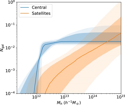
The HOD posterior for the QSO sample. The shaded regions correspond to 1σ and 2σ posteriors.
The HOD constraints compare well with those inferred for eBOSS QSOs as presented in table 1 of Alam et al. (2020). Specifically, they found log Mcut = 12.2 and log M1 = 14.1, consistent with our findings. Perhaps the most unexpected parameter constraint is the central velocity bias, where we find |$\alpha _c = 1.54^{+0.17}_{-0.08}$|, meaning that the central galaxies exhibit large peculiar velocities relative to the halo centre. There are several potential explanations for this. While one possibility is that it points towards energetic processes within the AGN. We speculate that this may also be due to the rather large redshift uncertainties with the QSO sample (Yu et al. 2024). These redshift errors are made worse by the fact that QSO primary spectral lines such as Mg ii line to C iv suffer from large systematic velocity shifts caused by astrophysical effects (e.g. Richards et al. 2002, 2011; Zarrouk et al. 2018). Another potential explanation is that QSOs preferentially occupy recently merged haloes, resulting in large velocity dispersion relative to the halo centre-of-mass. In the following paragraph, we also show that uncertainties in satellite fraction can also be degenerate with velocity bias. Thus, the large velocity bias in the QSO sample could be due to redshift uncertainties, AGN physics and mergers, and/or uncertainties in satellite fraction.
In terms of derived quantities, we infer a mean halo mass of |$\log _{10}\overline{M}_h= 12.65^{+0.09}_{-0.04}$| for the DESI QSO sample, consistent with the |$\log _{10}\overline{M}_h= 12.7$| found for the eBOSS QSO sample in both Rodríguez-Torres et al. (2017) and Alam et al. (2020). We report a linear bias of |$b_\mathrm{lin}=2.31^{+0.06}_{-0.05}$| at z ≃ 1.5 for the DESI QSO sample, which is slightly lower than the first-year eBOSS quasar sample with blin = 2.45 ± 0.05 at z = 1.55, as found by Laurent et al. (2017). However, considering the error bar, the results are consistent. We infer a satellite fraction of |$3^{+8}_{-2}\mathrm{per\,cent}$| for the QSO sample, consistent with |$f_\mathrm{sat} = 5~{{\ \mathrm{per\,cent}}}$| found in Rodríguez-Torres et al. (2017) using a subhalo abundance matching model but significantly lower than the 30 per cent inferred with a multitracer HOD fit in Alam et al. (2020). The large satellite fraction inferred in Alam et al. (2020) is directly a result of a small inferred α = 0.4, which results in a large number of satellites in low mass haloes. However, we speculate that this result might in fact be degenerate with our finding as most of these satellites in low mass haloes do not have companion centrals due to the low completeness. These ‘rogue’ satellites are ill defined in the vanilla HOD context, and can simply be re-classified as centrals. This could also be connected to the large central velocity bias we found, which could disappear if we re-classify some centrals as satellites, which would naturally have larger velocity dispersion. Our results compare well with earlier SDSS Quasar HOD fits. Shen et al. (2013) obtained a satellite fraction of 7–10 per cent and found the inferred satellite fraction to be dependent on the assumed HOD model. Richardson et al. (2012) obtained a lower satellite fraction of |$\sim 0.1~{{\ \mathrm{per\,cent}}}$| for z ∼ 1.4 quasars.
These types of questions also show that the QSO–halo connection physics is poorly understood. In fact, we use the standard 5-parameter model in this analysis simply because we have no evidence that a different model is favoured. We reserve a more comprehensive analysis of QSO HOD for a future paper when a much larger sample of QSOs becomes available.
8 MOCK PRODUCTS
We apply the best-fitting HODs obtained for the LRG and QSO samples to all 25 base boxes available in AbacusSummit at Planck cosmology to create high fidelity mocks. For each tracer at each redshift snapshot, the total sample volume is 200 h−3 Gpc3 comoving. The volume provided by AbacusSummit is an order of magnitude larger than other simulations of comparable resolution, reaching 5–10 times the volume expected to be observed by DESI. Given the volume and resolution, these mocks are critical for testing and calibrating DESI cosmology pipelines at the necessary precision.
In addition to using just the best-fitting HODs, we also create additional mocks where we perturb the HOD parameters around the best fit to generate mocks that share the same cosmology but differ in bias prescriptions. The perturbations are sampled from the 3σ region of the parameter space around the best-fitting values. We repeat this procedure for both the baseline HOD model and an extended HOD model that also includes environment-based assembly bias B and satellite radial profile parameter s, resulting in a set of mocks that encompass a diverse range of possible HODs.
These variety mocks enable key robustness tests of large-scale cosmology inference pipelines against galaxy–halo connection systematics. Specifically, large-scale cosmology pipelines that utilize the BAO/RSD features or full-shape information often assume a much simpler bias model. As a result, complexities in galaxy–halo connection modeling could become degenerate with cosmology and thus result in systematic bias in the inferred cosmology. Thus, it is essential to test cosmology inference pipelines against a range of mocks with varying bias models and demonstrate that the cosmology inference remains unbiased. We defer a detailed discussion of these tests to a dedicated paper (DESI Collaboration, in preparation).
In addition to constructing cubic mocks, we utilize our best fits to construct redshift-dependent mocks on the AbacusSummit light-cones (Hadzhiyska et al. 2022b). The benefit of having mocks on the light-cone is that they provide an accurate synthetic map of the sky, which is crucial for testing out systematic and observational effects such as fiber collisions. Light-cones also enable explicit modeling of redshift evolution, such as in the forward-modelling pipelines being developed for novel summary statistics (e.g. Hahn et al. 2022; Yuan, Hadzhiyska & Abel 2023). Our procedure for generating light-cone mocks is as follows:
Adopting the AbacusHOD algorithm, we first subsample the halo light-cone catalogues assuming the same envelope as the cubic boxes and pre-compute various assembly bias parameters and decorations to the HOD model.
We read in the best-fitting parameters as we found in Section 6. We linearly interpolate the HOD parameters as a function of redshift, pivoting on the two best-fits in the two redshift bins.
Finally, we generate the galaxy mocks for all tracers/the LRGs at all available redshifts of the 25 fiducial cosmologies, i.e. AbacusSummit_c000_ph000-024. We note that due to the geometry, each of our mocks provides an octant of the sky until z ≈ 0.8, decreasing gradually as we go to higher redshifts.
All said mocks will be made publicly available at a future date as a part of DESI EDR.
9 CONCLUSIONS
In this paper, we present a comprehensive analysis of the HOD of the DESI One-Percent Survey LRG and QSO samples using the AbacusSummit cubic boxes.
For LRGs, we study the sample in two fiducial redshift bins 0.4 < z < 0.6, 0.6 < z < 0.8, which are the bins used for DESI Y1 cosmology analyses. We also present analyses of LRGs at higher redshift in 0.8 < z < 1.1, which constitutes a significant fraction of the DESI LRG sample, but is not yet utilized for cosmology due to significant evolution due to selection. In the two fiducial bins, we compare the baseline HOD model with extended models with galaxy assembly bias and satellite profile bias. We find no evidence for model extensions at current precisions and the baseline model is favoured by the data. For both redshift bins, we constrain the baseline parameter posteriors with the ξ(rp, rπ) data vector and mock-based covariance matrix. The resulting model posteriors produce the correct redshift–space clustering. We find strong constraints on inferred properties such as the average halo mass and the satellite fraction, which are broadly consistent with results from eBOSS and BOSS. We also find consistency between ξ(rp, rπ) fit and wp-only fit. The marginalized posterior constraints are summarized in Table 3. To highlight a few key constraints: the LRG sample in 0.4 < z < 0.6 yields a satellite fraction of |$11\pm 1~{{\ \mathrm{per\,cent}}}$| and a mean halo mass of |$\log _{10}\overline{M}_h=13.40^{+0.02}_{-0.02}$|, whereas the 0.6 < z < 0.8 sample results in a satellite fraction of |$14\pm 1~{{\ \mathrm{per\,cent}}}$| and a mean halo mass of |$\log _{10}\overline{M}_h=13.24^{+0.02}_{-0.02}$| in 0.6 < z < 0.8.
Combining the fiducial analysis at z < 0.8 and high redshift analysis at z > 0.8, we find clear trends of evolution, especially in physical parameters like satellite fraction and mean halo mass. Specifically, the mean halo mass decreases with redshift whereas the satellite fraction increases with redshift. This motivates future redshift evolution studies that should shed light on the physics of the evolution of massive galaxies. The marginalized posterior constraints are summarized in Table 4. We also find the properties of the LRG sample at z > 0.95 to deviate significantly from lower redshift LRG sample. Specifically, the LRGs at z > 0.95 display significantly lower mean halo mass, a very low completeness, a lower mean bias while showing a somewhat high satellite fraction. We offer a few plausible explanations of these differences.
The QSO sample is limited by sample size, and we are not able to conduct meaningful comparisons between different HOD models. Regardless, we derive good fits on the data and present posterior constraints. The marginalized posterior constraints are summarized in Table 3. We infer a satellite fraction of |$3^{+8}_{-2}\mathrm{per\,cent}$| and a mean halo mass of |$\log _{10}\overline{M}_h= 12.65^{+0.09}_{-0.04}$| in redshift range 0.8 < z < 2.1. The inferred mean halo mass is consistent with previous results, but there is some discrepancy in the satellite fraction. We speculate that such discrepancy is model dependent and we intend to revisit of this issue when a significantly larger sample of QSOs become available.
Finally, we leverage our HOD fits to generate a large suite of DESI-like mocks. We highlight mocks with varied HODs that test the robustness of large-scale cosmology pipelines, and light-cone-based mocks that are important for building realism and testing observational systematics.
ACKNOWLEDGEMENTS
This material is based upon work supported by the U.S. Department of Energy (DOE), Office of Science, Office of High-Energy Physics, under Contract No. DE-AC02-05CH11231, and by the National Energy Research Scientific Computing Center, a DOE Office of Science User Facility under the same contract. Additional support for DESI was provided by the U.S. National Science Foundation (NSF), Division of Astronomical Sciences under Contract No. AST-0950945 to the NSF’s National Optical-Infrared Astronomy Research Laboratory; the Science and Technology Facilities Council of the United Kingdom; the Gordon and Betty Moore Foundation; the Heising–Simons Foundation; the French Alternative Energies and Atomic Energy Commission (CEA); the National Council of Science and Technology of Mexico (CONACYT); the Ministry of Science and Innovation of Spain (MICINN), and by the DESI Member Institutions: https://www.desi.lbl.gov/collaborating-institutions. Any opinions, findings, and conclusions or recommendations expressed in this material are those of the author(s) and do not necessarily reflect the views of the U. S. National Science Foundation, the U. S. Department of Energy, or any of the listed funding agencies.
The authors are honored to be permitted to conduct scientific research on Iolkam Du’ag (Kitt Peak), a mountain with particular significance to the Tohono O’odham Nation.
DATA AVAILABILITY
The simulation data are available at https://abacussummit.readthedocs.io/en/latest/. The AbacusHOD code package is publicly available as a part of the abacusutils package at https://github.com/abacusorg/abacusutils. Example usage can be found at https://abacusutils.readthedocs.io/en/latest/hod.html. All mock products will be made available at https://data.desi.lbl.gov.
The MCMC chains generated, along with the clustering measurements used in this study – encompassing correlation functions and covariance matrices – are available in a machine-readable format at https://doi.org/10.5281/zenodo.7972386.
Footnotes
For more details, see https://abacussummit.readthedocs.io/en/latest/abacussummit.html
There is evidence that such central-less satellites may exist in a realistic stellar-mass selected catalogue (Jiménez et al. 2019). We include this term for consistency with previous works, but it should have minimal impact on clustering.
We clarify that the reported satellite fraction refers to the fraction of LRGs that are satellites. We are not making statements about intrinsic halo richness.
References
APPENDIX A: ACCELERATING HOD FITTING WITH TABULATION METHOD
In the standard procedure for fitting the HOD model, galaxy mock populations are generated for each set of HOD parameters that have been sampled. The clustering statistic of interest is subsequently measured and compared to measurements obtained from the data in order to estimate the likelihood. This procedure is repeated multiple times for various HOD parameters until the posterior likelihood has been thoroughly explored. An alternative approach, known as the tabulation method, was first proposed by Neistein et al. (2011) and later expanded upon by Zheng & Guo (2016). This method reverses the order of applying the HOD model and measuring the clustering. Specifically, the clustering of haloes is pre-computed prior to the Markov Chain Monte Carlo (MCMC) stage, and the HOD population scheme is subsequently applied by combining weights with the halo clustering. This approach significantly improves the efficiency of the HOD fitting process, as the most computationally intensive step is moved outside of the MCMC loop. We summarize the tabulation method for the AbacusSummit simulation below but refer the reader to Zhang et al. (2022) for more details.
We take projected 2PCF wp here as an example and assume our HOD model only depend on the mass of the host halo. To match the behaviour of AbacusHOD, where we populate the satellite with particles, we first divide the halo catalogue and particle catalogue attached to the haloes into Nb bins. Then the galaxy correlation function wp,gg is given by a weighted sum over different mass bin cross-correlations.
where wp,hh(rp, Mi, Mj) is the two-point cross-correlation function of haloes in the ith and jth mass bins (similarly for the halo–article and particle–particle correlation functions) and naively we could take the weight as
where |$N_\mathrm{h}^i$| and |$N_\mathrm{p}^i$| are numbers of haloes and particles in ith mass bin. Equation (A1) gives an average value of clustering expected for a given HOD model instead of a specific realisation that includes stochastic noise and further reduces the bias of HOD fitting. We also test and confirm that the mean prediction is consistent with the output of the standard AbacusHOD approach.
While the tabulation method can accelerate the fitting of HOD, it also limits the flexibility of extending the HOD model. The baseline HOD model relies solely on halo mass, making it easy to prepare tabulated halo and particle pair counts across mass bins. However, when dealing with more complex HOD models that involve velocity bias and assembly bias extensions, additional dimensions of dependency can significantly increase the complexity of preparing tabulated halo and particle pair counts. Therefore, we only employ the tabulation method to quickly evaluate the HOD posterior when using the Zheng07 + fic model to fit the wp + nz data vector. For all other cases, we use the standard AbacusHOD approach.
APPENDIX B: CHOICE OF PRIOR
The selection of priors for the HOD parameters can potentially impact the inferred constraints. In order to eliminate extreme values of the HOD parameters and gain a more comprehensive understanding of the Galaxy–Halo connection model, Gaussian priors shown in Table 2 were applied to the HOD parameters in the primary analysis. In order to assess the potential impact of these priors on the results, additional MCMC analyses were conducted using only flat priors.
In this test, we employ the Zheng07 + fic model to fit wp + nz of LRG at redshift 0.6 < z < 0.8. Fig. B1 illustrates the 1σ and 2σ confidence level contours for the HOD parameters when different priors are applied. It is clear that the fit with a Gaussian prior displays a tighter contour, particularly for the satellite parameters log10M1, α, and κ. The Gaussian prior helps to eliminate isolated regions in the contour, where the data have limited power to constrain the parameters. The 1D distribution of each parameter in Fig. B1 indicates that the Gaussian prior has a smaller impact on the central parameters as compared to the satellite parameters and hardly any impact on incompleteness.
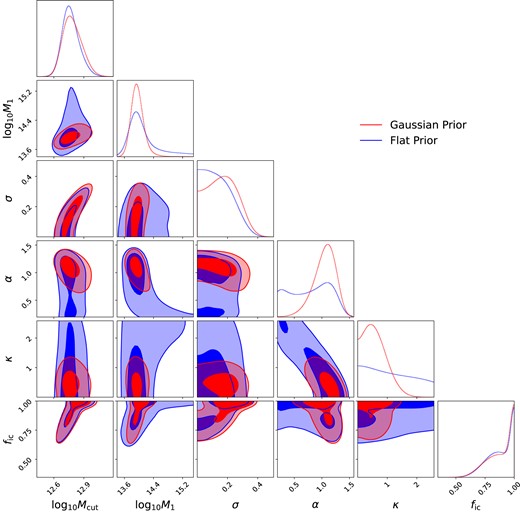
Marginalized probability distribution of HOD parameters for LRG sample at 0.6 < z < 0.8 with and without Gaussian priors listed in Table 2. The results using Gaussian prior and flat prior are shown in red and blue, respectively. The contours represent 68 and 95 per cent confidence levels. 1D marginalized distribution for each parameter is shown at the top of each column.
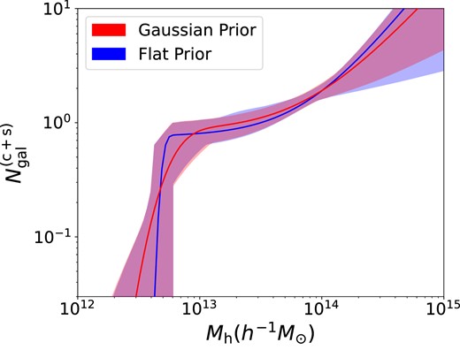
2σ band of LRG sample HOD at 0.6 < z < 0.8 with and without Gaussian prior. The red is the 95 per cent CL uncertainty from fit using Gaussian priors, the blue is the 95 per cent CL uncertainty from fit using flat priors. Lines are the corresponding best fit.
Fig. B2 shows the 2σ uncertainty band of HOD posterior and best fit for both cases. The two bands overlap heavily with each other. The Gaussian prior fit has a slightly narrower band for log10Mcut > 14.2, where the satellite parameters have a larger impact on the HOD. Additionally, the Gaussian prior presents a smoother best fit than the flat prior, which exhibits a distinct step on the lower mass end. As a result, our choice of Gaussian prior help removes non-physical HOD without altering any of our main conclusions.
Finally, we expect the difference from choices of priors to be further reduced as we achieve tighter constraints with more precise measurements using larger samples in the future.
APPENDIX C: AUTHOR AFFILIATIONS
