


ABSTRACT
In this study, we modify the semi-analytic model galacticus in order to accurately reproduce the observed properties of dwarf galaxies in the Milky Way. We find that reproducing observational determinations of the halo occupation fraction and mass–metallicity relation for dwarf galaxies requires us to include H2 cooling, an updated ultraviolet background radiation model, and to introduce a model for the metal content of the intergalactic medium. By fine-tuning various model parameters and incorporating empirical constraints, we have tailored the model to match the statistical properties of Milky Way dwarf galaxies, such as their luminosity function and size–mass relation. We have validated our modified semi-analytic framework by undertaking a comparative analysis of the resulting galaxy–halo connection. We predict a total of |$300 ^{+75} _{-99}$| satellites with an absolute V-band magnitude (MV) less than 0 within 300 kpc from our Milky Way analogues. The fraction of subhaloes that host a galaxy at least this bright drops to 50 per cent by a halo peak mass of ∼8.9 × 10⁷ M⊙, consistent with the occupation fraction inferred from the latest observations of Milky Way satellite population.
1 INTRODUCTION
Dwarf galaxies, characterized by their low masses, hold a prominent position in astrophysical research due to their intriguing properties and profound implications for our understanding of galaxy formation and evolution (Simon 2019). From a theoretical perspective, these faint stellar systems offer valuable insights into fundamental aspects of galaxy formation models and cosmological paradigms (Bullock & Boylan-Kolchin 2017; Sales, Wetzel & Fattahi 2022). One key reason for the significant interest in dwarf galaxies is their low-mass and shallow gravitational potential wells, which makes them ideal laboratories for testing various feedback mechanisms. Feedback processes, such as stellar winds and supernovae play a crucial role in regulating star formation and shaping the properties of galaxies (Bower, Benson & Crain 2012; Zolotov et al. 2012; Puchwein & Springel 2013; Madau, Shen & Governato 2014; Chan et al. 2015; Read, Agertz & Collins 2016; Tollet et al. 2016; Fitts et al. 2017). Dwarf galaxies, with their shallower gravitational potentials provide an excellent testing ground to investigate the interplay between these feedback processes and the surrounding circumgalactic medium (CGM, Lu et al. 2017; Christensen et al. 2018). Their formation predates that of more massive galaxies, allowing us a glimpse of the conditions and processes that prevailed during the early stages of the Universe. For example, the low metallicity exhibited by dwarf galaxies presents an opportunity to probe the mechanisms responsible for chemical enrichment in the early Universe (Bovill & Ricotti 2009, 2011; Wheeler et al. 2015). By studying these ancient systems, we gain valuable insights into the hierarchical assembly of galaxies and the mechanisms responsible for their subsequent evolution.
In addition, the study of dwarf galaxies contributes to our understanding of the nature of dark matter (DM; e.g. Macciò et al. 2019; Nadler et al. 2021; Newton et al. 2021; Dekker et al. 2022). As the most numerous galaxy population in the Universe (Ferguson & Binggeli 1994), their abundance and distribution provide essential constraints for cosmological models, particularly those based on cold dark matter (CDM). By investigating the properties and spatial distribution of dwarf galaxies, we can test the predictions of the CDM model and explore alternative models that may better explain their observed characteristics.
In tandem with theoretical interest, there has been a remarkable growth in the observational landscape of dwarf galaxies over the past two decades – from surveys,1 including the Sloan Digital Sky Survey (SDSS, Ahumada et al. 2020; Abdurro’uf et al. 2022; Almeida et al. 2023), Dark Energy Survey (DES, Bechtol et al. 2015; Drlica-Wagner et al. 2015), The DECam Local Volume Exploration Survey (Drlica-Wagner et al. 2022), Pan-STARRS (PS1; Chambers et al. 2016), ATLAS (Shanks et al. 2015), and Gaia (Gaia Collaboration et al. 2016). Advancements in survey capabilities and data analysis techniques have led to a significant increase in the number of known Milky Way (MW) dwarfs, enabling a detailed characterization of their properties. Relevant examples that target MW or MW-like environments in the Local Volume include Geha et al. (2017), Mao et al. (2021), Carlsten et al. (2021), Nashimoto et al. (2022), Danieli et al. (2017), Bennet et al. (2020), Doliva-Dolinsky et al. (2023), and Smercina et al. (2018). These observations have provided crucial empirical constraints for theoretical models and paved the way for a deeper understanding of the formation and evolution of dwarf galaxies.
The motivation behind this paper is to construct a comprehensive, physical model that accurately reproduces the statistical properties of MW dwarf galaxies. Therefore, by developing this model, we can shed light on the underlying physics and unravel the intricate mechanisms that govern the formation and evolution of these galaxies. Furthermore, our motivation extends beyond the mere reproduction of observed statistical properties. We also seek to investigate how dwarf galaxies respond to changes in the nature of DM. To explore the impact of DM on dwarf galaxies, it is imperative to begin with a model that accurately represents the prevailing cosmological paradigm, specifically the CDM model. By establishing a reliable foundation based on CDM, we can examine how variations in the nature of DM affect the properties of dwarf galaxies (specifically, the self-interacting dark mater model, Ahvazi et al. in preparation). This endeavour enables us to probe the sensitivity of dwarf galaxies to different DM scenarios, providing crucial insights into the nature and fundamental properties of DM itself.
In this study, we adopt a systematic approach by modifying the existing semi-analytic model (SAM) known as ‘galacticus’ (Benson 2012) to accurately reproduce the observed properties of dwarf galaxies in the MW. The SAM framework serves as a powerful tool for establishing the connection between the formation and evolution of galaxies and the underlying DM haloes in which they reside. One notable advantage of the SAM approach is its computational efficiency, enabling us to explore numerous realizations and, in the future, investigate different DM physics rapidly (Benson 2012; Benson et al. 2013). By employing the SAMs, we can effectively resolve dwarfs and ultrafaints within much more massive systems, including clusters, which are typically beyond the reach of hydrodynamic simulations (Pillepich et al. 2019; Nelson et al. 2019; Tremmel et al. 2019). It should be noted, however, that for MW-like systems, the latest generation of zoom-in hydrodynamical simulations are achieving resolutions sufficient for resolving ultrafaint dwarf galaxies (Buck et al. 2020; Applebaum et al. 2021; Grand et al. 2021; Joshi et al. 2024). It is crucial to recognize that while hydrodynamical simulations, in principle, offer higher accuracy by relying on fewer assumptions, their computational demands are substantially larger than those of SAMs.
Our first objective is to tailor the SAM to match the statistical properties of MW dwarf galaxies, such as their luminosity function and metallicities, by carefully adjusting various model parameters and incorporating empirical constraints. In addition, we include models that we anticipate will play a pivotal role in the evolution of dwarf galaxies. Specifically, we incorporate H2 cooling and consider the influence of intergalactic medium (IGM) metallicity, and ultraviolet (UV) background radiation. H2 cooling is particularly significant in low-mass haloes, as it affects the ability of gas to condense and form stars. Furthermore, the inclusion of IGM metallicity enables us to account for the metal enrichment of dwarf galaxies more accurately.
To assess the implications of our modifications and refinements, we undertake a comparative analysis of the resulting galaxy–halo connection. This step is crucial as it enables us to investigate the relationship between the observed properties of dwarf galaxies and the underlying DM haloes. By comparing our results with prior estimates of this connection, we gain insights into the distribution of DM within dwarf galaxies and its impact on their observable characteristics. This comparison also serves as a validation of our modified SAM framework and allows us to assess the extent to which our model aligns with existing knowledge and understanding of the galaxy–halo connection in the context of MW dwarf galaxies. Moreover, we leverage our model to make predictions for the mass function of haloes across a range of masses, encompassing ultrafaint satellites of Large Magellanic Cloud (LMC) analogues, satellites of M31-analogue systems, as well as dwarfs residing in group and cluster environments.
This paper is organized as follows: In Section 2, we provide a detailed description of our methodology, outlining the modifications made to the existing galacticus model and the incorporation of key physical processes. In Section 3, we present our comprehensive results and engage in a discussion of the galaxy–halo connection, in Section 3.1, we present our predictions for various quantities associated with dwarf galaxies, in Section 3.2, and we explore the mass functions of haloes across different mass scales, in Section 3.3. Finally, in Section 4, we summarize our significant findings and draw conclusions based on the analysis conducted in this study.
2 METHODS
We use the galacticus semi-analytical model (SAM) for galaxy formation and evolution as introduced by Benson (2012).2 Similar to other SAMs – including the Santa Cruz SAM (Somerville & Primack 1999), galform (Cole et al. 2000), sag (Cora 2006), morgana (Monaco, Fontanot & Taffoni 2007), l-galaxies (Henriques et al. 2015), sage (Croton et al. 2016), and shark (Lagos et al. 2018) – galacticus parametrizes the astrophysical processes that govern galaxy formation and evolution and uses a set of differential equations to model and solve galactic evolution over time. It builds DM halo merger trees by employing a modified extended Press–Schechter (EPS) formalism (Parkinson, Cole & Helly 2007; Benson 2017) and then simulates the evolution of galaxy populations within this merging hierarchy of haloes. At the end of this evolution process, galacticus provides a comprehensive set of properties for the galaxies, including stellar mass, size, metallicity, morphology, star formation history, and photometric luminosities derived using simple stellar population spectra from the fsps model3 (Conroy, Gunn & White 2009).
The baryonic physics of the galacticus model has been constrained by adjusting parameters to match a variety of observational data on massive galaxies (typically L* and brighter systems) as described in Knebe et al. (2018; Section 2.2), which also summarizes the key baryonic physics in galacticus. Parameter tuning was performed by manually searching the model parameter space to seek models that closely match observations including the z = 0 stellar mass function of galaxies, z = 0 luminosity functions, the local Tully–Fisher relation, distributions of galaxy colours and sizes, the black hole–bulge mass relation, and the star formation history of the Universe. Knebe et al. (2018) also present a number of comparisons between the predictions of galacticus and observations for massive galaxies. These comparisons show that galacticus performs well in matching observational estimates of the distribution of star formation rates in galaxies, the cosmic star formation history, the distribution of black hole masses, the stellar mass–halo mass (SMHM) relation, and measures of galaxy clustering. However, in other comparisons (e.g. galaxy cold gas content and metallicity), galacticus fares less well against the observational constraints.
galacticus is designed to be highly modular, and offers the flexibility to incorporate various models for the complex processes involved in galaxy formation and evolution. Starting from the model presented in Knebe et al. (2018), in this work, we utilize a model similar to that recently proposed by Weerasooriya et al. (2023a), but with some differences. In contrast to Weerasooriya et al. (2023a), who utilized merger trees extracted from N-body simulations and ran galacticus on those trees, we employ the merger tree building algorithm of Cole et al. (2000), which is based on the EPS formalism, with the modifier function proposed by Parkinson et al. (2007) – recalibrated to improve the match to high-resolution zoom-in simulations of MW mass haloes (Sarnaaik et al. in preparation). We combine this with a comprehensive subhalo evolution model in galacticus. The rationale behind this choice is our aim to generate a large number of realizations of MW analogues, while fully resolving haloes hosting the lowest mass galaxies, allowing us to investigate the effects of baryons on galaxy properties. Additionally, in upcoming papers, we plan to explore the implications of different DM models and the presence of an LMC analogue.
Given our aim of comprehensively studying the entire MW dwarf population (down to ultrafaints) in this paper, the effects of resolution become particularly important. A key consideration is the impact of resolution on the results obtained by Weerasooriya et al. (2023a), as they discussed in section 3.3.1 of their paper – their merger trees resolved 107 M⊙ haloes with just 100 particles. The resolution of N-body simulations can limit the ability to predict sizes for low-mass dwarfs accurately.
In addition to the resolution difference, other distinctions between these two approaches include the treatment of the effect of reionization and the suppression of gas accretion into low-mass haloes. While Weerasooriya et al. (2023a) utilized a simple model involving sharp cuts in virial velocity to mimic these effects, we opt for a more realistic model in our work (see Appendix A). Moreover, we adopt different cooling rates, feedback mechanisms, a reionization model, and accretion mode, along with specific angular momentum prescriptions, as explained in detail in Appendix A. Despite employing this more realistic model, we maintain the same level of agreement with observational results and predictions inferred from observational data, ensuring the robustness and reliability of our findings. For a brief comparison with other SAM approaches, the reader is referred to Appendix C.
In our model, we employ a comprehensive treatment for the orbital evolution of subhaloes, incorporating essential non-linear dynamical processes, including dynamical friction, tidal stripping, and tidal heating. This model was first implemented in galacticus by Pullen, Benson & Moustakas (2014, the reader is referred to Yang et al. 2020 for a full explanation and an initial calibration of the model). Subsequently, the tidal heating model was improved by Benson & Du (2022) to include second-order terms in the impulse approximation which is shown to more accurately follow the tidal tracks measured in high-resolution N-body simulations. For a comprehensive and detailed account of the subhalo orbital evolution within our model, please refer to Appendix A1. In addition to providing a more detailed treatment of the evolution of subhalo density profiles, the primary advantage of this treatment of subhalo orbits for this work is that it provides orbital radii for all subhaloes, allowing us to select satellite galaxies based on their distance from the MW. Furthermore, the central galaxy in our model is evolved self-consistently, following the same baryonic physics (e.g. star formation, feedback, etc.) as described for the evolution of subhaloes. Importantly, the gravitational potential of the MW is included at all times when modelling our subhalo orbital evolution, providing a more accurate representation of the gravitational interactions between the central galaxy and its satellite subhaloes.
In this study, we track the evolution of 100 MW analogues or host haloes with z = 0 masses ranging from 7 × 10¹¹ to 1.9 × 10¹²|$\rm \mathrm{M}_\odot$| (Wang et al. 2020; Callingham et al. 2019), and resolving progenitor haloes to masses of 107|$\rm \mathrm{M}_\odot$| – sufficient to fully resolve the formation of ultrafaint dwarf galaxies similar to those observed in the vicinity of the MW as we will demonstrate below. To calibrate and test our models of MW analogues and their subhalo population, we use observational data from Local Group dwarf galaxies, including all MW dwarf galaxies from the DES + PS1 surveys (Drlica-Wagner et al. 2020) and the updated McConnachie (2012) compilation, along with ultrafaint dwarf population from (Simon 2019, see references therein), and few extra objects such as Pegasus IV (Cerny et al. 2023), Indus I (Koposov et al. 2015), Antlia II (Torrealba et al. 2019), and Centaurus I (Mau et al. 2020).
A primary advantage of using a semi-analytic approach is its computational efficiency, which enables rapid exploration of parameter space and model space. This allows for the study of the effects of various models on the evolution of haloes and galaxies. In this paper, we focus on examining the effects of the redshift evolution of the IGM metallicity, the effect of different models of the cosmic UV background radiation, and the contribution of molecular hydrogen, H2, to the cooling function of CGM gas. We present the implementation details of these models in Sections 2.1, 2.2, and 2.3, respectively.
2.1 IGM metallicity
The presence of metals in the IGM has been confirmed through observations, indicating their existence at significant levels during the redshifts corresponding to dwarf galaxy formation (Madau & Dickinson 2014; Aguirre et al. 2008; Simcoe, Sargent & Rauch 2004; Schaye et al. 2003). In addition, studies of dwarf galaxies have revealed a noticeable plateau in the mass–metallicity relation at lower masses (Simon 2019). Our feedback model, which follows a power-law dependence on the gravitational potential of galaxies (and so, for dwarf galaxies, is close to a power-law dependence on halo mass), does not inherently produce such a plateau in the mass–metallicity relation – instead it results in an effective yield (and, therefore, a stellar metallicity) that decreases continuously toward lower halo masses (see e.g. Cole et al. 2000, sections 4.2.1 and 4.2.2). Motivated by these facts, we propose that the metallicity of the IGM might play a crucial role in shaping the mass–metallicity relation of galaxies, and may potentially explain the observed plateau. In light of this hypothesis, we introduce a simple model that incorporates the metallicity of the IGM, aiming to elucidate the underlying mechanisms that govern the observed plateau. By considering the impact of IGM metallicity on the evolution of dwarf galaxies, we can gain valuable insights into the interplay between the metal enrichment of the IGM and the metallicity of inflowing material. It is important to note that the detailed mechanisms responsible for enriching the IGM with metals, including the propagation and mixing of outflows, remain subjects of ongoing theoretical investigation (Mitchell et al. 2020; Muratov et al. 2017; Schneider et al. 2020; see Tumlinson, Peeples & Werk 2017 for a comprehensive review), and we do not attempt to model them here.
Therefore, this study uses a simple polynomial model to describe how the IGM metallicity evolves as a function of redshift. Specifically, we assume that the metallicity is given by
where ZIGM represents the metallicity of the IGM and z is redshift. This model incorporates two free parameters, A and B that are calibrated to match current observations of the mass–metallicity relation of dwarf galaxies and to satisfy inferences on ZIGM from observations of the |$\rm Ly\alpha$| forest in the spectra of distant quasars.
2.2 UV background radiation
The cosmic background of UV radiation plays a key role in the evolution of molecular hydrogen in low-mass haloes through the process of photodissociation (see Section 2.3 below). A key factor for our work is the redshift at which reionization of the IGM occurs. After reionization the UV background radiation is able to increase in intensity substantially (as the IGM becomes transparent at these wavelengths), resulting in greatly enhanced photodissociation of molecular hydrogen.
In this work, we make use of two models of the cosmic background radiation – with significantly different reionization redshifts – to allow us to explore how our results depend on this choice.
The first model we consider is that of Haardt & Madau (2012, HM12 hereafter). This model includes a ‘minimal reionization model’ which was shown to produce an optical depth to reionization of τes = 0.084 in good agreement with the (current at the time of publication of HM12) WMAP 7-year results of τes = 0.088 ± 0.015 (Jarosik et al. 2011), and a reionization redshift (the epoch at which the volume filling fraction of H ii reaches 50 per cent) of z ≈ 10.
The second model that we use is that of Faucher-Giguère (2020, FG20 hereafter) which is calibrated to more recent data (a complete discussion, and comparison to earlier works, is given in the paper). Importantly for our work, the Faucher-Giguère (2020) model produces an optical depth to reionization of τes = 0.054, matched to that measured by the Planck 2018 analysis, τes = 0.054 ± 0.007 (Planck Collaboration VI 2020), and therefore a lower reionization redshift of z = 7.8.
We consider Faucher-Giguère (2020) to be the preferred model for the cosmic background radiation (as it is calibrated to more accurate measures of the optical depth to reionization), but explore the Haardt & Madau (2012) model also to investigate how the redshift of reionization affects our results.
In both cases, the spectral radiance of the cosmic background radiation is computed by interpolating in tables (as a function of wavelength and redshift) derived from these two models.
2.3 Molecular hydrogen cooling
In haloes with virial temperatures below the atomic cooling cut off (at around 104 K), the primary coolant for gas in the CGM of high-redshift haloes is molecular hydrogen (H2, e.g. Abel 1995; Tegmark et al. 1997). Even with our added pre-enrichment in the IGM metallicity (see Section 2.1), the metallicity of the cooling case remains sufficiently low that the metal line cooling is not substantially enhanced, while H2 becomes sufficiently abundant at T < 104 K.4 The time-scales of the reactions which form and destroy H2 can be long compared to halo assembly time-scales, meaning that equilibrium abundances can not be assumed. Therefore, we must solve the rate equations for the production and destruction of H2 in each halo. This is straightforward as these can simply be added as additional equations passed to galacticus’ differential equation solver engine which then integrates them forward in time with adaptive time-steps chosen to achieve a suitable accuracy.
We use the network of chemical reactions described in Abel et al. (1997) to track the abundance of H2 – in particular we follow their recommendation for a ‘fast’ network by assuming that H− is always present at its equilibrium abundance and ignoring various slow reactions. Therefore, in the CGM of each halo we track the abundances of H, H+, H2, and e−, and include the following set of reactions:
H + e− → H+ + 2e−;
H+ + e− → H + γ;
H + H− → H2 + e−;
H2 + e− → 2H + e−;
H− + γ → H + e−;
|$\hbox{H}_2 + \gamma \rightarrow H_2^{*} \rightarrow 2\hbox{H}$|;
H2 + γ → 2H; and
H + γ → H+ + e−,
utilizing the rate coefficients and cross-sections given by Abel et al. (1997) in each case. The temperature of the CGM is assumed to be equal to the virial temperature of the halo for the purposes of computing rate coefficients (and for the purposes of computing cooling functions – see below).
In computing the evolution of the abundances we assume a uniform density CGM, in which the current CGM mass is contained within a sphere of radius rCGM which we take to be the virial radius for haloes, and the ram pressure radius for subhaloes.5 However, we account for the fact that the CGM will be denser in the inner regions of the halo via a clumping factor, fc, which multiplies the rates of the first three reactions (i.e. those involving two CGM particles). The clumping factor is computed as
where 〈〉 indicates a volume average, and ρCGM is the density of the CGM, which we model as a β-profile with core radius equal to 30 per cent of the virial radius.
In computing the rate for the reaction |$\hbox{H}_2 + \gamma \rightarrow H_2^{*} \rightarrow 2\hbox{H}$| we account for self-shielding of the radiation following the model of Safranek-Shrader et al. (2012; their equation 11), estimating the H2 column density at |$N_\mathrm{H_2} \approx n_\mathrm{H_2} r_\mathrm{CGM}$|, where |$n_\mathrm{H_2}$| is the density of H2 in the CGM.
Solving the network of reactions to compute the H2 abundance can be computationally demanding. In particular, in higher mass haloes (at higher temperatures) the time-scales for the reactions controlling the ionization state of atomic hydrogen can become very short, requiring a large number of small time-steps to solve. However, in such cases the ionization fraction of atomic hydrogen rapidly approaches its equilibrium value and, furthermore, the abundance of H2 is typically very low in such haloes as it is destroyed by collisions at high temperatures, meaning that it makes little contribution to the cooling function. Therefore, we choose to switch over to an equilibrium calculation when
where fdyn is a parameter, τdyn is the dynamical time in the halo,6 and
where τα = 1/αn, |$\tau _\beta =1/\beta n,\tau _\Gamma =1/\Gamma$|, n is the number density of hydrogen, and α, β, and Γ are the collisional ionization, radiative recombination, and photoionization rate coefficients for hydrogen, respectively.
If the system is judged to be in equilibrium then the neutral fraction of hydrogen is computed as:
The abundances of H, H+, and e− are then fixed according to this fraction, and reaction rates for them are set to zero. The reactions controlling the formation/destruction of H2 are still followed as normal, by directly solving the relevant differential equations (but now using the equilibrium abundances for H, H+, and e−).
We use a value of fdyn = 10−3, such that this equilibrium approximation is only used when the time-scale controlling the ionization state of atomic hydrogen is less than 0.1 per cent of the halo dynamical time. We have checked that the resulting evolution of the H2 abundance agrees closely with that obtained using a fully non-equilibrium calculation (but is orders of magnitude faster).
Given the abundance of H2 we then compute its contribution to the cooling function, Λ(T), following the approach of Galli & Palla (1998) using the fitting functions given in that work.
3 RESULTS AND DISCUSSION
While our SAM is relatively fast to run, conducting a full likelihood analysis using an approach such as Markov chain Monte Carlo (MCMC) becomes computationally infeasible due to the large number of parameters involved and the resulting need to make tens of thousands of evaluations of the model. Therefore, we pursued an alternative approach by manually fine-tuning the parameters to accurately replicate the properties of higher-mass galaxies, including the luminosity functions and the mass–metallicity relation. Given that our model already demonstrated reasonably close agreement with higher mass galaxies, minor adjustments were sufficient to capture the behaviour of lower mass regimes.
However, for the incorporation of the novel aspect of IGM metallicity, we elected to employ a likelihood analysis utilizing a coarse grid search and full likelihood calculations. This decision was motivated by computational tractability since this new aspect introduced only two parameters and was expected to primarily impact the metallicities of ultrafaint dwarfs, with minimal effects on the more massive systems already calibrated. Employing this methodology allowed us to determine the optimal values for the coefficients A and B (as introduced in equation 1), yielding A = −1.3 and B = −1.9.7
Fig. 1 visually presents the variation of IGM metallicity with redshift as predicted by our model, represented by the black line. Additionally, we compared our model predictions with observations of IGM metallicity at higher redshifts. The average [C/H] measurements reported by Schaye et al. (2003) at redshift z = 3 yielded a value of −2.56, considering all their samples at this specific redshift, while not accounting for the effect of overdensity. However, focusing solely on quasars (rather than accounting for both galaxies and quasars in their sample) for determining the spectral shape of the metagalactic UV/X-ray background radiation resulted in measurements showing 0.5 dex higher values. Furthermore, Aguirre et al. (2008) examined the IGM metallicity probed by O vi absorption in the Lyα forest for the redshift range 1.9 < z < 3.6 (represented by the orange marker). Observations by Rafelski et al. (2014) at 4.7 < z < 5.3 revealed metallicities ranging from [−1.4, −2.8]. The study by Madau & Dickinson (2014) estimated carbon metallicity by probing C iv and C ii absorption measurements from Simcoe (2011) and Becker et al. (2011), respectively, over the redshifts 5.3–6.4. Madau & Dickinson (2014) calculated the carbon metallicity assuming a range of [0.1, 1] for the ratio of singly or triply ionized carbon over this redshift range (depicted as the red rectangle on the plot). Simcoe (2011) explored IGM metallicity through C iv absorption in the redshift range 4–4.5, while Simcoe et al. (2012) reported chemical abundances of < 1/10 000 Solar if the gas is in a gravitationally bound proto-galaxy or <1/1000 Solar if it is diffuse and unbound in a quasar spectrum at z = 7.04, suggesting that gravitationally bound systems could be viable sites for the production of Pop III stars.
![Evolution of IGM metallicity as a function of redshift. The black line represents the predicted evolution based on our model. Observational results are depicted by markers of different colours. The green square corresponds to the average [C/H] measurements reported by Schaye et al. (2003). The orange pentagon represents the metallicity of the IGM as probed by O vi absorption in the Lyα forest reported by Aguirre et al. (2008). The blue circles represent results by Simcoe (2011) and Simcoe et al. (2012). Additionally, the brown star marks measurements by Rafelski et al. (2014) and, the red rectangle shows the carbon metallicity in the IGM as calculated by Madau & Dickinson (2014) based on observations from Simcoe (2011) and Becker et al. (2011). We also show results from cosmological hydrodynamical simulations. The simulations of Jaacks et al. (2018, which focus on Pop III modelling) are shown by pink and purple lines, while those of Ucci et al. (2023) are shown by blue and violet lines.](https://oup.silverchair-cdn.com/oup/backfile/Content_public/Journal/mnras/529/4/10.1093_mnras_stae761/1/m_stae761fig1.jpeg?Expires=1750327095&Signature=hBAv3YTAGxafmO3IXNAEaj1D6gM5dcDsfrCW-CzcWstOMiJH47VWpYwGMIe-1N0n8xyAvUs5FQfAuKb22J4SKVjpftdqalduYNgshrAt~cKHBFruckvQkVWasfpl8esWTRpvhnDLulhHPVf9EY42ZkYBaTKnCDDfyLD5AXW52FSHtmW9Qz3y7Bierxq5FL3UJgtHfpmGuEwgfwqESAERpXeT9kpmaACzMHk5KQA8CSoWkKcT5OblE2SRHjLL3BtwIqdTo6mJIRO90pKI8QfCZrAj8tTyxIh-fBe7rjAUrLwhEyiaIikG6Bbr69Pj~r9JY2XbkcO4ELrHw9DRdeUuag__&Key-Pair-Id=APKAIE5G5CRDK6RD3PGA)
Evolution of IGM metallicity as a function of redshift. The black line represents the predicted evolution based on our model. Observational results are depicted by markers of different colours. The green square corresponds to the average [C/H] measurements reported by Schaye et al. (2003). The orange pentagon represents the metallicity of the IGM as probed by O vi absorption in the Lyα forest reported by Aguirre et al. (2008). The blue circles represent results by Simcoe (2011) and Simcoe et al. (2012). Additionally, the brown star marks measurements by Rafelski et al. (2014) and, the red rectangle shows the carbon metallicity in the IGM as calculated by Madau & Dickinson (2014) based on observations from Simcoe (2011) and Becker et al. (2011). We also show results from cosmological hydrodynamical simulations. The simulations of Jaacks et al. (2018, which focus on Pop III modelling) are shown by pink and purple lines, while those of Ucci et al. (2023) are shown by blue and violet lines.
Turning to cosmological hydrodynamical simulations, Jaacks et al. (2018) utilized the hydrodynamic and N-body code gizmo coupled with their subgrid Pop III model to study the baseline metal enrichment from Pop III star formation at z > 7 (results are shown in the figure by pink and purple lines corresponding to bound and unbound systems). Independently, the study by Ucci et al. (2023) discusses the metal enrichment of the IGM at z > 4.5 through using a detailed physical model of galaxy chemical enrichment embedded into the astraeus framework, which couples galaxy formation and reionization in the first billion years. Through their radiative feedback models, they explored a range from a weak, time-delayed (their ‘Photoionization model’) to a strong instantaneous reduction of gas in the galaxy (their ‘Jeans mass model’), with predictions shown on Fig. 1 by blue and violet lines, respectively.8
While observations appear to narrow down the range of IGM metallicities at lower redshifts, aligning with the expectation of our best model as determined through the likelihood analysis, uncertainties in modelling the metallicity evolution of the Universe at higher redshifts prevent precise predictions of the metal content of the IGM. Predictions from our model suggest higher values of IGM metallicity at higher redshifts (the time of formation of ultrafaint galaxies) compared to the examples shown here. Hydrodynamical simulations generally predict IGM metallicities at high redshifts that are lower than those adopted in this work (and which we find are necessary to produce the correct metallicities of ultrafaint dwarf galaxies). However, we note that the simulation of Jaacks et al. (2018) predicts substantially higher metallicities in bound regions. Given that the ultrafaint dwarfs studied in this work are, by definition, forming in a biased environment (the region around the proto-MW), we may expect that they therefore experience a higher metallicity than that of the volume-averaged IGM. As such, while our IGM metallicity model remains empirical and speculative, it is within the bounds of current theory given the environment of interest.
3.1 Galaxy–halo connection
In this section, we explore the galaxy–halo connection and its sensitivity to the incorporation of molecular hydrogen cooling and UV background radiation, as introduced in Sections 2.2 and 2.3. By examining the impact of these key physical processes on our sample of MW analogues, we aim to gain deeper insights into the intricate interplay between gas cooling, radiation, and galaxy formation within the context of our simulated galaxy population, particularly the low-mass dwarf satellites of our own MW.
3.1.1 Occupation fraction
The occupation fraction, a crucial measure of the galaxy–halo connection, is defined here to be the fraction of DM haloes hosting a luminous galaxy with absolute V-band magnitudes less than 0, roughly equivalent to a stellar mass content greater than approximately 100 M⊙. In Fig. 2, we present the occupation fraction as a function of peak halo mass.9 The dashed line represents the model incorporating only atomic hydrogen cooling, while the dotted–dashed line corresponds to the model including both atomic and molecular hydrogen cooling (but ignoring effects of the UV background radiation). A comparison of these two lines highlights the significant impact of incorporating H2 cooling, as it brings the model predictions into much closer agreement with occupation fraction estimates inferred from observations (shown by the blue and yellow bands), particularly for dwarf galaxy formation in haloes with Mhalo < 2–3 × 10⁸ M⊙, corresponding to virial temperatures of approximately 104 K, below which the efficiency of atomic hydrogen cooling rapidly diminishes.
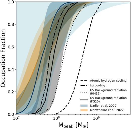
Occupation fraction as a function of the peak halo mass. The black curves, with different line styles, correspond to the predictions from our model incorporating various physical processes. Specifically, the dashed line corresponds to the model incorporating only atomic hydrogen cooling, while the dotted–dashed line represents the model incorporating both atomic and molecular hydrogen cooling (but no UV background radiation). The dotted line corresponds to the model including molecular hydrogen cooling and the UV background radiation prescription of HM12. The black curve with a shaded grey region corresponds to the model including molecular hydrogen cooling and the UV background radiation prescription of FG20. The grey-shaded region indicates a 40 per cent uncertainty in estimating the peak masses from our simulation. Additionally, the blue curve, along with the dark- and light-shaded blue regions, corresponds to the predictions by Nadler et al. (2020), while the orange curve, along with the dark- and light-shaded orange regions, corresponds to the predictions by Manwadkar & Kravtsov (2022).
Furthermore, we investigate the effects of incorporating two different background radiation models, HM12 and FG20, as described in Section 2.2. The inclusion of UV background radiation suppresses the formation of H2 in low-mass haloes and so has an influence on the formation of dwarf galaxies, resulting in a shift of the occupation fraction predictions towards higher masses. The main difference between the two UV background models lies in the chosen redshift of reionization, after which UV background radiation suppresses H2 formation in low-mass haloes. In the case of HM12, characterized by an earlier reionization redshift, we observe an earlier suppression of ultrafaint galaxy formation, thereby elevating the threshold for formation of galaxies in the occupation fraction results. We have confirmed that this result is almost entirely due to the difference in reionization redshifts between the FG20 and HM12 models, rather than, for example, the spectral distribution of UV radiation. It is worth noting that effects of inhomogeneous reionization have not been explicitly considered in our model. Previous studies have shown that these inhomogeneities may lead to varying reionization times for low-mass haloes in diverse environments (Katz et al. 2020; Ocvirk et al. 2021), potentially introducing scatter in the predictions for occupation fractions.
In order to validate our results and provide a comprehensive comparison, we compare our findings with two independent studies. First, we considered the forward-modelling framework for MW satellites presented by Nadler et al. (2020). Their model extends the abundance-matching framework (Wechsler & Tinker 2018) into the dwarf galaxy regime by parametrizing the galaxy–halo connection – including the faint-end slope of the luminosity function, the galaxy–halo size relation, the scatter in galaxy luminosity and size, and the disruption of subhaloes due to baryonic effects (Nadler et al. 2018, 2019) – and constraining these parameters using recent MW satellite observations. In particular, Nadler et al. (2020) focused on MW satellites detected in photometric data from DES and PS1, which together cover a significant portion of the high Galactic latitude sky, including the contribution of satellites originally associated with the LMC. Importantly, they incorporated position-dependent observational selection effects that accurately represented satellite searches in imaging data from surveys such as DES and PS1. In our comparisons, we utilized their posterior on the galaxy occupation fraction, where the dark and light colors in Fig. 2 correspond to the 1σ and 2σ confidence intervals, respectively, and the median is represented by the blue curve. We find that our most realistic model which incorporates H2 cooling and utilizes the UV background radiation prescription from FG20, lies within the 2σ uncertainty of the occupation fraction inferred from observations by Nadler et al. (2020).
Additionally, we examined the results obtained from the regulator-type modelling technique introduced in Kravtsov & Manwadkar (2022) and employed by Manwadkar & Kravtsov (2022) to model the MW satellite population. This approach allowed for an exploration of the luminosity function by forward modelling observations of the population of dwarf galaxies while accounting for observational biases in surveys through their respective selection functions. Furthermore, they incorporated current constraints on the MW halo mass and the presence of the LMC. In our analysis, we utilized the shaded orange region on the plot, where the dark and light colours represent the 1σ and 2σ dispersions, respectively, and the median is indicated by the orange curve.
By comparing our results with these complementary approaches, we find agreement within the 2σ dispersion range of the respective results. However, based on the median of our findings, we estimated that the peak mass above which 50 per cent of the haloes host a luminous component is approximately a factor of 2 higher than the predictions by Nadler et al. (2020) and Manwadkar & Kravtsov (2022).
It is important to highlight that galacticus does not currently account for any pre-infall mass loss from haloes. Nevertheless, N-body simulations demonstrate that peak masses are typically attained before infall, as the effects of tidal stripping begin to diminish the mass to some extent prior to infall (Behroozi et al. 2014). To account for these uncertainties, we include a shaded region representing a 40 per cent uncertainty in the determination of peak masses derived from our SAM prediction. The implementation of this missing physics is currently underway (Du & Benson, in preparation) in galacticus.
As a result of this caveat, our current model likely overestimates peak masses due to the absence of accounting for pre-infall mass loss. With improved modelling in this regard, we anticipate our estimates to align more closely with these alternative models. Specifically, our estimate suggest that approximately 50 per cent of the haloes with peak masses around ∼8.9 × 10⁷ M⊙ would host a luminous component, while Nadler et al. (2020) inferred a best-fitting value of ∼4.2 × 10⁷ M⊙ and Manwadkar & Kravtsov (2022) predicted a value of ∼3.5 × 10⁷ M⊙.
Comparing these findings against occupation fraction predictions from hydrodynamical simulations targeting similar halo mass ranges reveals that these simulations consistently predict a cut-off in ‘galaxy formation’ at higher halo masses. In particular, many hydrodynamical predictions span a range of 6.5 × 10⁸–3.5 × 10⁹ M⊙ for the bound mass at which 50 per cent of haloes host galaxies, depending on the specific model configurations and reionization redshift assumptions employed (Sawala et al. 2016a; Benítez-Llambay et al. 2017; Benitez-Llambay & Frenk 2020).10 Importantly, it should be emphasized that the definition of occupation fraction in these simulations is subject to resolution limitations, and the effects of H2 cooling must also be considered. These factors notably contribute to the disparities witnessed in the results. Nevertheless, due to the inherent dissimilarities in modelling approaches, a direct comparison between our SAM model and hydrodynamical simulations is not straightforward. For example, the simulation of Agertz et al. (2020) forms a dwarf with M⋆ ≈ 3 × 10⁴ M⊙ in a halo of mass approximately 8 × 10⁸ M⊙, while the simulation of Applebaum et al. (2021) produces several galaxies in haloes in the (bound) mass range 107–109 M⊙. These simulations are therefore consistent with our model (i.e. they imply that the occupation fraction is greater than zero at these halo masses), but do not allow for a detailed characterization of the cut-off in the occupation fraction, precluding a careful comparison with our results. For a more comprehensive understanding of how diverse assumptions and models can influence the predicted occupation fraction, please refer to Appendix B.
3.1.2 Stellar mass–halo mass relation
Fig. 3 showcases the SMHM relation, which provides crucial insights into the connection between the masses of galaxies and their DM haloes. We present the median values of the SMHM relation obtained from our model, incorporating the various physical processes discussed in Section 2. Each line style corresponds to a specific combination of physics, as outlined earlier (see Section 3.1.1). Our most realistic model, which includes H2 cooling and the UV background radiation prescription from FG20, is represented by the error bars indicating the 1σ and 2σ dispersion around the median value.
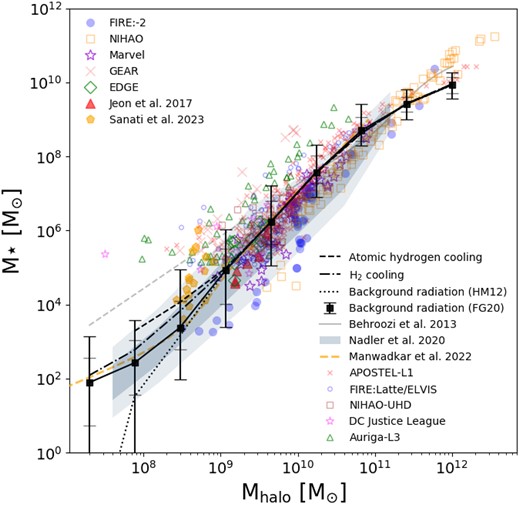
SMHM relation. Our model predictions are represented by black curves with different line styles. We compare our results to the constrained/extrapolated SMHM relation from Behroozi et al. 2013 (depicted by the grey curve/dashed grey curve), the results from Nadler et al. 2020 (illustrated by the shaded blue region), the results from Manwadkar & Kravtsov (2022, shown by the orange dashed line), and simulations of central/field dwarf galaxies in MW-like environments from various models, as well as simulations that zoom-in on individual dwarf-mass haloes (represented by different markers, please refer to the text or see fig. 2 in Sales et al. 2022 for more details).
In terms of consistency with previous studies, our estimations for the higher mass end align well with a range of simulations and the abundance matching model by Behroozi et al. (2013) as illustrated by the grey solid line. We show an extrapolation of that relation to lower mass systems in dashed grey, from which our results start to substantially deviate downwards for |$M_{\rm halo}\lt 10^9\,\, \rm M_\odot$|. Notably, we find overall agreement with recent results from Nadler et al. (2020), whose SMHM relation inferred from MW satellite observations is depicted by the shaded blue region, with darker and lighter shades corresponding to the 1σ and 2σ confidence intervals, respectively.
Additionally, we compare our results with available simulations of central/field dwarf galaxies in MW-like or Local Group-like environments (with data compiled by Sales et al. 2022).11 For these comparisons, different markers are used, as indicated in the lower right part of the plot. The marker guide includes red crosses representing APOSTLE, L1 resolution (Sawala et al. 2016b; Fattahi et al. 2016), blue open circles showing Latte and ELVIS suites (Wetzel et al. 2016; Garrison-Kimmel et al. 2019) of fire-2 simulations12 (Hopkins et al. 2018), brown squares representing NIHAO-UHD (Buck et al. 2019), pink stars showing DC Justice League (Munshi et al. 2021), green triangles representing Auriga, L3 resolution (Grand et al. 2017), while the legend in the upper left corner denotes simulations that zoom-in on individual dwarf-mass haloes. These include blue circles showing fire-2 (Wheeler et al. 2015, 2019; Fitts et al. 2017; Hopkins et al. 2018), orange squares showing NIHAO (Wang et al. 2015), purple stars showing Marvel (Munshi et al. 2021), orange crosses showing GEAR (Revaz & Jablonka 2018), green diamonds showing EDGE (Rey et al. 2019, 2020), red triangles showing work by Jeon, Besla & Bromm (2017), and orange pentagons show results by Sanati et al. (2023).
The agreement observed with various simulations provides strong support for the validity of our modelling approach. Importantly, thanks to the use of SAMs, our predictions extend to fainter regimes, surpassing the capabilities of state-of-the-art hydrodynamical simulations. Overall, our different models comparing the effect of including various physics remain consistent with each other within the 2σ dispersion in the SMHM relation. However, some deviations are observed in the ultrafaint regime, where the model incorporating H2 cooling and UV background radiation from FG20 produces the best results in terms of agreement with previous works. It is worth noting that our model slightly underpredicts the stellar mass content in the central galaxy (MW analog). None the less, the median value captures the lower end of stellar mass predictions for this halo mass range.
The SMHM relation predicted by galacticus unveils some intriguing features that align with findings from hydrodynamical simulations, such as the mass-dependent scatter in the SMHM relation, which exhibits an increasing trend around the median in the ultrafaint regime. This behaviour seems to be influenced by the impact of formation histories, particularly the duration of star formation prior to reionization, directly affecting the stellar mass content at low redshifts (Rey et al. 2019; Munshi et al. 2021). Another interesting prediction emerges in the ultrafaint regime for Mhalo < 109 M⊙ (corresponding to M⋆ < 105 M⊙), where the power-law relation in the SMHM appears to undergo a break. Remarkably, this feature appears to correlate with the dominance of H2 cooling and is further amplified by the effects of UV background radiation, specifically the time of reionization. These predictions are consistent with the SMHM relation obtained from forward modelling results by Manwadkar & Kravtsov (2022; depicted by the dashed orange line in Fig. 3), although the position of the break in this study reflects the inefficiency of supernova-driven winds in the smallest galaxies.
3.1.3 Luminosity function
Fig. 4 demonstrates our model’s predictions for the luminosity function of the MW satellite population. To ensure consistency with conducted observations, we impose two selection criteria: satellites must reside within a distance of 300 kpc from the host halo’s centre, and they should have a minimum half-light radius of rh > 10 pc. The error bars on the plot represent the 1σ and 2σ dispersion due to host-to-host scatter (across a range of halo masses). Our most accurate model predicts a total of |$300 ^{+75} _{-99}$| (|$300 ^{+166} _{-170}$|) satellites with an absolute V-band magnitude (MV) less than 0, for 1σ (2σ) dispersion.

The luminosity function of MW satellites satisfying the criteria of MV < 0, r1/2 > 10 pc, and a maximum distance of 300 kpc from the MW. Our model’s predictions, represented by black curves with distinct line styles, are compared to observational data for all known MW satellites (light red curve) and the estimate derived in Drlica-Wagner et al. (2020, maroon curve), which corrects for observational data incompleteness. Additionally, we present the results from simulations by Nadler et al. (2020, blue-shaded region), Manwadkar & Kravtsov (2022, orange-shaded region), and hydrodynamic simulations of the Local Group using the fire feedback prescription (pink-shaded region) by Garrison-Kimmel et al. (2019).
By examining our models incorporating various physics components (similar line styles as Figs 2 and 3), we discern their impact on the resulting luminosity function. Notably, the inclusion of H2 cooling leads to a considerable increase in the number of predicted ultrafaint satellites, surpassing a factor of > 3, while the incorporation of UV background radiation serves to flatten the luminosity function at the ultrafaint end.
To assess the agreement with observational data, we compare our predictions with the luminosity function of all known MW satellites (light red curve) and the DES + PS1 data (from Drlica-Wagner et al. 2020), corrected for observational incompleteness (maroon line). It is important to note that the light red curve exhibits a more pronounced flattening at the ultrafaint end due to the incompleteness in the observations. In contrast, our results closely capture the rise predicted in the weighted DES + PS1 data (refer to Drlica-Wagner et al. 2020 for details of estimation), with the total number of satellites falling within the 2σ dispersion.
Examining the higher end of the luminosity function, we find agreement (within the 2σ dispersion) between our model and observational results (although we do not constrain our model to produce analogues of the LMC and SMC in all cases). However, it is worth emphasizing that the weighted DES + PS1 results do not encompass the LMC, SMC, and Sagittarius, accounting for the lower values observed compared to the all-known case at the higher end.
Moreover, we juxtapose our results with previous forward modelling methods, including the work by Nadler et al. (2020, depicted by the blue-shaded region) and Manwadkar & Kravtsov (2022, illustrated by the orange-shaded region, as introduced in Section 3.1.1). Additionally, we incorporate the fire hydrodynamical simulation by Garrison-Kimmel et al. (2019), extending down to the fire resolution limit of ∼−6 mag (represented by the pink-shaded region). These systems do not explicitly include analogues of the LMC or SMC. Overall, our results demonstrate strong agreement with previous simulations and forward modelling approaches, albeit with a slight tendency to overpredict the median number of satellites. Notably, in the ultrafaint regime, discrepancies arise between observational data and various simulations; however, the simulations generally converge within the 2σ limit. Remarkably, our best-performing model closely reproduces the predicted weighted DES + PS1 data at the low-mass end of the luminosity function.
In light of the higher median predicted for the satellite luminosity function in our model compared to other studies, such as Nadler et al. (2020), it is important to consider some underlying differences of the respective models. For instance, variations in the underlying subhalo mass functions predicted by galacticus and cosmological zoom-in simulations (e.g. see fig. 10 of Nadler et al. 2023b) may account for some of the discrepancy. Additionally, the extent to which DM subhaloes are disrupted by the central galaxy could also influence the resulting luminosity functions. In our model, subhaloes are tidally stripped using the Pullen et al. (2014) prescription, including the potential of the central galaxy, while Nadler et al. (2020) apply a random-forest model trained on hydrodynamic simulations to capture this effect (Nadler et al. 2018).13 Importantly, our main results are robust in the sense that our predictions for the occupation fraction and SMHM relation do not change if we restrict to the subset of merger trees that produce luminosity functions similar to Nadler et al. (2020). We leave direct calibration of our model based on forward modelling the observed MW satellite population to future work.
3.2 Dwarf population
In this study, we utilize the optimal model presented in Section 2, which incorporates the physics of molecular hydrogen cooling, UV background radiation, and IGM metallicity. Our aim is to predict properties of the dwarf galaxy population and compare these to existing observations14 and simulations.
3.2.1 Mass–metallicity relation
The metallicity of a galaxy is commonly quantified by the iron to hydrogen abundance ratio ([Fe/H]). As shown in Fig. 5, we present the mean stellar [Fe/H]15 as a function of stellar mass (M⋆) for our simulation. The black curve represents the median value, while the black and grey error bars denote the 1σ and 2σ dispersions, respectively. To validate our results, we compare them with observations of dwarf galaxies located within a 300 kpc radius of the MW (illustrated by red markers). The observations indicate the presence of a metallicity plateau around [Fe/H]∼−2.5, which is reproduced well by our simulation incorporating the IGM metallicity model.
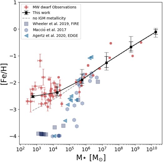
Stellar mass–metallicity relation for galaxies. The black curve, along with the black and grey error bars, represents the median value, and the 1σ and 2σ dispersions, respectively, derived from our simulation’s predictions. The grey dashed line represents the predictions of our model without the IGM metallicity included. Blue markers indicate results from hydrodynamical simulations (Wheeler et al. 2019: blue squares; Macciò et al. 2017: blue hexagon; Agertz et al. 2020: by blue triangles). Red markers with error bars depict the observational results for dwarf galaxies located within 300 kpc of the MW, compiled primarily from studies by Drlica-Wagner et al. (2020), Simon (2019), and McConnachie (2012).
Interestingly, the mass–metallicity relation for the very low-mass satellites appears to be strongly influenced by the evolution of IGM metallicity as a function of redshift. This influence becomes apparent when comparing the black curve, which includes IGM metallicity in our model, with the dashed grey curve, where the IGM metallicity is excluded, and which shows a power-law extension to low masses with no plateau.16 (The inclusion of IGM metallicity significantly affects the predicted metallicities of these satellites – essentially setting a floor in metallicity corresponding to the metallicity of the IGM gas accreted at the time at which the galaxy formed – highlighting the importance of the surrounding cosmic environment in shaping their chemical enrichment history.) When comparing our findings to zoom-in hydrodynamical simulations (such as those conducted by Agertz et al. 2020; Wheeler et al. 2019; Macciò et al. 2017), we find that these simulations tend to predict near-primordial abundances for objects with stellar masses below 105 M⊙. However, it is important to note that the examples presented in this study do not have a large cosmological environment and thus are not enriched by nearby sources (for a comprehensive comparison with recent simulation predictions refer to fig. 1 in Sanati et al. 2023). The implications of this lack of enrichment (in hydrodynamic simulations) remain uncertain and necessitate further investigation.
Recent studies have considered a few possible self-consistent avenues to populate the plateau in [Fe/H] at the faintest end of the mass–metallicity relation. The study by Prgomet et al. (2022), using the adaptive mesh refinement method, studied the effect of varying the IMF on the evolution of an ultrafaint dwarf. In this framework, at low gas metallicities, the IMF of newborn stellar populations becomes top-heavy, increasing the efficiency of supernova and photoionization feedback in regulating star formation. The increase in the feedback budget is none the less met by increased metal production from more numerous massive stars, leading to nearly constant iron content at z = 0 that is consistent with the results achieved from our model (for their case at a stellar mass of M⋆ = 103 M⊙, the typical metallicity is [Fe/H] ∼−2.5). Additionally, the study by Sanati et al. (2023), running zoom-in chemodynamical simulations of multiple haloes and including models that account for the first generations of metal-free stars (Pop III), demonstrate an increase in the global metallicity of ultrafaints, although these are insufficient to resolve the tension with observations (see their fig. 6).
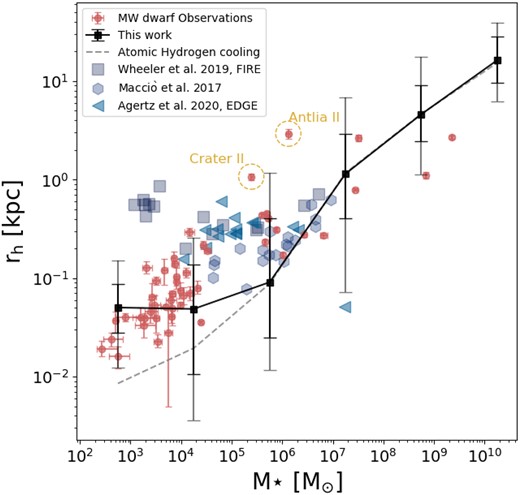
The size (projected half stellar mass radius)–stellar mass relation for dwarf galaxies. The black curve, along with the black and grey error bars, represents the median value, and the 1σ and 2σ dispersions, respectively, derived from our simulation’s predictions. The grey dashed line represents the predictions of our model only including atomic hydrogen cooling. Blue markers demonstrate results from hydrodynamical simulations (Wheeler et al. 2019: blue squares; Macciò et al. 2017: blue hexagon; Agertz et al. 2020: blue triangles). Red markers with error bars depict the observational results for dwarf galaxies located within 300 kpc of the MW, compiled primarily from studies by Drlica-Wagner et al. (2020), Simon (2019), and McConnachie (2012).
Several studies have examined the effect of different feedback processes on shaping the dwarf population (see e.g. Lu et al. 2017; Agertz et al. 2020; Smith et al. 2021). In this context, the work by Lu et al. (2017) using an SAM provides valuable insights. Their findings shed light on the connection between preventive and ejective feedback mechanisms and the stellar mass function and mass–metallicity relation of MW dwarf galaxies. Where preventive feedback acts to inhibit baryons from accreting onto galaxies, and in the realm of low-mass haloes, a commonly employed form of preventive feedback in SAMs is photoionization heating. This mechanism effectively reduces radiative cooling and mass accretion in low-mass haloes, thereby influencing the evolution of these galaxies. On the other hand, ejective feedback processes involve the expulsion of baryons from the galaxy into the IGM, often characterized by the presence of outflows. These mechanisms play a significant role in shaping the gas content and subsequent star formation in dwarf galaxies. By incorporating both preventive and ejective feedback in their model, Lu et al. (2017) demonstrate the ability to simultaneously match the observed stellar mass function and the mass–metallicity relation. Moreover, they highlight the importance of considering a redshift dependence for preventive feedback, although the precise nature of this dependence remains largely uncertain.
Building upon the insights from Lu et al. (2017), our results further support the notion that the mass–metallicity relation for low-mass dwarfs is intricately linked to the interplay between feedback processes and the enrichment of the surrounding environment (i.e. enrichment of the IGM). We acknowledge that our approach is not self-consistent, as we do not explicitly account for the metal outflows from our galaxies and their mixing into the IGM. However, the inclusion of IGM metallicity in our model becomes imperative to achieve consistency with observational data, as demonstrated by our agreement with observations.
Another study, conducted by Pandya et al. (2021), showcases that the mass-loading factors for winds in dwarf galaxies can be large (i.e. ≫1; as evident from their fig. 7), and these winds are responsible for carrying away a significant portion of the produced metals. They also reveal that higher mass galaxies exhibit substantially lower mass-loading factors for their winds, along with lower metal-loading factors. This finding suggests that dwarf galaxies may play a substantial role in enriching the IGM. Given these compelling facts, our SAM approach has the potential to allow us to resolve the dwarf galaxies and accurately predict IGM metal enrichment. Simultaneously, our SAM enables us to model the massive haloes, which actively accrete gas from the enriched IGM, facilitating a comprehensive understanding of the intricate interplay between galaxies and their surrounding environment.
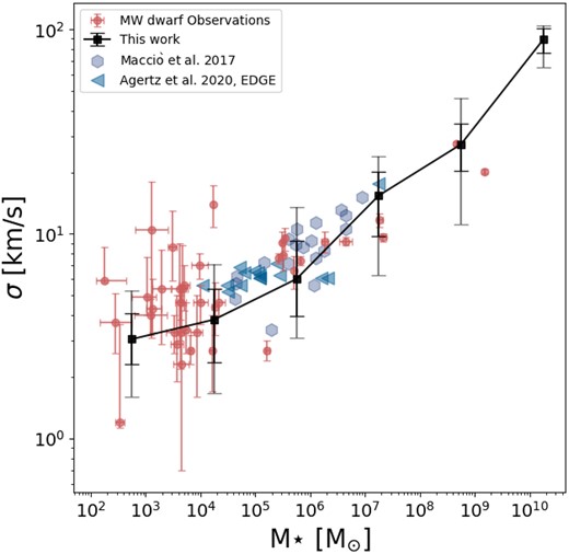
The 1D line-of-sight velocity dispersion (measured at the half stellar mass radius)–stellar mass relation. The black curve, along with the black and grey error bars, represents the median value, and the 1σ and 2σ dispersions, respectively, derived from our simulation’s predictions. The hydrodynamical simulation results are shown by blue markers (Macciò et al. (2017, blue hexagons and Agertz et al. (2020 blue triangles). The red markers with error bars depict the observational results for dwarf galaxies located within 300 kpc of the MW, compiled primarily from studies by Drlica-Wagner et al. (2020), Simon (2019), and McConnachie (2012). Our results demonstrate agreement with the velocity dispersion–mass relation in higher mass galaxies, while indicating lower median predictions for galaxies with stellar masses below 105 M⊙.
3.2.2 Size–mass relation
We measure the projected half-mass radius (rh) for all galaxies in our sample and plot it against the predicted stellar masses. As depicted in Fig. 6, the black curve represents the median value, while the black and grey error bars indicate the 1σ and 2σ dispersions, respectively. Our predictions successfully capture the size–mass relation for the majority of observed galaxies (depicted by red markers) within the 2σ range of our sample. Interestingly, we find that systems resembling Antlia II and Crater II are sometimes predicted by our model, although they lie far away from the median of the relation predicted by the model. Such galaxies correspond to the high angular momentum tail of the distribution of galaxy angular momenta – we will discuss the relation between size and angular momentum in more detail below. When comparing our results to hydrodynamical simulations, we generally agree with their best predictions above the ∼ 105 M⊙ limit, with the exception of a few extreme cases (e.g. the outlier presented by Agertz et al. 2020, where no feedback is included).
In our simulation, sizes are determined by the specific angular momentum content of stars and gas, as described by the equation:
where vh is the rotational speed at the half-mass radius, rh is the half-mass radius, and Mh is the total mass content within the half-mass radius. Given that intermediate- and low-mass dwarfs are predominantly DM-dominated, and we have a reasonably accurate SMHM relation and a correctly modelled occupation fraction distribution, it is likely that the DM mass estimate is accurate. If we aim to explain the changes of slope in the size–mass relation of galaxies, the most apparent approach would be to look at the changes in the angular momentum content.
The angular momentum is primarily determined by the angular momentum of the gas in the halo during its formation, and subsequently, by the fraction of that angular momentum that is transferred into the galaxy through cooling and gas accretion, as well as the fraction that is expelled by outflows. These factors encompass a certain level of uncertainty. In our current model, we address the inefficiencies of atomic hydrogen cooling by incorporating H2 cooling. Specifically, for temperatures below 104 K, corresponding to halo masses around 109 M⊙, which host galaxies with stellar mass components ranging from 104 to 105 M⊙, the dominant cooling mechanism becomes H2 cooling. Additionally, we include the UV background radiation model by FG20, which suppresses gas accretion. From Fig. 3, we observe that its effects are maximized for dwarfs with stellar masses below 105 M⊙. The overall effect becomes evident when comparing the black solid line representing our optimal model to the dashed grey line, where only atomic hydrogen cooling is present and no UV background radiation was used. These results suggest that variations in cooling mechanisms along with gas accretion suppression can account for the observed changes in the slope at these particular mass scales. TAR
3.2.3 Velocity dispersion—mass relation
We measure the 1D line-of-sight velocity dispersions at the half stellar mass radius for all galaxies in our sample and plot them against the predicted stellar masses. In Fig. 7, similar to Fig. 6, the black curve represents the median value, while the black and grey error bars indicate the 1σ and 2σ dispersions, respectively. Our predictions successfully reproduce the velocity dispersion–mass relation for observed galaxies within the 2σ limit of our sample (all the observational data are represented by red markers). We compared our results with hydrodynamical simulations by Macciò et al. (2017) and Agertz et al. (2020), shown by blue markers, finding general agreement within the 2σ dispersion limit.
It is worth noting that our model does not fully capture the observed scatter in 1D velocity dispersions at the lower mass end. Several potential reasons may explain this. First, it is possible that our current model does not incorporate all the relevant physical processes that govern the ultrafaint regime. The intricate dynamics and feedback mechanisms specific to these low-mass galaxies could play a significant role in shaping their velocity dispersions. Secondly, observational limitations introduce additional uncertainties in our measurements. Factors such as contamination from foreground stars in the MW and the influence of binary stars within the sample of stars from the ultrafaint dwarfs (see Simon 2019 for further details) could contribute to the observed large dispersions.
We would like to highlight that, given the observational uncertainties, our model’s predictions align well with the data, providing consistency without necessitating the inclusion of core formation. However, it is crucial to emphasize that these observational uncertainties also mean that we cannot conclusively rule out the possibility of core formation being present. This highlights the need for improved and more precise measurements in order to better understand and constrain the underlying physical processes. Additionally, our model’s success in matching the velocity dispersion, combined with accurate predictions of the occupation fraction, suggests that it is effectively free of the too-big-to-fail problem (Boylan-Kolchin, Bullock & Kaplinghat 2011).
3.3 Mass function predictions for various halo masses
Once calibrated, we can use our model to make predictions on the abundance of satellite galaxies for host systems with varying virial masses. In Fig. 8, we depict the cumulative stellar mass functions for subhaloes associated with various haloes of different masses, specifically showcasing satellites with stellar masses (M⋆) greater than |$10^2 \rm \mathrm{M}_\odot$| and half-mass radius (r1/2) larger than 10 pc. The dark and light shaded grey regions represent the 1σ and 2σ dispersions, respectively, while the black line shows the median of the results. For comparison, the red curve represents available observational results,17 and the blue dashed and dotted curves represent the results from the abundance matching study by Santos-Santos et al. (2022). The blue dotted line corresponds to their ‘power-law’ model, assuming a power-law relation for the M⋆–Vmax relation, while the blue dashed curve corresponds to their ‘cut-off’ model, assuming a cut-off in this relation.
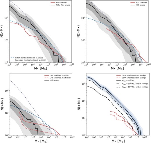
Predictions of our model for the cumulative stellar mass function of satellites. The black curve represents the median of our results, while the light- and dark-shaded regions indicate the 1σ and 2σ dispersions, respectively. Observational constraints, if available, are shown by the red curves. The dashed and dotted blue lines correspond to the ‘Cutoff’ and ‘PowerLaw’ models from Santos-Santos et al. (2022), allowing for a comparison with their results. Each panel displays our results for a different halo mass: the top left panel corresponds to the MW-analogue halo, the top right panel to the M31-analogue halo, the bottom left panel to the LMC-analogue halo, and the bottom right panel to a group-size halo with a mass of 1013 M⊙.
In the top left panel, we present our results for the MW analogue. We ran 100 haloes with virial masses ranging from 7 × 10¹¹ to |$1.9 \times 10^{12} \rm \mathrm{M}_\odot$|, in agreement with the current available mass constraints (Wang et al. 2020; Callingham et al. 2019). Our results show a reasonable agreement with the observations for the stellar masses of larger satellites (within 300 kpc from the MW). However, for the lower mass range, the discrepancy between our results and the observations becomes more prominent. This discrepancy could be partially attributed to incompleteness in the observational results, as we discussed in Section 3.1.3, where estimations for corrections in the observational data predict much higher values for the number of MW satellites (Tollerud et al. 2008; Drlica-Wagner et al. 2020). Overall, our model suggests that only ∼20 per cent of the MW satellites with MV < 0 have been discovered.
Comparing with the results of Santos-Santos et al. (2022), we find reasonable agreement up to a stellar mass of |$10^5 \rm \mathrm{M}_\odot$| for the satellites, and our results deviate from their predictions in the ultrafaint regime. Notably, the slope of our results in this regime shows better agreement with their power-law model, although the total predicted number of haloes is a factor of ∼2 lower. It is worth mentioning that this slope was only achieved by including the effects of H2 cooling, as our model with only atomic hydrogen physics shows flatter slopes, in better agreement with their cut-off model (see Fig. 4 for comparison of our models).
The top right panel presents our results for the M31 analogue. Similar to the MW case, we ran 100 realizations of a halo with a mass of |$1.8 \pm 0.5 \times 10^{12} \rm \mathrm{M}_\odot$|, in agreement with M31 mass constraints (from Shull 2014; Diaz et al. 2014; Karachentsev & Kudrya 2014; Benisty et al. 2022). Our results show agreement with the observations within the 2σ limit (albeit we get lower results for the higher mass end), although the surveyed population in M31 does not extend as deeply as our predictions show. Similar to the MW case, we observe agreement with Santos-Santos et al.’s (2022) results in the higher mass regime, while in the ultrafaint regime, our model predicts results closer to their power-law model. It is worth mentioning that their models assume an occupation fraction of 1 for their haloes, whereas we found in Section 3.1.1 that only a fraction of our haloes with peak masses below |$2 \times 10^8 \rm \mathrm{M}_\odot$| host a luminous component.
The bottom left panel shows our results for the LMC-analogue halo. We present the mass function results for satellite stellar masses based on 100 realizations of hosts with halo masses of 1.88 ± 0.35 × 10¹¹ M⊙ (Shipp et al. 2021). Our findings estimate that an isolated LMC analogue is expected to have approximately 33|$^{+14}_{-12}$| satellites (for 1σ dispersion) with stellar masses above 102 M⊙ and r1/2 larger than 10 pc, lying within the halo’s virial radius. Most of the realizations indicate that satellites have stellar masses below 4 × 10⁶ M⊙, and the likelihood of generating an SMC within the virial radius is relatively low.
We then compare these results with the satellites associated with the LMC based on the kinematic analysis conducted by Santos-Santos et al. (2021). According to their analysis, 11 of the MW satellites appear to have some connection with the LMC (‘possible’), and from those, 7 show firm association (‘most likely’). Our results seem to underpredict the number of higher mass subhaloes, while overpredicting the number of currently observed ultrafaint satellites. Apart from considering the effects of observational incompleteness, other factors may be at play here. First, we do not constrain our LMC analogues to have any high-mass satellites such as the SMC. The occurrence of reproducing such a massive companion for the LMC in our model is probabilistically low, as only 1 such satellite was produced in our 100 realizations of the LMC, and it is located at a distance of approximately 140 kpc from the LMC analogue (beyond the virial radius of this halo/radius of approximately 100 kpc where we measure the associated satellites). Additionally, we are running our LMC analogues as isolated haloes and not in association with a larger halo such as the MW. The presence of a larger gravitational potential can more effectively disrupt the ultrafaint satellites, thereby decreasing the number of predicted satellites associated with the LMC.
Comparing with the results from Nadler et al. (2020), they predict 48 ± 8 LMC-associated satellites with MV < 0 mag and r1/2 > 10 pc, approximately consistent with our predictions of 33|$^{+14}_{-12}$| for 1σ (33|$^{+28}_{-26}$| for 2σ). This is also in reasonable agreement with the ∼70 satellites with −7 < MV < −1 predicted by Jethwa, Erkal & Belokurov (2016) via dynamical modelling of the Magellanic Cloud satellite population. Additionally, our predictions can be compared with the work of Dooley et al. (2017), who explored the satellite population of LMC-like hosts using several abundance-matching models and estimated ∼8–15 dwarf satellites with |$M_* \ge 10^3 \rm \mathrm{M}_\odot$| within a 50 kpc radius of their hosts. Applying similar selection criteria to our model results gives us an estimation of 6|$^{+6}_{-4}$|. Furthermore, our results align well with the study by Jahn et al. (2019), where they used five zoom-in simulations of LMC-mass hosts (with halo masses ranging from 1 × 10¹¹ to 3 × 10¹¹ M⊙) run with the fire galaxy formation code, predicting ∼ 5–10 ultrafaint companions for their LMC-mass systems that have stellar masses above 104 M⊙ (compared to our estimation of 6|$^{+5}_{-4}$| for 1σ dispersion). However, it is worth noting that our stellar mass function is steeper than their results.
The bottom right panel illustrates our model’s prediction for the satellite stellar mass function of subhaloes within group-sized haloes. These results are based on 100 realizations of a host halo with a mass of |$10^{13} \, \mathrm{M}_{\odot }$|. The shaded region in this plot is depicted in a distinct colour as it differs from the other panels. In this case, the dispersion only represents variations resulting from constructing merger trees for the exact same halo mass, while in other panels, we include a range of masses for the haloes, leading to a larger halo-to-halo scatter.
Regarding the predicted stellar mass function for the satellites, we find more massive satellites compared to those in the MW and M31, along with a larger number of total subhaloes (with r1/2 > 10 pc) within a radius of 450 kpc from the central galaxy (or the estimated virial radius). This trend is consistent with expectations for a halo with a larger virial mass. As a candidate in the nearby Universe, we compare our results to Centaurus A (Cen A for short) with virial mass estimations ranging from 6.4 × 10¹² to 1.8 × 10¹³ M⊙ (Karachentsev et al. 2007; van den Bergh 2000). The V-band magnitudes of Cen A’s satellites were compiled from Crnojević et al. (2019).
The study by Crnojević et al. (2019) covers approximately half of the virial radius estimated for Cen A and includes satellites down to MV = −7.8 (equivalent to a stellar mass of approximately 105 M⊙). Additionally, Crnojević et al. (2019) provide results from earlier studies of Cen A (Sharina et al. 2008; Karachentsev, Makarov & Kaisina 2013), which target a wider region around the central galaxy, albeit with a lower limiting magnitude. Since the observational surveys each cover part of this group, we have adjusted the radius within which we make the comparison accordingly. Our model predictions depicted by the black dashed line, corresponds to satellite mass function within a radius of 150 kpc from the central galaxy. This selection mirrors the observational results with the same cuts, as shown by the red dashed line. Additionally, our results shown by the dashed–dotted line represent the satellite mass function within 300 kpc from the central galaxy, which can be compared to the observational data with similar cuts, as indicated by the red line.
Our results align well with the slope of the observational satellite stellar mass function at the higher mass end, although the exact number of predicted satellites is slightly higher. This can be interpreted as our results favoring a virial mass for Cen A close to the lower end of the current estimates, as number of satellites tend to scale on host halo mass. In any case, if we assume that a 1013 M⊙ halo is a good representation of this system, our results suggest that a factor of ∼5–7 satellites with stellar masses above 105 M⊙ are waiting to be discovered in this system. Additionally, a study by Weerasooriya et al. 2023b (in preparation), utilizing the model outlined in Weerasooriya et al. (2023a), has also examined the Cen A system. Their prediction for the total count of satellites with MV magnitudes lower than −7.4 (equivalent to stellar masses around 105 M⊙) amounts to median number of 50. While the median is slightly lower than their compiled observational data for satellites of Cen A within 150 kpc,18 the predicted distribution of the number of satellites still falls within the observed range. These results are marginally lower than our predictions below MV ∼ −10.
4 CONCLUSIONS
In this study-, we have modified the galacticus SAM to incorporate key physical processes relevant to the formation of dwarf galaxies, and utilized that model to explore predictions for the galaxy–halo connection and the properties of the dwarf galaxy population of the MW. Through the inclusion of essential physical processes such as IGM metallicity, H2 cooling, and UV background radiation, coupled with the fine-tuning of various parameters, we have achieved significant success in replicating several characteristics observed in the dwarf galaxy population.
First and foremost, we find that our model with updated physics is able to reproduce the inferred SMHM relation while simultaneously reproducing the main physical properties of the dwarf galaxy population. This finding underscores the robustness of our model and its ability to capture the relationship between the stellar content and the underlying DM haloes. Furthermore, our results demonstrate that the inclusion of H2 cooling and a UV background radiation (prescribed by FG20), motivated by recent observational constraints, is crucial to achieving an occupation fraction consistent with previous inferences. Our study reveals that the fraction of subhaloes hosting galaxies with an absolute V-band magnitude less than 0 drops to 50 per cent at a halo peak mass of ∼8.9 × 10⁷ M⊙. Notably, earlier estimations based on older UV background estimates (HM12) do not yield the same level of agreement.
When examining the statistical properties of the MW dwarf population, we find broad success in reproducing key characteristics. Our predictions for the luminosity function of the MW dwarfs align well with observations once we account for the inherent halo-to-halo scatter. Remarkably, the presence of H2 cooling is vital for capturing the large number of ultrafaint dwarf galaxies, highlighting its role in driving their formation. Our model predicts a total of |$300 ^{+75} _{-99}$| satellites with an absolute V-band magnitude less than 0 within 300 kpc from our MW analogues. This number would drop down to |$91 ^{+42} _{-34}$| if we were to use our model including only the atomic hydrogen cooling. Our model of H2 formation/destruction remains quite simplistic. Plausible changes in the underlying assumptions in computing metal cooling and H2 formation/destruction under a radiation field (e.g. considering radiation from local sources, not just a mean background), could result in changes to the cooling efficiencies in small, early-forming haloes. The efficiency and relevance of H2 cooling in such haloes remain subjects of ongoing debate (refer to section 4.3.2 of the review by Klessen & Glover 2023, and references therein).
Moreover, the inclusion of IGM metallicity enables us to successfully reproduce the mass–metallicity relation without the need for preventive feedback mechanisms. Our model achieves successful agreement with the sizes and velocity dispersions of ultrafaint dwarfs.
Finally, our model successfully predicts the stellar mass function of satellites for both MW and M31 analogues. Additionally, we use our model to make predictions for the two different mass scales: LMC and Cen A analogues. Our results demonstrate a general agreement with the available observational data, emphasizing the robustness of our model in generating predictions across a broad range of halo masses. The combined functionalities of this model, along with its comprehensive approach to predicting various aspects of the dwarf population, makes it uniquely powerful for investigating the faintest galaxy population across a range of environments/halo masses.
Looking ahead, there are several exciting directions to explore. Investigating how our results are influenced by the inclusion of an LMC analogue in the MW mass haloes will provide valuable insights into the impact of satellite galaxies on the MW dwarf population, for example, following the constrained merger tree methodology presented in Nadler et al. (2023a). Furthermore, exploring alternative non-CDM models, such as self-interacting DM, will allow us to gauge the extent to which observations of dwarfs can inform our understanding of the nature of DM itself.
ACKNOWLEDGEMENTS
We gratefully acknowledge the contributions of several individuals who supported this research. Special thanks to our referee, Martin Rey, whose valuable suggestions greatly improved this work. We would like to express our appreciation to Isabel Santos-Santos for generously providing the valuable data from (Santos-Santos et al. 2022). We are also thankful to Ana Bonaca, Viraj Manwadkar, Yves Revaz, Risa Wechsler, and Fakhri S. Zahedy for engaging in insightful conversations and offering valuable input throughout the course of this study. NA and LVS acknowledge financial support from NSF-CAREER-1945310 and NSF-AST-2107993 grants. NA would like to acknowledge the support provided by the UCR-Carnegie Graduate Fellowship. The computations presented here were conducted through Carnegie’s partnership in the Resnick High Performance Computing Center, a facility supported by Resnick Sustainability Institute at the California Institute of Technology. Additional computations were carried out on resources made available through a generous grant from the Ahmanson Foundation.
DATA AVAILABILITY
The SAM model utilized in this project is openly accessible and can be accessed at the following link: https://github.com/galacticusorg/galacticus/. Researchers and interested parties can freely explore and utilize the SAM model to replicate and build upon the findings presented in this study.
Footnotes
We refer the reader to Crnojević & Mutlu-Pakdil (2021) for examples of discovered dwarfs in each survey.
The specific version used in this work is publicly available at https://github.com/galacticusorg/galacticus.
While this is true for the model presented in this work, we caution readers that the outcomes may be sensitive to the underlying assumptions in computing metal cooling and H2 formation/destruction in the presence of a radiation field. For instance, a comparison of our cooling efficiencies with Bialy & Sternberg (2019) reveals overall agreement at the typical densities of our haloes, although they emphasize the impact of the surrounding radiation field, particularly the susceptibility of H2 to destruction by the far-UV radiation (see their fig. 7, top panels), and the strong density dependence in the contribution of H2 to cooling. The efficiency of H2 cooling in small, early-forming haloes, considering photodissociation through Lyman–Werner radiation in the presence of H2 self-shielding, remains a debated topic in the literature (see section 4.3.2 of the review by Klessen & Glover 2023, and references therein). In general, the actual efficiency and relevance of H2 cooling in small, early-forming haloes are subjects of ongoing debate.
galacticus implements the ram pressure stripping model of Font et al. (2008) as described in Benson et al. (2015). As the mass of the CGM in a subhalo is reduced due to the effects of ram pressure stripping from the CGM of its host halo, we assume that this mass is removed in spherical shells from the subhalo CGM, starting at the outer edge, rCGM. In this way, the outer edge, rCGM, decreases over time as ram pressure stripping proceeds.
Dynamical time here is defined as τdyn = |$\sqrt{r_\mathrm{v}^3/\mathrm{G} M_\mathrm{v}}$|, where rv and Mv are virial radius and virial mass of the halo, respectively.
The decision to use a coarse grid was primarily due to the computational expense associated with more extensive analyses, such as MCMC, which would be necessary for a comprehensive exploration of all free parameters across all models in this SAM. Given the computational limitations, we focused on finding the optimum values for the free parameters in the IGM metallicity model. However, it is important to acknowledge that the coarse grid search resulted in insufficient information to calculate a meaningful theoretical uncertainty for these parameters. Despite this limitation, we have ensured that the optimization process has good coverage of the available parameter space to the best extent possible under the computational constraints.
It is essential to treat the IGM metallicity values from Ucci et al. (2023) as a lower limit since their method assumes that ejected metals are homogeneously dispersed into the entire simulation box when calculating ZIGM.
Note that the work by Benitez-Llambay & Frenk (2020) analyse results based on both hydrodynamical and semi-analytical simulations.
It is important to acknowledge that discrepancies might arise when comparing isolated dwarfs from hydrodynamical simulations due to potential variations in the definition of halo mass. Our model specifically focuses on dwarf satellites within MW systems. However, the purpose here is to emphasize the general concurrence between the outcomes of our model and the findings of existing simulations.
The latest version of fire simulation (fire-3) shows even better agreement with our predictions (see fig. 9 in Hopkins et al. 2023).
We note that Hartwig et al. (2022) predict a total number of MW satellites comparable to our results without incorporating H2 cooling or accounting for tidal stripping due to the central galaxy.
In our present galacticus model, [Fe/H] is computed using the instantaneous recycling approximation, and the assumption of Solar abundance ratios.
With no IGM metallicity, the metallicities of our galaxies are determined by our feedback/outflow model, which has a simple power-law dependence on halo mass, and so necessarily leads to a power-law mass–metallicity relation.
The V-band magnitudes for satellites of the MW, M31, and LMC are sourced from McConnachie’s (2012) revised compilation of Local Group dwarfs. For the Cen A system, values are extracted from Crnojević et al. (2019). Subsequently, the stellar masses are computed by employing relevant mass-to-light ratios derived from galacticus predictions specific to the respective stellar masses.
Their work encompasses a comprehensive compilation of the luminosity function for Cen A, including available observational data from Crnojević et al. (2014, 2016, 2019), Doyle et al. (2005), James et al. (2004), Karachentsev et al. (2003, 2013), Lauberts & Valentijn (1989), Müller, Jerjen & Binggeli (2015, 2017), Müller et al. (2019), Sharina et al. (2008), Taylor et al. (2016), and de Vaucouleurs et al. (1991). It is important to note that their data set includes all dwarf candidates, not exclusively confirmed cases.
This ‘unaccreted’ reservoir represents gas in the vicinity of the halo which has been unable to accrete due to thermal pressure.
In detail this is not correct, as there is also some dependence on the change in redshift across the time-step due to the dependence of virial densities on redshift. In practice, we ignore this dependence and absorb such effects into the parameter σ.
Due to computational limitations, these results are derived from simulations with only four merger trees, sampled from the same mass range as other cases. Given the negligible predicted scatter for the halo-to-halo cases, we anticipate minimal impact on the calculated median occupation fraction.
References
APPENDIX A: DETAILS ON CONSTRAINING MODEL
In this work, we utilize a model similar to that recently proposed by Weerasooriya et al. (2023), but with some differences which result from the recalibration of our model after including the physics described in Section 2. Here, we outline the parameters that need adjustment.
Cooling rate: we follow White & Frenk (1991) to account for the cooling rates based on the following expression.
where rinfall is the infall radius in the hot halo and ρ(r) is the density profile of the hot halo.
Feedback: we adopt a power-law model to parametrize the stellar feedback, treating the disc and spheroidal components separately. The outflow rate is calculated using the following equation:
Here, Voutflow is the characteristic velocity, set to 250 and 100 km s−1 for the disc and spheroid components, respectively. The tunable exponent αoutflow is set to 2 for both components. E is the rate of energy input from the stellar populations and Ecanonical is the total energy input by a canonical stellar population, normalized to 1 M⊙ after infinite time.
Reionization model: our reionization model employs a methodology similar to that introduced by Benson (2020). Specifically, we assume that the IGM is instantaneously and fully reionized at redshift z = 9.97, as determined by Hinshaw et al. (2013). This instantaneous reionization results in a rapid photoheating of the IGM to T = |$3 \times 10^{4}\, \mathrm{K}$|, followed by a cooling such that the temperature at redshift z = 0 drops to T = |$1 \times 10^{3}\, \mathrm{K}$|, resulting in an electron scattering optical depth of 0.0633 in this model.19
Accretion mode: accretion of baryonic component into haloes is computed using the filtering mass prescription of Naoz & Barkana (2007). In this prescription, it is assumed that the gas mass content of the haloes is given by:
where MF is the filtering mass, as first introduced by Gnedin (2000, here defined following Naoz & Barkana 2007), M200b is the halo mass defined by a density threshold of 200 times the mean background density, and Ωb and ΩM are baryon and total matter densities as a fraction of the critical density, and
The accretion rate onto the halo is therefore assumed to be
However, in practice, three assumptions are violated. First, the filtering mass is not constant in time; secondly, Mtotal does not always correspond to M200b; and thirdly, the growth of haloes occurs through both smooth accretion and merging of smaller haloes. As a result, the mass fraction in the halo will differ from f(M200b/MF). To address this issue, it is additionally assumed that mass flows from the hot halo reservoir to an ‘unaccreted’ mass reservoir20 at a rate:
where αadjust = 0.3 is chosen to ensure that the relation between gas mass and halo mass in equation (A3) is approximately maintained, τdyn is the dynamical time-scale, Munaccreted is the mass in the unaccreted reservoir, and faccreted. By making these adjustments in the model, the effects of the increased gas pressure in the IGM on accretion into the CGM are accounted for.
Angular momentum: to track the angular momentum content of haloes (and their constituent gas) we adopt the random-walk model first proposed by Vitvitska et al. (2002) and developed further by Benson, Behrens & Lu (2020, readers are encouraged to consult this paper for more detailed information) which predicts the spins of DM haloes from their merger histories. According to this model, the acquisition of angular momentum by haloes occurs through the cumulative effects of subhalo accretion. By incorporating this angular momentum prescription, we can effectively reproduce the distribution of spin parameters observed in N-body simulations (Benson et al. 2020). This approach is advantageous in accounting for the intricate processes associated with halo formation and evolution (specifically for the lower mass objects), thereby providing a more accurate representation of the dynamics and properties of the simulated haloes.
In Benson et al. (2020), the model was applied only to very well-resolved haloes. Since, in this work, we want to explore galaxy formation in very low-mass haloes – much closer to the resolution limit of the merger trees – it becomes imperative to consider the unresolved mass accretion into the haloes and the corresponding alterations in angular momentum, particularly for the lower mass range. Therefore, we include an additional stochastic contribution to the angular momentum from unresolved accretion. This represents the fact that the angular momentum vector of a halo will diffuse away from zero in a random walk even if the mean angular momentum contributed by unresolved accretion is zero. The three components of the angular momentum vector of unresolved accretion are treated as independent Wiener processes with time-dependent variance that scales as the characteristic angular momentum of the halo. Specifically, each component of the angular momentum vector obeys:
where |$\Delta J^2_\mathrm{v}$| represents the change in (the square of) the characteristic angular momentum of the halo, Jv = Mv(t)Vv(t)Rv(t), due to unresolved accretion. Here Mv(t), Vv(t), and Rv(t) are the virial mass, velocity, and radius, respectively, σ2 represents the variance in angular momentum per unit increase in |$J_\mathrm{v}^2$|, and N(0, 1) is a random variable distributed as a standard normal.
Making the approximation that the characteristic angular momentum scales in proportion to mass,21 we can write
where Mr and Mu are the resolved and unresolved mass accreted between times t1 and t2, respectively.
This model captures the idea that the increase in angular momentum from a merging event should be of order ΔMVv(t)Rv(t) (since merging haloes have velocities which scale with Vv(t) and occur at separation Rv(t)). Additionally, because this is a Wiener process the resulting distribution of Ji(t) at any given time is independent of the number of steps used to get from t = 0 to that time. (That is, the results are independent of how finely we sample the mass accretion history of each halo.) We find that σ2 = 0.001 results in reasonably good agreement between predicted and observed galaxy sizes (as discussed in more detail in Section 3.2.2).
A1 Dark matter halo evolution in galacticus
Unlike the approach taken by Weerasooriya et al. (2023), who utilized merger trees extracted from N-body simulations, this study utilizes the galacticus framework for the evolution of both the DM and baryonic components within the haloes. Here, we provide a brief overview of this process. galacticus constructs merger trees for DM haloes backwards in time using the algorithm of Cole et al. (2000), along with the modified merger rates found by Benson (2017), which were constrained to match the progenitor mass functions in the MultiDark (Klypin et al. 2016) N-body simulation suite (see here). It then evolves the properties of the haloes forward in time. When haloes merge, the more massive one becomes the host, while the smaller one becomes a subhalo orbiting within it. Subhaloes are initialized at the host’s virial radius, positioned isotropically at random, with velocities drawn from distributions predicted by cosmological simulations. In this work, we adopt parameters from Jiang et al. (2015) and best-fitting values from Benson et al. (2020). The positions and densities of subhaloes are tracked over time, accounting for dynamical friction, tidal stripping, and tidal heating until specified disruption criteria are met (Pullen et al. 2014; Yang et al. 2020). To enable rapid simulation, interactions between subhaloes are ignored (see Penarrubia & Benson 2005, for a justification of this approximation), and subhaloes are disrupted if their bound mass falls below 107 M⊙ or they pass within a distance from the host halo centre equal to 1 per cent of the host’s virial radius. For a more comprehensive explanation, refer to Yang et al. (2020), we also refer the reader to the recent comparison between galacticus predictions and Symphony simulations in Nadler et al. (2023b).
Here, we explain further the non-linear dynamical processes that govern the subhalo orbital evolution within the host halo.
Dynamical friction: causes a subhalo to decelerate as it traverses the DM particles of the host halo. This is modelled using the Chandrasekhar formula (Chandrasekhar 1943), assuming a Maxwell–Boltzmann distribution of host particles (see equation 1 in Yang et al. 2020). Which introduce our first free parameter, the ‘Coulomb logarithm (ln Λ)’.
Tidal stripping: removes mass from the subhalo that lies beyond the tidal radius (King 1962; van den Bosch et al. 2018), where the tidal force from the host exceeds the subhalo’s self-gravity. This is modelled following Zentner et al. (2005), with mass being removed outside the tidal radius over an orbital time-scale (see equation 5 in Yang et al. 2020). Our second free parameter, α, controls the strength of tidal stripping.
Tidal heating: injects energy into the subhalo through rapidly varying tidal forces, causing it to expand. This is modelled using the impulse approximation with an adiabatic correction factor and a tidal tensor time integral decay term (see equation 8 in Yang et al. 2020). The exponent γ controls the adiabatic correction term, as discussed by Gnedin & Ostriker (1999). The value of γ is somewhat uncertain, with Gnedin & Ostriker (1999) finding γ = 2.5 (which was used by Pullen et al. 2014), while theoretical considerations predict γ = 1.5 in the slow-shock regime (Gnedin & Ostriker 1999; Weinberg 1994a, b). The heating coefficient, ϵh, which accounts for the higher order heating effects, is treated as a free parameter. This model was later improved by incorporating second-order terms in the impulse approximation for tidal heating (see equation 4 in Benson & Du 2022), allowing for an accurate match to the tidal tracks observed in high-resolution N-body simulations (refer to Benson & Du 2022, for further details).
An initial calibration of these free parameters was performed by Yang et al. (2020) using an MCMC fitting workflow to thoroughly explore the parameter space with high efficiency. For the purpose of this study, we adopt ln Λ = 1.35, ϵh = 2.70, and α = 2.95. We approximate these values for the choice of γ = 1.5 (as used in the updated tidal heating model of Benson & Du 2022) by interpolating between the cases of γ = 0.0 and 2.5, using the Caterpillar simulations as calibration target.
APPENDIX B: OCCUPATION FRACTION – COMPARISON WITH HYDRODYNAMICAL SIMULATIONS
Fig. B1 shows a comparison of our occupation fraction predictions to those from several hydrodynamical simulations. At face value, our model predicts the occupation of substantially lower-mass haloes compared to simulations. The solid black line with grey shading indicates our preferred model, while lines in blue hues represent predictions from hydrodynamical simulations from Sawala et al. (2016a), Benitez-Llambay & Frenk (2020), and Munshi et al. (2021, see the legends). However, there are two main factors that complicate this comparison. First, the physics included (and its implementation) vary substantially from model to model. We have checked in detail the different physics being implemented in galacticus compared to these other simulations and conclude that the inclusion of H2 cooling, likely accounts for the majority of the difference between our predictions and those of some hydrodynamical simulations. We show in the dashed black line how our predictions would change if only atomic hydrogen cooling was included. As expected, it lowers the occupation fraction of low-mass haloes, bringing our model into closer agreement with simulations, although it still shows a somewhat higher fraction of haloes with a luminous component compared to hydrodynamical simulations.
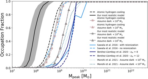
Comparison to occupation fractions predicted by hydrodynamical simulations. Solid black line with grey shading shows the result of our preferred model, while the long-dashed thick black curve indicates the median occupation fraction when not including H2 cooling. Results from Sawala et al. (2016a) and Benitez-Llambay & Frenk (2020) are presented with blue and light-blue curves. Dotted lines with blue hues illustrate results from Munshi et al. (2021). For all hydrodynamical simulations, the resolution to call a halo ‘dark’ varies between |$M_* \lt 10^4 \rm -10^5\,\, \rm M_\odot$|, as indicated by the labels. To imitate resolution effects from simulations, we apply further cuts to our preferred and no-H2 cooling models considering as ‘dark’ galaxies with |$M_* \lt 10^4\,\, \rm M_\odot$| (starred symbols) and |$M_* \lt 10^5\,\, \rm M_\odot$| (triangle symbols). Including resolution cuts, in particular |$M_* \lt 10^5\,\, \rm M_\odot$|, brings our model in closer agreement with prediction from other simulations. However, we still predict a higher occupation fraction than these models.
The second factor complicating the comparison between our model and simulations is numerical resolution. In simulations, the particle mass and force resolution impose a limit in the formation of ‘luminous’ galaxies, which tend to occur in higher mass haloes than those resolved in our SAM. For instance, Munshi et al. (2021) clearly shows that the occupation fraction, defined as the halo mass where 50 per cent of haloes hosts a luminous component, might change by up to 1 dex in halo mass by varying the minimum M⋆ resolved. To examine this behaviour, we impose two cuts to our preferred and no-H2 cooling models: (i) consider as dark all haloes with a stellar mass below |$M_\star \lt 10^4\,\, \rm M_\odot$| (curve with triangle symbols) and, (ii) |$M_\star \lt 10^5\,\, \rm M_\odot$| (curve with starred symbols). Interestingly, when applying these relatively ‘bright’ cuts, the difference between models with and without H2 cooling disappears. This highlights that the physics of molecular hydrogen cooling is only important when modelling the low-mass end of the ultrafaint galaxies, or galaxies with |$M_\star \lt 10^4\,\, \rm M_\odot$|. It is also worth highlighting that imposing these cuts to mimic resolution effects brings our predicted occupation fractions into much closer agreement with simulations, suggesting that hydrodynamical results may be affected by the definition of the occupation fraction, which in turn is limited by resolution in these studies.
APPENDIX C: COMPARISON TO OTHER SAMS
Previous studies of the MW satellite galaxies in the context of the CDM cosmology have been made using other, similar SAM frameworks. Earlier studies by Benson et al. (2002), Somerville (2002), and Kravtsov, Gnedin & Klypin (2004) only compared with the ‘classical’ satellite population of dwarfs around MW (down to MV = −8.8) due to the lack of resolution. More recent studies have pushed this limit further by using N-body simulations with better resolution as benchmarks for the formation and evolution of the subhaloes that are used by SAMs to host the MW and its satellite population.
One of the N-body simulations used is the Via Lactea II simulation, which was adopted by Busha et al. (2010) to explore the effects of inhomogeneous reionization on the population of MW satellites. The availability of larger and smaller volume (lower and higher resolutions) realizations of the simulation allowed these authors to assess spatial variations in the epoch of reionization. Their galaxy evolution model was much more simplistic than that employed in this work in general, but their luminosity function predictions seem to qualitatively agree with our simplest model (i.e. the model including atomic hydrogen cooling and assuming a reionization redshift of ∼10). A similar N-body simulation was used by Muñoz et al. (2009) who adopted a slightly more involved approach to account for star formation at different times. They found agreement with the observed satellite luminosity function (those discovered prior to SDSS and the ultrafaint sample found in the SDSS DR5) and showed that molecular hydrogen cooling is important for producing the correct abundance of low-luminosity satellites, although their molecular hydrogen cooling model is different from the one used in our study and the effect of which is stopped at z = 20 when they assume molecular hydrogen to be dissociated.
Another N-body simulation frequently used for the study of MW analogues via SAMs is the Aquarius simulation. Macciò et al. (2010) compare results from three different SAMs of galaxy formation (by Kang 2009; Somerville et al. 2008, and morgana first presented in Monaco et al. 2007) applied to high-resolution N-body simulations (Aquarius). The subhalo information was not used to determine the evolution of satellite galaxies (e.g. to determine merging time-scales). To add a suitable reionization-induced suppression of galaxy formation, the Gnedin (2000) filtering mass prescription is added to each model, with a reionization history taken from Kravtsov et al. (2004). They found that all three models can achieve a reasonable match to the observed satellite luminosity function with a reionization epoch of z = 7.5. However, they note that the original filtering mass prescription overestimates the suppressing effects of reionization. Adopting the currently favoured suppression (which becomes effective in haloes with characteristic velocities below ∼30 km s−1), they found that a higher redshift, z = 11, of reionization is required to restore a good match to the data. Macciò et al. (2010) explored the roles of various physical ingredients in their models in achieving this match. In particular, they found that the inclusion of supernova feedback is crucially important – without it far too many luminous galaxies are formed. The Aquarius simulation was also used in the study of Li, Lucia & Helmi (2010) where they apply an updated version of the ‘Munich model’ described by De Lucia & Blaizot (2007, with updates to the reionization and feedback prescriptions) to study MW satellites. The cooling model used in this study is similar to that used in this work (White & Frenk 1991). It is important to note that cooling via molecular hydrogen was not included, under the assumption that H2 is efficiently photodissociated. Given this difference they are still able to reproduce the luminosity function for MW satellites, but their mass–metallicity relation does not seem to predict the plateau observed at the lower mass end. Although not directly stated in their results, we can infer from their fig. 15, a threshold of peak halo mass above which all of their subhaloes are luminous (this threshold is ∼109 M⊙) which approximately agrees with our model where we include only atomic hydrogen cooling (as expected), but is clearly not able to produce the occupation fractions inferred from observation by recent studies (see results from Nadler et al. 2020).
The work conducted by Font et al. (2011) using the galform model is closest to our approach in terms of the range of physics modelled and the detail of the treatment, for example, inclusion of H2 cooling and the evolution of the IGM is essentially that described in Benson et al. (2006), inclusion of UV background radiation by Haardt & Madau (2001, note that all the analogous models employed in this study have undergone substantial revisions). However, they introduce a simplistic model to account for the impacts of local photoheating from local sources which appears to overestimate the contribution of local photons to the suppression of low-mass satellites (by pushing the temperature rise in the local IGM to significantly earlier epochs, leading to a more substantial suppression of gas accretion). Notably, our model does not directly encompass photoheating; rather, its effect is encapsulated through the incorporation of our reionization model and a filtering mass within our model for accretion of IGM gas into haloes, thereby regulating the post-reionization temperature of the IGM. Interestingly their model foresees a distinct plateau in the mass–metallicity relation, a prediction that resonates with our model’s outcomes and aligns with the current observational inferences.
Overall, galacticus employs the EPS formalism to construct merger trees, allowing it to transcend resolution limitations associated with N-body simulations (although it has the capacity to utilize merger trees derived from N-body simulations). It is important to note that for the purpose of this study we are resolving progenitor haloes down to 107 M⊙, which, as briefly discussed in Appendix D, gives us sufficient resolution. Additionally, the H2 cooling model along with the FG20 UV background radiation introduced in Section 2 are updated versions of ones utilized in previous studies. Additionally, we have explored the effects of inclusion of an IGM metallicity model. It is worth noting that different SAMs, adopting various models for these key physical processes, yield comparable outcomes through minor calibrational adjustments (specifically evident in studies on luminosity function, which tend to align with observations). This might suggest the presence of degeneracies in the way in which different physical processes can affect the predictions of each model (as also suggested by Font et al. 2011). However, a comprehensive analysis of multiple observables rather than a singular property observed in the galaxy populations under scrutiny could potentially untangle these degeneracies. This is what we aim to accomplish in this paper by presenting a range of models and discerning differences across various observables such as the luminosity function, mass–metallicity relation, size–mass relation, and velocity dispersion–mass relation, in addition to exploring inferred theoretical properties such as the SMHM relation and occupation fraction.
APPENDIX D: RESOLUTION STUDY
In this section, we conducted tests to evaluate the performance of our model at different resolutions. We specifically assessed the impact of resolution on the prediction of the occupation fraction. Our results demonstrate that the accuracy of the occupation fraction predictions is not hindered by the resolution of |$10^7 \, \mathrm{M}_{\odot }$| used in this study (illustrated by the black curve, with the corresponding dispersion indicated by the grey-shaded region in Fig. D1). To show this, we investigated higher resolutions, including 5 × 10⁶ M⊙ (illustrated by the dashed grey curve) and 106M⊙ (depicted by the double-dotted–dashed grey curve22), revealing consistent occupation fraction predictions within the statistical uncertainty of our results. However, it should be noted that our model predicts that only a fraction of our subhaloes with masses below ∼ |$2 \times 10^8 \, \mathrm{M}_{\odot }$| host a luminous component. As a result, going above a resolution of |$10^7 \, \mathrm{M}_{\odot }$| (such as resolutions of 5 × 10⁷ M⊙ and |$10^8 \, \mathrm{M}_{\odot }$| depicted by the dotted and dashed–dotted lines on the plot) would significantly impact the results.
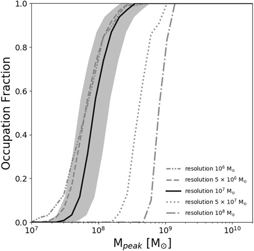
Impact of resolution on the predicted occupation fraction as a function of the peak halo mass. Line types depict different resolutions, with the grey double-dotted–dashed, dashed, dotted, and dashed–dotted lines corresponding to resolutions of 106, 5 × 10⁶, 5 × 10⁷, and 108 M⊙, respectively. The black solid line represents our fiducial 107M⊙ resolution, along with the uncertainty of the peak mass measurements from our results, which is depicted by the grey-shaded region.
We also examined the influence of resolution on the predicted metallicity of the satellites. As depicted in Fig. D2, at higher stellar masses for the subhaloes, we did not observe substantial differences resulting from resolution changes. However, at the lower mass range, altering the resolution introduced some variations in the metallicity predictions. These discrepancies could be attributed to the effects of bias in selecting the low stellar mass population due to the sharp resolution-induced cut-off in the SMHM relation within our results. In such cases, lower resolution would lead to a subhalo population with biased higher stellar masses (due to the resolution cut-off), which can statistically shift the median metallicity towards larger values. Additionally, we excluded the IGM metallicity from our model and compared its impact. The results demonstrated a similar behaviour with slightly reduced significance.
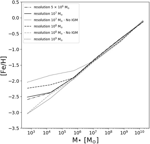
Effect of resolution on the mass–metallicity relation. The mass–metallicity relation is shown with various black line styles representing different resolutions. Resolution 107M⊙ is represented by the solid black line, while resolutions 5 × 10⁶, 108, and 109 M⊙ are depicted by the dotted–dashed, dashed, and dotted black lines, respectively. Additionally, the corresponding models without the inclusion of IGM metallicity are shown with grey lines, with solid and dotted lines representing resolutions 107 and 108 M⊙, respectively.
