


ABSTRACT
Detailed chemical studies of F/G/K – or solar-type – stars have long been routine in stellar astrophysics, enabling studies in both Galactic chemodynamics and exoplanet demographics. However, similar understanding of the chemistry of M and late-K dwarfs – the most common stars in the Galaxy – has been greatly hampered both observationally and theoretically by the complex molecular chemistry of their atmospheres. Here, we present a new implementation of the data-driven Cannon model, modelling Teff, log g, [Fe/H], and [Ti/Fe] trained on low–medium resolution optical spectra (4000–7000 Å) from 103 cool dwarf benchmarks. Alongside this, we also investigate the sensitivity of optical wavelengths to various atomic and molecular species using both data-driven and theoretical means via a custom grid of MARCS synthetic spectra, and make recommendations for where MARCS struggles to reproduce cool dwarf fluxes. Under leave-one-out cross-validation, our Cannon model is capable of recovering Teff, log g, [Fe/H], and [Ti/Fe] with precisions of 1.4 per cent, |$\pm 0.04\,$| dex, |$\pm 0.10\,$| dex, and |$\pm 0.06\,$| dex respectively, with the recovery of [Ti/Fe] pointing to the as-yet mostly untapped potential of exploiting the abundant – but complex – chemical information within optical spectra of cool stars.
1 INTRODUCTION
The solar neighbourhood – and indeed the Universe more broadly – is dominated by cool dwarf stars of spectral types K and M (e.g. Henry, Kirkpatrick & Simons 1994; Chabrier 2003; Henry et al. 2006; Winters et al. 2015; Henry et al. 2018). While Milky Way stars in general are expected to host at least one planet on average (Cassan et al. 2012), cool dwarfs are actually more likely to host small planets as compared to more massive stars (Howard et al. 2012; Dressing & Charbonneau 2015) with many yet undiscovered (Morton & Swift 2014). Enabled by the space-based Kepler (Borucki et al. 2010), K2 (Howell et al. 2014), and TESS (Ricker et al. 2015) missions, exoplanetary astrophysics now has a large and ever-growing set of such systems to study both individually in detail, as well as collectively in a demographic sense.
When presented as such, it is easy to come to the conclusion that cool dwarfs and their planets are as well-understood as their prevalence might imply. In reality though, these stars are intrinsically faint – especially at optical wavelengths – and possess complex spectra blanketed by innumerable overlapping molecular absorption features. In the infrared (IR), this absorption is dominated by molecules like H2O, CO, FeH, and OH; and in the optical from oxides like TiO, ZrO, and VO, as well as hydrides like MgH, CaH, AlH, and SiH. Such complexity renders the spectral energy distribution not just a strong function of temperature, as with solar-type stars, but also chemistry, making it difficult to ascribe an accurate or unique set of stellar parameters to any given star. This intense molecular absorption makes ‘true’ continuum normalization impossible at optical wavelengths, and poses severe challenges for traditional spectroscopic analysis techniques. As a result, our understanding of the chemistry of cool dwarfs and their planets typically lags far behind those of solar-type stars.
This atmospheric complexity and the large impact a single molecular species can have on an emergent spectrum means that the generation of model spectra that accurately match observations has been, and continues to be, a challenge. While model spectra at cool temperatures demonstrate reasonable performance in the near infrared (NIR; e.g. Allard et al. 1997; Baraffe et al. 1997, 1998; Allard, Homeier & Freytag 2012), there have long been issues in the optical (e.g. Baraffe et al. 1998; Reylé et al. 2011; Mann, Gaidos & Ansdell 2013c; Rains et al. 2021). The core reason is likely incomplete line lists for dominant sources of opacity, where the impact of not accurately knowing transition wavelengths or line depths can be severe (e.g. Plez, Brett & Nordlund 1992; Masseron et al. 2014) – particularly for TiO (e.g. Hoeijmakers et al. 2015; McKemmish et al. 2019) which dominates absorption in the optical. All this means that, to this day, it is far from simple to produce accurate cool dwarf temperatures, radii, and especially metallicities en masse – let alone individual elemental abundances.
Given these complexities, it is thus critical to have a set of cool dwarfs of known chemistry to use as benchmarks for testing models or building empirical relations. The widely considered gold standard are cool dwarfs in binary systems with a warmer companion of spectral type F/G/K from which the chemistry can more easily be determined. This relies on the assumption that both stars formed at the same time and thus have the same chemical composition. Thankfully such chemical homogeneity is now well established for F/G/K–F/G/K pairs (e.g. Desidera et al. 2004; Simpson et al. 2019; Hawkins et al. 2020; Yong et al. 2023), and while there remain edge-cases of chemically inhomogeneous pairs (e.g. Spina et al. 2021) – possibly the result of planet engulfment – the level of chemical homogeneity is more than sufficient for the precision of the current state of the art in cool dwarf chemical analysis.
The extreme sensitivity of cool dwarf spectra to stellar chemistry remains present in broad-band optical photometry, though this is less the case in the IR where K-band photometry at |$2.2\, \mu$|m is a comparatively [Fe/H]–insensitive1 probe of stellar mass (M⋆) for isolated main-sequence stars with |$M_\star \lesssim 0.7\, {\rm M}_\odot$|. This is something that was initially predicted by theory (see e.g. Allard et al. 1997, Baraffe et al. 1998, and Chabrier & Baraffe 2000 for summaries), and later confirmed observationally (Delfosse et al. 2000), and allows for the development of photometric metallicity relations using an optical–NIR colour benchmarked on the aforementioned K/M–F/G/K benchmark systems (e.g. Bonfils et al. 2005; Johnson & Apps 2009; Schlaufman & Laughlin 2010; Neves et al. 2012; Hejazi, De Robertis & Dawson 2015; Dittmann et al. 2016; Rains et al. 2021; Duque-Arribas et al. 2023). While purely photometric metallicity relations suffer from certain limitations, such as their sensitivity to unresolved binarity or young stars still contracting to the main sequence – they are widely applicable given the volume of data available from photometric surveys like 2MASS (Skrutskie et al. 2006), SkyMapper (Keller et al. 2007), SDSS (York et al. 2000), Pan-STARRS (Chambers et al. 2016), and Gaia (Gaia Collaboration 2016).
Greater metallicity precision can be achieved by using low-resolution spectra and building empirical relations from [Fe/H]-sensitive spectral regions or indices, again benchmarked against K/M–F/G/K binary systems. Such low-resolution spectra contain vastly more information than broad-band photometry alone and are relatively observationally cheap to obtain, especially at redder wavelengths (e.g. the YJHK bands) where these stars are brighter. The last ∼10 yr has seen a number of studies develop such relations, which span a range of spectral resolutions and wavelengths (e.g. Rojas-Ayala et al. 2010, 2012; Terrien et al. 2012; Mann et al. 2013b; Mann, et al. 2013c; Newton et al. 2014; Mann et al. 2015; Kuznetsov et al. 2019), which importantly gives rise to a large secondary set of fundamentally calibrated cool dwarf benchmarks. This proves useful as the wide separation F/G/K–M/K binaries passing the quality cuts necessary to serve as benchmark systems are more rare – and thus also more distant on average – making the secondary set of benchmarks the brighter and more populous sample.
Other studies have opted to determine [Fe/H] from model fits to high-resolution spectra. Not only can this give access to unblended atomic lines not accessible for observations made at lower spectral resolution – especially in the (N)IR – but it also allows for more detailed testing of the models themselves.2 These studies span a similarly wide range of optical and IR wavelengths (e.g. Woolf & Wallerstein 2005, 2006; Bean et al. 2006a; Bean, Benedict & Endl 2006b; Rajpurohit et al. 2014; Passegger, Wende-von Berg & Reiners 2016; Lindgren & Heiter 2017; Souto et al. 2017; Veyette et al. 2017; Passegger et al. 2018; Marfil et al. 2021; Cristofari et al. 2022a), and have helped in pushing the boundaries of what we know about cool dwarfs and how best to model and analyse them.
However, despite these advances in the determination of cool dwarf metallicities, it is at best an approximation to assume that their spectra can reliably be parametrized by only three atmospheric parameters in Teff, log g, and [M/H] (or [Fe/H], its common proxy3). In reality, individual elemental abundances are able to dramatically change the shape of the observed ‘pseudo-continuum’ – and thus the measured stellar properties – via their effect on various dominant molecular absorbers. As a specific example, Veyette et al. (2016) demonstrated that independently changing carbon and oxygen abundances by just |$\pm 0.2\,$|dex can result in an inferred metallicity ranging over a full order of magnitude (|$\gt 1\,$| dex), with typical metallicity indicators – like those from low-resolution spectra previously discussed – showing a strong dependence on the C/O ratio. In cool atmospheres the carbon abundance affects how much oxygen gets locked up in CO, a low-energy molecule that preferentially forms, with only the leftover oxygen able to go into other dominant opacity sources like H2O and TiO.
Understanding elemental abundances of cool dwarfs beyond just the bulk metallicity is thus a critically important task. This important work is well underway (e.g. Tsuji & Nakajima 2014; Tsuji, Nakajima & Takeda 2015; Tsuji 2016; Tsuji & Nakajima 2016; Veyette et al. 2016; Souto et al. 2017; Veyette et al. 2017; Souto et al. 2018; Ishikawa et al. 2020; Maldonado et al. 2020; Souto et al. 2020; Ishikawa et al. 2022; Souto et al. 2022; Cristofari et al. 2022b), but more research is needed to fundamentally calibrate the results using a larger set of more chemically diverse binary benchmarks, do this at the scale of large spectroscopic surveys containing thousands of stars, and to use this knowledge to improve upon the current generation of cool dwarf model spectra.
Data-driven models present another method to tackling this problem. Provided they are trained on spectra from a set of benchmarks with precise fundamental or fundamentally-calibrated properties, such an approach becomes an effective way of teasing apart the complex chemistry of these stars. Absent the limitations that come with physical models (e.g. incomplete molecular line lists), data-driven models have the potential to turn what is traditionally considered a weakness of cool dwarfs – strong and innumerable overlapping absorption features from multiple different atomic and molecular species – into a strength given the sheer amount of information present – assuming of course this chemical information can be properly exploited. This is a particularly important problem to solve in preparation for upcoming massive spectroscopic surveys like 4MOST (de Jong et al. 2019) and SDSS-V (Kollmeier et al. 2017).
Data-driven models like the Cannon (Ness et al. 2015) have been successfully applied to F/G/K stars observed by spectroscopic surveys like GALAH, APOGEE, LAMOST, and SPOCS (e.g. Casey et al. 2016; Ho et al. 2016; Buder et al. 2018; Casey et al. 2019; Rice & Brewer 2020; Wheeler et al. 2020; Nandakumar et al. 2022), often with the goal of inter-survey comparison or the computational speed of data-driven stellar property determination versus more traditional modelling. Other studies have extended this work to cool (and brown) dwarfs using a variety of modelling approaches (Behmard, Petigura & Howard 2019; Birky et al. 2020; Galgano, Stassun & Rojas-Ayala 2020; Li et al. 2021; Feeser & Best 2022) for the recovery of properties like spectral type, Teff, log g, [Fe/H], [M/H], M⋆, stellar radius (R⋆), or stellar luminosity (L⋆), with Maldonado et al. (2020) even reporting the impressive recovery of 14 different chemical abundances with |$\Delta {\rm [X/H]}\lesssim 0.10\,$| dex for their sample of K/M–F/G/K binaries. Finally, these models can also be used to explore complex parameter spaces and make new physical insights – for example wavelength regions sensitive to particular elemental abundances – something more challenging to do with traditional analysis methods.
Here, we present a new implementation of the Cannon trained on low-to-medium resolution (R ∼ 3000–7000) optical spectra (|$4000 \lt \lambda \lt 7000\,$| Å) of cool dwarfs observed with the WiFeS instrument (Dopita et al. 2007) on the ANU 2.3 m Telescope at Siding Spring Observatory (NSW, Australia). Our four label model in Teff, log g, [Fe/H], and [Ti/Fe] draws its accuracy from a relatively small, but hand-selected, set of 103 stellar benchmarks primarily composed of stars with interferometric Teff, [Fe/H] and [Ti/Fe] measurements from a wide binary companion of spectral type F/G/K, or [Fe/H] determined from binary-benchmarked empirical relations based on low-resolution NIR spectra. We use our Cannon model in conjunction with a custom grid of MARCS model spectra (Gustafsson et al. 2008) to investigate the sensitivity of optical cool dwarf fluxes to variations in chemical abundances, as well as limitations in reproducing optical fluxes. Our data and stellar benchmark selection are described in Section 2; our Cannon model and its training, validation, and performance in Section 3; an investigation into cool dwarf optical flux sensitivity to elemental abundance variations using MARCS spectra in Section 4; a discussion of results, comparison to previous work, MARCS flux recovery assessment, and future prospects in Section 5; and concluding remarks in Section 6.
2 COOL DWARF BENCHMARK SAMPLE
2.1 Spectroscopic data
Our data consists of low- and medium-resolution optical benchmark stellar spectra observed with the dual-camera WiFeS instrument (Dopita et al. 2007) on the ANU 2.3 m Telescope as part of the spectroscopic surveys published as Žerjal et al. (2021) and Rains et al. (2021). All stars were observed with the B3000 and R7000 gratings using the RT480 beam splitter, yielding low-resolution blue spectra (|$3500 \le \lambda \le 5700\,$| Å, λ/Δλ ∼ 3000) and moderate resolution red spectra (|$5400 \le \lambda \le 7000\,$| Å, λ/Δλ ∼ 7000). This benchmark sample is described in Section 2.2, and is plotted as a colour–magnitude diagram in Fig. 1.
![2MASS$M_{K_S}$ versus Gaia DR3 (BP − RP) colour magnitude diagram for our 103 selected cool dwarf benchmarks, coloured according to their adopted [Fe/H]. The subsample of benchmarks with chemistry from an F/G/K binary companion are outlined.](https://oup.silverchair-cdn.com/oup/backfile/Content_public/Journal/mnras/529/4/10.1093_mnras_stae560/1/m_stae560fig1.jpeg?Expires=1749174622&Signature=uhbp0KDaDgRLDMmRXHn-6XFFis0boWVva6X6hPFrbHTBiTDwKqt4F65G452~2h4Gj99jch~1I7429uKUkdM~ZsfkA-QpiBnr5gHcFrSA39Z9MBtKASDrfIDGCMKSUUBcI9dYYUW6AMgjMbdKxgSD2h~0IO3yIRBR0KTGYADuUgpSOvLPPF8vSXzQ1pxI20p-WVW2CvsApCv-nlI8ZG-icIxikWodLw-3~CnrAnYp8v3DYW4swFP-P-QlHQ3yCko69sC9vxCcdZN-uGuwcDgJC1Jtxr6JH1RDtOr~rOsnyYfp8SlO8SqCC3MwV1VLKqmofdIxgF0ZeYUxnZKS0x8nBA__&Key-Pair-Id=APKAIE5G5CRDK6RD3PGA)
2MASS|$M_{K_S}$| versus Gaia DR3 (BP − RP) colour magnitude diagram for our 103 selected cool dwarf benchmarks, coloured according to their adopted [Fe/H]. The subsample of benchmarks with chemistry from an F/G/K binary companion are outlined.
Our spectra were reduced using the standard PyWiFeS pipeline (Childress et al. 2014) using the flux calibration approach of Rains et al. (2021), but remain uncorrected for telluric absorption which we treat by simply masking the worst-affected wavelength regions. Radial velocities were determined by fitting against a template grid of MARCS synthetic spectra as described in Žerjal et al. (2021), and our spectra were subsequently shifted to the rest frame via linear interpolation using the interp1d function from scipy’s interpolate module in python.4
2.2 Benchmark stellar parameters
To train a data-driven model, we require a set of stellar parameters to train on. Like previous studies, we adopt the three ‘core’ stellar parameters of Teff, log g, and [Fe/H], but distinguish ourselves by studying an additional chemical dimension in [Ti/Fe]. The primary motivation for selecting [Ti/Fe] as our abundance of choice to investigate is due to the strong expected signature of TiO on our optical spectra, something we expect to correlate with [Ti/Fe].5 Though we also expect strong optical signatures from C and O per Veyette et al. (2016), these elements have fewer absorption lines in the optical than Ti, and thus literature abundances sources from high-resolution spectroscopy are less prevalent. Finally, while we expect strong signatures from other oxides and hydrides on our spectra, we limit ourselves to two chemical dimensions in [Fe/H] and [Ti/Fe] for the purposes of this initial study with our relatively small sample size.
When selecting our benchmark sample of cool dwarfs, our objective was to use only those stars with fundamental – or fundamentally calibrated – stellar parameters.6 A large factor motivating our decision to pursue a data-driven approach stems from the incomplete and physically inaccurate nature of current generation synthetic optical spectra used in more traditional analyses. Given our goal is to avoid, or even shed light on these limitations, and the accuracy of a data-driven model is only as good as its training sample, we must then be very selective.
Thus, our benchmark sample is composed of 103 cool dwarfs with stellar parameters from at least one of the following categories:7
[Fe/H] or [Ti/Fe] from an F/G/K companion,
[Fe/H] from empirical relations based on low resolution NIR spectra and calibrated to (i),
Teff from interferometry,
where 17 stars have [Fe/H] and [Ti/Fe] from a warmer binary companion, 93 have [Fe/H] from NIR empirical relations, and 17 stars have interferometric Teff. For those stars not in binary systems, we determine [Ti/Fe] based on chemodynamic trends present in Gaia DR3 (Vallenari et al. 2023) and GALAH DR3 (Buder et al. 2021) data. While small, we note that such a limited training sample has precedent in studies like Behmard et al. (2019), Birky et al. (2020), and Maldonado et al. (2020).
In addition to these parameter-specific requirements, we also impose two additional quality constraints on our sample. First, to ensure we have a clean sample free from obvious unresolved binaries, we require benchmarks have a Gaia DR3 Renormalized Unit Weight Error (RUWE) of <1.4, above which the single star astrometric fit is deemed poor by the Gaia Consortium (e.g. Belokurov et al. 2020; Lindegren et al. 2021). Secondly, we reject binary benchmarks with inconsistent Gaia DR3 kinematics between the primary and secondary components in order to better guarantee our gold standard chemical benchmarks are physically associated.
The following sections describe our literature sources for each separate stellar parameter, as well as our adopted hierarchy between sources for those stars with more than a single source: Section 2.2.1: Teff, Section 2.2.2: log g, Section 2.2.3: [Fe/H], Section 2.2.4: [Ti/Fe] from binaries, and Section 2.2.5 [Ti/Fe] from empirical chemodynamic trends. Table 1 serves as a summary of these subsections, with sources listed in order of preference when choosing which to adopt (included inter-sample systematics where measured).
Summary of literature Teff, log g, [Fe/H], and [Ti/Fe] sources referenced for our stellar benchmark sample, ordered from highest to lowest preference of label adoption. We list the median label uncertainty of each source and for our adopted set of labels as a whole, any intersample label systematics, benchmark stars with labels from each sample, benchmark stars without labels from each sample, and benchmark stars whose labels we adopt from each sample. We use Valenti & Fischer (2005) as our reference for computing [Fe/H] and [Ti/Fe] offsets that accounts for both reference abundance scale differences and other related systematics.
| Label | Sample | Median σlabel | Offset | Nwith | Nwithout | Nadopted |
|---|---|---|---|---|---|---|
| Teff | All | 67 K | – | 103 | 0 | 103 |
| Interferometry | 25 K | – | 17 | 86 | 17 | |
| Rains+21 | 67 K | – | 103 | 0 | 86 | |
| log g | All | 0.02 dex | – | 103 | 0 | 103 |
| Rains+21 | 0.02 dex | – | 103 | 0 | 103 | |
| [Fe/H] | All | 0.08 dex | – | 103 | 0 | 103 |
| Brewer+2016 | 0.01 dex | +0.00 dex | 7 | 96 | 7 | |
| Rice & Brewer (2020) | 0.01 dex | +0.00 dex | 4 | 99 | 4 | |
| Valenti & Fischer (2005) | 0.03 dex | +0.00 dex | 10 | 93 | 1 | |
| Montes+2018 | 0.04 dex | +0.02 dex | 15 | 88 | 4 | |
| Sousa+2008 | 0.03 dex | – | – | – | 1 | |
| Mann+2015 | 0.08 dex | +0.00 dex | 75 | 28 | 69 | |
| Rojas-Ayala+2012 | 0.12 dex | +0.01 dex | 33 | 70 | 12 | |
| Other NIR | 0.08 dex | – | – | – | 3 | |
| Photometric | 0.19 dex | – | 98 | 5 | 2 | |
| [Ti/Fe] | All | 0.04 dex | – | 103 | 0 | 103 |
| Brewer+2016 | 0.02 dex | −0.02 dex | 7 | 96 | 7 | |
| Rice & Brewer 2020 | 0.04 dex | +0.00 dex | 4 | 99 | 4 | |
| Valenti & Fischer 2005 | 0.05 dex | +0.00 dex | 10 | 93 | 1 | |
| Montes+2018 | 0.07 dex | −0.03 dex | 15 | 88 | 4 | |
| Adibekyan+2012 | 0.06 dex | – | – | – | 1 | |
| This Work | 0.07 dex | −0.03 dex | 103 | 0 | 86 |
2.2.1 Stellar Teff
Interferometric temperature benchmarks form the cornerstone of our data-driven temperature scale, and thus we observed 17 stars from van Belle & von Braun (2009), Boyajian et al. (2012), von Braun et al. (2012), von Braun et al. (2014), and Rabus et al. (2019) with a median literature Teff uncertainty of |$\pm 25\,$| K. This left a decision on what temperatures to adopt for the remainder of our benchmark sample, specifically with how we handle systematics between different temperature scales or those stars without a previously reported value (mainly our binary benchmarks). As an example, the bulk of our NIR [Fe/H] benchmarks have Teff from either Rojas-Ayala et al. (2012) or Mann et al. (2015), with Mann et al. (2015) noting temperature systematics between the overlapping samples between the two studies at warmer Teff.8 Given this concern, we deemed the use of a single uniform Teff scale for our benchmark sample critical in order to have the best chance of investigating cool dwarf chemistry. To this end, for all non-interferometric benchmarks we adopt Teff obtained via the fitting methodology of Rains et al. (2021) – itself calibrated to our adopted interferometric scale. We describe this method below, and add our statistical uncertainties in quadrature with the median benchmark Teff uncertainty for a final median uncertainty of |$\pm 67\,$|K.
Rains et al. (2021) undertook a benchmark-calibrated joint synthetic fit to spectroscopic and photometric data using flux calibrated WiFeS spectra and literature Gaia/2MASS/SkyMapper photometry for their cool dwarf sample. As a necessity for model-based work with cool optical fluxes, they quantified model systematics by comparing synthetic MARCS spectra and photometry to observed spectra and integrated photometry from their benchmark sample of 136 cool dwarf benchmarks with |$3,000 \lesssim T_{\rm eff} \lesssim 4,500\,$| K. These systematics, parametrized as a function of Gaia (BP − RP) colour, were used to correct synthetic photometry during fitting, with only the most reliable regions in the WiFeS R7000 spectral arm being included. Teff was the principal output of their fit, with both log g and [Fe/H] fixed using empirical relations (the former from Mann et al. 2015 and Mann et al. 2019, the latter developed in Rains et al. 2021) to avoid parameter degeneracies due to the complexity of cool dwarf fluxes. Reported temperatures were calibrated to a fundamental scale by correcting for temperature systematics observed between fits to the aforementioned benchmark sample, itself fundamentally calibrated to the interferometric Teff scale.
2.2.2 Stellar log g
For stellar log g, we also adopt the uniform values from Rains et al. (2021). Due to model limitations and degeneracies, Rains et al. (2021) fixed log g when fitting for Teff and used a two-step iterative process to determine the final gravity. Initial M⋆ and R⋆ values were obtained from the photometric |$M_{K_S}$| band relations in Mann et al. (2019) and Mann et al. (2015), respectively, and were used to compute and fix log g for the initial fit. Following this initial fit, R⋆ was recalculated from the fitted Teff and fbol values via the Stefan Boltzmann relation, log g recalculated, and a final fit performed to give the adopted stellar R⋆ and log g. It should be noted, however, that this process is almost entirely based on photometry, meaning that we are not sensitive to unresolved binarity or youth in the same way that spectroscopic techniques are. The median log g statistical uncertainty of our benchmark sample is |$\pm 0.02\,$| dex.
2.2.3 Stellar [Fe/H]
The inability to recover [Fe/H] from optical cool dwarf spectra makes the selection of [Fe/H] benchmarks particularly crucial for any data-driven approach. The gold standard for cool dwarf metallicities continues to be those stars with a warmer companion of spectral type F/G/K from which traditional spectral analysis techniques like measuring equivalent widths or spectral synthesis are reliable. We adopt [Fe/H] from these stars where possible, sourced from Valenti & Fischer (2005), Sousa et al. (2008), Brewer et al. (2016), Montes et al. (2018), and Rice & Brewer (2020). These are our most precise [Fe/H] benchmarks, with −0.86 < [Fe/H] < 0.35,9 with a median literature uncertainty of |$\pm 0.03\,$| dex for the 17 such stars in our sample.
We adopt Valenti & Fischer (2005) as our reference when computing and correcting for [Fe/H] and [Ti/H] systematics (see the ‘offset’ column in Table 1), though prioritise Brewer et al. (2016) and Rice & Brewer (2020) – both follow-up studies – for their higher precision. Valenti & Fischer (2005) was chosen as our reference scale due to its large sample size and the fact that Mann et al. (2013a) – the original source for the [Fe/H] relations used in Mann et al. (2015) – also used it as their [Fe/H] reference point. Note that different sources in Table 1 adopt different abundance reference points, either published reference abundance levels or their own solar-relative abundances, and this results in straightforward differences in [Fe/H] scales. However, there exists the possibility for other effective systematics present due to e.g. differences in the temperature scale, and these will not be apparent from a simple comparison between abundance scales – but are accounted for by our approach of identifying and removing systematics between samples. Finally, when computing offsets we do so using a larger cross-matched set of literature F/G/K–K/M binary benchmarks than we have spectra for here, with 256 primaries and 259 secondaries in total (noting that not all of these stars are in all publications).
Our largest sample of [Fe/H] comes from empirical relations built from [Fe/H] sensitive spectral regions in low-resolution NIR spectra based on these binary benchmarks. While there are many such relations in the literature, the bulk of our stars are drawn from just two of them. 69 of our stars have [Fe/H] from the work of Mann et al. (2015), with |$\sigma _{\rm [Fe/H]}=\pm 0.08\,$| dex. Another 12 are drawn from the work of Rojas-Ayala et al. (2012), with |$\sigma _{\rm [Fe/H]}=\pm 0.18\,$| dex. Only three stars have adopted [Fe/H] from other relations, with one star from Terrien et al. (2015) with |$\sigma _{\rm [Fe/H]}=\pm 0.07\,$| dex, and another two from Gaidos et al. (2014) with |$\sigma _{\rm [Fe/H]}=\pm 0.1\,$| dex.
Finally, for any star without [Fe/H], we adopt [Fe/H] from the photometric relation of Rains et al. (2021) with |$\sigma _{\rm [Fe/H]}=\pm 0.19\,$| dex. This relation is only applicable to isolated single stars on the main sequence with reliable Gaia parallaxes. In our case, only two stars – GJ 674 and GJ 832, both interferometric benchmarks – have a value from this relation. However, this ensures that all stars in our sample have an [Fe/H] value.
2.2.4 Measured stellar [Ti/Fe]
For those benchmark stars in F/G/K–K/M binary systems, we can adopt [Ti/Fe] abundances from the warmer primary where they it has previously been measured in the literature. Per Table 1, we adopt [Ti/Fe] for seven stars from Brewer et al. (2016), four stars from Rice & Brewer (2020), one star from Valenti & Fischer (2005), four stars from Montes et al. (2018), and one star from Adibekyan et al. (2012). We note that Brewer et al. (2016) and Rice & Brewer (2020) are follow-up work to Valenti & Fischer (2005), and thus we preference them due to their higher [Ti/H] precision (while again adopting Valenti & Fischer 2005 as our adopted reference for [Ti/H] systematics), and for Adibekyan et al. (2012) we adopt the abundance derived from Ti i lines. Each of these works report abundances as [X/H], so we have calculated [Ti/Fe] using the adopted systematic-corrected [Fe/H] values (typically from the same literature source) and propagated the uncertainties accordingly, resulting in a median uncertainty of |$\sigma _{\rm [Ti/Fe]}=\pm 0.03\,$| dex.
2.2.5 Empirical chemodynamic [Ti/Fe]
To assign [Ti/Fe] values for non-binary benchmarks, we make use of chemodynamic correlations in the Milky Way (MW) discs to ‘map’ [Ti/Fe] values onto the benchmark stars. The chemical distinctness of the thick and thin discs in light elements (e.g. Mg, Ca, O, Si, Ti, or the α-elements) across metallicities has become a well-accepted feature of our galaxy (e.g. as observed early-on in high resolution studies of small samples and in the larger APOGEE survey, Nissen & Schuster 2010; Hayden et al. 2015). To map values of [Ti/Fe], we utilize the GALAH DR3 data release (Buder et al. 2021) to recover chemistry and the value added catalogue (VAC) of Buder et al. (2022) for the stellar kinematics. Initial estimates of component membership (e.g. thick or thin disc) were made by comparing the energy (E) and z-component of the angular momentum (Lz) of the benchmark stars to a subset of the GALAH DR3 sample. The GALAH subset was selected to only include dwarf stars with similar stellar parameters to the F/G/K primaries of our binary benchmark stars (Teff > 4500 K and log g > 3.0) and to exclude stars with potentially unreliable chemistry (i.e. cool stars). The E, Lz values for the benchmarks were recovered assuming the McMillan2017 (McMillan 2017) approximation for the MW potential and assuming a solar radius of 8.21 kpc and a circular velocity at the Sun of 233.1 km s−1. The local standard of rest (LSR) was selected to be in the same frame of reference as the GALAH VAC. That is, the Sun is set 25 pc above the plane in keeping with Jurić et al. (2008) and has a total velocity of (U, V, W) = (11.1, 248.27, 7.25) km s−1 in keeping with Schönrich, Binney & Dehnen (2010).
Unsurprisingly, all of the benchmark stars are found to be on nearly circular orbits, coincident with either the MW thick or thin disc in E, Lz space. In addition to calculating the E, Lz values for the benchmarks, we also calculated the vϕ values for the stars (the tangential velocity component in cylindrical coordinates) under the same assumption and orientation of the LSR. Following an exploration of various chemodynamic spaces, we found vϕ versus [Fe/H] to isolate the [α/Fe] bimodality (associated with the thick and thin discs, Nissen & Schuster 2010) the most cleanly. This is shown for a subset of GALAH stars in the left panel of Fig. 2 where we have removed the bulk of the stellar halo by applying the cut, vϕ > 100 km s−1. The clean GALAH disc sample is binned into 100 bins in vϕ, [Fe/H] and coloured by the average value of [Ti/Fe] in each bin. The benchmark stars are overplotted in the right-hand panel of Fig. 2 to highlight their association with the thick (high [Ti/Fe], low vϕ) and thin (low [Ti/Fe], high vϕ) discs.
![Left: The ‘mapped’ values of [Ti/Fe] for the benchmarks (black circles) using their vϕ, [Fe/H] values, and interpolation of the space presented in the right panel. The average values are calculated following 1000 draws sampling the errors associated with [Fe/H] and the input astrometric parameters from Gaia DR3. The GALAH disc sample is plotted underneath. Right: The distribution of a subset of GALAH DR3 stars with large vϕ ($\gt 100\,$ km s−1) selected to isolate the thick and thin MW discs. The subset is binned and coloured by the average [Ti/Fe] value of the bin (note the recovery of the [α/Fe] bimodality). Benchmark stars are overplotted as open circles, where their vϕ values have been calculated under the LSR discussed in Section 2.2.5.](https://oup.silverchair-cdn.com/oup/backfile/Content_public/Journal/mnras/529/4/10.1093_mnras_stae560/1/m_stae560fig2.jpeg?Expires=1749174622&Signature=YLwx2D30Xucw4~IUupLZA990W0XmBeEZGUH5h5wPYtmqNMQv2wKbUQDeVg-LGE-QyoLhU68XBMSU5qHqIkdFdfxe5wf9pQ~GX3lcm1K4t237kR1iM8U3sGxOdlOKnrjeYOLsj5ngBcMjPtTtiyQJz94hn74VYaoFPaA8JnDSx~qsTu~B9fZNQOyHhPynDc2Zt5IFW~Rb-B1ab9XTOQnjhvZwaL8BGCQ9hDLfS-8vOCTrX5~ND4r3McdCHPJrzanc-6vAM7sd59PwoZuEue1KcCN0S9DrFFU-9OJtgQ516LEopK739hs~vDiZT4SVfOfd-K8hDeG5j2JXg5xspjNlrQ__&Key-Pair-Id=APKAIE5G5CRDK6RD3PGA)
Left: The ‘mapped’ values of [Ti/Fe] for the benchmarks (black circles) using their vϕ, [Fe/H] values, and interpolation of the space presented in the right panel. The average values are calculated following 1000 draws sampling the errors associated with [Fe/H] and the input astrometric parameters from Gaia DR3. The GALAH disc sample is plotted underneath. Right: The distribution of a subset of GALAH DR3 stars with large vϕ (|$\gt 100\,$| km s−1) selected to isolate the thick and thin MW discs. The subset is binned and coloured by the average [Ti/Fe] value of the bin (note the recovery of the [α/Fe] bimodality). Benchmark stars are overplotted as open circles, where their vϕ values have been calculated under the LSR discussed in Section 2.2.5.
To map a value of [Ti/Fe] to the benchmark stars, we performed a 2D interpolation of the clean GALAH disc sample in vϕ, [Fe/H] space using the N-dimensional linear interpolator in scipy (Virtanen et al. 2020). To explore the uncertainty associated with the benchmark chemodynamics, we perform 1000 realizations sampling normal distributions in [Fe/H], and radial velocity (RV) and the multivariate distribution associated with the uncertainties in the astrometric parameters. We build the astrometric covariance matrix using the correlations and errors for the benchmarks within Gaia DR3 (Lindegren et al. 2021). The vϕ values are then recalculated for each draw and the corresponding vϕ, [Fe/H] values are used to infer a [Ti/Fe] for the star. The average recovered values of [Ti/Fe] for the benchmarks are shown in the left panel of Fig. 2 as the open circles. They are overplotted on-top of the clean GALAH disc sample (shown as the black points). Note that the uncertainties are largest for the lowest metallicity benchmarks. This is likely a result of the metallicity distribution function of the thick disc being less well-sampled in our GALAH subset. This in itself it likely driven by our conservative cut in vϕ to remove the bulk of the MW halo (which presents a much more complex trend of light elements with metallicity).
To both validate our methodology and place GALAH and our benchmark stars on the same scale, we repeated the same exercise to predict [Ti/Fe] on the sample of dwarf stars from Valenti & Fischer (2005). Fig. 3 shows the comparison between our predicted values of [Ti/Fe] and those published in Valenti & Fischer (2005) for stars with |$\mathrm{[Fe/H]}\ge -1\,$| dex. When considering the 1 019 stars that meet our requirement in [Fe/H], we recover a median offset between the predicted and true values of [Ti/Fe] of |$0.03\,$|dex, with the residuals having a standard deviation of |$0.08\,$| dex. We correct for this offset in order to anchor our predicted [Ti/Fe] values to the Valenti & Fischer (2005) scale, and take the uncertainty of our mapping to be |$\sigma _{\rm [Ti/Fe]}=0.08\,$| dex per the standard deviation.
![Literature [Ti/Fe] abundance for 1 029 stars from Valenti & Fischer (2005) versus [Ti/Fe] as predicted from Gaia and GALAH chemodynamic trends as in Section 2.2.5, with the median and standard deviation of the residuals annotated. The black circled points correspond to the F/G/K primaries of our binary benchmarks. Note that we correct for the observed [Ti/Fe] systematic – that is we put our GALAH [Ti/Fe] values on the Valenti & Fischer (2005) scale – and that the observed value of σ[Ti/Fe] is comparable with the mapped [Ti/Fe] statistical uncertainties for our sample quoted in Table 1 when taking into account [Fe/H] and kinematic uncertainties.](https://oup.silverchair-cdn.com/oup/backfile/Content_public/Journal/mnras/529/4/10.1093_mnras_stae560/1/m_stae560fig3.jpeg?Expires=1749174622&Signature=TZvZfzzpZ0DZyMoTvQVHL39DPN2Mf2fATRgOylEPxarAO-3D4oSFXa~fIP2T1Rvk2yIr3Sxk-SXPdCUr02UshaLHx5C7-Wp4QkIEn-F-OaCHdigcmpPhnfK215NyUn8q15vqxLC82sqCmQVIDD5jbJcB1gpCyhpy0qoSCUxTQg8QZK2JFMiJEcQmHST9pCoCIwGrz9YPxV870mVt3bpA502aBEWMqkYWIwF9d2vufa22dlDFzBFNeQcweQI7XS1SNxvW2OJ5UP6ew7Ei~qcg-OsNXwWWqLxDGkijM21M08pAt5lKPkkpJT3wrp52QbxWb1xnVZX9PTCbvbKh9ZdI7Q__&Key-Pair-Id=APKAIE5G5CRDK6RD3PGA)
Literature [Ti/Fe] abundance for 1 029 stars from Valenti & Fischer (2005) versus [Ti/Fe] as predicted from Gaia and GALAH chemodynamic trends as in Section 2.2.5, with the median and standard deviation of the residuals annotated. The black circled points correspond to the F/G/K primaries of our binary benchmarks. Note that we correct for the observed [Ti/Fe] systematic – that is we put our GALAH [Ti/Fe] values on the Valenti & Fischer (2005) scale – and that the observed value of σ[Ti/Fe] is comparable with the mapped [Ti/Fe] statistical uncertainties for our sample quoted in Table 1 when taking into account [Fe/H] and kinematic uncertainties.
3 THE CANNON
Our adopted model is the Cannon, first published in Ness et al. (2015). The Cannon is a data-driven model trained upon a library of well-constrained benchmark stars and is able to learn a mapping between normalized rest frame stellar spectra and the corresponding set of stellar physical parameters. This mapping – essentially a form of dimensionality reduction between many pixels and few parameters – works by building a per-pixel model as a function of these parameters (also known as labels), the simplest of which might be a single label model in terms of spectral type (as in Birky et al. 2020), or a more complex – but more physically realistic – three parameter model in terms of e.g. Teff, log g, and [Fe/H].
As with any data-driven or machine learning model, a given implementation of the Cannon is only as accurate as its training sample of benchmark stars. When deployed in large spectroscopic surveys focusing primarily on warm stars (e.g. GALAH DR2, Buder et al. 2018), the training sample can easily consist of thousands of stars all of which have a mostly complete, uniform, and reliable set of stellar labels. This is not possible for cool dwarfs, whose inherent faintness and spectroscopic complexity make it challenging to assemble a large and uniform set of benchmarks with a complete set of training labels. As an example, while the temperature of interferometric benchmarks and the chemistry of binary benchmarks are incredibly well-constrained, their other labels will be known to lower precision – or might even be outright missing.
Given these challenges, for our work here we make use of two separate Cannon models: a three label model in Teff, log g, and [Fe/H]; and a four label model in Teff, log g, [Fe/H], and [Ti/Fe]. We begin our methods section with a description of how we prepare our spectra in Section 3.1, before giving an overview of our Cannon models Section 3.2, model training in Section 3.3, and finally evaluating its performance in Section 3.4.
3.1 Spectra normalization
Inherent in the use of the Cannon is the assumption that the flux in each spectral pixel varies smoothly as a function of stellar labels, and that stars with identical labels will necessarily have near-identical fluxes. For this to be true, our spectra must be normalized and any pixels where this is not the case masked out and not modelled (e.g. wavelengths affected by stellar emission, telluric absorption, or detector artefacts). While it is possible to normalize optical spectra of warmer stars to the stellar continuum, this is not viable for cool dwarfs due to the intense molecular absorption present at such wavelengths. Fortunately, however, so long as the normalization formalism is internally consistent, it is sufficient for input into the Cannon. Our approach follows that initially implemented by Ho et al. (2017), and later used by Behmard et al. (2019) and Galgano et al. (2020), to normalize our spectra via a Gaussian smoothing process:
where f is the Gaussian normalized flux associated with the rest-frame wavelength vector λ, fo is the observed flux calibrated WiFeS spectrum, and |$\bar{f}$| is a Gaussian smoothing vector. Each term of this smoothing vector is defined as
where |$\bar{f}(\lambda _n)$| is the Gaussian smoothing term for rest-frame wavelength λn, fo,i is the observed flux at spectral pixel i, σo,i is the observed flux uncertainty at spectral pixel i, and wi(λn) is the Gaussian weight for spectral pixel i given λn. The Gaussian weight vector for spectral pixel λn is computed as
where λ is our wavelength scale, and L is the width of the Gaussian broadening in Å. We used |$L=50\,$| Å, noting that we find parameter recovery in cross-validation relatively insensitive for |$25 \lt L \lt 100\,$| Å.
In the end our data consists of 5024 spectral pixels with 4000 ≤ λ ≤ 7000 Å. We omit wavelengths with |$\lambda \lt 4000\,$| Å due to low SNR for our mid-M benchmarks, and mask out the hydrogen Balmer series and regions contaminated by telluric features.
3.2 Cannon model
The traditional implementation of the Cannon from Ness et al. (2015) seeks to describe the stellar-parameter-dependent flux at a given spectral pixel with a model coefficient vector and an associated noise vector:
where fn, j is the normalized model flux (from vector f per equation 1) of star n at spectral pixel j; θj is the model coefficient vector of length Ncoeff describing spectral pixel j, ℓn is the label vector for star n of length Ncoeff; and Nj is a noise term for spectral pixel j, composed of the model intrinsic scatter sj and the observed flux uncertainty σn, j added in quadrature as
The full Cannon model describing λ spectral pixels thus has two unknown matrices which must be fit for: the coefficient vector θ of shape λ × Ncoeff and model scatter vector s of length λ. To do so, we make use of our normalized observed flux and flux uncertainty vectors f and σf, respectively, with shapes λ × Nstar, as well as the label vector ℓ of shape Nstar × Ncoeff constructed from the known stellar parameters of the training sample of Nstar benchmark stars.
The Cannon formalism is sufficiently generic that its model – that is the specifics of the coefficient and label vectors – can in principle be of any complexity and used to describe any number of labels, though typically aquadratic model in each label is considered sufficient (e.g. Ness et al. 2015, Ho et al. 2017, Birky et al. 2020). In the case of a three label quadratic model in Teff, log g, and [Fe/H], this results in a 10 term ℓn:
or, alternatively, for a four term model in Teff, log g, [Fe/H], and [Ti/Fe], a 15 term ℓn:
where |$T_{\rm eff}^\prime$|, log g′, [Fe/H]′, and [Ti/Fe]′ are the normalized stellar labels such that
where |$\ell _{n,k}^\prime$| is the kth normalized stellar label for star n, obtained from the stellar label ℓn,k and the mean (|$\mu _{\ell _k}$|) and standard deviations (|$\sigma _{\ell _k}$|) of the set of training labels ℓk such that the normalized labels each have zero-mean and unit-variance.
Note that, for a quadratic model, the label vector ℓn contains three sets of terms: (i) linear terms, including an offset term in the initial ‘1’, (ii) cross-terms, and (iii) quadratic terms. More generally, this allows the Cannon to account for covariances between labels, in addition to the isolated contribution from each label. We discuss this in greater detail in Section 5.1.
3.3 Model training
We implement our Cannon model using pystan v2.19.1.1 (Riddell, Hartikainen & Carter 2021), the Python wrapper for the probabilistic Stan programming language (Carpenter et al. 2017). Training the Cannon consists of optimizing the model on a per-pixel basis for our two unknown vectors θλ, our coefficient vector, and sλ, the scatter per pixel using PyStan’s optimizing function. This is done via a log likelihood approach as follows:
where |$\ln p\big (f_{n,\lambda }|\theta _\lambda ^T,\ell _n, s_\lambda ^2 \big)$| is the log likelihood.
We implemented a two-step training procedure to mitigate the impact of bad pixels on our model. Our initial model was trained and optimized on our benchmark set using only a global wavelength mask to exclude wavelength regions affected by telluric contamination or stellar emission. The resulting model was then used to predict fluxes for each benchmark star, with sigma clipping applied to exclude (via high inverse-variances during training) any pixel 6σ discrepant from the model fluxes. The final adopted model is then trained using a combination of the original global wavelength mask and the per-star bad pixel mask. Put another way, we do not directly adopt a per-star bad pixel mask as output from the WiFeS pipeline, but instead create one with reference to our initial Cannon model.
Our three and four label models take of order ∼1.5 and ∼2.5 min to train, respectively, on an M1 Macbook Pro in serial for a single model without cross-validation. The spectral recovery for a representative benchmark sample with the blue and red arms of WiFeS, respectively, can be seen in Figs 4 and 5, as generated from our fully trained three label model.10 While spectral recovery struggles a little more for the bluest wavelengths of our coolest stars, we deem this primarily due to the lower SNR at these wavelengths and more sparse sampling of the parameter space at these temperatures.
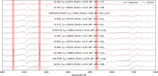
Spectra recovery for a representative set of benchmark stars with the WiFeS blue arm for |$4000 \lt \lambda \lt 5400\,$| Å at R ∼ 3000, with observed spectra in black and Cannon model spectra in red. We generate model spectra from our fully trained three-label Cannon model at the adopted (rather than best fit) benchmark labels. The vertical red bars correspond to H β, H γ, and H δ from the hydrogen Balmer series which were masked out to avoid emission features. The stars are sorted by their Gaia (BP − RP) colour to show a smooth transition in spectral features across the parameter space considered.
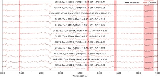
As Fig. 4, but for WiFeS red arm spectra with |$5400 \lt \lambda \lt 7000\,$| Å at R ∼ 7000. The vertical red bars (from left to right) correspond to a bad column on the WiFeS detector, atmospheric H2O absorption, H α from the hydrogen Balmer series, and O2 telluric features, all of which were masked during modelling.
This recovery is particularly impressive when considering the deviations observed in Rains et al. (2021) between MARCS and Bt-Settl (Allard, Homeier & Freytag 2011) synthetic spectra versus the same flux normalized spectra we train our Cannon model on here. In their section 4.1, in particular figs 4 and 5, they discuss 2–10 per cent flux differences between synthetic and observed spectra for several optical bands – deviations large enough to be quite obvious to the eye. We discuss these differences more quantitatively in Section 5.2.
3.4 Model validation and label recovery performance
The accuracy of a data-driven or machine learning model can only be truly determined by testing the model on unseen data – i.e. data the model was not trained upon. Ideally one would have a large enough sample to initially partition it into separate training and test sets without compromising on model accuracy. With only 103 benchmarks, however, this is not feasible for our work here, so we instead opt for a leave-one-out cross-validation approach. Under this paradigm, we train N different Cannon models on N different sets of N − 1 benchmark stars, testing each model on the Nth benchmark left out of the model. Our final reported label recovery accuracy thus consists of the medians and standard deviations of the aggregate ‘left out’ sample across all models. Labels are fit using the curve_fit function from scipy given the coefficient and scatter arrays θ and sλ from a fully trained Cannon model as described in Section 3.2.
We plot our label recovery performance in leave-one-out cross-validation for Teff, log g, and [Fe/H] in Fig. 6 for both our three- and four-label models. Similarly, Fig. 7 illustrates our stellar parameter recovery as a function of label source: Teff from interferometry, [Fe/H] from Mann et al. (2015), [Fe/H] from Rojas-Ayala et al. (2012), and [Fe/H] from F/G/K binary companions – again for our three and four parameter models, respectively. Finally, Fig. 8 shows [Ti/Fe] recovery for our four-label model. Table A1 lists the labels inferred from our fully-trained four label model in Teff, log g, [Fe/H], and [Ti/Fe] for our benchmark, noting that while these values are from the model trained on all 103 stars, our uncertainties are derived from the leave-one-out cross-validation performance standard deviations added in quadrature with the statistical uncertainties. For our four–label model, these statistical uncertainties are rather small with means 1.3 K, 0.001 dex, 0.004 dex, and 0.001 dex in Teff, log g, [Fe/H], and [Ti/Fe] respectively, meaning that our reported errors are based primarily on how well we recover our adopted set of literature benchmark labels. We adopt (and correct for) Teff, log g, [Fe/H], and [Ti/Fe] systematics and uncertainties of |$-1\pm 51\,$|K, |$0.00\pm 0.04\,$| dex and |$0.00\pm 0.10\,$| dex, and |$0.01\pm 0.06\,$| dex, respectively. We note that these uncertainties purely refer to how well our recovered parameters reproduce the adopted benchmark Teff, log g, [Fe/H], and [Ti/Fe] scales – i.e. the quality of our label transfer using the Cannon.11 It is an altogether different task – and beyond the scope of our work here – to refine these benchmark scales, with studies comparing e.g. physically realistic Teff (Tayar et al. 2022) or abundance uncertainties (via differential analysis of Solar twins, e.g. Ramírez et al. 2014) indicating that these uncertainties – including the adopted literature values for our benchmarks – are likely underestimates.
![Leave-one-out cross-validation performance for recovery of adopted labels (per Table 1) for Top: 3 label (Teff, log g, [Fe/H]) and Bottom: 4 label (Teff, log g, [Fe/H], [Ti/Fe]) Cannon models respectively. Each panel shows the median and standard deviation of the residuals computed between the adopted benchmark values and Cannon predicted equivalents, where σresid is added in quadrature with the Cannon statistical uncertainties to give our adopted label uncertainties.](https://oup.silverchair-cdn.com/oup/backfile/Content_public/Journal/mnras/529/4/10.1093_mnras_stae560/1/m_stae560fig6.jpeg?Expires=1749174622&Signature=ern7Pjc4nskXfL3sJ5K1j-PAqApVexQ-L6DZ~A-cRJ~zxB46X6INwLz64Q5p7lJQQIZDZV6sQl14GvjVZZR3DYV-lCQmiGHYk6P26gYons~wNzg-~iSaIo7GFhXBh1BS~SZLR2BbeESWzBrkfAGOqCevr04IoXyXwzSp~WYrzEsy18Vb1qDZtex9whYFlBkeb8~kbw5j3QtDI5q-4I-w1G3k4ceGgRJ7bgDgQiZA72hH7nbd-6kU36CulVJkO6UAUwmjmo2H5I1SITegd23GFswgBw9Z4Y9sSgO-Nafxqkq6TrVq~oAmPDu6UGqiS0fZYxx8DSbIm548xlV3lxGLkA__&Key-Pair-Id=APKAIE5G5CRDK6RD3PGA)
Leave-one-out cross-validation performance for recovery of adopted labels (per Table 1) for Top: 3 label (Teff, log g, [Fe/H]) and Bottom: 4 label (Teff, log g, [Fe/H], [Ti/Fe]) Cannon models respectively. Each panel shows the median and standard deviation of the residuals computed between the adopted benchmark values and Cannon predicted equivalents, where σresid is added in quadrature with the Cannon statistical uncertainties to give our adopted label uncertainties.
![Leave-one-out cross-validation performance for label recovery of literature parameter sources for Top: 3 label (Teff, log g, [Fe/H]) and Bottom: 4 label (Teff, log g, [Fe/H], [Ti/Fe]) Cannon models, respectively. Note that benchmark stars with [Fe/H] values published in multiple catalogues (e.g. both Rojas-Ayala et al. 2012 and Mann et al. 2015) are plotted in multiple panels with their own colour bars – not just the panel for the source we formally adopted. Each panel shows the median and standard deviation of the residuals computed between the adopted benchmark values and Cannon predicted equivalents.](https://oup.silverchair-cdn.com/oup/backfile/Content_public/Journal/mnras/529/4/10.1093_mnras_stae560/1/m_stae560fig7.jpeg?Expires=1749174622&Signature=JMeN6FCxNQC~xLZ6OQISqgsQmSqgZ1WqIe-ZcrSozaniPcqYWCqtvFgmHRk5bdzg9xZWQvTlq03c8hF0vd0FkEqGaWWMvpW-LICBaIY2myyhgFcB3PWNsmm8OpJuEwF5gtbubLoxDw6mKj4S0Vr9vEv~vHmfH7mBzT-UyjokNor9cIf9BwRRGSiOWac8Gc2pWgbHKU1W5pyOooDuk-LZy8VZBeSprrLNsxRX5AZo8SiUNmkT1pFPqeWMfc9qS1UVGZcXrksLF7ZhmtjSt~4IAtTyCEmofhgwiscTtf5PmdHm9By0f7KGkunYo1OfxRBdbzsPYtZhjIw0IyyEgZRxsg__&Key-Pair-Id=APKAIE5G5CRDK6RD3PGA)
Leave-one-out cross-validation performance for label recovery of literature parameter sources for Top: 3 label (Teff, log g, [Fe/H]) and Bottom: 4 label (Teff, log g, [Fe/H], [Ti/Fe]) Cannon models, respectively. Note that benchmark stars with [Fe/H] values published in multiple catalogues (e.g. both Rojas-Ayala et al. 2012 and Mann et al. 2015) are plotted in multiple panels with their own colour bars – not just the panel for the source we formally adopted. Each panel shows the median and standard deviation of the residuals computed between the adopted benchmark values and Cannon predicted equivalents.
![[Ti/Fe] leave-one-out cross-validation performance for our binary benchmarks using our 4 label (Teff, log g, [Fe/H], [Ti/Fe]) Cannon model.](https://oup.silverchair-cdn.com/oup/backfile/Content_public/Journal/mnras/529/4/10.1093_mnras_stae560/1/m_stae560fig8.jpeg?Expires=1749174622&Signature=RUJ7b79CpOpC3nwX-F6AFKge176kdlL8IpM4aOM2rP0R3YegHXAp5YRNOd8QVxtelrSfxJeuRSu3IupUHpxds6Ho04pAFYm3xJ7k~5CuMeEZKcXFMQn6rW53MzhrUsdaczSK3s9yytiFKi2GFl2Kt-OujnJPxvXTsB42PrlO5AE-BFDV5f-urPmWlOK0kq2pMgMOUl1Jeh2Vym53zNoyPjozTy7cAsxt33xR71ZAywWJ5EAuUHxvWbGjtnnRpPIcXGfaxTES-b~C~g2FEjfrttyZyMmYwbFRkDi41nrgSxSQ9RvG-Eh4BGHz9dEKiB71tSwPuOrz~GH8qOf3OT-RrQ__&Key-Pair-Id=APKAIE5G5CRDK6RD3PGA)
[Ti/Fe] leave-one-out cross-validation performance for our binary benchmarks using our 4 label (Teff, log g, [Fe/H], [Ti/Fe]) Cannon model.
Overall, our three and four label models have similar label recovery performance (as distinct from spectral recovery), with Fig. 6 showing the most significant difference between the two models being a reduced Teff systematic (|$+7.83\,$| to |$-1.42\,$| K) and scatter (|$\pm 53.97\,$| to |$\pm 51.04\,$|K) for the four label model. Given that one of the main indicators of Teff in cool dwarf atmospheres are the TiO bandheads – the characteristic ‘sawtooth’ pattern in cool optical spectra and the traditional indicator of M dwarf spectral types – this improvement is consistent with expectations given the extra constraints provided by modelling [Ti/Fe]. By contrast, however, there are no similar improvements to log g and [Fe/H] recovery when using the four label model, and we hypothesize that there are three factors at play here. The first of which is that our three label model already recovers log g and [Fe/H] at or nearly at the precision of the benchmark sample itself, meaning that further improvements would likely be marginal even in the best case. The second is that these parameters are less acutely sensitive to [Ti/Fe] or TiO absorption than Teff is, or at least have constraints from unrelated spectral features. For example, other molecules like CaH are strongly sensitive to log g and have long been used as a discriminator between traditional stellar luminosity classes like subdwarf, dwarf, and giant (e.g. Öhman 1936; Jones 1973; Mould & McElroy 1978; Kirkpatrick, Henry & McCarthy 1991; Mann et al. 2012). Thirdly is the effect of small number statistics, as our models are trained on only 103 benchmarks the influence of outliers (discussed more in subsequent paragraphs) is more significant when computing the scatter from the standard deviation of the residuals – an effect which might hide slight improvements in label recovery. When considering Fig. 7, which separates out label recovery for different literature sources, we are especially hesitant to draw firm conclusions about the differences between the two models given the smaller sample sizes – something especially acute for the binary sample – and lack of a Cannon model which models label uncertainties as we can only expect label recovery at the level of the median σ[Fe/H] of our benchmark sample. None the less, our results are consistent with the expectation that a model constraining [Ti/Fe] would be better able to recover optical cool dwarf parameters given the significant influence of TiO on optical spectra.
NLTT 10 349 (Gaia DR3 3266980243936341248), our most metal-poor star with [Fe/H] = −0.86 ± 0.04, proves a consistent outlier in cross-validation due to its uniqueness in our small benchmark sample, being roughly ∼3.7σ from our sample’s mean [Fe/H] (versus ∼2.3σ from the mean value for the second most metal poor star). Our model’s inability to accurately recover its [Fe/H] in cross-validation is a reflection on our sample size, rather than for instance a breakdown in the behaviour of cool dwarf spectra at low [Fe/H], leading to our conclusion that the Cannon is unable to accurately extrapolate far beyond the label values of the benchmarks used to initially train it.
Our Teff recovery for both models is entirely consistent with the median Teff precision of our sample (|$\pm 67\,$| K versus our |$\pm 51\,$| K here). There are similar systematics observed between the bulk and interferometric samples, which points to our adopted Teff scale being correctly calibrated to a fundamental scale, despite the challenges noted in Rains et al. (2021) with their interferometric sample having saturated 2MASS photometry.
Our log g recovery is almost–consistent to within literature uncertainties (|$\pm 0.02\,$| dex versus our |$\pm 0.04\,$| dex here), noting that our gravities are mostly from photometric |$M_{K_S}$|–M⊙ relations, and should be reliable for main sequence stars (but less accurate for unresolved binaries or stars still contracting to the main sequence). Assuming the Cannon has successfully learnt how to identify gravity through gravity sensitive spectroscopic features, observed outliers in log g could be unresolved binaries as the Cannon predicting higher gravities is consistent with underpredicted gravities from blended photometry. While cursory inspection of the spectra of these stars did not reveal any spectroscopic binaries, this hypothesis was validated once we made a RUWE cut upon the release of Gaia DR3, which removed most of the targets (i.e. observed benchmarks which no longer pass the quality cuts to appear in our work here) with aberrant log g values, improving the precision of our log g recovery from an initial |$\pm 0.06\,$| dex to the reported |$\pm 0.04\,$| dex (which itself drops to |$\pm 0.03\,$| dex were we to exclude the two most aberrant stars in the sample).
Another alternative to unresolved binaries is that the Cannon could be giving higher gravities to young stars still contracting to the main sequence as it has not been trained on such a sample. We note that Behmard et al. (2019) included a vsin i dimension to their Cannon model, but we are far less sensitive to rapid rotation with our R ∼ 7000 spectra versus their R ∼ 60 000 resolution spectra. Either of these physical explanations would serve to increase the scatter on our primarily photometric log g values, but regardless of the physical origin we have flagged those remaining benchmarks with fitted log g aberrant by >0.075 dex in Table A1 using †.
The primary motivation of our work here was to study the chemistry of our cool dwarf sample from optical spectra, something Rains et al. (2021) was unable to accomplish previously using a model-based approach using the same spectra as we do here. Instead they developed a new photometric [Fe/H] relation precise to |$\pm 0.19\,$| dex applicable to isolated main sequence stars. When compared this baseline, the ability of our Cannon model to recover [Fe/H] to ±0.10 dex represents a significant improvement, even more so given our successful recovery of [Ti/Fe] to within benchmark uncertainties (corresponding to ±0.06 dex), something we discuss in Section 5. Of note is that we achieve this [Ti/Fe] recovery with only 17/103 of our sample having measured [Ti/Fe] abundances, and the remaining 86/103 stars having [Ti/Fe] predictions informed by Galactic chemo-dynamic trends. This clearly demonstrates both (a) the strength of the [Ti/Fe] signal in optical spectra, and (b) the ability of the Cannon to learn strong features, and points to greater precisions being possible with larger benchmark samples. When considering our 4 label model, we note that our [Fe/H] recovery is nearly consistent with the uncertainties of the Mann et al. (2015) sample (our largest single source of [Fe/H], |$\pm 0.08\,$| dex versus our |$\pm 0.09\,$| dex), and better than the quoted uncertainties for the Rojas-Ayala et al. (2012) sample (our second largest source of [Fe/H], |$\pm 0.12\,$| dex versus our |$\pm 0.10\,$| dex), suggesting that their uncertainties are overestimated.
4 COOL DWARF PHYSICAL MODEL SPECTRA AND [X/FE]
To complement our discussion of data-data-driven flux recovery and cool dwarf chemistry, we now turn to a grid of physical models for comparison. More specifically, in this section we set out to study the impact of [X/Fe] on model cool dwarf continuum normalized spectra for the wavelength range covered by our WiFeS spectra.
4.1 Sensitivity of MARCS pseudo-continuum to [X/Fe]
To better understand the physics of cool dwarf atmospheres, as well as guide our interpretation of the results and performance of our Cannon model, here we conduct a pilot investigation into the influence of atomic abundances on cool dwarf spectra using a bespoke grid of MARCS spectra. As in Nordlander et al. (2019), our 1D LTE MARCS grid12 was computed using the TURBOSPECTRUM code (v15.1; Alvarez & Plez 1998; Plez 2012) and MARCS model atmospheres (Gustafsson et al. 2008). The spectra were computed with a sampling resolution of |$1\,$|kms−1, corresponding to a resolving power of |$R{\sim }3\, 00\, 000$|, with a microturbulent velocity of |$1\,$|kms−1. We adopt the solar chemical composition and isotopic ratios from Asplund et al. (2009), except for an [α/Fe] enhancement that varies linearly from [α/Fe] = 0 when |$\rm [Fe/H] \ge 0$| to [α/Fe] = +0.4 when |$\rm [Fe/H] \le -1$|. We use a selection of atomic lines from VALD3 (Ryabchikova et al. 2015) together with roughly 15 million molecular lines representing 18 different molecules, the most important of which for this work are CaH (Plez, private communication), MgH (Kurucz 1995; Skory et al. 2003), and TiO (Plez 1998, with updates via VALD3). Finally, we note that while this suite of models has issues reproducing cool dwarf optical fluxes, likely due to missing opacities or incomplete line lists (see Rains et al. 2021 for more information), the input physics should still be more than sufficient for qualitative analysis.
We say ‘bespoke grid’ because of the limited parameter space covered: the grid has three Teff values (3000, 3500, 4000 K) two log g values (4.5, 5.0), and solar values of [Fe/H] and [α/Fe] (0.0). While this might seem limiting, the strength of this grid comes from the added abundance dimensions, with each of C, N, O, Na, Mg, Al, Si, Ca, Ti, and Fe being able to be individually perturbed13 by |$\pm 0.1\,$| dex from the solar value. Thus, while the modelled star is broadly solar in composition, one can inspect the influence of small variations in abundance in isolation on optical fluxes where the pseudo-continuum position is strongly dependent on molecular absorption.
Fig. 9 shows the result of perturbing the abundances of C, O, and Ti – the three most influential elemental abundances in cool atmospheres – as well as the bulk metallicity [M/H] from |$-0.1\,$| to |$+0.1\,$| dex for the wavelengths covered by our WiFeS spectra at three different Teff values. C, O, Ti, and [M/H] all have a significant – and mostly similar – impact on pseudocontinuum placement, with this similarity indicating the degenerate nature of these parameters. Notably C has the opposite sign to O, Ti, and [M/H], which we suggest relates to CO formation. While CO does not absorb at optical wavelengths it is, however, ‘energetically favourable’ (Veyette et al. 2016) – for a lower C abundance there is a greater ‘relative’ abundance of O available to form other molecules like TiO or H2O. At |$T_{\rm eff}=3000\,$| K, wavelengths longer than |${\sim }4500\,$| Å see fractional change in flux of ∼20 per cent for C and [M/H], but closer to ∼40 per cent for Ti and O – likely due to the dominance of TiO. This effect diminishes with increasing temperature, though the pseudo-continuum can still change at the ∼5–10 per cent level – more than enough to complicate the measurement of equivalent widths via traditional spectroscopic analysis techniques. The very bluest wavelengths (below |${\sim }4 300\,$| Å) show a reduced influence from C, O, and TiO, potentially indicating that spectra in these regions would be less subject to degeneracies when fitting for the bulk metallicity. While the region between ∼4100–|$4200\,$| Å (likely due to SiH in our synthetic spectra due to our choice of line list,14 see Fig. 10) shows reduced influence from Ti as compared to C, O, and [M/H], on the whole it otherwise appears very difficult to disentangle the contributions from each element and the bulk metallicity.
![Sensitivity of cool dwarf MARCS model fluxes to variations in abundances for elements present in dominant molecular absorbers (C, O, and Ti) over the WiFeS wavelength range, as demonstrated with three different sets of solar [M/H] spectra (from top to bottom) with Teff and log g: $3000\,$K and 5.0; $3500\,$K and 4.75; $4000\,$K and 4.65. The upper panel of each plot is the continuum normalized synthetic MARCS model spectra (model continuum level at 1.0) at Solar [M/H] and a Solar abundance pattern. The bottom panel shows the fractional change in continuum normalized flux when changing a single abundance from +0.1 to $-0.1\,$ dex of the Solar value, as well as the bulk metallicity perturbed by the same amount for comparison. Note that the flux change from C has the opposite sign to O and Ti and as such has been multiplied by −1 for better comparison, and that the y-axis scale is different for each panel.](https://oup.silverchair-cdn.com/oup/backfile/Content_public/Journal/mnras/529/4/10.1093_mnras_stae560/1/m_stae560fig9.jpeg?Expires=1749174622&Signature=AfgH2wZ3PH2ry7BLDj~UBm7a1iXjax1l1VnsTlGQ6Q4gDmQdu9GaOLVo9k5~2YvyQ536Qjcgy-1c6ihwUumixnm6q7UO3A1Ymz3VmWAq1~KVq1GBChqzrY-JdLwUBcpCDWIxwHeTJB~nbHoE3-K7pksYEl35YQLAIevzd-q0ElPPwFRAUVg91d0dAtRi3CzYoz3A~zEhBYsGd6zLiIct~wjsQuZWpr4pHQZR5UlfY4v158PQJ78BDNkwCZea9upPYEU3wC04sHvbzXlk3Q~huN4UZvRnjzdp99z~jWjr-E~FjZFIPJb4BkXqw2~DyAMC44BEqjtTHO1d0xpKNpsYCg__&Key-Pair-Id=APKAIE5G5CRDK6RD3PGA)
Sensitivity of cool dwarf MARCS model fluxes to variations in abundances for elements present in dominant molecular absorbers (C, O, and Ti) over the WiFeS wavelength range, as demonstrated with three different sets of solar [M/H] spectra (from top to bottom) with Teff and log g: |$3000\,$|K and 5.0; |$3500\,$|K and 4.75; |$4000\,$|K and 4.65. The upper panel of each plot is the continuum normalized synthetic MARCS model spectra (model continuum level at 1.0) at Solar [M/H] and a Solar abundance pattern. The bottom panel shows the fractional change in continuum normalized flux when changing a single abundance from +0.1 to |$-0.1\,$| dex of the Solar value, as well as the bulk metallicity perturbed by the same amount for comparison. Note that the flux change from C has the opposite sign to O and Ti and as such has been multiplied by −1 for better comparison, and that the y-axis scale is different for each panel.
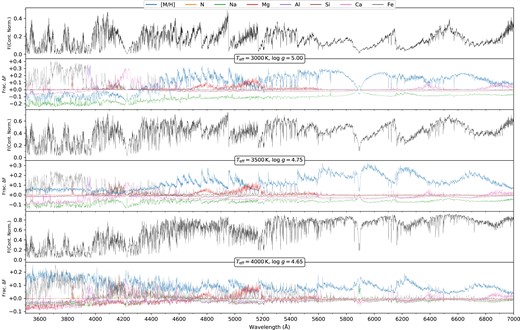
As Fig. 9, but for elements present in non-dominant molecular absorbers (N, Na, Mg, Al, Si, Ca, and Fe).
Fig. 10 is the same, but for N, Na, Mg, Al, Si, Ca, and Fe instead. While none of these reach the significance of C, O, and Ti, being generally much more limited in the wavelength regions they affect, everything except N has at least one spectral region with a flux change of ∼5−10 per cent. Of note is that, outside of a number of strong lines, the influence of Fe is mainly below ∼4000 Å. This means that our Cannon model – as well as other optical [Fe/H] relations – are likely not actually sensitive to Fe spectral features directly when trained upon [Fe/H], rather how the shape of the pseudo–continuum correlates with [Fe/H]. We attribute the surprisingly large influence Na has on flux (at the ∼5–20 per cent level) to it being an electron donor, rather than being directly involved in atomic or molecular absorption itself.
Collectively, even qualitative analyses like this allow insight into the sensitivity of different wavelength regions to varying elemental abundances to guide spectral analysis. Optical wavelengths clearly contain a wealth of chemical information, but limitations with current models in the cool dwarf regime and the parameters varied in model grids make this difficult to exploit using traditional methods.
5 DISCUSSION
5.1 Model scatter and wavelength label sensitivity
Now with some theoretical insight into how sensitive optical cool dwarf fluxes are to variations in abundance, we can begin to assess the performance of our Cannon model in terms of how well it recovers these fluxes. The Cannon attempts to parametrize the flux of each spectral pixel as a function of the adopted stellar labels, in our case Teff, log g, [Fe/H], and [Ti/Fe]. Also inherent to the Cannon model is a noise term (see equation 5) associated with each spectral pixel, which accounts for the fact that a) the training spectra are not known to arbitrarily high precision and thus have an associated flux uncertainty, and (b) a scatter term to account for remaining flux variation unable to be parametrized as a function of the adopted labels with our adopted polynomial order. Broadly speaking, we would expect spectral pixels associated with strong atomic absorption features for atoms other than Fe or Ti to be poorly modelled by the Cannon as it does not have the constraints to properly learn these features. Similarly, since the entire optical region is affected by molecular absorption for cool stars, we in general expect a higher baseline model scatter for all pixels, peaking where atomic or molecular features from elements unconstrained by our purely [Fe/H]–[Ti/Fe] chemical model dominate.
One important caveat to keep in mind before we begin assigning flux sensitivities or model scatter to being a function of stellar chemistry are observational factors about our spectra or benchmark sample that could cause similar effects. The first of these is the SNR of our data, which is not uniform as a function of wavelength or Teff. In general, the warmer stars in our sample have higher SNR spectra from the WiFeS blue arm, with the coolest stars by comparison having much lower SNR in the blue – the very reason our Cannon model begins at |$4000\,$| Å rather than covering the full extent allowed by the B3000 grating. The second effect is that of spectral resolution, with B3000 pixels having lower resolving power than their R7000 grating counterparts on the red arm. This could result in adjacent spectral features, which might be resolved at R ∼ 7000, being blended at R ∼ 3000 and being accordingly more complex for the Cannon to parametrize as compared to the same information spread across two separate pixels. Finally, given the relatively small training sample, there exists the possibility of edge effects near the edge of the parameter space where the model is more poorly constrained – something which could also increase model scatter.
With that introduction and caveating out of the way, Figs 11 and 12 present benchmark spectra, pixel sensitivity, and model scatter for the B3000 and R7000 wavelength regions, respectively, and Table 2 offers a counterpart summary for each term in the label vector θN. From top-to-bottom, each plot shows the normalized benchmark stellar spectra (labelled with prominent atomic features); spectral pixel sensitivity to Teff, log g, [Fe/H], and [Ti/Fe] in the form of the linear Cannon coefficients; quadratic Cannon coefficients; cross-term Cannon coefficients; and the Cannon model scatter for each spectral pixel for our 3 and 4 label models (also labelled with prominent atomic features). For the purposes of comparison, note that the y-axis scale for the Cannon scatter panels are the same for both plots.
![Four label Cannon model pixel sensitivity to stellar labels and model scatter for WiFeS B3000 spectra with prominent atomic absorption features of Ca i, Ti i, and Fe i labelled (EW$\gt 400\,$ m Å, calculated for $T_{\rm eff}=3 500\,$ K, log g = 5.0, [Fe/H] = 0.0). Panel 1: Normalized B3000 spectra of stellar benchmarks used to train the model, where darker coloured spectra correspond to cooler stars. As before, the shaded red regions correspond to stellar emission, telluric absorption, or bad pixels. Panel 2: First order θ coefficients for each of the stellar labels (Teff, log g, [Fe/H], and [Ti/Fe]). The further each coefficient is from 0, the more sensitive the flux in a given spectral pixel is to a specific label. Panel 3: As Panel 2, but for second order θ coefficients. Panel 4: As Panel 2 and 3, but for cross-term θ coefficients. Panel 5: Cannon modelled scatter for each spectral pixel for both our 3 and 4 label Cannon models, where higher values indicate that the adopted stellar labels are increasingly insufficient to completely parametrize the stellar flux. The same absorption features as before are overplotted.](https://oup.silverchair-cdn.com/oup/backfile/Content_public/Journal/mnras/529/4/10.1093_mnras_stae560/1/m_stae560fig11.jpeg?Expires=1749174622&Signature=gSs0~orRcUMsEnQpu~pRBzVrOo9bQcwMynKjChicSVQMjMaJIHmV~syWX~baAPquaanewZO8zpxNF1dEDcGGXUFiEFq9UGc2f9IL4LI6FOKg9FjeoWS-HFZMOd8SbrnK8x0crRJ9oZzmfayX8EePFK4Lv-YzpXwhovuweifygw6dHlm3Y1ddsTsMAjw219dvDzLQnhJtSGbhylg1YV47UzTEpf0I8v8N4RUyUgpxu0gTib1OEZ8NZbBaAUQEvGZk-zAQNzYHDoHHBrVzgB67V~Ez18NPkQqXdwTYyenKM9GQXACBRogQ9M~12DHJbWmPS3M300Jsyu-X4Yry9Q6EVA__&Key-Pair-Id=APKAIE5G5CRDK6RD3PGA)
Four label Cannon model pixel sensitivity to stellar labels and model scatter for WiFeS B3000 spectra with prominent atomic absorption features of Ca i, Ti i, and Fe i labelled (EW|$\gt 400\,$| m Å, calculated for |$T_{\rm eff}=3 500\,$| K, log g = 5.0, [Fe/H] = 0.0). Panel 1: Normalized B3000 spectra of stellar benchmarks used to train the model, where darker coloured spectra correspond to cooler stars. As before, the shaded red regions correspond to stellar emission, telluric absorption, or bad pixels. Panel 2: First order θ coefficients for each of the stellar labels (Teff, log g, [Fe/H], and [Ti/Fe]). The further each coefficient is from 0, the more sensitive the flux in a given spectral pixel is to a specific label. Panel 3: As Panel 2, but for second order θ coefficients. Panel 4: As Panel 2 and 3, but for cross-term θ coefficients. Panel 5: Cannon modelled scatter for each spectral pixel for both our 3 and 4 label Cannon models, where higher values indicate that the adopted stellar labels are increasingly insufficient to completely parametrize the stellar flux. The same absorption features as before are overplotted.
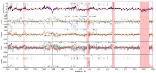
As Fig. 11, but for WiFeS R7000 spectra.
Comparison of standard deviations computed for each θ term – offset, first order, second order, and cross-term – for both our 3 and 4 label Cannon models. Larger values indicate a given coefficient (and thus the associated stellar parameter/s) is a more important term in modelling stellar fluxes.
| θ3Label | |$\sigma _{\theta _N}$| | ||
|---|---|---|---|
| B3000 | R7000 | All | |
| 1 | 0.151 | 0.110 | 0.126 |
| Teff | 0.036 | 0.035 | 0.035 |
| log g | 0.019 | 0.016 | 0.017 |
| [Fe/H] | 0.013 | 0.008 | 0.010 |
| |$T_{\rm eff}\, ^2$| | 0.016 | 0.009 | 0.012 |
| |$\log g\, \times \, T_{\rm eff}$| | 0.034 | 0.019 | 0.026 |
| |${\rm [Fe/H]}\, \times \, T_{\rm eff}$| | 0.012 | 0.009 | 0.010 |
| log g2 | 0.028 | 0.014 | 0.020 |
| |${\rm [Fe/H]}\, \times \, \log g$| | 0.016 | 0.010 | 0.012 |
| [Fe/H]2 | 0.005 | 0.004 | 0.004 |
| θ4Label | |$\sigma _{\theta _N}$| | ||
| B3000 | R7000 | All | |
| 1 | 0.151 | 0.110 | 0.126 |
| Teff | 0.038 | 0.037 | 0.037 |
| log g | 0.019 | 0.017 | 0.018 |
| [Fe/H] | 0.017 | 0.009 | 0.013 |
| [Ti/Fe] | 0.014 | 0.007 | 0.010 |
| |$T_{\rm eff}^2$| | 0.016 | 0.009 | 0.012 |
| |$\log g\, \times \, T_{\rm eff}$| | 0.034 | 0.021 | 0.026 |
| |${\rm [Fe/H]}\, \times \, T_{\rm eff}$| | 0.025 | 0.011 | 0.017 |
| |${\rm [Ti/Fe]}\, \times \, T_{\rm eff}$| | 0.028 | 0.011 | 0.019 |
| log g2 | 0.028 | 0.015 | 0.020 |
| |${\rm [Fe/H]}\, \times \, \log g$| | 0.032 | 0.012 | 0.021 |
| |${\rm [Ti/Fe]}\, \times \, \log g$| | 0.035 | 0.011 | 0.022 |
| [Fe/H]2 | 0.011 | 0.007 | 0.008 |
| |${\rm [Ti/Fe]}\, \times \, {\rm [Fe/H]}$| | 0.018 | 0.011 | 0.014 |
| [Ti/Fe]2 | 0.010 | 0.007 | 0.008 |
The model scatter in the blue is on average higher than in the red, which is consistent with both a higher contribution from unmodelled atomic absorption at bluer wavelengths, and the aforementioned lower spectral resolution of our B3000 spectra. We see a reduction in the median scatter value across all pixels by |${\sim }7.2\,$| per cent when switching from a three label to a four label model, which gives some hint as to the improved explanatory power of adding [Ti/Fe] as a label when attempting to reproduce observed spectra.
Table 2 lists the standard deviation |$\sigma _{\theta _N}$| for each coefficient in our coefficient vector θN – linear, quadratic, and cross-term in each label – for both WiFeS wavelength ranges, and for each of our two Cannon models. Larger values of |$\sigma _{\theta _N}$| correspond to the terms that are important for describing the largest-scale changes in the spectrum, for instance the linear and quadratic Teff and log g terms for describing TiO bandheads. Values for all labels are uniformly larger in the blue versus the red, which again is consistent with the lower spectral resolution and higher atomic contribution in the blue. The cross-terms in particular give insight into the correlations between each label, and it will be interesting to see what would happen were we to add further [X/Fe] dimensions in follow-up work. Finally, of particular note is how important log g is as a label in linear, quadratic, and cross-terms – despite the fact it is often determined using photometry and was the label we put the least effort into sourcing literature values for. That said, for stars on the main sequence (i.e. the bulk of our sample bar the aforementioned outliers) log g is going to be well – or entirely – correlated with Teff and [Fe/H] so it likely is not truly an independent label.
There are numerous strong lines of Ca, Ti, Cr, and Fe in the spectrum (among other elements) which are clearly associated with many of the large ‘spikes’ in model scatter. At this resolution we do not just expect a contribution from isolated strong lines, but also closely bunched multiplets which, while blended, still observably affect flux. As expected, there are many more atomic features towards bluer wavelengths – the exact regions where models are the least reliable, and cool dwarfs the faintest. None the less, this points once more to the sheer amount of chemical information present at optical wavelengths for these stars, most of which is also inaccessible under our current Cannon model formalism.
Our present Cannon model assumes that the flux of every spectral pixel depends on Teff, log g, [Fe/H], and [Ti/Fe] – the entire set of modelled stellar labels. While this is physically reasonable in the optical where much of the spectral information for these labels is contained in broad molecular features spanning a large range in wavelength, this assumption ceases to be valid when trying to model the abundances for elements whose primary influence is present only as discrete atomic lines. Thus, to better represent known physics it is more reasonable to implement a Cannon model with regularization whereby coefficients are actively encouraged to take on values of zero. Casey et al. (2016) demonstrated such an approach successful in modelling the full suite of APOGEE stellar parameters (Teff, log g, and 15 abundances: C, N, O, Na, Mg, Al, Si, S, K, Ca, Ti, V, Mn, Fe, Ni), and we are hopeful that following their approach in the future would allow us to add additional [X/Fe] dimensions to our Cannon model.
Finally, with reference back to Figs 9 and 10, it is possible to qualitatively compare model molecular absorption with increased Cannon model scatter sλ (noting that we cannot expect a 1:1 match in light of known model spectra difficulties reproducing optical fluxes). Two regions of increased scatter seem to correspond with Ca-associated features (likely CaH) |$4100\!-\!4300\,$| Å (the region of largest scatter in the blue) and |$6\, 100{\!-\!}6\, 150\,$| Å (Ca i), though there are also relatively strong [Si/H] and [Fe/H] features in the former region. The Na doublet region (|$5800{\!-\!}6000\,$| Å) has the most scatter in the red, but it is difficult to ascribe this to Na alone. Curiously, |$4\, 700-5200\,$| Å is the region where we expect Mg to have the largest impact, but the scatter is small compared to the aforementioned regions. While it is difficult to discuss this quantitatively with our existing model, it would be illustrative to revisit this with a future version of the Cannon with regularization and a broader set of chemical labels.
5.2 Data-driven versus physical model flux recovery
Given the good performance of our Cannon model in recovering optical fluxes, it is illustrative to perform a comparison between data-driven and physical model spectra. For this comparison, we treat our Cannon–produced spectra essentially as a self-consistent and interpolatable proxy for the observed spectra which, among other things, removes the influence of SNR or artefacts present in any single observed spectrum. Fig. 13 shows a comparison between our 3 label Cannon model in Teff, log g, and [Fe/H] and the equivalent MARCS model spectra for the same set of benchmarks stars and adopted benchmark parameters presented in Figs 4 and 5 (again using the three–label model to avoid interpolating the MARCS grid in [Ti/Fe]). Alongside this is Fig. 14 which shows the percentage flux difference between the Cannon and MARCS spectra for all 103 benchmark stars (spanning the ranges 1.7 < (BP − RP) < 3.8 and 4.55 < log g < 5.20). Our MARCs spectra were generated using the same grid used for Rains et al. (2021), and normalized using the same normalization formalism applied to our observed spectra as described in Section 3.1.
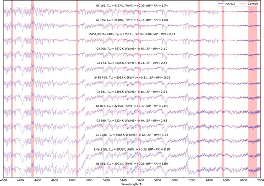
Comparison between our fully-trained 3 label Cannon versus MARCS model spectra for a representative set of benchmark stars for |$4000 \lt \lambda \lt 7000\,$| Å at R ∼ 3000−7000, with Cannon model spectra in red and MARCS model spectra in blue. Both the MARCS and Cannon spectra have been generated at our adopted benchmark labels, rather than our fitted labels. The vertical red bars (from left to right) correspond to H δ, H γ, H β, a bad column on the WiFeS detector, atmospheric H2O absorption, H α, and O2 telluric features, all of which were masked out during modelling. The stars are sorted by their Gaia (BP − RP) colour to show a smooth transition in spectral features across the parameter space considered.
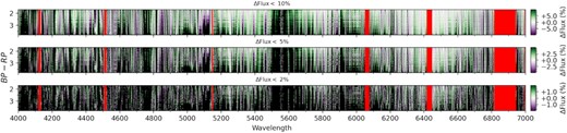
Percentage flux difference between our fully trained 3 label Cannon versus MARCS model spectra for all 103 cool dwarf benchmarks, again sorted by Gaia DR3 (BP − RP) colour. From top to bottom the panels show wavelengths where the percentage flux difference is <10 per cent, <5 per cent, and <2 per cent, respectively. Each panel has its own colour bar, where white regions indicate a good match between the Cannon and MARCS spectra (ΔFlux ≈ 0), with the colour getting progressively darker green (ΔFlux > 0) or purple (ΔFlux < 0) as the match worsens. Any wavelength region with a percentage flux difference beyond the 10 per cent, 5 per cent, or 2 per cent levels, respectively, is set to black, and the vertical red bars are again global masked telluric/emission/bad pixel regions. Note that these percentage differences only apply to our normalized spectra, and not unnormalized flux-calibrated spectra, but they remain a useful metric for quantifying the accuracy of physical models like MARCS. These benchmarks span the parameter ranges 1.7 < (BP − RP) < 3.8 and 4.55 < log g < 5.20.
Takeaways from this comparison are as expected from previous studies: performance is worse at bluer wavelengths and cooler temperatures. A few more detailed observations are as follow:
The best matching wavelength region is the few 100 Å wide region surrounding H α (nominally |${\sim }6 400$|–|$6 800\,$| Å though even this gets worse towards mid-M spectral types).
The wings of the Na d feature are consistently poorly reproduced by MARCS, even for the warmest stars in our sample.
Discrepancies at blue wavelengths are obvious for even the warmest stars in our sample, and continue to get (sometimes dramatically) worse with cooler temperatures.
While the positions of TiO bandheads are well matched, their fluxes are not, likely posing problems for temperature or spectral-type determination.
Several broad absorption features (e.g. |${\sim }4 400$|–|$4500\,$| and ∼5500–|$5600\,$| Å) are not reproduced in the MARCS spectra – indicative of missing opacity sources.
We suspect the mismatch between |$4000 \rm \,{and}\,4500\,$| Å is caused by a spectral depression centred on the |${\sim }4227\,$| Å neutral Ca resonance line that is poorly reproduced by MARCS. This feature – long known in the literature (e.g. Lindblad 1935; Vyssotsky 1943) – was recently investigated in detail by Jones et al. (2023), who conclude the mismatch between models and observations is due to a ‘lack of appropriate treatment of line broadening for atomic calcium’. We direct interested readers to this paper and the references within for more information.
This is not a perfect comparison, since we cannot control for the effect of elemental abundance variations which strongly affect optical fluxes. Where our MARCS models have a uniform scaled solar abundance pattern – critically uniform C, O, and Ti abundances – our Cannon model is trained on stars from the Solar neighbourhood that will instead show a spread in abundances. Further, our normalization formalism is likely not robust to spectra as dramatically different as the Cannon versus MARCS blue spectra are due to incomplete line lists or opacities in the latter. None the less, even a qualitative comparison is illustrative the degree to which current generation model optical fluxes at low and medium resolution are a poor match to observations, and we advise caution when considering a purely model-based approach when working with optical spectra of cool dwarfs.
5.3 Comparison with previous data-driven studies
Now we turn to putting our work in the broader context of other data-driven studies of cool dwarfs, with a broad overview shown in Table 3. While the studies referenced span a range of data-driven algorithms, spectroscopic data sets, and modelling choices, we ultimately find it useful to evaluate them against two metrics that underpin much data-driven work in astronomy: label transfer and domain exploration.
Comparison of previous data driven analyses on cool dwarfs.
| Study | Method | Data | R | λ | Teff | Ntrain | Label source | Labels | |$\sigma _{T_{\rm eff}}$| | σ[Fe/H] |
|---|---|---|---|---|---|---|---|---|---|---|
| nm | K | K | ||||||||
| Behmard et al. (2019) | Cannon | CPSa | |$60\, 000$| | 499−610 | |$3\, 000-5\, 200$| | 141 | NIRb, Ic | Teff, R⋆, [Fe/H], vsin i | 68 | 0.08 |
| Birky et al. (2020) | Cannon | APOGEEd | |$22\, 500$| | |$1\, 500-1\, 700$| | |$2\, 860-4\, 130$| | 87 | NIR | Teff, [Fe/H] | 77 | 0.09 |
| Galgano et al. (2020) | Cannon | LAMOSTe | |$1\, 800$| | 450 − 750 | |$3\, 000-4\, 100$| | 1 388 | TCDf | Teff, R⋆, M⋆, L⋆ | 110 | – |
| Maldonado et al. (2020) | PCAg | HARPSh | |$1\, 000-2\, 000^i$| | 534 − 691 | |$3\, 100-4\, 100$| | 19 | Bj | [Fe/H], [X/H] × 14k | – | 0.04 |
| Li et al. (2021) | SLAMl | LAMOST | |$1\, 800$| | 369 − 910 | |$2\, 800-4\, 500$| | 3 785 | APOGEE | Teff, [M/H] | 48 | 0.13 |
| This Work | Cannon | WiFeS | |$3\, 000/7\, 000$| | 400 − 700 | |$2\, 900-4\, 200$| | 103 | NIR, B, I | Teff, log g, [Fe/H], [Ti/Fe] | 51 | 0.10 |
aCalifornia Planet Search (CPS; Howard et al. 2010); bcool dwarfs with [Fe/H] from NIR empirical relations; ccool dwarfs with interferometric Teff and R⋆; dApache Point Galactic Evolution Experiment (APOGEE, Majewski et al. 2017); ethe LAMOST Survey (Cui et al. 2012); fTESS Input Catalogue ID (Muirhead et al. 2018); gPrincipal Component Analysis; hHARPS High-Accuracy Radial velocity Planetary Searcher (HARPS; Mayor et al. 2003); iConvolved with a Gaussian of width 12 nm to smooth from HARPS native resolution of R ∼ 115000 down to 1000 ≲ R ≲ 2000; j[Fe/H] or [X/H] from cool dwarfs in a F/G/K–K/M binary system; kAbundances for C, Na, Mg, Al, Si, Ca, Sc, Ti, V, Cr, Mn, Co, Ni, and Zn; lStellar LAbel Machine (SLAM; Zhang, Liu & Deng 2020), which implements the Support Vector Machine (SVM) machine learning algorithm.
The goal of label transfer is to quickly and precisely propagate a smaller set of potentially computationally expensive labels to some other, often larger, set of data. This might allow the transfer of elemental abundances from high-resolution spectroscopic surveys like APOGEE to their low-resolution counterparts like LAMOST (e.g. Ho et al. 2016; Wheeler et al. 2020), enable putting stellar parameters from distinct surveys on the same scale to enable cross-survey comparison (see e.g. comparing GALAH and APOGEE, Nandakumar et al. 2022), or simply for computational efficiency due to the relative speed of data-driven methods versus more traditional modelling approaches (see e.g. GALAH DR2, Buder et al. 2018). Of note is that label transfer – however precise – also transfers any systematics or quirks from the original sample.
While all data-driven studies involve some level of label transfer, not all are – or need be – interested in domain exploration, where the goal is to better physically characterize a given parameter space and ideally learn something new or exploitable. A specific example of this is Ness et al. (2016) using the Cannon to recover spectroscopic red giant masses – historically an extremely challenging task – based on mass-dependent dredge-up signatures present in the CN absorption features of APOGEE spectra. In the case of cool dwarfs, domain exploration generally means attempting to overcome model limitations, account for Teff–chemistry degeneracies, and ideally gaining insight into the complex molecular physics governing their atmospheres.
Collectively, the studies cited in Table 3 – Behmard et al. (2019), Birky et al. (2020), Galgano et al. (2020), Maldonado et al. (2020), and Li et al. (2021) – demonstrate data-driven label transfer for cool dwarfs across a range of different wavelengths and spectroscopic resolutions. From these studies, it is clear that the inability to continuum normalize cool dwarf spectra in any physically meaningful way does not appear to be a huge impediment to precise label transfer with data-driven models, which is fortunate for the potential of the method. That said, the accuracy15 of the transferred labels depend strongly upon the training sample used and the source of its labels, with each study also taking a different approach when it comes to domain exploration. In the next three subsections, we put our work in context with these studies as we evaluate the state of the field for data-driven studies of cool dwarfs.
5.3.1 Behmard et al. (2019) and Birky et al. (2020)
Behmard et al. (2019) and Birky et al. (2020) both use the Cannon trained on small, but high-resolution, training sample of benchmark stars primarily drawn from Mann et al. (2015). Their resulting [Fe/H] uncertainties prove consistent with the fundamentally calibrated Mann et al. (2015) sample, while their Teff values are marginally less precise. This is the opposite Teff trend to what we observe with our results, where instead our values are consistent with literature uncertainties. We believe this discrepancy is a function of both spectral resolution and wavelength coverage, rather than inherent differences in our respective Cannon models. Our broader wavelength coverage – enabled by our medium-resolution spectra – encompasses a greater number of highly-temperature sensitive molecular features like optical TiO bandheads, something less present in the shorter optical range covered by the HIRES spectra from Behmard et al. (2019), or the IR APOGEE spectra of Birky et al. (2020). On the other hand, their higher spectral resolution gives them access to many more unblended atomic features to use as [Fe/H] indicators, features which in the IR are also less affected by degeneracies imposed by molecular absorption.
Using the California Planet Search (CPS) HIRES sample, Behmard et al. (2019) trains their Cannon model on a much wider temperature range (|$3000 \lt T_{\rm eff} \lt 5200\,$| K range than the other studies. This appears to have resulted in larger Teff residuals at cooler temperatures, potentially indicating that a given Cannon implementation struggles to model the molecule dominated spectra of cool stars at the same time as the more ‘regular’ spectra of their solar-type counterparts. The implication being that, short of a more complex Cannon model, it is likely best to restrict oneself to modelling the two paradigms separately – something our early prototyping with the broader range of stars from Rains et al. (2021) supports.
Our results at medium resolution and moderate SNR bear out the prediction from Behmard et al. (2019) using convolved and degraded HIRES spectra that the Cannon continues to function effectively across a range of spectral resolutions and SNRs. In an attempt to prevent overfitting, they also implemented a regularized Cannon model that yielded no gain in label prediction. Their hypothesis, similar to our discussion in Section 5.1, is that regularization is unnecessary where each stellar label affects each spectral pixel, but will become more important for models extended to include elemental abundances where a given abundance might only affect a smaller set of spectral pixels.
Birky et al. (2020) takes advantage of the Cannon being an interpretable machine learning model, and uses the first order model coefficients to identify [Fe/H] sensitive atomic or molecular features in their APOGEE spectra – the most significant of which they make publicly available. While we see similar sensitivity when interpreting our Cannon implementation, we do not report a specific list of features as in our spectra they are both more likely to be blended and outweighed in significance compared to the ever-present molecular absorption. Additionally, while they take the time to analyse their fundamentally calibrated cool dwarf [Fe/H] propagated to the broader APOGEE sample in terms of Galactic dynamic, we leave such work until we are able to derive more detailed abundances for our (much smaller) sample of stars.
Importantly, by putting their stars on a fundamentally calibrated scale, Birky et al. (2020) are able to reveal both Teff and [Fe/H] systematics in the stellar parameters reported by APOGEE. While they do not undertake a detailed analysis, they attribute these discrepancies to incomplete line lists or opacities in the stellar models used by ASPCAP (APOGEE Stellar Parameters and Chemical Abundances Pipeline; García Pérez et al. 2016), resulting in systematically biased fits as the pipeline attempts to optimize the continuum level in lieu of the missing features. This result is significant, as it hints at the danger of naively trusting cool dwarf parameters produced by generalist pipelines – something not appropriately considered by Li et al. (2021) when propagating APOGEE stellar labels to LAMOST spectra (see discussion in Section 5.3.3).
5.3.2 Maldonado et al. (2020)
Using a Principal Component Analysis (PCA) and Bayesian based approach in conjunction with F/G/K–K/M binary benchmarks Maldonado et al. (2020) was able to recover a suite of 14 elemental abundances for their cool dwarf sample – the largest set of abundances to-date using a data-driven framework. Their method used HARPS spectra of 16 binary benchmarks convolved to a resolution of R ∼ 1000 − 2000, with the training sample selected to best match the metallicity distribution of nearby (|$\lt 70\,$|pc) and kinematically similar F/G/K stars. While they do not undertake leave-one-out cross-validation as we do here, they validate their approach statistically by comparing abundances trends between K/M dwarfs and F/G/K stars, and methodologically by applying the technique to F/G/K stars to check for overfitting.
While the principal difference between our two approaches is of course the technique – PCA versus the Cannon – there is also the difference in size between our two training samples. Although our binary benchmark sample is similar in size, 17 stars versus their 16 stars, we have a much larger sample of Teff and secondary [Fe/H] benchmarks that serve to more robustly anchor our temperature and metallicity scales over a wider parameter space. Maldonado et al. (2020) notes that only three stars in their training sample have [Fe/H] |$\lt 0.1\,$| dex, and aimed to address this by matching the [Fe/H] distributions of their training sample with the Solar neighbourhood F/G/K star sample. By comparison, six of our binary benchmarks – and roughly a third of our sample overall – have [Fe/H] below this threshold. Additionally, it is unclear to the extent that their approach is sensitive to Teff − chemistry degeneracies and how this affects their parameter recover, as this is something they do not discuss. Despite these limitations, they demonstrate clear recovery of their selected set of abundances – a remarkable achievement which points to the density of chemical information in optical spectra able to be retrieved when relying on a carefully considered set of benchmark stars.
Of their recovered abundances, it is interesting that both Ca and Mg show a comparatively large scatter as both these elements, and their derived molecules in CaH and MgH, respectively, have a substantial number of absorption features in the optical. Hopefully, follow-up work from both Maldonado et al. (2020) with PCA, and our work with the Cannon, can investigate whether this is astrophysical or sample-related in nature. It is, however, extremely encouraging to see that both C and Ti show much better recoveries given the extent both affect optical fluxes (per our discussion in Section 5.1).
Finally, in terms of the merits between our respective models, it seems clear that PCA is both more effective and computationally less complex when it comes to dimensionality reduction versus our Cannon model without regularization. However, the Cannon – being a generative model – remains the more interpretable approach, and we are better able to investigate label sensitivity as a function of wavelength and compare back to theoretical models. As such, it would be illustrative to apply both approaches to the same data set to better compare, contrast, and capitalize on the respective advantages of each model in the pursuit of understanding the chemistry of cool dwarfs.
5.3.3 Galgano et al. (2020) and Li et al. (2021)
As data-driven works, Galgano et al. (2020) and Li et al. (2021) operate primarily in the label transfer space, with both using large (>1000 star) training samples to allow for more statistically robust model training and testing. Galgano et al. (2020) apply the Cannon to LAMOST spectra, and draw their labels (Teff, R⋆, M⋆, L⋆) from the TESS Input Catalogue (TIC; Muirhead et al. 2018) which is based primarily on photometric empirical relations such as those from Mann et al. (2015). Li et al. (2021) also makes use of LAMOST data, but instead use the Support Vector Regression-based SLAM algorithm (Stellar LAbel Machine; Zhang et al. 2020) with APOGEE (Majewski et al. 2017) Teff and [M/H] values. They chemically validate their methodology by checking against stars in known open clusters, as well as those in M–M binary systems whose stars should be chemically consistent.
Of the data-driven studies discussed, Galgano et al. (2020) is unique in that it does not consider chemistry as a stellar label, primarily due to limitations with their use of the TIC as a source of labels. However, for those stars with stellar parallaxes in the TIC, M⋆ and R⋆ are computed from |$M_{K_S}$|, which is relatively insensitive to metallicity (as discussed in Section 1). As such, these labels – analogous to our adopted log g values also from photometric relations – will not be massively affected by parameter degeneracies in the source catalogue, even in the absence of chemical constraints. Teff, however, will be, which is part of the reason for the large Teff uncertainties in the TIC to begin with. The TIC, however, is not entirely devoid of spectroscopic metallicity information for its brighter targets and, with the addition of photometric metallicities, an upgraded Cannon model able to take into account label uncertainties would almost certainly prove useful. Nonetheless, there is – as the authors note – utility in transferring labels from photometric empirical relations sensitive to reddening to a more distant sample of stars observed at low spectral resolution like LAMOST, especially as a means of providing an empirically calibrated reference point for future model-based analyses.
An interesting comparison comes about when looking at the SNR investigation undertaken by Galgano et al. (2020). Their required SNR threshold for label uncertainties to be minimized is extremely high (SNR >150), which indicates that at low spectroscopic resolution much higher-SNR values are necessary in order to constrain stellar labels from blended spectroscopic features, as compared to our much lower-SNR – but higher resolution – spectra.
Li et al. (2021) trains two separate SLAM models on LAMOST spectra: one with APOGEE labels, and another with labels from BT-Settl model spectra (Allard et al. 2011). Since both of these label sources are model-based, their stellar labels are not empirically calibrated on benchmark stars in the same way as the previously discussed studies, but they are able to observe and compare systematics between these two sources, as well as with the results of Birky et al. (2020) which were also based on APOGEE spectra. While further comparison with our work is difficult as they neither use the Cannon, nor benchmark–based labels, we note the power of working from a catalogue as large as LAMOST which allows validation using cluster stars or M–M binary systems, as well as the successful deployment of the SLAM algorithm to cool dwarfs in the spirit of algorithmic diversity.
Low-resolution optical spectra show great promise for data-driven studies of cool dwarfs since they are cheap to obtain observationally and, as discussed in Section 4, should show the chemical imprints of a number of molecular species over a broad range in wavelength. With both Galgano et al. (2020) and Li et al. (2021) having laid the groundwork for future LAMOST studies, it would be good to see a data-driven implementation with a more bespoke training sample based on well-characterized stellar benchmarks. Low-resolution surveys should have a particular advantage when it comes to collating a diverse sample of binary benchmarks as these systems rapidly become quite faint and difficult to observe at high-resolution in the optical. As such, there is much untapped potential for the existing LAMOST data set, and these spectra should not be overlooked when it comes to understanding the physics and chemistry of cool dwarfs.
6 CONCLUSIONS
In the work presented above, we have detailed the development of a new four-label data-driven spectroscopic model in stellar Teff, log g, [Fe/H], and [Ti/Fe] trained on 103 cool dwarf benchmarks observed in the optical (|$4000\lt \lambda \lt 7000\,$| Å, R∼3000–7000) with the WiFeS instrument on the ANU 2.3 m Telescope utilizing the widely–used Cannon algorithm. Not only do we put our work in context with other data-driven studies on cool dwarfs, but we conduct an investigation into the sensitivity of optical wavelengths to atomic and molecular features informed by both data-driven and physical models, and provide insight into the reliability of fluxes from physical models at cool temperatures. The main conclusions from our work are as follows:
Our new four-label Cannon model is trained on 103 cool dwarf benchmarks, 17 of which have literature abundance measurements from a binary companion. Under cross-validation our model is capable of recovering Teff, log g, [Fe/H], and [Ti/Fe] with precisions of 1.4 per cent, |$\pm 0.04\,$|dex, |$\pm 0.10\,$|dex, and |$\pm 0.06\,$|dex respectively – a very encouraging result given the extreme Teff–chemistry degeneracy of optical spectra.
Using kinematics from Gaia DR3 and chemistry from GALAH DR3 we demonstrate the ability to predict [Ti/Fe] for MW disc stars by interpolating in the empirical vϕ–[Fe/H] space to |$\sigma _{\rm [Ti/Fe]}\pm 0.08\,$|dex precision. Given the little that is known chemically about cool dwarfs due to their complex spectra, this approach shows promise for coarsely determining the abundances of α process elements prior to proceeding with more in–depth analyses of difficult-to-interpret optical spectra.
We find our data-driven approach far superior at recovering optical cool dwarf fluxes compared to theoretical models using modern grids of synthetic spectra (see the discrepancies noted in e.g. Reylé et al. 2011, Mann et al. 2013c, Rains et al. 2021). This demonstrates that data-driven techniques will be essential to fully exploiting optical spectra of cool stars until the next generation of physical models are able to update the currently incomplete line-lists for dominant molecular absorbers (e.g. TiO, McKemmish et al. 2019).
Using a custom grid of MARCS model cool dwarf spectra we conduct an investigation into the sensitivity of optical fluxes to chemical abundance variations. Our grid has 10 different chemical abundance dimensions (C, N, O, Na, Mg, Al, Si, Ca, Ti, and Fe) able to be individually perturbed by |$\pm 0.1\,$|dex from Solar composition. Critically, this allows the inspection of the bulk effects of abundance variations on molecular absorption features. Our results indicate that a change in C, O, or Ti abundances affects the position of the pseudocontinuum to a similar or greater level than changing the bulk metallicity by the same amount (ranging from a |$10-40~{{\ \rm per\ cent}}$| change in flux), in concordance with prior work by Veyette et al. (2016) on C and O abundances.
While not reaching the level of significance as C, O, or Ti, our grid also shows a number of spectral regions with a large (|$10-20~{{\ \rm per\ cent}}$|) flux sensitivity to Na, Mg, Al, Si, Ca, and Fe, most likely arising from various molecular hydrides or oxides.
Using the aforementioned model grid and a list of strong atomic features present in cool dwarf atmospheres, we interpret the modelled scatter of our Cannon model – the pixel variation unable to be parametrized by our adopted four label quadratic model – in physical terms. We find the model scatter correlates with numerous strong lines of Ca, Ti, Cr, and Fe (among others), as well as regions we associate with molecular features like Ca or Si.
We perform a direct comparison between Cannon and MARCS model spectra for wavelengths uncontaminated by strong telluric absorption within the spectral regions |$4000 \le \lambda \le 5400\,$| Å (λ/Δλ ∼ 3000) and |$5400 \le \lambda \le 7000\,$| Å (λ/Δλ ∼ 7000), with MARCS spectra showing large departures from the Cannon fluxes that get worse at bluer wavelengths or cooler temperatures. We find only the few 100 Å wide region surrounding Hα (nominally |${\sim }6\, 400-6\, 800\,$| Å) to be consistently reliable for the parameter space we consider, and warn anyone undertaking a model-based approach on optical cool dwarf spectra using current-generation models to proceed with caution.
This study builds upon previous empirical, benchmark, and data-driven research on cool dwarfs and could not exist without such foundational work dedicated to understanding the most common kinds of stars in the Universe. While we have not yet resolved the Teff–chemistry degeneracy that has historically limited our understanding of such stars, we are given cause for cautious optimism. The sheer breadth of optical wavelengths that are sensitive to variations in chemical abundance in cool dwarfs are much greater than for Solar-type stars where most chemical information comes from isolated lines. This hints at cool stars being a powerful and as-yet-untapped method for studying the chemistry of our Galaxy and the demographics of planets – if only this information could be properly unlocked. This bodes well for cool dwarf focused work in current or upcoming optical surveys like GALAH, 4MOST, or SDSS-V, especially when combined with Gaia DR3 for continuing to refine and broaden our benchmark sample.
ACKNOWLEDGEMENTS
We acknowledge and celebrate the traditional custodians of the land on which the ANU2.3 m Telescope stands, the Gamilaraay people, as well as the traditional custodians of the land on which the Australian National University is based, the Ngunnawal and Ngambri peoples, and pay our respects to elders past and present.
We thank Michael Bessell and Ulrike Heiter for their helpful comments and discussions. We likewise thank the referee, Valentina D’Orazi, for her insightful suggestions that improved the quality and clarity of the manuscript.
ADR acknowledges support by the Knut and Alice Wallenberg Foundation (grant 2018.0192). BR-A acknowledges funding support from FONDECYT Iniciación grant 11181295 and ANID Basal project FB210003. Funding for MŽ was provided by the European Union (ERC Advanced Grant, SUBSTELLAR, project number 101054354). This work was supported by computational resources provided by the Australian Government through the National Computational Infrastructure (NCI) under the National Computational Merit Allocation Scheme and the ANU Merit Allocation Scheme (project y89).
This work has made use of data from the European Space Agency (ESA) mission Gaia (https://www.cosmos.esa.int/gaia), processed by the Gaia Data Processing and Analysis Consortium (DPAC; https://www.cosmos.esa.int/web/gaia/dpac/consortium). Funding for the DPAC has been provided by national institutions, in particular the institutions participating in the Gaia Multilateral Agreement. This publication makes use of data products from the Two Micron All Sky Survey, which is a joint project of the University of Massachusetts and the Infrared Processing and Analysis Center/California Institute of Technology, funded by the National Aeronautics and Space Administration and the National Science Foundation.
Software: astropy (Astropy Collaboration 2013), ipython (Perez & Granger 20072007), matplotlib (Hunter 2007), numpy (Harris et al. 2020), pandas (McKinney 2010; Reback et al. 2020), scipy (Jones et al. 2016; Virtanen et al. 2020).
DATA AVAILABILITY
All adopted input benchmark parameters and fitted results are available in the article and in its online supplementary material, and stellar spectra will be shared on reasonable request to the corresponding author. All other data used is publicly available.
Footnotes
See Section 7.5: ‘The Role of Metallicity’ in Mann et al. (2019) for a detailed discussion of the [Fe/H] sensitivity of empirical cool dwarf |$M_{K_S}$|–M⋆ relations in conjunction with stellar evolutionary models.
There is no single ‘threshold’ resolution at which this becomes possible due to the strong wavelength dependence of blending, but at the low end studies like Souto et al. (2022) have found success using R∼22500 spectra from APOGEE.
We adopt [Fe/H], meaning the abundance of iron on the log 12 scale, as one of our fundamental stellar parameters for the remainder of this study.
All code for this project can be found at https://github.com/adrains/plumage, including a general-use script to run our fully-trained Cannon model on non-WiFeS optical spectra for parameter determination.
While not the point of our work here, from a Galactic Archaeology perspective [Ti/Fe] also traces [α/Fe] at early times (Kobayashi, Karakas & Lugaro 2020).
Where fundamental in this context refers to parameters derived as independently of models as possible, such as Teff or R⋆ measured or benchmarked from interferometry rather than those derived purely from isochrone fitting based on physical stellar atmosphere and evolutionary models.
While beyond the scope of our work here, a potential fourth category of benchmark or science target are stars in moving groups or open clusters. While nominally chemically homogeneous at the current precision of our Cannon model (meaning that cool dwarf chemistry could be adopted from warmer cluster members), cluster chemical inhomogeneities have been observed when taking advantage of the extreme measurement precision offered by differential abundance analysis (e.g. Liu et al. 2016) – inhomogeneities which could plausibly be revealed using a data-driven model trained with an appropriate training sample.
Quoted as |$28\pm 14\,$|K on average, but systematically higher at warmer Teff.
Though clustered around Solar [Fe/H] |$\pm {\sim }0.2\,$|dex.
Where we use our three – rather than four – label model for ease of use when working with our existing MARCS grid and to avoid complexities that would arise when interpolating in [Ti/Fe].
A contributing factor for any systematics in label recovery is that the traditional Cannon model does not internally consider label uncertainties. If our Cannon model did properly model the uncertainties from benchmarks sourced from separate catalogues with varying label precisions we might expect any bias to be more solely a function of random noise.
While 3D models are in principle possible, Ludwig, Allard & Hauschildt (2006) demonstrates that for the parameter space considered here 3D structures are very similar to their 1D equivalents – staying close to radiative equilibrium in the optically thin regions due to the convective velocities being too small to drive substantial deviations away from hydrostatic equilibrium. Given this – in addition to the substantial computation requirements of 3D models – we limit ourselves to standard 1D models for our work here.
Where the chemistry change is modelled by TURBOSPECTRUM while the underlying MARCS atmosphere remains the same.
A note that use of the term ‘accuracy’ is fraught when applied to chemical abundances – which are inherently model-derived – for anything other than the Sun’s [X/H] =0 by definition, so we use it to refer to recovery of the original set of benchmark labels/accepted abundance scales, rather than something more physical like is appropriate in the case of parameters like Teff or log g.
References
APPENDIX A: BENCHMARKS AND PARAMETER FITS
Benchmark stars.
| Adopted parameters | Fitted Parameters | |||||||||||||
|---|---|---|---|---|---|---|---|---|---|---|---|---|---|---|
| Star | Gaia DR3 | BP − RP | BP | SNRB | SNRR | Teff | log g | [Fe/H] | [Ti/Fe] | References | Teff | log g | [Fe/H] | [Ti/Fe] |
| (K) | (dex) | (dex) | (dex) | (K) | (dex) | (dex) | (dex) | |||||||
| Gl 282B | 3057712188691831936 | 1.70 | 9.15 | 92 | 274 | 4154 ± 67 | 4.66 ± 0.02 | +0.08 ± 0.01 | −0.04 ± 0.02 | R21,R21,B16,B16 | 4172 ± 51 | 4.66 ± 0.04 | +0.06 ± 0.10 | −0.05 ± 0.06 |
| LSPM J2309+1425 | 2815543034682035840 | 1.70 | 10.46 | 44 | 136 | 4132 ± 67 | 4.66 ± 0.02 | −0.05 ± 0.08 | +0.01 ± 0.07 | R21,R21,M15,TW | 4074 ± 51 | 4.66 ± 0.04 | +0.00 ± 0.10 | −0.02 ± 0.06 |
| LSPM J1725+0206 | 4375233191015944192 | 1.71 | 7.75 | 65 | 197 | 4030 ± 242 | 4.55 ± 0.03 | +0.19 ± 0.08 | −0.02 ± 0.05 | vB09,R21,M15,TW | 4111 ± 51 | 4.63 ± 0.04 † | +0.13 ± 0.10 | −0.02 ± 0.06 |
| Gl 169 | 145421309108301184 | 1.74 | 8.54 | 93 | 282 | 4157 ± 67 | 4.61 ± 0.02 | +0.39 ± 0.08 | +0.02 ± 0.08 | R21,R21,M15,TW | 4150 ± 51 | 4.60 ± 0.04 | +0.40 ± 0.10 | +0.01 ± 0.06 |
| Gl 56.3 B | 2533723464155501952 | 1.78 | 10.93 | 46 | 144 | 4030 ± 67 | 4.68 ± 0.02 | −0.11 ± 0.02 | +0.04 ± 0.04 | R21,R21,M18,M18 | 3987 ± 51 | 4.66 ± 0.04 | −0.02 ± 0.10 | −0.01 ± 0.06 |
| HIP 12961 | 5077642283022422656 | 1.79 | 10.47 | 42 | 130 | 4033 ± 67 | 4.64 ± 0.02 | +0.02 ± 0.17 | +0.01 ± 0.07 | R21,R21,RA12,TW | 4034 ± 51 | 4.64 ± 0.04 | +0.11 ± 0.10 | −0.02 ± 0.06 |
| Gl 488 | 3689602277083844480 | 1.81 | 8.70 | 105 | 321 | 4044 ± 67 | 4.62 ± 0.02 | +0.24 ± 0.08 | −0.02 ± 0.09 | R21,R21,M15,TW | 4056 ± 51 | 4.61 ± 0.04 | +0.27 ± 0.10 | −0.02 ± 0.06 |
| Gl 208 | 3339921875389105152 | 1.82 | 9.08 | 108 | 318 | 3974 ± 67 | 4.66 ± 0.02 | +0.05 ± 0.08 | −0.02 ± 0.07 | R21,R21,M15,TW | 3978 ± 51 | 4.64 ± 0.04 | +0.05 ± 0.10 | −0.03 ± 0.06 |
| Gl 525 | 1244644727396803584 | 1.83 | 10.00 | 46 | 152 | 3888 ± 67 | 4.80 ± 0.02 | −0.54 ± 0.08 | +0.29 ± 0.04 | R21,R21,M15,TW | 3885 ± 51 | 4.78 ± 0.04 | −0.47 ± 0.10 | +0.25 ± 0.06 |
| HD 11964 B | 2462426800883156480 | 1.85 | 11.43 | 49 | 148 | 3979 ± 67 | 4.65 ± 0.02 | +0.12 ± 0.01 | −0.04 ± 0.02 | R21,R21,B16,B16 | 3898 ± 51 | 4.63 ± 0.04 | +0.12 ± 0.10 | +0.03 ± 0.06 |
| LP 754–50 | 6879662263797806976 | 1.88 | 11.52 | 43 | 136 | 3864 ± 67 | 4.73 ± 0.02 | −0.17 ± 0.04 | +0.04 ± 0.06 | R21,R21,M18,M18 | 3847 ± 51 | 4.71 ± 0.04 | −0.26 ± 0.10 | +0.13 ± 0.06 |
| Gl 79 | 5134635708766250752 | 1.89 | 9.12 | 182 | 529 | 3958 ± 67 | 4.66 ± 0.02 | +0.14 ± 0.08 | −0.02 ± 0.06 | R21,R21,M15,TW | 3950 ± 51 | 4.65 ± 0.04 | +0.17 ± 0.10 | −0.02 ± 0.06 |
| LSPM J2229+0139 | 2702655587447223168 | 1.92 | 10.75 | 74 | 219 | 3866 ± 67 | 4.64 ± 0.02 | +0.13 ± 0.08 | −0.01 ± 0.06 | R21,R21,M15,TW | 3897 ± 51 | 4.65 ± 0.04 | +0.13 ± 0.10 | −0.02 ± 0.06 |
| GJ 3108 | 301785537751949824 | 1.92 | 10.61 | 65 | 211 | 3948 ± 67 | 4.64 ± 0.02 | +0.25 ± 0.08 | −0.03 ± 0.09 | R21,R21,M15,TW | 3962 ± 51 | 4.60 ± 0.04 | +0.33 ± 0.10 | −0.03 ± 0.06 |
| Gl 471 | 3902785006045478656 | 1.92 | 9.91 | 106 | 322 | 3813 ± 67 | 4.68 ± 0.02 | −0.04 ± 0.08 | +0.02 ± 0.06 | R21,R21,M15,TW | 3867 ± 51 | 4.68 ± 0.04 | −0.02 ± 0.10 | −0.01 ± 0.06 |
| Gl 875 | 2611163717366876544 | 1.93 | 10.09 | 45 | 139 | 3828 ± 67 | 4.70 ± 0.02 | +0.02 ± 0.08 | −0.01 ± 0.06 | R21,R21,M15,TW | 3859 ± 51 | 4.70 ± 0.04 | −0.08 ± 0.10 | +0.00 ± 0.06 |
| Gl 239 | 3359074685047632640 | 1.95 | 9.86 | 91 | 282 | 3746 ± 67 | 4.79 ± 0.02 | −0.34 ± 0.08 | +0.15 ± 0.06 | R21,R21,M15,TW | 3817 ± 51 | 4.80 ± 0.04 | −0.35 ± 0.10 | +0.16 ± 0.06 |
| LP 873–74 | 6830027143525634432 | 1.96 | 11.66 | 43 | 131 | 3786 ± 67 | 4.70 ± 0.02 | −0.17 ± 0.03 | +0.14 ± 0.08 | R21,R21,M18,M18 | 3800 ± 51 | 4.67 ± 0.04 | −0.05 ± 0.10 | +0.10 ± 0.06 |
| Gl 846 | 2683023811628007296 | 1.97 | 9.39 | 159 | 462 | 3802 ± 67 | 4.67 ± 0.02 | +0.02 ± 0.08 | +0.00 ± 0.08 | R21,R21,M15,TW | 3813 ± 51 | 4.66 ± 0.04 | +0.04 ± 0.10 | +0.03 ± 0.06 |
| Gl 740 | 4282578724832056576 | 1.98 | 9.45 | 82 | 234 | 3810 ± 67 | 4.66 ± 0.02 | +0.14 ± 0.08 | −0.01 ± 0.06 | R21,R21,M15,TW | 3805 ± 51 | 4.66 ± 0.04 | +0.06 ± 0.10 | +0.01 ± 0.06 |
| Gl 678.1A | 4389844948935164544 | 1.98 | 9.53 | 47 | 148 | 3734 ± 67 | 4.69 ± 0.02 | −0.09 ± 0.08 | +0.02 ± 0.07 | R21,R21,M15,TW | 3781 ± 51 | 4.72 ± 0.04 | −0.13 ± 0.10 | +0.03 ± 0.06 |
| LSPM J0315+0103 | 3266980243936341248 | 2.03 | 14.89 | 28 | 93 | 3756 ± 67 | 4.92 ± 0.02 | −0.86 ± 0.04 | +0.29 ± 0.07 | R21,R21,M18,M18 | 3757 ± 51 | 4.91 ± 0.04 | −0.86 ± 0.10 | +0.27 ± 0.06 |
| GJ 229 | 2940856402123426176 | 2.07 | 8.37 | 117 | 330 | 3766 ± 67 | 4.71 ± 0.03 | +0.02 ± 0.11 | −0.00 ± 0.07 | R21,R21,G14,TW | 3759 ± 51 | 4.67 ± 0.04 | +0.16 ± 0.10 | −0.03 ± 0.06 |
| Gl 514 | 3738099879558957952 | 2.09 | 9.27 | 79 | 240 | 3707 ± 67 | 4.75 ± 0.02 | −0.09 ± 0.08 | +0.03 ± 0.09 | R21,R21,M15,TW | 3697 ± 51 | 4.73 ± 0.04 | −0.10 ± 0.10 | +0.02 ± 0.06 |
| Gl 908 | 2739689239311660672 | 2.10 | 9.22 | 73 | 213 | 3672 ± 67 | 4.85 ± 0.02 | −0.45 ± 0.08 | +0.21 ± 0.08 | R21,R21,M15,TW | 3657 ± 51 | 4.88 ± 0.04 | −0.48 ± 0.10 | +0.22 ± 0.06 |
| GJ 887 | 6553614253923452800 | 2.10 | 7.59 | 117 | 335 | 3692 ± 57 | 4.74 ± 0.04 | −0.06 ± 0.08 | +0.01 ± 0.08 | R19,R21,M15,TW | 3696 ± 51 | 4.76 ± 0.04 | −0.16 ± 0.10 | +0.03 ± 0.06 |
| Gl 686 | 4550763526539955712 | 2.11 | 9.82 | 38 | 123 | 3638 ± 67 | 4.81 ± 0.02 | −0.25 ± 0.08 | +0.06 ± 0.05 | R21,R21,M15,TW | 3680 ± 51 | 4.81 ± 0.04 | −0.25 ± 0.10 | +0.05 ± 0.06 |
| Gl 649 | 4572835535272627712 | 2.11 | 9.90 | 41 | 136 | 3590 ± 45 | 4.72 ± 0.02 | +0.03 ± 0.08 | −0.00 ± 0.07 | vB14,R21,M15,TW | 3696 ± 51 | 4.70 ± 0.04 | +0.00 ± 0.10 | −0.01 ± 0.06 |
| Gl 526 | 3741297293732404352 | 2.11 | 8.68 | 80 | 235 | 3618 ± 31 | 4.75 ± 0.02 | −0.31 ± 0.08 | +0.11 ± 0.10 | B12,R21,M15,TW | 3620 ± 51 | 4.76 ± 0.04 | −0.34 ± 0.10 | +0.13 ± 0.06 |
| Gl 821 | 6885776098199761024 | 2.12 | 11.11 | 41 | 131 | 3611 ± 67 | 4.91 ± 0.02 | −0.45 ± 0.08 | +0.23 ± 0.05 | R21,R21,M15,TW | 3675 ± 51 | 4.91 ± 0.04 | −0.51 ± 0.10 | +0.24 ± 0.06 |
| Gl 87 | 2515037264041041536 | 2.12 | 10.28 | 110 | 309 | 3635 ± 67 | 4.79 ± 0.02 | −0.36 ± 0.08 | +0.11 ± 0.11 | R21,R21,M15,TW | 3599 ± 51 | 4.78 ± 0.04 | −0.42 ± 0.10 | +0.12 ± 0.06 |
| Gl 701 | 4177731838628465408 | 2.12 | 9.60 | 43 | 132 | 3649 ± 67 | 4.79 ± 0.02 | −0.22 ± 0.08 | +0.05 ± 0.07 | R21,R21,M15,TW | 3685 ± 51 | 4.76 ± 0.04 | −0.15 ± 0.10 | +0.02 ± 0.06 |
| Gl 205 | 3209938366665770752 | 2.12 | 8.19 | 66 | 209 | 3801 ± 9 | 4.58 ± 0.04 | +0.49 ± 0.08 | −0.05 ± 0.09 | B12,R21,M15,TW | 3796 ± 51 | 4.59 ± 0.04 | +0.45 ± 0.10 | −0.06 ± 0.06 |
| GJ 3098 | 5042734468172061440 | 2.12 | 11.39 | 49 | 149 | 3660 ± 67 | 4.77 ± 0.02 | −0.20 ± 0.08 | +0.03 ± 0.06 | R21,R21,M15,TW | 3652 ± 51 | 4.75 ± 0.04 | −0.14 ± 0.10 | +0.01 ± 0.06 |
| Gl 390 | 3767878708888402816 | 2.15 | 10.38 | 53 | 163 | 3647 ± 67 | 4.70 ± 0.02 | −0.02 ± 0.08 | +0.00 ± 0.07 | R21,R21,M15,TW | 3664 ± 51 | 4.70 ± 0.04 | +0.03 ± 0.10 | −0.02 ± 0.06 |
| Gl 880 | 2828928008202069376 | 2.15 | 8.90 | 158 | 458 | 3713 ± 11 | 4.67 ± 0.02 | +0.21 ± 0.08 | −0.02 ± 0.07 | B12,R21,M15,TW | 3697 ± 51 | 4.66 ± 0.04 | +0.23 ± 0.10 | −0.03 ± 0.06 |
| PM I17052-0505 | 4364480521350598144 | 2.17 | 10.29 | 39 | 130 | 3615 ± 67 | 4.77 ± 0.02 | −0.23 ± 0.02 | +0.04 ± 0.04 | R21,R21,RB20,RB20 | 3547 ± 51 | 4.76 ± 0.04 | −0.30 ± 0.10 | +0.08 ± 0.06 |
| GJ 1 | 2306965202564744064 | 2.19 | 8.80 | 180 | 487 | 3616 ± 14 | 4.90 ± 0.02 | −0.39 ± 0.08 | +0.21 ± 0.05 | R19,R21,G14,TW | 3582 ± 51 | 4.91 ± 0.04 | −0.47 ± 0.10 | +0.22 ± 0.06 |
| Gl 382 | 3828238392559860992 | 2.23 | 9.49 | 92 | 268 | 3627 ± 67 | 4.72 ± 0.02 | +0.13 ± 0.08 | −0.02 ± 0.05 | R21,R21,M15,TW | 3630 ± 51 | 4.70 ± 0.04 | +0.16 ± 0.10 | −0.06 ± 0.06 |
| GJ 832 | 6562924609150908416 | 2.24 | 8.90 | 180 | 492 | 3512 ± 23 | 4.81 ± 0.02 | −0.23 ± 0.19 | +0.09 ± 0.15 | R19,R21,R21,TW | 3549 ± 51 | 4.78 ± 0.04 | −0.17 ± 0.10 | +0.03 ± 0.06 |
| Gl 361 | 614543647497149056 | 2.24 | 10.61 | 36 | 118 | 3583 ± 67 | 4.75 ± 0.02 | −0.05 ± 0.08 | +0.01 ± 0.07 | R21,R21,M15,TW | 3573 ± 51 | 4.73 ± 0.04 | −0.09 ± 0.10 | +0.03 ± 0.06 |
| Gl 173 | 3184351876391975808 | 2.25 | 10.58 | 44 | 130 | 3555 ± 67 | 4.75 ± 0.02 | −0.04 ± 0.08 | +0.02 ± 0.10 | R21,R21,M15,TW | 3577 ± 51 | 4.74 ± 0.04 | +0.04 ± 0.10 | −0.04 ± 0.06 |
| HD 46375 B | 3131777319158582272 | 2.26 | 12.39 | 28 | 97 | 3545 ± 67 | 4.65 ± 0.02 | +0.24 ± 0.01 | −0.02 ± 0.02 | R21,R21,B16,B16 | 3556 ± 51 | 4.61 ± 0.04 | +0.39 ± 0.10 | −0.07 ± 0.06 |
| GJ 1009 | 2316867885320845696 | 2.27 | 11.37 | 35 | 109 | 3622 ± 67 | 4.71 ± 0.02 | +0.27 ± 0.08 | −0.05 ± 0.06 | R21,R21,M15,TW | 3604 ± 51 | 4.68 ± 0.04 | +0.25 ± 0.10 | −0.05 ± 0.06 |
| Gl 104 | 87921523897823872 | 2.27 | 10.90 | 65 | 197 | 3601 ± 67 | 4.72 ± 0.02 | +0.12 ± 0.08 | −0.02 ± 0.06 | R21,R21,M15,TW | 3608 ± 51 | 4.73 ± 0.04 | +0.17 ± 0.10 | −0.06 ± 0.06 |
| Gl 745A | 4519789321942643072 | 2.28 | 11.01 | 40 | 135 | 3543 ± 67 | 4.94 ± 0.02 | −0.33 ± 0.08 | +0.08 ± 0.08 | R21,R21,M15,TW | 3578 ± 51 | 4.96 ± 0.04 | −0.42 ± 0.10 | +0.10 ± 0.06 |
| Gl 180 | 2979590513145784192 | 2.28 | 11.14 | 43 | 131 | 3522 ± 67 | 4.83 ± 0.02 | −0.24 ± 0.08 | +0.07 ± 0.09 | R21,R21,M15,TW | 3528 ± 51 | 4.81 ± 0.04 | −0.14 ± 0.10 | +0.02 ± 0.06 |
| Gl 745B | 4519789081415296128 | 2.29 | 11.01 | 40 | 134 | 3541 ± 67 | 4.94 ± 0.02 | −0.35 ± 0.08 | +0.10 ± 0.09 | R21,R21,M15,TW | 3570 ± 51 | 4.95 ± 0.04 | −0.40 ± 0.10 | +0.10 ± 0.06 |
| Gl 393 | 3855208897392952192 | 2.30 | 9.88 | 70 | 211 | 3540 ± 67 | 4.81 ± 0.02 | −0.18 ± 0.08 | +0.04 ± 0.07 | R21,R21,M15,TW | 3525 ± 51 | 4.76 ± 0.04 | −0.05 ± 0.10 | −0.02 ± 0.06 |
| GJ 2066 | 3089711447388931584 | 2.30 | 10.34 | 44 | 138 | 3534 ± 67 | 4.79 ± 0.02 | −0.12 ± 0.08 | +0.03 ± 0.07 | R21,R21,M15,TW | 3524 ± 51 | 4.78 ± 0.04 | −0.18 ± 0.10 | +0.07 ± 0.06 |
| Gl 176 | 3409711211681795584 | 2.30 | 10.21 | 78 | 233 | 3560 ± 67 | 4.73 ± 0.02 | +0.14 ± 0.08 | −0.03 ± 0.06 | R21,R21,M15,TW | 3548 ± 51 | 4.71 ± 0.04 | +0.11 ± 0.10 | −0.02 ± 0.06 |
| LSPM J1800+2933 | 4584638930036248192 | 2.32 | 12.84 | 31 | 108 | 3516 ± 67 | 4.76 ± 0.02 | −0.08 ± 0.01 | +0.03 ± 0.02 | R21,R21,B16,B16 | 3506 ± 51 | 4.77 ± 0.04 | −0.06 ± 0.10 | +0.02 ± 0.06 |
| Gl 250 B | 3101920046552857728 | 2.33 | 10.33 | 65 | 184 | 3533 ± 67 | 4.79 ± 0.02 | +0.07 ± 0.02 | −0.06 ± 0.04 | R21,R21,RB20,RB20 | 3530 ± 51 | 4.76 ± 0.04 | +0.01 ± 0.10 | −0.04 ± 0.06 |
| G 272–119 | 5142772953804963456 | 2.36 | 14.06 | 38 | 119 | 3483 ± 67 | 4.89 ± 0.02 | −0.21 ± 0.03 | +0.06 ± 0.06 | R21,R21,Sou08,A12 | 3488 ± 51 | 4.91 ± 0.04 | −0.24 ± 0.10 | +0.07 ± 0.06 |
| Gl 70 | 2560771312759450496 | 2.36 | 11.16 | 77 | 227 | 3497 ± 67 | 4.84 ± 0.02 | −0.13 ± 0.08 | +0.04 ± 0.08 | R21,R21,M15,TW | 3462 ± 51 | 4.82 ± 0.04 | −0.21 ± 0.10 | +0.04 ± 0.06 |
| LHS 3605 | 1838855376946302720 | 2.36 | 12.26 | 30 | 104 | 3484 ± 67 | 4.93 ± 0.02 | −0.18 ± 0.12 | +0.05 ± 0.09 | R21,R21,RA12,TW | 3524 ± 51 | 4.94 ± 0.04 | −0.23 ± 0.10 | +0.04 ± 0.06 |
| Gl 752 AB | 4293318823182081408 | 2.38 | 9.36 | 85 | 228 | 3555 ± 67 | 4.76 ± 0.02 | +0.10 ± 0.08 | −0.02 ± 0.07 | R21,R21,M15,TW | 3464 ± 51 | 4.74 ± 0.04 | +0.07 ± 0.10 | +0.02 ± 0.06 |
| LP 837–53 | 2910909931633597312 | 2.39 | 11.06 | 44 | 125 | 3582 ± 67 | 4.71 ± 0.02 | +0.31 ± 0.08 | −0.04 ± 0.07 | R21,R21,M15,TW | 3531 ± 51 | 4.72 ± 0.04 | +0.37 ± 0.10 | −0.09 ± 0.06 |
| LSPM J0546+0112 | 3219851121121855872 | 2.40 | 13.59 | 38 | 120 | 3456 ± 67 | 4.69 ± 0.02 | +0.35 ± 0.01 | −0.05 ± 0.02 | R21,R21,B16,B16 | 3474 ± 51 | 4.69 ± 0.04 | +0.25 ± 0.10 | −0.02 ± 0.06 |
| HD 24916 B | 3256334497479304832 | 2.42 | 11.73 | 41 | 123 | 3425 ± 67 | 4.75 ± 0.02 | +0.08 ± 0.02 | −0.03 ± 0.04 | R21,R21,RB20,RB20 | 3459 ± 51 | 4.76 ± 0.04 | +0.01 ± 0.10 | −0.05 ± 0.06 |
| Gl 811.1 | 6890353330746858368 | 2.43 | 11.72 | 42 | 124 | 3511 ± 67 | 4.76 ± 0.02 | +0.16 ± 0.08 | −0.02 ± 0.06 | R21,R21,M15,TW | 3455 ± 51 | 4.74 ± 0.04 | +0.22 ± 0.10 | −0.04 ± 0.06 |
| Gl 436 | 4017860992519744384 | 2.45 | 10.89 | 33 | 118 | 3416 ± 54 | 4.79 ± 0.02 | +0.01 ± 0.08 | −0.00 ± 0.06 | vB12,R21,M15,TW | 3404 ± 51 | 4.75 ± 0.04 | +0.09 ± 0.10 | −0.04 ± 0.06 |
| GJ 674 | 5951824121022278144 | 2.46 | 9.66 | 75 | 223 | 3409 ± 25 | 4.88 ± 0.02 | −0.14 ± 0.19 | +0.04 ± 0.09 | R19,R21,R21,TW | 3425 ± 51 | 4.87 ± 0.04 | −0.23 ± 0.10 | +0.07 ± 0.06 |
| LSPM J1804+1354 | 4498055584805914752 | 2.50 | 13.46 | 32 | 107 | 3385 ± 67 | 4.97 ± 0.02 | −0.21 ± 0.08 | +0.05 ± 0.08 | R21,R21,M15,TW | 3457 ± 51 | 4.97 ± 0.04 | −0.22 ± 0.10 | +0.03 ± 0.06 |
| Gl 109 | 114207651462714880 | 2.50 | 10.82 | 114 | 346 | 3402 ± 67 | 4.84 ± 0.02 | −0.10 ± 0.08 | +0.01 ± 0.08 | R21,R21,M15,TW | 3376 ± 51 | 4.87 ± 0.04 | −0.17 ± 0.10 | +0.03 ± 0.06 |
| HIP 79431 | 6245870673116518784 | 2.52 | 11.61 | 38 | 113 | 3360 ± 67 | 4.69 ± 0.02 | +0.34 ± 0.12 | −0.03 ± 0.08 | R21,R21,RA12,TW | 3411 ± 51 | 4.71 ± 0.04 | +0.35 ± 0.10 | −0.05 ± 0.06 |
| Gl 849 | 2627117287488522240 | 2.54 | 10.61 | 92 | 247 | 3506 ± 67 | 4.77 ± 0.02 | +0.37 ± 0.08 | −0.04 ± 0.07 | R21,R21,M15,TW | 3469 ± 51 | 4.79 ± 0.04 | +0.37 ± 0.10 | −0.06 ± 0.06 |
| LP 838–16 | 2911981886751531648 | 2.55 | 12.13 | 34 | 106 | 3362 ± 67 | 4.92 ± 0.02 | −0.15 ± 0.08 | +0.04 ± 0.08 | R21,R21,M15,TW | 3388 ± 51 | 4.93 ± 0.04 | −0.09 ± 0.10 | +0.01 ± 0.06 |
| Gl 581 | 6322070093095493504 | 2.56 | 10.81 | 42 | 133 | 3366 ± 28 | 4.90 ± 0.02 | −0.15 ± 0.08 | +0.04 ± 0.07 | R19,R21,M15,TW | 3372 ± 51 | 4.92 ± 0.04 | −0.12 ± 0.10 | +0.03 ± 0.06 |
| GJ 1236 | 4295619138933719808 | 2.60 | 12.68 | 30 | 96 | 3299 ± 67 | 5.01 ± 0.02 | −0.29 ± 0.08 | +0.09 ± 0.08 | R21,R21,M15,TW | 3380 ± 51 | 5.02 ± 0.04 | −0.36 ± 0.10 | +0.09 ± 0.06 |
| GJ 3325 | 2976850598890749824 | 2.60 | 11.98 | 28 | 95 | 3337 ± 67 | 4.96 ± 0.02 | −0.12 ± 0.08 | +0.03 ± 0.07 | R21,R21,M15,TW | 3377 ± 51 | 4.95 ± 0.04 | −0.13 ± 0.10 | +0.02 ± 0.06 |
| Gl 829 | 1784473016438653056 | 2.65 | 10.57 | 32 | 106 | 3303 ± 67 | 4.76 ± 0.02 | −0.08 ± 0.12 | +0.02 ± 0.09 | R21,R21,RA12,TW | 3342 ± 51 | 4.93 ± 0.04 † | −0.04 ± 0.10 | −0.00 ± 0.06 |
| Gl 179 | 3288082758293022848 | 2.72 | 12.23 | 27 | 88 | 3250 ± 67 | 4.81 ± 0.02 | +0.18 ± 0.12 | −0.02 ± 0.05 | R21,R21,RA12,TW | 3260 ± 51 | 4.76 ± 0.04 | +0.16 ± 0.10 | −0.01 ± 0.06 |
| Gl 628 | 4330690742322011520 | 2.73 | 10.32 | 62 | 195 | 3372 ± 12 | 4.91 ± 0.02 | −0.03 ± 0.08 | −0.00 ± 0.07 | R19,R21,M15,TW | 3351 ± 51 | 4.94 ± 0.04 | +0.16 ± 0.10 | −0.02 ± 0.06 |
| Gl 643 | 4339465360510320128 | 2.78 | 12.01 | 34 | 111 | 3247 ± 67 | 5.01 ± 0.02 | −0.26 ± 0.08 | +0.07 ± 0.07 | R21,R21,M15,TW | 3259 ± 51 | 5.01 ± 0.04 | −0.18 ± 0.10 | +0.05 ± 0.06 |
| Gl 876 | 2603090003484152064 | 2.81 | 10.45 | 100 | 281 | 3275 ± 18 | 4.89 ± 0.02 | +0.17 ± 0.08 | −0.02 ± 0.06 | R19,R21,M15,TW | 3244 ± 51 | 4.89 ± 0.04 | +0.15 ± 0.10 | −0.00 ± 0.06 |
| GJ 4333 | 2817999068780218368 | 2.82 | 11.94 | 32 | 103 | 3344 ± 67 | 4.83 ± 0.02 | +0.24 ± 0.08 | −0.02 ± 0.06 | R21,R21,M15,TW | 3255 ± 51 | 4.86 ± 0.04 | +0.35 ± 0.10 | −0.04 ± 0.06 |
| GJ 4065 | 4508377078422114944 | 2.82 | 12.75 | 26 | 82 | 3265 ± 67 | 4.89 ± 0.02 | +0.04 ± 0.08 | −0.01 ± 0.07 | R21,R21,M15,TW | 3244 ± 51 | 4.93 ± 0.04 | +0.02 ± 0.10 | −0.01 ± 0.06 |
| Gl 118.2 C | 116037376250217984 | 2.83 | 14.09 | 28 | 99 | 3282 ± 67 | 4.90 ± 0.02 | +0.26 ± 0.01 | −0.03 ± 0.02 | R21,R21,B16,B16 | 3293 ± 51 | 4.92 ± 0.04 | +0.25 ± 0.10 | −0.03 ± 0.06 |
| Gl 699 | 4472832130942575872 | 2.83 | 9.79 | 29 | 106 | 3224 ± 10 | 5.06 ± 0.02 | −0.40 ± 0.08 | +0.12 ± 0.10 | B12,R21,M15,TW | 3210 ± 51 | 5.09 ± 0.04 | −0.38 ± 0.10 | +0.10 ± 0.06 |
| Gl 729 | 4075141768785646848 | 2.83 | 10.73 | 32 | 110 | 3162 ± 30 | 5.06 ± 0.02 | −0.18 ± 0.08 | +0.04 ± 0.08 | R19,R21,M15,TW | 3222 ± 51 | 5.02 ± 0.04 | −0.30 ± 0.10 | +0.03 ± 0.06 |
| GJ 1207 | 4365609170043180416 | 2.84 | 12.52 | 31 | 105 | 3224 ± 67 | 4.98 ± 0.02 | −0.09 ± 0.08 | +0.03 ± 0.08 | R21,R21,M15,TW | 3207 ± 51 | 4.94 ± 0.04 | −0.08 ± 0.10 | −0.03 ± 0.06 |
| PM J19321-1119 | 4187836934609063552 | 2.87 | 14.17 | 31 | 102 | 3208 ± 67 | 4.98 ± 0.02 | +0.05 ± 0.02 | −0.02 ± 0.04 | R21,R21,RB20,RB20 | 3229 ± 51 | 4.94 ± 0.04 | +0.05 ± 0.10 | −0.06 ± 0.06 |
| GJ 3379 | 3316364602541746048 | 2.89 | 11.54 | 31 | 104 | 3206 ± 67 | 4.97 ± 0.02 | +0.07 ± 0.08 | −0.02 ± 0.06 | R21,R21,M15,TW | 3186 ± 51 | 4.93 ± 0.04 | −0.02 ± 0.10 | −0.04 ± 0.06 |
| GJ 4367 | 2435125446129139712 | 2.90 | 13.65 | 27 | 94 | 3278 ± 67 | 4.95 ± 0.02 | +0.37 ± 0.08 | −0.03 ± 0.05 | R21,R21,M15,TW | 3276 ± 51 | 4.93 ± 0.04 | +0.27 ± 0.10 | −0.03 ± 0.06 |
| LP 816–60 | 6882963066420161664 | 2.90 | 11.74 | 27 | 96 | 3173 ± 67 | 4.97 ± 0.02 | −0.02 ± 0.08 | +0.01 ± 0.09 | R21,R21,M15,TW | 3221 ± 51 | 4.96 ± 0.04 | +0.05 ± 0.10 | −0.00 ± 0.06 |
| LSPM J1845+1851 | 4512525016089353472 | 2.93 | 13.96 | 31 | 108 | 3167 ± 67 | 4.98 ± 0.02 | −0.13 ± 0.08 | +0.03 ± 0.07 | R21,R21,M15,TW | 3168 ± 51 | 4.96 ± 0.04 | −0.05 ± 0.10 | −0.03 ± 0.06 |
| GJ 3142 | 2507016253701863040 | 2.96 | 13.80 | 26 | 89 | 3227 ± 67 | 4.97 ± 0.02 | +0.09 ± 0.08 | −0.02 ± 0.06 | R21,R21,M15,TW | 3221 ± 51 | 4.94 ± 0.04 | +0.19 ± 0.10 | −0.05 ± 0.06 |
| Gl 285 | 3136952686035250688 | 3.00 | 11.42 | 25 | 87 | 3241 ± 67 | 4.88 ± 0.02 | +0.41 ± 0.17 | −0.06 ± 0.11 | R21,R21,RA12,TW | 3195 ± 51 | 4.90 ± 0.04 | +0.25 ± 0.10 | −0.09 ± 0.06 |
| LHS 3593 | 1750765357185849856 | 3.03 | 14.20 | 25 | 96 | 3121 ± 67 | 5.04 ± 0.02 | +0.04 ± 0.12 | +0.00 ± 0.07 | R21,R21,RA12,TW | 3184 ± 51 | 5.03 ± 0.04 | +0.03 ± 0.10 | +0.00 ± 0.06 |
| GJ 3323 | 3187115498866675456 | 3.03 | 12.41 | 23 | 85 | 3142 ± 67 | 5.08 ± 0.02 | −0.06 ± 0.08 | +0.01 ± 0.07 | R21,R21,M15,TW | 3144 ± 51 | 5.03 ± 0.04 | −0.11 ± 0.10 | +0.01 ± 0.06 |
| Gl 447 | 3796072592206250624 | 3.03 | 11.36 | 21 | 90 | 3264 ± 24 | 5.06 ± 0.02 | −0.02 ± 0.08 | +0.00 ± 0.07 | R19,R21,M15,TW | 3217 ± 51 | 5.04 ± 0.04 | +0.08 ± 0.10 | −0.02 ± 0.06 |
| GJ 1230A | 4535928365908540416 | 3.10 | 12.54 | 17 | 56 | 3201 ± 67 | 4.83 ± 0.02 | +0.24 ± 0.08 | −0.03 ± 0.08 | R21,R21,M15,TW | 3112 ± 51 | 4.82 ± 0.04 | +0.37 ± 0.10 | −0.06 ± 0.06 |
| GJ 1288 | 2868199402451064064 | 3.13 | 14.64 | 21 | 85 | 3088 ± 67 | 5.06 ± 0.02 | −0.12 ± 0.08 | +0.03 ± 0.07 | R21,R21,M15,TW | 3100 ± 51 | 5.05 ± 0.04 | −0.03 ± 0.10 | −0.02 ± 0.06 |
| LHS 495 | 1810616448010879488 | 3.14 | 13.69 | 27 | 98 | 3064 ± 67 | 4.99 ± 0.02 | +0.16 ± 0.12 | −0.02 ± 0.07 | R21,R21,RA12,TW | 3159 ± 51 | 5.01 ± 0.04 | +0.12 ± 0.10 | −0.00 ± 0.06 |
| Gl 777B | 2029432043779954432 | 3.17 | 14.65 | 11 | 52 | 3128 ± 67 | 4.98 ± 0.02 | +0.18 ± 0.01 | +0.02 ± 0.02 | R21,R21,B16,B16 | 3113 ± 51 | 5.01 ± 0.04 | +0.28 ± 0.10 | +0.00 ± 0.06 |
| PM J01125−1659 | 2358524597030794112 | 3.20 | 12.33 | 26 | 98 | 3062 ± 67 | 5.13 ± 0.02 | −0.26 ± 0.08 | +0.08 ± 0.07 | R21,R21,M15,TW | 3027 ± 51 | 5.12 ± 0.04 | −0.27 ± 0.10 | +0.06 ± 0.06 |
| GJ 1224 | 4145870293808914688 | 3.22 | 13.78 | 21 | 66 | 3061 ± 67 | 5.08 ± 0.02 | −0.02 ± 0.12 | +0.01 ± 0.08 | R21,R21,RA12,TW | 3046 ± 51 | 5.05 ± 0.04 | −0.06 ± 0.10 | −0.02 ± 0.06 |
| GJ 1214 | 4393265392168829056 | 3.23 | 14.91 | 22 | 76 | 3035 ± 67 | 5.03 ± 0.02 | +0.16 ± 0.12 | −0.02 ± 0.07 | R21,R21,RA12,TW | 3100 ± 51 | 5.01 ± 0.04 | +0.14 ± 0.10 | −0.01 ± 0.06 |
| LHS 3799 | 2595284016771502080 | 3.30 | 13.53 | 23 | 86 | 3006 ± 67 | 5.03 ± 0.02 | +0.29 ± 0.12 | −0.03 ± 0.09 | R21,R21,RA12,TW | 3090 ± 51 | 4.98 ± 0.04 | +0.26 ± 0.10 | −0.06 ± 0.06 |
| GJ 1002 | 2441630500517079808 | 3.67 | 14.07 | 18 | 82 | 2939 ± 67 | 5.19 ± 0.02 | −0.11 ± 0.07 | +0.03 ± 0.06 | R21,R21,T15,TW | 2929 ± 51 | 5.26 ± 0.04 | −0.05 ± 0.10 | −0.01 ± 0.06 |
| GJ 1286 | 2640434056928150400 | 3.71 | 14.95 | 9 | 64 | 2927 ± 67 | 5.20 ± 0.02 | −0.01 ± 0.12 | +0.02 ± 0.07 | R21,R21,RA12,TW | 2934 ± 51 | 5.19 ± 0.04 | +0.11 ± 0.10 | +0.01 ± 0.06 |
| GJ 551 | 5853498713190525696 | 3.80 | 11.37 | 49 | 187 | 2901 ± 68 | 5.14 ± 0.02 | +0.21 ± 0.03 | −0.03 ± 0.05 | R19,R21,VF05,VF05 | 2899 ± 51 | 5.16 ± 0.04 | +0.22 ± 0.10 | −0.04 ± 0.06 |
Notes. References: R21: Rains et al. (2021), B16: Brewer et al. (2016), M15: Mann et al. (2015), TW: This Work, vB09: van Belle & von Braun (2009), M18: Montes et al. (2018), RA12: Rojas-Ayala et al. (2012), G14: Gaidos et al. (2014), R19: Rabus et al. (2019), vB14: von Braun et al. (2014), B12: Boyajian et al. (2012), RB20: Rice & Brewer (2020), Sou08: Sousa et al. (2008), A12: Adibekyan et al. (2012), vB12: von Braun et al. (2012), T15: Terrien et al. (2015), VF05: Valenti & Fischer (2005).
†: |Δlog g| aberrant by |$\gt 0.075\,$|dex compared to literature value.
