


ABSTRACT
Observations of star-forming regions provide snapshots in time of the star formation process, and can be compared with simulation data to constrain the initial conditions of star formation. In order to make robust inferences, different metrics must be used to quantify the spatial and kinematic distributions of stars. In this paper, we assess the suitability of the INdex to Define Inherent Clustering And TEndencies (INDICATE) method as a diagnostic to infer the initial conditions of star-forming regions that subsequently undergo dynamical evolution. We use INDICATE to measure the degree of clustering in N-body simulations of the evolution of star-forming regions with different initial conditions. We find that the clustering of individual stars, as measured by INDICATE, becomes significantly higher in simulations with higher initial stellar densities, and is higher in subvirial star-forming regions where significant amounts of dynamical mixing have occurred. We then combine INDICATE with other methods that measure the mass segregation (ΛMSR), relative stellar surface density ratio (ΣLDR), and the morphology (Q-parameter) of star-forming regions, and show that the diagnostic capability of INDICATE increases when combined with these other metrics.
1 INTRODUCTION
Most stars form in groupings of 10s to 1000s of members, located along dense filaments embedded within giant molecular clouds (GMCs; Lada & Lada 2003; André et al. 2014). By understanding the origins of star-forming regions1 and their subsequent evolution and dispersal, we can gain further understanding of galactic evolution and the effects on planetary systems (Laughlin & Adams 1998; Bonnell et al. 2001; Smith & Bonnell 2001; Parker & Quanz 2012; Daffern-Powell, Parker & Quanz 2022; Rickman et al. 2023).
As an example, a planetary system is unlikely to suffer dynamical perturbations in a low-density star-forming region that rapidly disperses into the Galactic field, compared to a high-density region that remains gravitationally bound for many dynamical time-scales (Vincke & Pfalzner 2016). In the latter case, the orbits of planets can be altered, either through direct interactions (e.g. Parker & Quanz 2012; Daffern-Powell et al. 2022), or subsequently via secondary effects such as von Zeipel–Lidov–Kozai cycles (Fabrycky & Tremaine 2007; Malmberg, Davies & Chambers 2007).
Recent work has suggested that even low-density star-forming regions are detrimental to planet formation if massive stars are present, whose far-ultraviolet and extreme ultraviolet radiation fields are strong enough to evaporate protoplanetary discs during formation (Scally & Clarke 2001; Adams et al. 2004; Winter et al. 2018; Concha-Ramírez et al. 2019; Haworth et al. 2023).
We therefore need to quantify the evolution of star-forming regions so that we can quantify the effects of the star-forming environment on planetary systems, by determining how long a given star-forming region is likely to remain gravitationally bound before dispersing into the Galactic field.
However, an observation of one star-forming region only provides information about the stellar density and velocity field at that snapshot in time. If all star-forming regions formed with the same initial conditions, we could build up a statistical picture of the evolution of star-forming regions by observing more than one region.
This approach is complicated by the likelihood that star-forming regions form with a range of masses (Portegies Zwart, McMillan & Gieles 2010), a range of stellar densities (Parker 2014; Parker & Alves de Oliveira 2017; Parker & Schoettler 2022), different degrees of initial substructure (Dale, Ercolano & Bonnell 2012, 2013; Girichidis et al. 2012; Dale et al. 2014; Dib & Henning 2019; Daffern-Powell & Parker 2020; Dib et al. 2020; Schneider et al. 2022), and a range of initial virial states, with compact, bound clusters being the tail of a broad distribution (Kruijssen 2012). This means that two star-forming regions that had very different initial conditions may evolve to be similar in appearance, or vice versa, something termed the ‘density degeneracy problem’.
To overcome this problem, and to pinpoint the initial conditions of an observed star-forming region, different measures of the spatial distribution of stars, e.g. the mean surface density of companions (Larson 1995; Bate, Clarke & McCaughrean 1998; Gouliermis, Hony & Klessen 2014), the Q-parameter (Cartwright & Whitworth 2004; Schmeja, Kumar & Ferreira 2008; Sánchez & Alfaro 2009; Lomax, Whitworth & Cartwright 2011; Dib, Schmeja & Parker 2018; Dib & Henning 2019), and the spatial distribution of massive stars relative to the low-mass stars (e.g. Allison et al. 2009; Küpper et al. 2011; Maschberger & Clarke 2011), can be used to provide information.
Previous work has shown that combinations of these measures can be used as a dynamical clock, to infer the amount of dynamical evolution that a star-forming region has undergone (e.g Parker 2014; Parker et al. 2014; Parker & Alves de Oliveira 2017; Blaylock-Squibbs & Parker 2023). Whilst these combinations are powerful diagnostics, they can be degenerate, especially for low-density star-forming regions, and new measures of clustering are continuously being added to the literature that require extensive testing against more established metrics.
First introduced by Buckner et al. (2019), INdex to Define Inherent Clustering And TEndencies (INDICATE) is designed to quantify the relative clustering of stars. INDICATE has been used to investigate NGC 3372 and NGC 2264, and also for assessing how accurately Gaia can observe young stellar clusters and associations (Buckner et al. 2019, 2024; Nony et al. 2021). Until now INDICATE has not been applied to purely N-body simulations of the long-term (10 Myr) dynamical evolution of the star-forming region.
In this paper, we measure the clustering evolution of N-body simulations of star-forming regions using INDICATE. We also combine INDICATE with other methods [the Q-parameter (Cartwright & Whitworth 2004), ΣLDR (Maschberger & Clarke 2011), and ΛMSR (Allison et al. 2009)] for different snapshots in our simulations to assess the diagnostic ability of INDICATE to pinpoint the initial conditions of star-forming regions.
The paper is organized as follows. In Section 2, we describe the set-up of our N-body simulations, and briefly define the different metrics for quantifying the spatial distribution of stars within the region, including INDICATE. In Section 3, we present our results, and we conclude in Section 4.
2 METHODS
In this section, we describe the set-up of the N-body simulations before describing the methods used to quantify the clustering, morphology, surface density, and mass segregation of star-forming regions as they dynamically evolve.
2.1 N-body simulation set-up
We utilize the simulations previously described in Blaylock-Squibbs & Parker (2023). We have eight sets of simulations, each with different initial conditions (i.e. initial degree of substructure, density, and virial state). We run 10 regions for each set of initial conditions, as even though they share the same initial properties, there is some stochasticity in the dynamical evolution and two statistically similar star-forming regions can evolve very differently from one another (Parker et al. 2014).
Our simulated regions contain 1000 stars, with average total masses of |${\sim} 600$| M⊙, which places them in the middle of the cluster mass distribution from Lada & Lada (2003), which ranges from |$10$| to |$10^{5}$| M⊙.
We set up the simulations with two very different velocity fields, as defined by the virial ratio αvir = T/|Ω|, where T and |Ω| are the total respective kinetic and potential energies of the stars. Observations of pre-stellar cores show them to have a subvirial velocity dispersion (main-sequence stars will inherit their velocities from the pre-stellar cores; Foster et al. 2015; Kuznetsova, Hartmann & Ballesteros-Paredes 2015), and so we run a set of subvirial simulations (αvir = 0.1). We also run sets of supervirial simulations (αvir = 0.9) as the observations of Bravi et al. (2018), Kuhn et al. (2019), and Kounkel, Deng & Stassun (2022) show that some young (around 1–5 Myr) star-forming regions are expanding.
2.1.1 Substructure
Observations of young star-forming regions show that stars appear to form in filamentary structures, with young stars exhibiting spatial and kinematic substructure (Efremov & Elmegreen 1998; André et al. 2014; Plunkett et al. 2018; Dib & Henning 2019; Hacar et al. 2022).
We model this substructure in our simulations using the box-fractal method, generating simulations with a high degree of substructure (corresponding fractal dimension of Df = 1.6) and simulations with no substructure (corresponding fractal dimension of Df = 3.0; Goodwin & Whitworth 2004; Daffern-Powell & Parker 2020).
To generate substructure we follow the method of Cartwright & Whitworth (2004) and Goodwin & Whitworth (2004), which has been used extensively in the literature (Allison et al. 2009; Parker & Goodwin 2015; Daffern-Powell & Parker 2020; Daffern-Powell et al. 2022; Blaylock-Squibbs & Parker 2023). The box-fractal method works as follows. A single star is placed at the centre of a cube with side length NDiv = 2 (in order to create substructure, NDiv must be greater than unity, but the choice of NDiv = 2 is arbitrary; see Goodwin & Whitworth 2004). This cube is then subdivided into |$N_{\rm {Div}}^3$| (eight in this case) smaller subcubes. A star is then placed at the centre of each of the subcubes. Each subcube then has a probability of |$N_{\rm {Div}}^{D_{\mathrm{ f}}-3}$| of being subdivided itself, where Df is the desired fractal dimension of the region. The lower the fractal dimension, Df, the more substructured the region will be. For example, if Df = 1.6, then the probability of that star’s cube being subdivided is |$N_{\rm {Div}}^{-1.4}$|, whereas if Df = 3.0, then the probability of that star’s cube being subdivided is |$N_{\rm {Div}}^{0}$|, i.e. unity.
Stars whose cubes are not subdivided are removed, along with any previous generation of stars that preceded them. A small amount of random noise is added to the position of the stars to remove any regular structure that may appear. The stars’ cubes are subdivided repeatedly until the desired number of stars (N⋆ = 1000) is reached or exceeded. Once a generation consists of or exceeds the target number of stars, all previous generations of stars are removed. In the event the target number of stars is exceeded, we randomly select stars in the last generation and remove them until the target number of stars is reached.
2.1.2 Stellar velocities
The initial star in the box-fractal method has a velocity drawn from a Gaussian with mean 0 km s−1 and variance 1 km s−1. Subsequent stars inherit this velocity plus a value drawn from the same Gaussian but multiplied by a factor of (1/NDiv)g, where g is the current generation of stars. Because of this, the velocity inherited decreases for each generation that results in stars spatially close to one another having similar velocities, whereas stars that are far apart spatially can have very different velocities. This means that our simulations also have kinematic substructure, which may be able to trace the formation mode of star clusters (Arnold, Wright & Parker 2022).
We then scale the velocities of the stars to the desired initial virial ratio of the simulations, where the virial ratio αvir = T/|Ω|, where T and Ω are the total kinetic and potential energies of the stars, respectively, and αvir = 0.5 is virial equilibrium. We set the simulations to be either subvirial (cool, collapsing regions, αvir = 0.1) or supervirial (warm, expanding regions, αvir = 0.9).
2.1.3 Stellar masses
Stellar masses in the simulations are drawn randomly from the Maschberger initial mass function (IMF; Maschberger 2013). The Maschberger IMF has a functional form, unlike the piecewise IMFs from Kroupa (2001) and Chabrier (2003). The probability density function of the Maschberger IMF is
where α = 2.3 is the high-mass exponent and β = 1.4 describes the slope of the IMF for lower masses. |$\mu = 0.2$| M⊙ is the scale factor and the combination of these parameters produces a mean stellar mass of ∼0.4 M⊙. This form of the IMF is very similar to other parametrizations (e.g. Chabrier 2003; Kroupa 2008). We note that other versions, where parameters such as the exponent α may vary with the surface density of stars, have been proposed in the literature (Dib 2023).
The masses are selected using the quantile function
where the input u is a value drawn from a uniform distribution in the range 0 < u < 1, |$m_{\rm low} = 0.1$|M⊙ is the lower mass limit, and |$m_{\rm upp} = 50$| M⊙ is the upper mass limit.
The function G(m) is the auxiliary function
where m is either mlow or mupp and the other the terms are as above.
2.1.4 Dynamical evolution
We take the masses, positions, and velocities of the stars and evolve them using the fourth-order Hermite scheme kira integrator within the starlab software environment (Portegies Zwart et al. 2001). The simulations are evolved for 10 Myr and we do not include stellar evolution, nor do we simulate the background gas potential in our simulations nor the galactic tidal field. Both of these likely affect the dispersal of young stellar clusters via gas expulsion or by tidal stripping, reducing the time simulations remain bound (Fellhauer & Kroupa 2005; Mamikonyan et al. 2017).
A summary of the initial conditions for the N-body simulations is given in Table 1.
This table summarizing the initial conditions for the eight sets of 10 simulations. From left to right, the columns show the fractal dimension (lower values correspond to greater degrees of substructure), the initial radii of the simulations, the median initial stellar mass density, the mean total stellar mass in the sets, and the initial virial state of the regions where they can either be collapsing or expanding, αvir = 0.1 or αvir = 0.9, respectively.
| Df | r (pc) | |$\tilde{\rho }$| (M|$_{\odot }$| pc−3) | |$\bar{{M}} \ (\rm {M}_{{\odot }})$| | αvir | N⋆ |
|---|---|---|---|---|---|
| 1.6 | 1 | 104 | 592 | 0.1 | 1000 |
| 1.6 | 1 | 104 | 592 | 0.9 | 1000 |
| 1.6 | 5 | 102 | 592 | 0.1 | 1000 |
| 1.6 | 5 | 102 | 592 | 0.9 | 1000 |
| 3.0 | 1 | 102 | 624 | 0.1 | 1000 |
| 3.0 | 1 | 102 | 624 | 0.9 | 1000 |
| 3.0 | 5 | 100 | 624 | 0.1 | 1000 |
| 3.0 | 5 | 100 | 624 | 0.9 | 1000 |
2.2 INDICATE
To measure the clustering of stars in our simulations we use INDICATE (Buckner et al. 2019). INDICATE measures the degree of relative clustering on a star-by-star basis and also determines the significance of any clustering.
The INDICATE algorithm proceeds as follows. First, an evenly spaced control grid is generated with the same number density as the data of interest. This control grid has the appearance of a regular grid-like distribution of points that extends beyond the original data set. Because the control grid is constructed over the same spatial scale, the degree of clustering measured by INDICATE is already normalized, allowing the degree of clustering measured by INDICATE to be compared with the clustering in different regions, without needing to normalize the data sets against each other (the Q-parameter, Cartwright & Whitworth 2004, is normalized in a similar way). The number density of the data is calculated by dividing the number of stars by the rectangular area that encloses all stars. The rectangle is defined using the minimum and maximum (x, y) coordinates of stars in the region. Then, for each star, we calculate the Euclidean distance to its Nth nearest neighbour in the control grid. The mean of these distances is then found, which we call |$\bar{r}$|. For each star, j, we calculate the number of other stars within |$\bar{r}$| of j. The INDICATE index is
where |$N_{\bar{{r}}}$| is the number of stars within |$\bar{r}$| of star j, and N is the nearest neighbour number (we follow Buckner et al. 2019 and use N = 5 in this work). In this work, we characterize the overall clustering in the simulations at each snapshot by calculating the mean INDICATE index, |$\bar{I}_{5}$|.
2.2.1 Significant index
INDICATE can determine the significance of clustering on a star-by-star basis by using a significant index, above which stars are non-randomly clustered, and is calculated as follows. First, once the control grid has been generated for the data we then generate a uniform distribution of points with the same number density as the data. We then calculate the INDICATE indices for the uniform distribution of points and calculate the mean of all of these indices. The significant index is defined as
where |$\bar{I}$| is the mean INDICATE index found for the uniform distribution of points, and σ is the standard deviation of the indices for the uniform distribution. Buckner et al. (2020) calculate the significant index by repeating the significant index calculation 100 times, each time using a different uniform distribution, then finding the mean significant index. Blaylock-Squibbs et al. (2022) show that for ∼1000 stars a single calculation is sufficient, giving a similar significant index (∼2.2) to the one calculated using repeats. However, for data sets with <100 stars a minimum of 20 repeats should be used.
2.3 Q-parameter
The Q-parameter was first introduced in Cartwright & Whitworth (2004) and is used to differentiate between regions with different morphologies. The Q-parameter uses a minimum spanning tree (MST), which is a graph connecting all points in such a way that the total edge length of the graph is minimized, and there are no closed loops.
The Q-parameter is a ratio between the normalized mean edge length, |$\bar{m}$|, and the normalized correlation length, |$\bar{s}$|, and is calculated as follows. First, the normalized mean edge length is calculated by generating an MST of all stars in the data and finding the mean edge length of this MST. The mean edge length is normalized by dividing it by |$\frac{\sqrt{N_{\rm {total}} \, A}}{N_{\rm {total}}-1}$|, where A is the circular area of the region (though see Schmeja & Klessen 2006; Parker 2018 for a discussion on alternative normalization methods).
The normalized correlation length is the mean separation between all stars, which is normalized by dividing the mean separation by the radius of the region. The Q-parameter is defined as
The value of the Q-parameter indicates the morphology of a group of stars; Q < 0.8 implies a substructured region, whereas Q > 0.8 implies a smooth, centrally concentrated region.
2.4 Local stellar surface density ratio: ΣLDR
The local stellar surface density ratio was first used in Maschberger & Clarke (2011) to quantify the differences in stellar surface density of chosen subsets of stars compared to the entire region. In this work, our chosen subset is the 10 most massive stars. The method proceeds as follows. First, for each star, we calculate the two-dimensional Euclidean distance to the Nth nearest neighbour, we use N = 5 in this work. The surface density of a star is then defined as
where N = 5 and R is the distance from the star to its fifth nearest neighbour (Casertano & Hut 1985). The local surface density ratio is defined as
where |$\tilde{\Sigma }_{\rm {subset}}$| is the median surface density of the 10 most massive stars, and |$\tilde{\Sigma }_{\rm {all}}$| is the median surface density of all stars in our simulations. If ΣLDR > 1, then the 10 most massive stars are located in areas of higher than average surface density, and if ΣLDR < 1, they are located in areas of lower than average surface density. We quantify the significance of any deviation from unity via a two-sample Kolmogorov–Smirnov (KS) test, where a p-value of less than 0.01 is associated with the difference between the subset of massive stars, and the entire sample means we reject the hypothesis that they share the same underlying parent distribution. Projection effects do not unduly affect this measurement (Bressert et al. 2010; Parker & Meyer 2012).
2.5 Mass segregation ratio: ΛMSR
The mass segregation ratio is a metric to quantify the degree of mass segregation in a star-forming region, and was first developed by Allison et al. (2009), and has been used extensively (Olczak, Spurzem & Henning 2011; Parker & Alves de Oliveira 2017; Dib et al. 2018; Plunkett et al. 2018; Dib & Henning 2019; Maurya et al. 2023). Mass segregation is when the separation between the most massive stars is smaller than the separation between the average stars in a region (e.g. if the massive stars are all located in the centre of a star-forming region). The method proceeds as follows. First, we generate an MST for a chosen subset of stars; in this work we select the 10 most massive stars. We then generate MSTs for 10 randomly chosen stars (which can include stars from the chosen subset); we repeat this 200 times and calculate the mean edge length for the random MSTs. The mass segregation ratio is
where |$\langle$|laverage|$\rangle$| is the mean edge length for the randomly constructed MSTs, and l10 is the edge length of the MST for the 10 most massive stars. We follow Parker (2018) and find the upper (+σ5/6/l10) and lower (−σ1/6/l10) uncertainties by taking an ordered list of all of the random MST lengths and selecting the upper and lower uncertainties from 5/6 and 1/6 of the way through the ordered list of MST lengths. The uncertainties will therefore correspond to a 66 per cent deviation from the median MST length and prevent outliers from affecting the uncertainty, which could be an issue if a Gaussian dispersion is used to estimate the uncertainty (Allison et al. 2009).
In addition to the uncertainties, we follow Parker & Goodwin (2015) and require ΛMSR > 2 as a significant detection of mass segregation. Therefore, if ΛMSR > 2, then the 10 most massive stars are said to be mass segregated (the 10 most massive stars are closer to each other than the average stars are to each other), and if ΛMSR ∼ 1, then they are not mass segregated (the 10 most massive stars are separated by a similar distance to the average stars). If ΛMSR < 1, then the region is said to be inversely mass segregated, with the most massive stars more widely distributed compared to the average stars in the region.
3 RESULTS
In this section, we present our results in which we follow the evolution of the INDICATE metric, I5, for N-body simulations with a high initial degree of substructure (Df = 1.6) and simulations with little to no initial substructure (Df = 3.0). We show results for both high-density (|$10^{2}\!-\!10^{4}$| M|$_{\odot }$| pc−3) and low-density (|$10^{0}\!-\!10^{2}$| M|$_{\odot }$| pc−3) realizations of these simulations, corresponding to initial radii of 1 and 5 pc, respectively. We quantify the clustering using INDICATE along three different lines of sight; each line of sight being parallel to one of the component axes [i.e. (x, y, z)].
We then present the results where we combine Q, ΣLDR, and ΛMSR with INDICATE, and assess which combinations most reliably constrain the initial conditions of the simulated star-forming regions.
3.1 Evolution of INDICATE in substructured regions
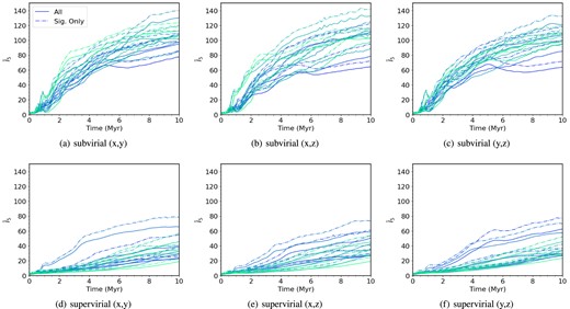
Fig. 1 shows the mean INDICATE indexes for initially substructured simulations with fractal dimension Df = 1.6 with initial radii of 1 pc. The general trend across all three lines of sight [(x, y), (x, z), and (y, z)] for the subvirial regions (top row, panels a–c) is a rapid increase in the mean INDICATE index within the first 2 Myr, and then a gradual increase in the clustering for the remainder of the simulations.
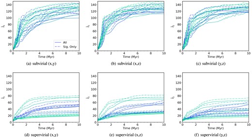
The mean INDICATE index against time for high-density, substructured, subvirial and supervirial simulations. Both the subvirial and supervirial simulations have a high initial degree of substructure (Df = 1.6) and both contain 1000 stars with initial radii of 1 pc, simulated for 10 Myr. From left to right, the columns show the INDICATE indexes calculated along three different lines of sight, (x, y), (x, z), and (y, z). The top row shows the indexes calculated for subvirial simulations, and the bottom row shows the indexes calculated for supervirial simulations. The solid lines show the mean index for all stars, and the dashed lines show the mean index for the significantly clustered stars. We show the 10 simulations we run for the different sets of initial conditions, with the colour shading of the lines being consistent across the different lines of sight.
We show how different initial conditions and perspectives affect the measured amount of clustering in simulations at 5 Myr along three different lines of sight in Figs 2 and 3. Although there is some variation depending on the line of sight, this is minimal compared to the differences between the subvirial and supervirial simulations. The supervirial simulations have a much lower degree of clustering.
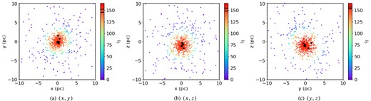
Three different line-of-sight perspectives of a subvirial simulation of 1000 stars after 5 Myr of dynamical evolution. The panels show the simulation as viewed along the z, y, and x axes. The colour of the points corresponds to their INDICATE index. The redder the points, the more clustered a star is, according to INDICATE. The 10 most massive stars are highlighted with star symbols. We show the median index for all 1000 stars with the solid black line in the colour bar (|$\tilde{I}_{5,\, \mathrm{ all}} = 146.00, 148.60, 154.00$| calculated along the z, y, and x axes, respectively), the black dashed line shows the median index for the 10 most massive stars (|$\tilde{I}_{5, 10} = 152.10, 154.20, 156.90$| calculated along the same lines of sight), and the thin black dotted line shows the significant index (Isig = 2.2); a star with an index above this is said to be significantly clustered. The scale of the colour bar is scaled based on the maximum INDICATE index found in the (y, z) plane of Imax = 158.20.
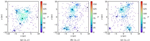
Three different line-of-sight perspectives of a supervirial simulation of 1000 stars after 5 Myr of dynamical evolution. The panels show the simulation as viewed along the z, y, and x axes. The colour of the points corresponds to their INDICATE index. The redder the points, the more clustered a star is according to INDICATE. The 10 most massive stars are highlighted with star symbols. We show the median index for all 1000 stars (|$\tilde{I}_{5,\, \mathrm{ all}} = 41.60, 27.00, 28.60$| calculated along the z, y, and x axes, respectively) with the solid black line in the colour bar, the black dashed line shows the median index for the 10 most massive stars (|$\tilde{I}_{5, 10} = 39.20, 37.00, 39.40$| calculated along the same lines of sight), and the thin dotted line shows the significant index (Isig = 2.2); a star with an index above this is said to be significantly clustered. The colour bar is scaled based on the maximum INDICATE index found in the (y, z) plane for the subvirial simulation (see Fig. 2).
The same behaviour is seen for some of the supervirial simulations (Fig. 1, panels d–f), but with a much slower initial increase in the mean indexes. The supervirial simulations also never reach the same degree of clustering according to INDICATE that the subvirial simulations do. The lower final |$\bar{I}_{5}$| in the supervirial simulations is because the stars are all initially moving away from one another. Some stars assemble themselves in small bound groupings, but the overall lower number of stars in these subgroups results in lower values of |$\bar{I}_{5}$|.
The main difference between the different initial virial states is in the final mean indexes, with subvirial simulations attaining mean indexes of ≳100 and supervirial simulations not exceeding a mean index of ∼90 by 10 Myr. This behaviour is seen across all three different lines of sight. The subvirial simulations attain higher |$\bar{I}_{5}$| due to all the stars falling into the gravitational potential well and forming a cluster (Allison et al. 2010; Parker et al. 2014), which also explains the rapid increase of |$\bar{I}_{5}$| during the first 2 Myr.
Fig. 4 shows the mean INDICATE indexes for substructured (Df = 1.6) low-density simulations with initial radii of 5 pc. We see the same general trend as in Fig. 1 with the subvirial simulations attaining higher final mean indexes (panels a–c), compared to the supervirial simulations (panels d–f). A key difference is the lack of a rapid initial increase in the clustering; due to the low density of the simulations the stars take longer to interact and so the rate of clustering is slower. We see a maximum mean index of |$\bar{I}_{5}\sim 120$| for the subvirial simulations at 10 Myr, but this is only for 1 out of the 10 simulations. The other subvirial simulations finish with |$40 \lesssim \bar{I}_{5} \lesssim 90$|, below the minimum mean index found in the much denser (|$r = 1$| pc) subvirial simulations.
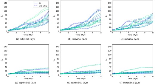
The mean INDICATE index against time for low-density, substructured, subvirial and supervirial simulations. Both the subvirial and supervirial simulations have a high initial degree of substructure (Df = 1.6) and both contain 1000 stars with initial radii of 5 pc, simulated for 10 Myr. From left to right, the columns show the INDICATE indexes calculated for three different lines of sight, (x, y), (x, z), and (y, z). The top row shows the indexes calculated for subvirial simulations, and the bottom row shows the indexes calculated for supervirial simulations. The solid lines show the mean index for all stars, and the dashed lines show the mean index for the significantly clustered stars. We show the 10 simulations we run for the different sets of initial conditions, with the colour shading of the lines being consistent across the different lines of sight.
3.2 Evolution of INDICATE in smooth regions
Fig. 5 shows the mean INDICATE indexes against time for regions with no initial substructure (Df = 3.0) and initial radii of 1 pc. When comparing between the different virial states we see similar behaviour as for subvirial and supervirial regions with Df = 1.6. We find that the final mean indexes are similar to those of the regions with Df = 1.6.
The mean INDICATE index against time for smooth, high-density, subvirial and supervirial simulations. Both the subvirial and supervirial simulations have no initial substructure (Df = 3.0) and both contain 1000 stars with initial radii of 1 pc, simulated for 10 Myr. From left to right, the columns show the INDICATE indexes calculated for three different lines of sight, (x, y), (x, z), and (y, z). The top row shows the indexes calculated for subvirial simulations, and the bottom row shows the indexes calculated for supervirial simulations. The solid lines show the mean index for all stars, and the dashed lines show the mean index for the significantly clustered stars. We show the 10 simulations we run for the different sets of initial conditions, with the colour shading of the lines being consistent across the different lines of sight.
For subvirial regions (Fig. 5, panels a–c) we see once again an initial rapid increase in the clustering before a gradual increase for the remaining duration of the simulations. The initial increase lasts longer in these simulations, with the increase lasting for around 3 Myr, compared to it finishing within 2 Myr for the substructured (Df = 1.6) simulations. We see similar behaviour for the supervirial simulations (Fig. 5, panels d–f) as well, in that they do not attain as high a mean INDICATE index by the end of the simulations.
Fig. 6 shows |$\bar{I}_{5}$| against time for low-density regions with no substructure (Df = 3.0) and initial radii of 5 pc. We see no significant difference in the evolution of the clustering between the different lines of sight. For subvirial simulations (Fig. 6, panels a–c) there is no rapid increase in |$\bar{I}_{5}$| as the stars are further apart initially, and the absence of substructure also prevents the development of clustering. This delay is substantial; there is an increase in the clustering for some of the simulations near the end of the run time, at around 7 Myr, but the majority of simulations’ INDICATE indexes do not increase. For the supervirial simulations (Fig. 6, panels d–f) the clustering does not change significantly with |$\bar{I}_{5} \lt 20$| for 10 Myr.
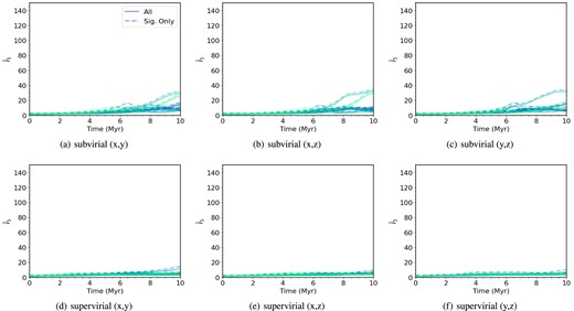
The mean INDICATE index against time for smooth, low-density, subvirial and supervirial simulations. Both the subvirial and supervirial simulations have no initial substructure (Df = 3.0) and both contain 1000 stars with initial radii of 5 pc, simulated for 10 Myr. From left to right, the columns show the INDICATE indexes calculated for different viewing angles, (x, y), (x, z), and (y, z). The top row shows the indexes calculated for subvirial simulations, and the bottom row shows the indexes calculated for supervirial simulations. The solid lines show the mean index for all stars, and the dashed lines show the mean index for the significantly clustered stars. We show the 10 simulations we run for the different sets of initial conditions, with the colour shading of the lines being consistent across the different lines of sight.
3.3 Combining methods
In this section, we present the 2D results (line of sight along the z-axis with the plane of sky being x and y) of combining the Q-parameter, ΣLDR, and ΛMSR with INDICATE. We do this for each of the simulations at the following times: 0, 1, and 5 Myr (see also Parker et al. 2014; Parker & Goodwin 2015; Blaylock-Squibbs & Parker 2023 for other examples of Q-parameter, ΣLDR, and ΛMSR being used in combination).
3.3.1 Q and INDICATE
Fig. 7 shows INDICATE plotted against Q at 0, 1, and 5 Myr in the high-density, substructured (Df = 1.6) simulations, for subvirial (panel a) and supervirial (panel b) simulations, respectively. Comparing the subvirial and supervirial simulations we see a clear distinction between them in both Q and |$\bar{I}_{5}$|. All the subvirial simulations have Q > 1 by 1 Myr, and at the same time |$\bar{I}_{5}$| lies between 20 and 100. The |$\bar{I}_{5}$| values found at 5 Myr in the subvirial simulations overlap slightly with the 1 Myr results, lying between 85 and 135.
In the high-density supervirial simulations (Fig. 7b), we find that some of the Q values at 1 and 5 Myr have remained below the boundary between substructured and smooth morphologies (stars are moving away from each other in a grouping of stars and this preserves some of the initial substructure, hence a lower Q value), with some Q values at 5 Myr overlapping with the 1 Myr values found in the subvirial simulations. The overlap between the |$\bar{I}_{5}$| values at 1 and 5 Myr has also increased, making distinguishing between the different times more difficult.

The Q-parameter plotted against INDICATE for simulations with a high degree of initial substructure (Df = 1.6). The top row shows the results for high-density simulations with initial radii of 1 pc, and the bottom row shows the results for low-density simulations with initial radii of 5 pc. The black pluses show the results at 0 Myr, the blue crosses for 1 Myr, and the red triangles for 5 Myr. The horizontal grey dash–dotted line is at 0.8, above which Q values signify the regions have a smooth, centrally concentrated morphology. The left-hand column shows the results for subvirial simulations, and the right-hand column shows the results for supervirial simulations.
Panels (c) and (d) of Fig. 7 show the results for the low-density, initially substructured (Df = 1.6) simulations. The INDICATE results for 0 and 1 Myr are similar when comparing the subvirial and supervirial realisations, due to a lack of dynamical evolution at early times. We once again see that the 5 Myr Q values are higher in the subvirial regions as the substructure is more effectively erased due to the stars collapsing inwards into the gravitational potential well. On the other hand, the supervirial regions retain substructure, but do not become more clustered due to a lack of significant dynamical evolution.
Fig. 8 shows the Q and |$\bar{I}_{5}$| values for initially smooth subvirial (left-hand panels) and supervirial (right-hand panels) simulations, respectively. Panels (a) and (b) show simulations that are high density with Df = 3.0 (little to no initial degree of substructure). For subvirial simulations (panel a) both Q and |$\bar{I}_{5}$| values are distinct with very little overlap between the different times. For the supervirial simulations (panel b) there is much more overlap, with Q values being similar across 0, 1, and 5 Myr, and only the INDICATE values increase slightly over time. As in the highly substructured simulations, we find that the maximum |$\bar{I}_{5}$| values are found in the subvirial simulations.
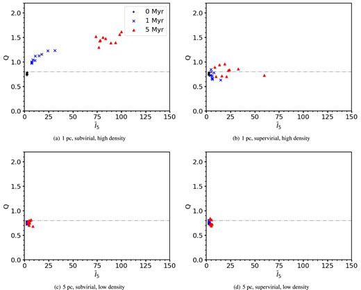
The Q-parameter plotted against INDICATE for simulations with little to no initial substructure (Df = 3.0). The top row shows the results for high-density simulations with initial radii of 1 pc, and the bottom row shows the results for low-density simulations with initial radii of 5 pc. The black pluses show the results at 0 Myr, the blue crosses for 1 Myr, and the red triangles for 5 Myr. The horizontal grey dash–dotted line is at 0.8, above which Q values signify the regions have a smooth, centrally concentrated morphology. The left-hand column shows the results for subvirial simulations, and the right-hand column shows the results for supervirial simulations. The top row shows the high-density simulations, and the bottom row shows the low-density simulations.
In panels (c) and (d) of Fig. 8, we show the evolution of non-substructured (Df = 3.0), low-density (r = 5 pc) simulations and we find the Q values overlap across 0, 1, and 5 Myr. This overlap is seen for both subvirial and supervirial simulations implying that the initial virial state of low-density regions without substructure cannot be constrained using these methods.
3.3.2 ΣLDR and INDICATE
Parker et al. (2014) and Parker (2014) show that the relative surface densities of the most massive stars can be used in tandem with the Q-parameter to infer the initial density and virial state of a star-forming region.
Figs 9(a) and (b) show the results for ΣLDR and INDICATE for high-density and highly substructured regions with Df = 1.6. The ΣLDR values are less reliable at inferring the initial conditions than the Q values, with an overlap between ΣLDR between the subvirial and supervirial simulations at 1 and 5 Myr. The |$\bar{I}_{5}$| values are the same here so the analysis in the previous section will apply for the rest of this section.
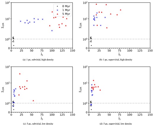
The relative surface density of massive stars, ΣLDR, plotted against INDICATE for simulations with a high degree of initial substructure (Df = 1.6). The black pluses show the results for 0 Myr, the blue crosses for 1 Myr, and the red triangles for 5 Myr. The horizontal grey dash–dotted line is at 1, above which ΣLDR finds the 10 most massive stars are in areas of greater than average surface density. The top row shows the results for high-density simulations with initial radii of 1 pc, and the bottom row shows the results for low-density simulations with initial radii of 5 pc. The left-hand column shows the results for subvirial simulations, and the right-hand column shows the results for the supervirial simulations.
Panels (c) and (d) show the combination for low-density simulations. Comparing across the subvirial and supervirial simulations we see some overlap in the ΣLDR values for the 0 and 1 Myr snapshots, although after 5 Myr it is possible to distinguish between the high- and low-density simulations.
Figs 10(a) and (b) show the results for dense simulations with no initial substructure (Df = 3.0). The dense, subvirial simulations (panel a) show a very distinct difference between 1 and 5 Myr (compared the triangles with the crosses), but the distinction is less clear for the supervirial simulations (ostensibly because the degree of clustering measured by INDICATE does not increase as much in the supervirial simulations).
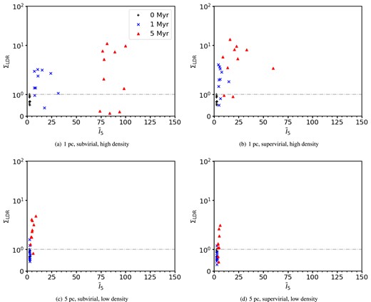
The relative surface density of massive stars, ΣLDR, plotted against INDICATE for simulations with no initial substructure (Df = 3.0). The black pluses show the results for 0 Myr, the blue crosses for 1 Myr, and the red triangles for 5 Myr. The horizontal grey dash–dotted line is at 1, above which ΣLDR finds the 10 most massive stars are in areas of greater than average surface density. The top row shows the results for high-density simulations with initial radii of 1 pc, and the bottom row shows the results for low-density simulations with initial radii of 5 pc. The left-hand column shows the results for subvirial simulations, and the right-hand column shows the results for the supervirial simulations.
In the low-density simulations without substructure (panels c and d of Fig. 10) there is a significant overlap of ΣLDR versus |$\bar{I}_{5}$| at all snapshot times, and as such it is impossible to differentiate between initially subvirial and supervirial simulations.
We find that in the substructured simulations ΣLDR values tend to be higher at 5 Myr compared to simulations with no substructure, and the degree of clustering measured by INDICATE is also slightly higher in the substructured simulations.
3.3.3 ΛMSR and INDICATE
In addition to plotting the evolution of the Q-parameter against the relative surface density ratio, ΣLDR, Parker et al. (2014) showed that it is possible to also distinguish between subvirial and supervirial initial conditions by using a combination of Q and the mass segregation ratio, ΛMSR.
Fig. 11 shows the combination of ΛMSR and INDICATE for initially substructured simulations (Df = 1.6). Although subvirial simulations tend to attain higher ΛMSR values (Allison et al. 2010; Parker et al. 2014), not all simulations dynamically segregate. This combined with the widespread in INDICATE indexes makes inferring the initial virial state of dense regions using ΛMSR and INDICATE alone unreliable (compare panels a and b). The ΛMSR values are also similar between the subvirial and supervirial simulations in the low-density initial conditions (panels c and d). The key difference between the low- and high-density simulations is the ΛMSR values at 1 Myr tending to be higher in the subvirial high-density simulations compared to the supervirial high-density simu-lations.
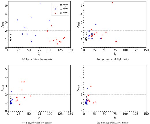
ΛMSR versus INDICATE for simulations with a high degree of initial substructure (Df = 1.6). The black pluses show the results for 0 Myr, the blue crosses for 1 Myr, and the red triangles for 5 Myr. The grey dash–dotted line is at ΛMSR = 2, above this the 10 most massive stars are mass segregated. The top row shows the results for high-density simulations with initial radii of 1 pc, and the bottom row shows the results for low-density simulations with initial radii of 5 pc. The left-hand column shows the results for subvirial simulations, and the right-hand column shows results for supervirial simulations.
Fig. 12 shows the results for simulations with no initial substructure (Df = 3.0). Comparing the high-density simulations we see no significant difference in the ΛMSR values, with a single simulation in both sets attaining ΛMSR > 4, which is a significant degree of mass segregation.
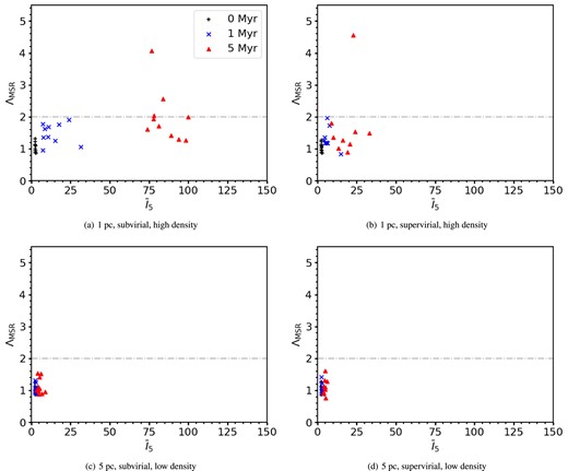
ΛMSR versus INDICATE for simulations with no initial substructure (Df = 3.0). The black pluses show the results for 0 Myr, the blue crosses for 1 Myr, and the red triangles for 5 Myr. The grey dash–dotted line is at ΛMSR = 2, above this the 10 most massive stars are mass segregated. The top row shows the results for high-density simulations with initial radii of 1 pc, and the bottom row shows the results for low-density simulations with initial radii of 5 pc. The left-hand column shows the results for subvirial simulations, and the right-hand column shows the results for supervirial simulations.
However, the combination of ΛMSR and INDICATE does provide some constraints, the smooth, subvirial simulations (panel a) are distinguishable from the supervirial simulations (panel b).
For the low-density simulations (panels c and d) the two different initial virial states are indistinguishable.
3.4 Determining the initial degree of substructure
We have shown that combining INDICATE with other measures of the spatial distribution of stars can be used to infer the initial density of a star-forming region, and whether the star-forming region was initially subvirial or supervirial.
Observations suggest that many star-forming regions form with the stars arranged in a substructured distribution, likely to be inherited from the filamentary nature of the gas from which they form. The substructure is not created during the dynamical evolution of a star-forming region, it is always erased (Goodwin & Whitworth 2004; Parker et al. 2014; Daffern-Powell & Parker 2020).
Hydrodynamical simulations of the early phases of star formation suggest that the initial degree of substructure of stars can vary quite considerably (Schmeja & Klessen 2006; Dale et al. 2012, 2013, 2014; Girichidis et al. 2012). As any observed star-forming region could have experienced some dynamical evolution, it is not clear what the typical degree of substructure is for star-forming regions (or even if there is a typical value).
Furthermore, Dib & Henning (2019) suggest that the value of the Q-parameter increases with increasing star formation rate, and postulate a link between the early stages of star formation in clouds, and the later degree of substructure. This could, however, be affected by any later dynamical evolution of the stars (Parker et al. 2014; Parker & Dale 2017), and if there is not a direct mapping of the structure of the gas to the stars (Parker & Dale 2015).
Inspection of our results suggests that combining INDICATE with other measures of the spatial (and kinematic) information could be used to infer the initial degree of substructure. The most important factor in determining the amount of dynamical evolution is the initial local density within the star-forming region (Parker 2014). This means that in order to compare the effects of the substructure on the evolution of a star-forming region, we must compare regions with similar median local densities.
For regions with similar radii, a highly substructured region (Df = 1.6) will have a very high median density compared to a region with no substructure (Df = 3.0). Our substructured regions with large radii (5 pc) have similar median local densities (|$\tilde{\rho } \sim 100$| M⊙ pc−3) to our smooth regions (Df = 3.0) with smaller radii (1 pc), and so we determine the effects of substructure on the evolution of INDICATE using these pairs of simulations.
As an example, we compare the evolution of the Q-parameter and INDICATE for substructured simulations with large radii (Fig. 7c) to smooth simulations with more compact radii (Fig. 8a). We can see that both Q and INDICATE display a higher level of clustering in the more compact, smoother simulations, and this is also evident in the subsequent plots that show the evolution of INDICATE combined with ΛMSR (compare Fig. 11c to Fig. 12a) or ΣLDR (compare Fig. 9c to Fig. 10a).
This is interesting because for most combinations of metrics, their signal is enhanced from the dynamical evolution of initially substructured regions. Because the degree of clustering measured by INDICATE is highest for smooth rather than substructured regions (of comparable median local densities), INDICATE can be used in tandem with other metrics to distinguish between subtle differences in the initial degree of substructure in star-forming regions.
4 CONCLUSIONS
We apply the INDICATE clustering measure (Buckner et al. 2019) to eight sets of N-body simulations consisting of 1000 stars along three different lines of sight to understand how it behaves due to dynamical evolution in star-forming regions with different initial conditions. We also combine INDICATE with other methods to assess its diagnostic ability in determining the initial conditions of the simulations from later snapshots. Our conclusions are as follows.
INDICATE is not significantly affected by projection effects in our simulations, and evolves similarly when measured along different lines of sight for the same set of simulations.
INDICATE does evolve differently depending on the initial virial state of the simulations. We find that |$\bar{I}_5$| increases rapidly in the subvirial simulations during the first 2 Myr, and then steadily increases until the end of the simulations. This behaviour is seen in both simulations with a high degree of initial substructure (Df = 1.6) and in simulations with no initial substructure (Df = 3.0), albeit to a lesser extent in the less substructured simulations.
The values of the INDICATE measure, |$\bar{I}_{5}$|, are higher for subvirial simulations than for supervirial simulations at the end of the simulations (10 Myr), and this is seen in all sets of simulations apart from very low density, initially non-substructured Df = 3.0 simulations, where there has been little to no dynamical evolution.
INDICATE is most sensitive to the initial density, rather than the initial degree of substructure in a region. The higher the initial density of a star-forming region, the more clustered the stars tend to become.
However, INDICATE – in combination with other metrics such as the Q-parameter – can be used to infer the initial degree of substructure, but only if the initial densities and virial ratios are known. For example, compare Figs 7 and 8, where the plot of Q versus |$\bar{I}_{5}$| gives different results for high-density simulations with and without substructure. This difference is much less pronounced for the low-density simulations.
When we combine INDICATE with other measures of spatial clustering, we find that INDICATE used in combination with the Q-parameter (Cartwright & Whitworth 2004) provides the most reliable way of inferring the initial conditions of the simulated star-forming regions.
Ideally, combinations of more than one spatial diagnostic (e.g. INDICATE and Q, Q and ΣLDR, etc.) are required to really pinpoint the initial conditions of a star-forming region, in addition to kinematic measures such as the distributions of ejected stars (Schoettler et al. 2019, 2020; Farias, Tan & Eyer 2020; Parker & Schoettler 2022; Schoettler, Parker & de Bruijne 2022; Arunima, Pfalzner & Govind 2023).
ACKNOWLEDGEMENTS
The plots in this paper have been created using matplotlib 3.3.4 (Hunter 2007). Numerical results have been calculated using numpy and scipy 1.9.0 (Harris et al. 2020; Virtanen et al. 2020).
GABS acknowledges support from the University of Sheffield in the form of a publication scholarship and the University of Sheffield Institutional Open Acess Fund. RJP acknowledges support from the Royal Society in the form of a Dorothy Hodgkin Fellowship.
For the purpose of open access, the author has applied a Creative Commons Attribution (CC BY) license to any author accepted manuscript version arising from this submission.
DATA AVAILABILITY
The simulation data used in this paper are available publicly on the ORDA data repository. Subvirial simulation set: https://orda.shef.ac.uk/articles/dataset/Subvirial_Simulations/25205207. Supervirial simulation set: https://orda.shef.ac.uk/articles/dataset/Supervirial_Simulations/25205846.
Footnotes
In this paper, we use the term ‘star-forming region’ to refer to a population of young stars that we assume formed from the same giant molecular cloud. This star-forming region may be gravitationally bound, in which case it would be classified as a cluster, or unbound, in which case it would be an association. As we model the evolution of both bound and unbound stellar populations in this paper, we use ‘star-forming region’, though some researchers exclusively reserve this term for populations of stars still surrounded by gas left over from the star formation process.
References
Author notes
Royal Society Dorothy Hodgkin fellow.
