


ABSTRACT
A new CO|$^+$| fluorescence emission model for analysing cometary spectra is presented herein. Accurate line lists are produced using the PGOPHER software for all transitions between the three electronic states (X |$^2\Sigma$|, A |$^2\Pi$|, B |$^2\Sigma$|) with vibrational states up to |$v_\textrm {max} = 9, 8, 6$|, respectively, and maximum rotational states with rotational quantum numbers |$N\le 20$|. As a result of improved molecular constants and theoretical transition rates, an expansion of the utilized solar spectrum into the infrared, and the substantial expansion of the included rovibronic states, the model provides an update of the fluorescence efficiencies of the CO|$^+$| cation. The dependencies on heliocentric velocity and distance are explicitly included. We report, for the first time, quantification of the fluorescence efficiencies for the ground state rovibrational transitions of CO|$^+$| and predict the positions and relative intensities of CO|$^+$| lines in windows accessible to both ground- and space-based observatories. The computed fluorescence efficiencies show excellent agreement with UV/optical observations of both C/2016 R2 (PanSTARRS) and 29P/Schwassmann-Wachmann 1. The updated fluorescence efficiencies allow for revised N|$_2$|/CO abundances for comets 1P/Halley, C/1987 P1 (Bradfield), and C/2016 R2 (PanSTARRS), which can change by up to 30 per cent when accounting for recent improvements to CO|$^+$| and N|$_2^+$| fluorescence efficiencies. The model code, input files, and fluorescence efficiencies are publicly available and distributed on permanent archives for future uses in cometary analyses.
1 INTRODUCTION
Comets are relatively unprocessed remnants leftover from the era of planet formation. As comets approach the sun, their volatile contents sublimate and undergo photochemistry. These volatiles, along with their fragment species produced from photochemistry or collisions, fluoresce and emit across the ultraviolet, visible, and infrared regimes. Remote spectroscopic observations of these emissions provide unique diagnostics of cometary comae compositions, from which properties of the nucleus and evolutionary history can sometimes be inferred. However, many of the emission lines in high-resolution comet spectra remain unidentified, owing in part either to missing spectroscopic data or fluorescence models used to predict relative line heights, so-called ‘fluorescence efficiencies’ (g-factors). A ready example is available in the high-resolution spectrum of Comet 122P/de Vico, in which over 4000 lines remain unidentified (Cochran & Cochran 2002). Even in low-resolution observations, fluorescence models may be insufficient for identifying the present species and their photochemical complexities.
The most abundant volatiles in the coma, mainly H|$_2$|O and to a lesser extent CO and CO|$_2$|, can give rise to several cations, including H|$_2$|O|$^+$|, CO|$^+$|, and CO|$_2^+$| (Fortenberry, Bodewits & Pierce 2021). The presence of CO|$^+$| around comets has long been known, and its emission has been identified around comets as far back as 1909 (Fowler 1909) by comparison to spectra acquired in the laboratory. The aptly named ‘Comet-Tail Bands’ were later confirmed by observations of CO|$^+$| emissions in the tails of multiple comets (Swings 1965). However, observations of CO|$^+$| in comets can be limited by several (or many) compounding factors, including a low precursor abundance (e.g. CO), acceleration of CO|$^+$| by the solar wind into the tail, observing geometry, telluric contamination, and possibly multiple production mechanisms. In some cases, the simultaneous observations of CO|$^+$| and N|$_2^+$| emission have enabled some constraints on the N|$_2$|/CO abundance ratio, which provides insights into the formation regions of these comets. For example, Lutz, Womack & Wagner (1993) observed the ion tails of comets 1P/Halley and C/1987 P1 (Bradfield) in order to derive constraints on the ionic abundances. Optical studies of 29P/Schwassmann-Wachmann 1 revealed emission features from both CO|$^+$| and N|$^+_2$| which were used to constrain the N|$_2$|/CO abundance ratio (Ivanova et al. 2016). Most recently, observations of the rare CO- and N|$_2$|-rich comet C/2016 R2 (PanSTARRS) showed substantial emission from CO|$^+$| and N|$^+_2$|, allowing for some investigations of the N|$_2$|/CO abundance (Cochran & McKay 2018; Opitom et al. 2019; Anderson et al. 2022).
The likely precursor of CO|$^+$|, CO, sublimates readily beyond several AU where water sublimation becomes increasingly inefficient (Womack, Sarid & Wierzchos 2017), and the neutral CO distribution may be caused by one or more production mechanism(s) (Pierce & A’Hearn 2010). Once produced, CO|$^+$| may serve as a proxy for CO in such distant comets if the emission and production mechanisms can be characterized (Fortenberry, Bodewits & Pierce 2021). However, this presents several difficulties. While the frequencies of the ground state vibrational bands of CO|$^+$| lie in favourable windows for both ground- and space-based observatories, their fluorescence efficiencies have never been characterized. Even in spectral windows favourable to ground-based facilities, e.g. the near-ultraviolet and optical regimes, many of these analyses have relied on the band luminosities of CO|$^+$| reported in Magnani & A’Hearn (1986), which are in some ways incomplete. In the intervening years since the publication of Magnani & A’Hearn (1986), experimental and theoretical pursuits have greatly improved the spectroscopic parameters of CO|$^+$|, and computational resources are capable of solving the relevant differential equations for large systems of energy levels. Furthermore, Magnani & A’Hearn (1986) provide band luminosities on a grid of heliocentric velocities, but transition-specific g-factors that are useful for interpreting e.g. high-resolution UV/optical comet spectra of the CO|$^+$| emission in C/2016 R2 (Cochran & McKay 2018; Opitom et al. 2019), are not available. While the model of Magnani & A’Hearn (1986) is described in print, the source code of their model is no longer available.
The current study builds upon the fluorescence code previously introduced by Bromley et al. (2021) to develop an updated model for CO|$^+$| fluorescence. The new model enables a comprehensive analysis of CO-driven activity and emission, spanning from ultraviolet to infrared wavelengths. First, we construct an accurate line list of CO|$^+$| for use in this model from molecular constants compiled from recent high-resolution experimental studies of CO|$^+$| emission in conjunction with the PGOPHER program (Western 2017). We pursue fluorescence efficiency calculations for the band systems of CO|$^+$|, and investigate the heliocentric velocity, distance, and time dependencies of the fluorescence emission. Lastly, the model is tested against cometary observations of CO|$^+$|. The model code, input files, and associated data required to run the model are distributed on GitHub,1 through the Zenodo service,2 and uploaded to the NASA Planetary Data System.3
2 FLUORESCENCE MODELLING
2.1 Fluorescence in equilibrium
The computation of fluorescence efficiencies, also known as ‘g-factors’, proceeds as follows. For a given energy level i, population is sourced from (1) radiative decay(s) from level(s) j, characterized by the transition rate (Einstein A coefficient) |$A_{j\rightarrow {i}}$|; (2) absorption from lower (in energy) levels indexed by k into level i with rate |${\rho }B_{k\rightarrow {i}}$| where B is an Einstein coefficient, |$\rho$| is the radiation field (in compatible units); and (3) stimulated emission described by the rate |${\rho }B_{i\rightarrow {j}}$|, which is typically negligible (Bromley et al. 2021).
The system of equations describing the N level populations is written for each level i as
which results in N coupled equations and |$N-1$| unknowns. When fluorescence equilibrium is assumed, |$dn/dt = 0$| and one equation is replaced by the normalization condition |$\sum _i n_i = 1$| (Magnani & A’Hearn 1986; Bromley et al. 2021). Alternatively, one can solve for level populations with respect to the ground state, and a modified normalization condition yields the same effective solution (Manfroid, Hutsemékers & Jehin 2021). Regardless of normalization condition, the equilibrium (fractional) level populations |${\bf x}$| are found by effectively solving equation (1), which can be cast into the matrix form |$A{\bf x} = B$|, where the rates for all populating and depopulating processes are stored in matrix A. This approach is ubiquitous in calculations of both molecular and atomic g-factors (see e.g. Magnani & A’Hearn 1986), which follow as (in units of J s|$^{-1}$| mol.|$^{-1}$|)
where |$hc/\lambda _{ji}$| is the photon energy of the transition, |$n_j$| is the equilibrium population of the upper level involved in the transition, and |$A_{j\rightarrow {i}}$| is the transition rate.
In the above description, the line (absorption) profile |$\phi (\lambda)$| can be assumed to be sufficiently small such that |$\int \rho \phi (\lambda)d\lambda = \rho (\lambda _{ji})$| and the absorption rate follows as simply |${\rho (\lambda _{ji})}B_{ij}$|. One can alternatively assume a thermal (Doppler) line profile, and numerical integration over the radiation field yields the appropriate absorption rate. We utilize here a delta function line profile.
The balance between absorption and spontaneous emission is sensitive to the intensity of the incident solar radiation. We utilize the same solar spectrum provided by Bromley et al. (2021), which is compiled from multiple observations and theoretical sources. The bulk of the solar spectrum is sourced from Coddington et al. (2021), who combined multiple measurements of the solar spectrum to produce a flux atlas spanning 202–2730 nm. For this work, we expanded this solar spectrum to 14 μm using the Planetary Spectrum Generator (PSG; Villanueva et al. 2018). Using the PSG, we generated an infrared solar spectrum with resolving power |$R = 200\, 000$|. The infrared PSG spectrum is joined to the Bromley et al. (2021) spectrum by applying a minor scaling factor (|$\sim 5~{{\ \rm per\ cent}}$|) to the PSG spectrum in order to join their continua at |$\sim 2 \,\mu$|m. Transitions redward of 14 μm are included in our models for the purposes of determining level populations, but are not pumped by any radiation field.
2.2 Time-dependent fluorescence
In certain situations, it might be more suitable to compute the level populations and g-factors in a time-dependent manner. This approach allows for a more accurate representation of dynamic processes, as it takes into account the temporal evolution of these quantities. One can imagine such cases occurring in the inner coma where photochemical lifetimes may be small, and thus nucleus-centered comet observations with a small field of view may be sampling a population that has not achieved fluorescence equilibrium. In the time domain, the system of equations describing the fractional level populations |$\vec{x}(t)$| becomes:
whose solution can be written as
Assuming A is a diagonalizable matrix, equation (4) can be recast into matrix form (LeVeque 2007) as
where matrix P contains the (column) eigenvectors of matrix A, |$P^{-1}$| is the matrix inverse of P, and matrix D is written as
where |$\lambda _i$| is the |$i^{\it th}$| eigenvalue of the original matrix A and all off-diagonal elements are 0. Thus, the solution at time |$t_f$| is propagated directly from time |$t=0$| to time |$t_f$| using only the eigenvalues and eigenvectors of the rate matrix A. In practice, the matrix exponential method offers a convenient choice of the initial level populations in the user-defined variable |$\vec{x}(t=0)$|. This convenience allows for the computation of time-dependent g-factors for either single or many initial population channels and may be of use in exploring emission from channels initially populated by e.g. collisional effects.
In the time domain, the expression for the g-factor (equation 2) must be modified to account for the time-evolution of the level populations. The instantaneous g-factor at time t is simply:
where |$n_j(t)$| is the time-dependent population computed from equation (5). An alternative quantity of interest is the time-dependent g-factor observed from time |$t = 0$| to time |$t_f$|, i.e. the time-integrated g-factor:
where |$dn_j/dt$| can be numerically evaluated from the time-dependent populations computed with equation (5). In analysing comet spectra with species that are not in fluorescence equilibrium, the latter form of the time-dependent g-factor is likely most appropriate. However, application of this formalism also necessitates the inclusion of a density-dependent model that includes quantification of the photochemical lifetimes. Such an application is beyond the scope of this work, but preliminary investigations of time-dependent effects in CO|$^+$| fluorescence are discussed in Section 4.2.
The above methods have been implemented in a modified version of the Python code ‘FlorPy’ described in Bromley et al. (2021). The present authors have made the modified (time-dependent) code and utility codes relevant to the present manuscript publicly available via GitHub. In the course of this work, we have also made several improvements to the code, including an improved handling of variably spaced wavelength grids in solar spectra, significantly faster integration routines, and a non-negative least-squares matrix solver that enables calculations out to very large heliocentric distances. These changes result in a |$\sim$|30-fold increase in speed which allow calculations involving large time grids or numbers of transitions to be tractable on modern personal computers.
2.3 Constructing a molecular fluorescence model
To produce the necessary inputs for the fluorescence model calculations, we utilize the PGOPHER software (Western 2017), which is widely used in the molecular physics community to analyse high-resolution emission or absorption spectra of molecular species, such as the recent analyses of e.g. ZrO (Sorensen & Bernath 2021) or CaH (Li et al. 2012). In the present work, PGOPHER was instead utilized with a standard (|$\hat{N}^2$|) effective Hamiltonian (see discussion in Western 2017) to produce rovibronically resolved line and energy level lists of CO|$^+$| from existing constants in the literature. PGOPHER outputs are then converted from their native format into line and energy level lists similar in structure to those utilized by the National Institute of Standards and Technology (NIST) Atomic Spectra Database (ASD; Kramida et al. 2023) for atomic systems. In doing so, we allow for import without modification into the machinery of the fluorescence model.
The methods described below are also applicable for any diatomic species, provided the requisite molecular constants and transition rates are available. In instances where experimental data does not adequately characterize the rovibronic level structure or is otherwise unavailable, quantum chemical calculations can offer valuable insights that facilitate identification in astrophysical observations, or can guide future experimental efforts. For example, recent quantum chemical calculations for CO|$^+$|, H|$_2$|O|$^+$|, and H|$_2$|CO|$^+$| by Davis, Huang & Fortenberry (2023a) and Davis, Garrett & Fortenberry (2023b) have shown remarkable agreement with energies and constants derived from experiments and may provide insights for other species which present considerable difficulties in the laboratory.
All present CO|$^+$| models include three electronic states: the ground electronic state, X |$^2\Sigma$|, the first electronic excited state A |$^2\Pi$|, and the second electronic state B |$^2\Sigma$|. Within each electronic state, the vibrational levels denoted by quantum number v have rotational levels denoted by the quantum number N. In the two |$\Sigma$| states that have total orbital angular momentum |$\Lambda = 0$|, the |$N \ne 0$| levels are doubly degenerate in the absence of spin. The coupling between spin (|$\Sigma = \pm 1/2$|) and molecular rotation lifts the degeneracy of the two levels, which are denoted by their total angular momentum |$J = N \pm 1/2$|. In the two |$\Sigma$| states, the energy difference between the two J levels of each N rotational state is small (|$\lt 0.01$| cm|$^{-1}$|).
In the A |$^2\Pi$| state, the coupling between the total orbital angular momentum (|$|\Lambda | = 1$|) and spin (|$\Sigma = \pm 1/2$|), yields two branches denoted by the quantum number |$\Omega = \Lambda + \Sigma$|. The two branches, A |$^2\Pi _{\Omega = 1/2}$| and A |$^2\Pi _{\Omega = 3/2}$|, are well separated in energy and are inverted, i.e. the energy of the |$\Omega = 1/2$| component is higher than the |$\Omega = 3/2$| component. Each rotational level denoted by N is split into a spin doublet labelled by the total angular momenta |$J = N \pm 1/2$|, with each J level doubly degenerate due to the two possible projections of the total orbital angular momentum on to the molecular axis (|$\Lambda = \pm 1$|), resulting in two degenerate spin components. This degeneracy is referred to as ‘|$\Lambda$|-type’ doubling. The degeneracy of the |$\Lambda$|-doubled levels is broken by interactions with other electronic states, resulting in a small energy splitting between the two |$\Lambda$|-resolved components of each J level.
The interactions described above are characterized by standardized molecular constants (see e.g. Hirota et al. 1994) which are used as inputs to the PGOPHER calculations (Western 2017). The molecular constants used in our PGOPHER calculations are summarized in Table 1, which we discuss briefly. For the two |$\Sigma$| states, we included the following interactions with their associated constant labels in parentheses: molecular rotation (B), centrifugal distortion constant (D), and spin–rotation coupling (|$\gamma$|). In the first electronically excited state, A |$^2\Pi$|, the required molecular constants include the aforementioned rotation and centrifugal distortion, spin–orbit coupling (A), and its associated distortion term (|$A_D$|). Within each J state, the energy splitting resulting from |$\Lambda$|-type doubling is parametrized by the molecular constants p and q. While the effects of spin–rotation coupling for |$\Sigma$| states and |$\Lambda$|-type doubling for A |$^2\Pi$| result in minor changes in the transition wavelengths, the effects are included to ensure that the wavelengths in the final line lists are not degenerate. This greatly simplifies the import of the lines and levels into the machinery of the fluorescence code, as transitions are internally matched to their corresponding levels by the level energies and J values associated with the transitions.
Compiled molecular constants and vibrational energies of the X |$^2\Sigma$|, B |$^2\Sigma$|, and A |$^2\Pi$| states of CO|$^+$|. Vibrational energies |$(E)$| with respect to X |$^2\Sigma$| (|$v=0$|), rotational constant (B), centrifugal distortion constant (D), spin-rotation coupling (|$\gamma$|), spin-orbit coupling (A), centrifugal distortion of spin-orbit coupling (|$A_D$|), and |$\Lambda$|-type doubling parameters q and p are reported in units of cm|$^{-1}$|. The sources of each constant and term energy are given by the reference above each quantity with labels S2004 (Szajna, Kepa & Zachwieja 2004), K2004 (Kepa et al. 2004), and C1982 (Coxon & Foster 1982). Powers of 10 are indicated by the letter ‘E’ and following numbers, e.g. E-6 = 10|$^{-6}$|.
| Constant | |$v = 0$| | |$v = 1$| | |$v = 2$| | |$v = 3$| | |$v = 4$| | |$v = 5$| | |$v = 6$| | |$v = 7$| | |$v = 8$| | |$v = 9$| |
|---|---|---|---|---|---|---|---|---|---|---|
| X |$^2\Sigma$| | ||||||||||
| Source | S2004 | S2004 | S2004 | S2004 | S2004 | S2004 | S2004 | S2004 | S2004 | S2004 |
| E | 0 | 2183.9129 | 4337.5041 | 6460.7604 | 8553.6684 | 10616.215 | 12648.3869 | 14650.1708 | 16621.5534 | 18562.5215 |
| B | 1.967459 | 1.948449 | 1.929399 | 1.91024 | 1.890945 | 1.871708 | 1.852381 | 1.833008 | 1.813645 | 1.79361 |
| D | 6.317E-06 | 6.346E-06 | 6.371E-06 | 6.424E-06 | 6.39E-06 | 6.45E-06 | 6.433E-06 | 6.515E-06 | 6.647E-06 | 5.95E-06 |
| |$\gamma$| | 9.105E-03 | 9.045E-03 | 8.965E-03 | 8.862E-03 | 8.734E-03 | 8.582E-03 | 8.406E-03 | 8.20E-03 | 7.982E-03 | 7.734E-03 |
| B |$^2\Sigma$| | ||||||||||
| Source | S2004 | S2004 | S2004 | S2004 | S2004 | S2004 | S2004 | |||
| E | 45632.5334 | 47311.8995 | 48938.2774 | 50514.038 | 52041.5515 | 53523.1888 | 54961.3203 | |||
| B | 1.784661 | 1.754589 | 1.724232 | 1.693906 | 1.663777 | 1.634137 | 1.6069 | |||
| D | 7.975E-06 | 8.15E-06 | 8.422E-06 | 8.608E-06 | 8.717E-06 | 8.929E-06 | 9.181E-06 | |||
| |$\gamma$| | 2.1339E-02 | 2.065E-02 | 1.936E-02 | 1.824E-02 | 1.843E-02 | 1.815E-02 | 1.534E-02 | |||
| A |$^2\Pi$| | ||||||||||
| Source | K2004 | K2004 | K2004 | K2004 | K2004 | C1982 | K2004 | K2004 | K2004 | |
| E | 20406.17246 | 21941.04957 | 23449.04753 | 24930.21824 | 26384.61361 | 27812.28552 | 29213.28588 | 30587.66659 | 31935.47956 | |
| B | 1.579557 | 1.560171 | 1.5407359 | 1.521297 | 1.501899 | 1.48285 | 1.463182 | 1.443841 | 1.42367 | |
| D | 6.61E-06 | 6.67E-06 | 6.631E-06 | 6.612E-06 | 6.544E-06 | 6.85E-06 | 6.737E-06 | 6.882E-06 | 6.23E-06 | |
| A | |$-$|122.0582 | |$-$|121.98047 | |$-$|121.8944 | |$-$|121.8323 | |$-$|121.8745 | |$-$|121.35 | |$-$|120.3656 | |$-$|120.4136 | |$-$|120.413 | |
| |$A_D$| | |$-$|1.764E-04 | |$-$|1.585E-04 | |$-$|1.391E-04 | |$-$|1.241E-04 | |$-$|1.13E-04 | N/A | |$-$|6.31E-04 | |$-$|2.76E-04 | |$-$|6.00E-05 | |
| q | |$-$|2.216E-04 | |$-$|2.21E-04 | |$-$|2.395E-04 | |$-$|2.21E-04 | |$-$|2.22E-04 | |$-$|2.47E-04 | |$-$|7.50E-05 | |$-$|9.01E-04 | |$-$|1.67E-03 | |
| p | 1.387E-02 | 1.302E-02 | 1.2344E-02 | 1.071E-02 | 7.85E-03 | 1.60E-02 | 2.532E-02 | 7.21E-03 | 1.10E-03 |
The molecular constants are sourced from the most-complete experimental analyses available. For the |$v = 0 - 9$| terms of the ground state (X |$^2\Sigma$|) and the |$v = 0 - 6$| terms of B |$^2\Sigma$|, the term energies, band origins, and rotational constants are taken from Szajna, Kepa & Zachwieja (2004). The vibrational energies and rotational constants for the |$v = 0 - 4$| and |$v = 6 - 8$| terms of A |$^2\Pi$| are taken from Kepa et al. (2004). The |$v = 5$| term is absent from the analysis of Kepa et al. (2004), as some rotational levels of the A |$^2\Pi ~(v = 5)$| term are known to be perturbed by the |$v = 14$| term of X |$^2\Sigma$| by as much as 14 cm|$^{-1}$| (Coxon & Foster 1982). We include the |$v = 5$| term with the constants from Coxon & Foster (1982) with the understanding that some line positions may be inaccurate for select transitions involving the A |$^2\Pi (v=5$|) levels.
In our compilation of the molecular constants, the band origins (energies) of the B |$^2\Sigma$| and A |$^2\Pi$| levels are calculated separately using the constants reported in Szajna, Kepa & Zachwieja (2004) and Kepa et al. (2004). In the present calculations, the energies of the two excited states are independently shifted such that the ground level of X|$~^2\Sigma$| is set to zero. The largest errors introduced in the computed wavenumbers are thus in the Baldet–Johnson (B|$~^2\Sigma$|–A|$~^2\Pi$|) system as the constants were not extracted from a simultaneous fit of all three considered band systems. The Baldet–Johnson band emission is produced by radiative decays of B |$^2\Sigma$| vibrational levels into those in A |$^2\Pi$|, where the energies and exciting solar spectrum for the former are accurate, and pumping between the two excited states can be ignored. As the Baldet–Johnson system is very weak in fluorescence and the wavelength errors introduced by these choices are small compared to the wavelength resolution of most if not all cometary spectra, the effect on the computed g-factors is negligible.
For rovibronic transitions, the transition rate is generally separated into the product of three components, i.e. electronic, vibrational, and rotational components. With regards to the electronic component, the transition dipole moment, |$R_e^2$|, can be calculated from the electronic and vibrational wave functions. The vibrational component, the Franck–Condon factor |$| \langle v^{\prime } | v^{\prime \prime } \rangle |^2$|, can be computed from the same vibrational wave functions, which themselves are computed ab initio or by using semi-empirical methods utilizing standard molecular constants (Qin, Zhao & Liu 2017). The distribution of the band transition rate among the various rotational components is captured in the Hönl–London factors, which are computed from the rotational wave functions (Bernath 2020).
To produce rovibronically resolved transition rates, we used the PGOPHER functionality SphericalTransitionMoment, which computes the wavelengths and transition rates for each included band. Diagonalization of the Hamiltonian in PGOPHER yields the rotational wave functions from which the relevant Hönl–London factors are calculated. For the combination of the vibronic and electronic components of the transition moment, we provide the band strengths S (in units of Debye), computed from the vibrational transition rates and band origins. In the present recreation of the model described in Magnani & A’Hearn (1986), we utilize the transition rates described and/or reported in the original publication. We note at this stage that the transition rates reported in Magnani & A’Hearn (1986) include a likely error, which appears to have carried through to their g-factor calculations. The band transition rate for the Comet Tail (2,2) band is stated in Magnani & A’Hearn (1986) as |$0.44\times 10^5$| s|$^{-1}$|, instead of the |$0.42\times 10^2$| s|$^{-1}$| in the original data source (Jain 1972). This appears to have only affected the g-factors of the already-weak (2,2) band. The vibrational transition rates within the ground state are fixed at the values reported in Rosmus & Werner (1982). Purely rotational transitions within the ground state are computed using the ground state dipole moment (2.5 D) from Certain & Woods (1973). Our computed rotational transition rates agree well with those generated by Baum & Hoban (1986) from the same dipole moment and the expressions of Arpigny (1964). For example, we find the J-resolved transition rates for the |$N = 2 \rightarrow N = 1$| transition in the ground state are |$A_{5/2-3/2} = 3.82\times 10^{-4}$| s|$^{-1}$| and |$A_{3/2-1/2} = 3.17\times 10^{-4}$| s|$^{-1}$|, which compare favourably to the values of |$3.95\times 10^{-4}$| s|$^{-1}$| and |$3.55\times 10^{-4}$| s|$^{-1}$| reported in Baum & Hoban (1986). We note further that the band luminosities in the present work also appear sensitive to the value of the ground state dipole moment. For example, replacing the current value of 2.5 D with the Hartree–Fock value of 3.3 D from Certain & Woods (1973) affects most Comet Tail band luminosities at the |$\sim 5-10~{{\ \rm per\ cent}}$| level.
In the updated model(s) reported here, the transition rates used by Magnani & A’Hearn (1986) were replaced with the results of the recent theoretical calculations reported in Qin, Zhao & Liu (2017), which we in turn benchmarked against recently acquired electron impact spectra (see Appendix A). Using the Rydberg–Klein–Rees (RKR) method Qin, Zhao & Liu (2017) computed the electronic potential energy curves of the involved states, from which solutions of the radial Schrödinger equation yielded the vibrational wave functions and subsequently the band transition rates. In our models, these benchmarked data replace the empirically scaled transition rates used by Magnani & A’Hearn (1986) for the B |$^2\Sigma$|–X |$^2\Sigma$| and B |$^2\Sigma$|–A |$^2\Pi$| bands, while also allowing for significant expansions of the A |$^2\Pi$| levels included in the model. In regards to expanding the number of included rovibrational states, some infrared transition data are available in Rosmus & Werner (1982). In the course of this work an expanded set, based on the calculations of Qin, Zhao & Liu (2017), was recently acquired (Z. Qin, Private Communication), and were renormalized to the rotationaless radiative lifetimes reported by Rosmus & Werner (1982). The use of these newer theoretical results, in conjunction with the expansion of the utilized solar spectrum farther into the infrared, also places the fluorescence efficiencies of the ground state vibrational bands of CO|$^+$| onto an absolute scale for the first time. We note that some ground state infrared bands, such as the strongest ground state band, show large sensitivities to the transition rate, and there exist at-times large disagreements between the works of Rosmus & Werner (1982) and Qin, Zhao & Liu (2017). Though their magnitudes have little effect on the fluorescence efficiencies of the Comet Tail system, further calculations of the relevant transition rates are suggested in order to increase confidence in the infrared g-factors of CO|$^+$|.
Lastly, in our final set of models, we included the purely rotational transitions within each vibrational level of the ground electronic state using PGOPHER and dipole moments generated from recent quantum chemical calculations. These calculations, described in Davis, Huang & Fortenberry (2023a), utilized the quartic force field (QFF) approach at the F12-TZ level of theory for the variationally accessible states and EOMIP-CCSDT for the higher electronic states. As described previously, the level populations and resulting g-factors are sensitive to the inclusion of the purely rotational transitions, and these dipole moments present an improvement of the rotational characterization of CO|$^+$|. While we have not included pumping of the purely rotational transitions by either the assumed solar spectrum or the cosmic microwave background, the inclusion of these transition rates was necessary to properly model the level populations and produce reasonable g-factors of the UV/optical/IR emission of CO|$^+$|. Additional work may be required to more accurately characterize the sub-mm emissions of CO|$^+$|.
3 A HISTORICAL RECREATION
The original fluorescence model for CO|$^+$| described in Magnani & A’Hearn (1986) was constructed from wavenumbers and transition rates compiled from numerous experimental and theoretical efforts. Our recreation of this model is intended to be as true as possible to the original, while also leveraging modern computational techniques to ensure longevity and reproducibility of our methods. In our recreation of the CO|$^+$| model of Magnani & A’Hearn (1986), hereafter referred to as the ‘base’ model, we retained the same energy level structure. We include the first three electronic states, with vibrational levels |$v = 0 - 2$| (|$\Sigma$| states) and |$v = 0 - 6$| for A |$^2\Pi$|. Within each vibrational state, rotational levels are included up to |$N = 10$|. Restricted by the computational resources available at the time, Magnani & A’Hearn (1986) chose to combine the J levels within each rotational state, effectively reducing the resolution from J- to N-resolved, resulting in a total of 206 non-degenerate rotational levels (and hence 206 coupled equations). By incorporating the spin–rotation and |$\Lambda$|-doubling interactions in our PGOPHER calculations, we instead utilize a J-resolved line list, yielding a model consisting of 406 non-degenerate energy levels. In our ‘base’ model we utilized the transition rates reported in the Tables of Magnani & A’Hearn (1986), including the inflated rate for the Comet Tail (2,2) band.
As a check on our PGOPHER-to-FlorPy pipeline, we repeated the above procedure for the CN molecule using the PGOPHER analyses reported in Brooke et al. (2014). The same pipeline used for CO|$^+$|, applied to CN (limited to |$v_\textrm {max} = 8$| and |$N_\textrm {max} = 50$| for practicality), yields fluorescence efficiencies (without collisional effects) of the CN B|$^2\Sigma$|-X|$^2\Sigma ^+$| system comparable to those reported in Schleicher (2010). Our CN (0,0) and (1,1) band luminosities, |$2.9\times 10^{-13}$| ergs s|$^{-1}$| and |$2.13\times 10^{-14}$| ergs s|$^{-1}$| compare favourably with the luminosities of |$\sim 2.3\times 10^{-13}$| ergs s|$^{-1}$| and |$\sim 2.6\times 10^{-14}$| ergs s|$^{-1}$| reported in Schleicher (2010). Lastly, a consistency check was performed in the limit that the radiation field |$\rho \rightarrow \infty$|. Under these conditions, the level populations should be driven towards a distribution described by Local Thermodynamic Equilibrium, i.e. |$n \propto (2J+1)e^{-E/kT}$|. This limit is correctly reached as one arbitarily and uniformly increases the intensity of the radiation field to very large values.
As a check on our base CO|$^+$| model directly, we computed the band luminosities of CO|$^+$| at |$r_\textrm {h} = 1$| au and |$v_\textrm {h} = 0$| km s|$^{-1}$| by summing the g-factors of all transitions involved in each band. Tables 2–4 show comparisons of the present band luminosities compared to the values reported in Magnani & A’Hearn (1986). Our recreated model recovers the Comet Tail (A|$^2\Pi$|-X|$^2\Sigma$|) band luminosities of Magnani & A’Hearn (1986) within 12|$\pm$|7 per cent. Both the present recreated model and the original work of Magnani & A’Hearn (1986) use the same set of vibrational band transition rates, with the agreement indicating that the method of ‘bundling’ levels from J- to N-resolution in Magnani & A’Hearn (1986) has not introduced inaccuracies in the g-factor calculations for the Comet Tail system. Rather, the differences are likely driven by the pumping of the bands of the A |$^2\Pi$| state. The pumping of these states from X |$^2\Sigma$| is proportional to two factors: (1) the Einstein B coefficients, which follow from the Einstein A values as discussed above and (2) the solar spectrum. As an added check on our model, we performed fluorescence calculations using a solar flux atlas produced with the PSG (Villanueva et al. 2018) at resolving power |$R = 200\, 000$| for wavelengths |$\lambda \gt 400$| nm, which alters the absorption rates for the Comet Tail bands that dominate the rate equations and fluorescence emission of CO|$^+$|. Using the PSG spectrum, the band luminosities show average per cent differences of only |$9\pm 8~{{\ \rm per\ cent}}$|. Thus, we expect that any differences between the present ‘base’ model Comet Tail band luminosities and those from Magnani & A’Hearn (1986) are likely driven by the differing solar flux atlases.
Band Luminosities of the Comet Tail (A |$^2\Pi$||$-$| X |$^2\Sigma$|) bands of CO|$^+$|. Band luminosities are shown at |$r_\textrm {h} = 1$| AU and |$v_\textrm {h} = 0$| km s|$^{-1}$| in units of |$10^{-15}$| ergs s|$^{-1}$| molecule|$^{-1}$| as a function of the upper and lower vibrational quantum numbers |$v^{\prime }$| and |$v^{\prime \prime }$|, respectively. Acronyms MAH, Base, ECO(TR), and ECO + denote the original work of Magnani & A’Hearn (1986), the recreated model of Magnani & A’Hearn (1986) in the present work (Base), the same model with improved transition rates (ECO(TR); Section 4.1), and the expanded model with additional rotational and vibrational states included (ECO + ; Section 4.2). The ratios of the present g-factors to those in Magnani & A’Hearn (1986) are also shown.
| |$v^{\prime }$| | |$v^{\prime \prime }$| | MAH | Base | ECO(TR) | ECO + | Base/MAH | ECO(TR)/MAH | ECO + /MAH |
|---|---|---|---|---|---|---|---|---|
| 0 | 0 | 1.6 | 1.83 | 1.21 | 1.22 | 1.14 | 0.76 | 0.76 |
| 0 | 1 | 3.6 | 4.12 | 3.22 | 3.25 | 1.15 | 0.89 | 0.9 |
| 0 | 2 | 3.2 | 3.64 | 3.6 | 3.64 | 1.14 | 1.13 | 1.14 |
| 1 | 0 | 10.3 | 11.56 | 8.36 | 7.06 | 1.12 | 0.81 | 0.69 |
| 1 | 1 | 12.7 | 14.27 | 9.37 | 7.91 | 1.12 | 0.74 | 0.62 |
| 1 | 2 | 3.6 | 4.1 | 2.62 | 2.22 | 1.14 | 0.73 | 0.62 |
| 2 | 0 | 17.9 | 19.68 | 22.07 | 17.08 | 1.1 | 1.23 | 0.95 |
| 2 | 1 | 8.9 | 9.82 | 6.18 | 4.78 | 1.1 | 0.69 | 0.54 |
| 2 | 2 | 2.7 | 2.98 | 0.2 | 0.15 | 1.11 | 0.07 | 0.06 |
| 3 | 0 | 22.0 | 23.66 | 26.64 | 22.19 | 1.08 | 1.21 | 1.01 |
| 3 | 1 | 2.0 | 2.17 | 0.98 | 0.82 | 1.09 | 0.49 | 0.41 |
| 3 | 2 | 4.5 | 4.86 | 2.03 | 1.69 | 1.08 | 0.45 | 0.38 |
| 4 | 0 | 10.7 | 11.47 | 17.24 | 14.62 | 1.07 | 1.61 | 1.37 |
| 4 | 1 | 0.1 | 0.11 | 0.23 | 0.19 | 1.14 | 2.3 | 1.95 |
| 4 | 2 | 4.4 | 4.75 | 1.55 | 1.31 | 1.08 | 0.35 | 0.3 |
| 5 | 0 | 4.2 | 4.21 | 8.47 | 7.2 | 1.0 | 2.02 | 1.71 |
| 5 | 1 | 1.1 | 1.07 | 1.35 | 1.15 | 0.97 | 1.23 | 1.05 |
| 5 | 2 | 1.6 | 1.56 | 0.25 | 0.21 | 0.98 | 0.15 | 0.13 |
| 6 | 0 | 1.8 | 2.15 | 3.37 | 2.84 | 1.19 | 1.87 | 1.58 |
| 6 | 1 | 1.5 | 1.8 | 2.73 | 2.29 | 1.2 | 1.82 | 1.53 |
| 6 | 2 | 0.2 | 0.27 | 0.15 | 0.12 | 1.34 | 0.73 | 0.61 |
Band luminosities of the first negative negative (B |$^2\Sigma$||$-$| X |$^2\Sigma$|) bands of CO|$^+$|. Band luminosities are shown at |$r_\textrm {h} = 1$| AU and |$v_\textrm {h} = 0$| km s|$^{-1}$| in units of |$10^{-16}$| ergs s|$^{-1}$| molecule|$^{-1}$| as a function of the upper and lower vibrational quantum numbers |$v^{\prime }$| and |$v^{\prime \prime }$|, respectively. Acronyms MAH, Base, ECO(TR), and ECO + denote the original work of Magnani & A’Hearn (1986), the recreated model of Magnani & A’Hearn (1986) in the present work (Base), the same model with improved transition rates (ECO(TR); Section 4.1), and the expanded model with additional rotational and vibrational states included (ECO + ; Section 4.2). The ratios of the present g-factors to those in Magnani & A’Hearn (1986) are also shown.
| |$v^{\prime }$| | |$v^{\prime \prime }$| | MAH | Base | ECO(TR) | ECO + | Base/MAH | ECO(TR)/MAH | ECO + /MAH |
|---|---|---|---|---|---|---|---|---|
| 0 | 0 | 19.7 | 16.15 | 5.04 | 4.93 | 0.82 | 0.26 | 0.25 |
| 0 | 1 | 12.0 | 9.81 | 4.16 | 4.07 | 0.82 | 0.35 | 0.34 |
| 0 | 2 | 3.5 | 2.84 | 0.91 | 0.89 | 0.81 | 0.26 | 0.26 |
| 1 | 0 | 7.1 | 5.7 | 2.79 | 1.3 | 0.8 | 0.39 | 0.18 |
| 1 | 1 | 1.3 | 1.05 | 0.65 | 0.3 | 0.8 | 0.5 | 0.23 |
| 1 | 2 | 6.6 | 5.26 | 0.62 | 1.49 | 0.8 | 0.09 | 0.23 |
| 2 | 0 | 1.0 | 0.27 | 0.45 | 0.19 | 0.27 | 0.45 | 0.19 |
| 2 | 1 | 2.3 | 0.64 | 0.19 | 0.08 | 0.28 | 0.08 | 0.04 |
| 2 | 2 | 0.2 | 0.04 | 0.04 | 0.02 | 0.22 | 0.19 | 0.11 |
Band luminosities of the Baldet–Johnson (B |$^2\Sigma$||$-$| A |$^2\Pi$|) bands of CO|$^+$|. Band luminosities are shown at |$r_\textrm {h} = 1$| AU and |$v_\textrm {h} = 0$| km s|$^{-1}$| in units of |$10^{-16}$| ergs s|$^{-1}$| molecule|$^{-1}$| as a function of the upper and lower vibrational quantum numbers |$v^{\prime }$| and |$v^{\prime \prime }$|, respectively. Acronyms MAH, Base, ECO(TR), and ECO + denote the original work of Magnani & A’Hearn (1986), the recreated model of Magnani & A’Hearn (1986) in the present work (Base), the same model with improved transition rates (ECO(TR); Section 4.1), and the expanded model with additional rotational and vibrational states included (ECO + ; Section 4.2). The ratios of the present g-factors to those in Magnani & A’Hearn (1986) are also shown.
| |$v^{\prime }$| | |$v^{\prime \prime }$| | MAH | Base | ECO(TR) | ECO + | Base/MAH | ECO(TR)/MAH | ECO + /MAH |
|---|---|---|---|---|---|---|---|---|
| 0 | 0 | 3.0 | 0.49 | 0.29 | 0.28 | 0.16 | 0.1 | 0.09 |
| 0 | 1 | 1.7 | 0.29 | 0.13 | 0.13 | 0.17 | 0.08 | 0.08 |
| 0 | 2 | 0.7 | 0.11 | 0.02 | 0.02 | 0.16 | 0.03 | 0.03 |
| 1 | 0 | 2.3 | 0.37 | 0.3 | 0.14 | 0.16 | 0.13 | 0.06 |
| 1 | 2 | 0.6 | 0.09 | 0.05 | 0.03 | 0.14 | 0.09 | 0.04 |
| 2 | 0 | 0.4 | 0.02 | 0.03 | 0.01 | 0.05 | 0.07 | 0.03 |
| 2 | 1 | 0.8 | 0.05 | 0.05 | 0.02 | 0.06 | 0.06 | 0.03 |
A similar procedure is carried out for the First Negative (B |$^2\Sigma$|–X |$^2\Sigma$|) and Baldet–Johnson (B |$^2\Sigma$|–A |$^2\Pi$|) systems, with results shown in Tables 3 - 4. For the First Negative system, the present g-factors are systematically lower than their original counterparts by |$\sim 20~{{\ \rm per\ cent}}$|, with the exception of the transitions from |$v^{\prime }=2$|, which show differences of a factor of 4. A similar analysis of the Baldet–Johnson (B|$^2\Sigma$|-A|$^2\Pi$|) bands recovers comparable magnitudes for the band luminosities as those reported in Magnani & A’Hearn (1986). As Magnani & A’Hearn (1986) themselves noted, the absolute values of the g-factors for the Baldet–Johnson system were unreliable at the time, but the relative intensities between the vibrational bands in either the First Negative or Baldet–Johnson system were expected to be accurate at the 20 per cent level. Magnani & A’Hearn (1986) states that the luminosities of the Baldet–Johnson system are lower than the Comet Tail bands by a factor of |$10^3$|, consistent with the present work.
Differences in the absolute scales of the First Negative and Baldet–Johnson g-factors are likely driven by the UV solar spectrum utilized in the present work. For the UV pumping of the B |$^2\Sigma$| state, Magnani & A’Hearn (1986) used the low-resolution (|$\sim$|0.1 nm) UV spectrum from Broadfoot (1972), which was measured from a rocket payload. In the present work, the solar flux data is taken from Coddington et al. (2021), where the UV grating measurements (|$\sim 0.01$| nm resolution) of Hall & Anderson (1991) were recalibrated. Due to the low solar UV flux in the ultraviolet, both the First Negative and Baldet–Johnson systems are weak in fluorescence and are unlikely to be observed in comets.
4 AN UPDATED FLUORESCENCE MODEL OF CO+
As Magnani & A’Hearn (1986) noted, the minimum number of states required in a fluorescence model is that which can explain the observed features in cometary spectra. However, additional physical states absent from the fluorescence model, which may be known to exist from laboratory studies, could influence the g-factors of observable features through their absence. Vibrational bands in the Comet Tail system up to |$v^{\prime } = 10$| are known from laboratory experiments (Szajna, Kepa & Zachwieja 2004). In fluorescence, these levels could compete for level population, potentially affecting the equilibrium populations of other states which do produce observable features. This possibility motivates a key question: does the presence of these additional levels in our models affect the g-factors of the observable features? Similarly, the vibrational transition rates between the included levels determines the strengths of the competing excitation and de-excitation processes which in turn produce the equilibrium level populations. This motivates a second key question: does the accuracy of the transition rates affect the computed g-factors?
To address these questions, we first investigated the replacement of the transition rates in our ‘base’ model with updated values from recent theoretical efforts which we benchmarked against laboratory spectra before their use in fluorescence modeling. Second, the number of rotational and vibrational states is expanded to quantify their impact on the strongest observable features in high-resolution comet spectra. Both approaches are used to produce a final, complete fluorescence model of CO|$^+$|. As will be shown, both the choice(s) of transition rates, and the number of included states in the fluorescence calculations have a sizable impact on the fluorescence efficiencies of CO|$^+$|. Furthermore, the model allows for investigation of the infrared spectrum of CO|$^+$|, the dependencies on both heliocentric distance and velocity, and possible time-dependent effects. We discuss each in turn.
4.1 Impact of improved transition rates
The transition rates utilized in Magnani & A’Hearn (1986) were compiled from several sources. For the Comet Tail system, oscillator strengths were sourced from Jain (1972), who computed the transition rates from approximate potential energy curves, with some adjustments to match intensities observed in experiments. The transition rates for the First Negative system were taken from Joshi, Sastri & Parthasarathi (1966), who combined a potential energy surface calculation with lifetime measurements to compute transition rates. For the Baldet–Johnson system, the transition rates were not known at the time and were chosen to match previous laboratory observations of the bands. In the intervening thirty seven years, computational capabilities have grown considerably, allowing for accurate calculations of potential energy surfaces and electronic dipole moments.
We produced an updated version of the base CO|$^+$| model, labelled ECO(TR), by replacing the relevant transition rates with data from the recent calculations of Qin, Zhao & Liu (2017), which we further benchmarked against electron impact spectra as described in Appendix A. The g-factors of the Comet Tail bands produced from this updated model, labelled ‘ECO(TR)’, are provided in Table 2. The band luminosities of the ECO(TR) model are within |$44\pm 28~{{\ \rm per\ cent}}$| of the values in our base CO|$^+$| model, calculated as |$\rm {\%~Diff.} = 100\times (g_{\rm {base}}-g_\rm {updated})/(g_\rm {base})$|. The uncertainty in this quantity is reported at the 1|$\sigma$| level. For the strongest bands, i.e. the (2,0) and (3,0) bands, the ECO(TR) g-factors change by 12 per cent. However, weaker bands show larger differences with the base model. Lastly, using both the original transition rate from Jain (1972) and the updated/benchmarked values from Qin, Zhao & Liu (2017), the g-factor of the (2,2) band is a factor of |$\sim$|100 weaker than the strongest bands, corroborating its non-detection in the limited cometary CO|$^+$| spectra available. To summarize, as the absorption rate is proportional to the Einstein A coefficient (the ‘transition rate’), the accuracies of the g-factors are sensitive to the transition rates utilized within the models.
4.2 ECO + : an expanded and updated CO|$^+$| fluorescence model
Magnani & A’Hearn (1986) noted that high-resolution photographic plate measurements of comet C/1969 Y1 (Bennet) showed rotational lines up to |$N = 12$|. Recent observations of C/2016 R2 (PanSTARRS) showed rotational structure up to |$N = 17$| (Cochran & McKay 2018). Test models incorporating up to |$N = 70$| show negligible |$(\lt 0.2~{{\ \rm per\ cent}})$| changes in the band luminosities. However, expansion of the present model out to higher rotational levels is questionable, as the Herman–Wallis effect i.e. variation of the transition rate with J that is more complicated than a simple Hönl–London factor owing to the coupling of vibration and rotation, is unquantified. In CN, which shares a similar electronic structure with CO|$^+$|, this effect is minor and does not majorly affect the strong bands (Brooke et al. 2014). As this effect is unquantified in CO|$^+$|, we limit the included rotational states in the final models to |$N_\textrm {max} = 20$| in order to minimize its impact while maintaining sufficient usefulness for cometary analyses. The increase of |$N_\textrm {max}$| from 10 to 20 leads to an average increase in the Comet Tail band luminosities of |$\lt 0.001~{{\ \rm per\ cent}}$|.
The impact of including additional vibrational levels is expected to be substantially larger than the expansion of the rotational states. Expanding the model by including additional vibrational states can proceed in two ways. From Table 2, the g-factors for bands arising from A |$^2\Pi (v^{\prime } = 5 - 6)$| are small compared to |$v^{\prime } = 3 - 4$|. Including additional, higher energy vibrational states in A |$^2\Pi$| will likely contribute in only a minor way to the fluorescence spectrum, as they are likely to be weakly populated. Alternatively, expanding the number of vibrational states in X |$^2\Sigma$| allows for additional decay channels for the existing A |$^2\Pi$| levels, which can, in turn, produce possibly observable bands from already well-populated vibrational levels in the base model.
To produce a final, expanded fluorescence model of CO|$^+$|, labelled ‘ECO + ’, we adopted both approaches. In the ground electronic state, vibrational levels up to |$v = 9$| are included. This cutoff is chosen because the |$v = 10$| vibrational level is slightly higher in energy than the lowest vibrational level of A |$^2\Pi$| (Kepa et al. 2004; Szajna, Kepa & Zachwieja 2004). In the B |$^2\Sigma$| state, we include up to |$v = 6$|, though the additional |$v = 3 - 6$| levels contribute negligibly to the emission. In A |$^2\Pi$|, we included up to |$v = 8$|, as the vibrational and rotational constants are well-characterized from the laboratory analysis of the Comet Tail bands performed by Kepa et al. (2004). In each vibrational level, rotational states are included up to |$N_\textrm {max}\le 20$|. This produces a fluorescence model containing 1417 levels connected by 49 809 transitions.
Fig. 1 shows the fluorescence spectrum of CO|$^+$| at |$r_\textrm {h} = 1$| AU and |$v_\textrm {h} = 0$| km s|$^{-1}$| from 300 to 750 nm, produced by convolving the computed g-factors with a Gaussian filter to a resolution of 0.05 nm FWHM for the base and updated (ECO +) model. Between 300 and 500 nm, the ‘new’ bands absent in the base model are decays from newly included vibrational levels in A|$^2\Pi$| to X|$^2\Sigma (v = 0,1)$|, and are weaker than the bands in the base model. Redward of 500 nm, many new bands arise from the expansion of the vibrational levels in the ground state. The newly included (3,3), (4,4), and (2,3) bands are comparable in strength to the nearby (1,2) band already present in the base model. The expansion of the number of included vibrational states from the base model to the ECO + model also has a pronounced effect on the strongest bands. On average, the Comet Tail band luminosities change by |$40\pm 26~{{\ \rm per\ cent}}$| between the base and ECO + models. Notably, the band luminosity of the (3,0) band is largely unchanged, but the luminosity of the strong (4,0) band increases by 28 per cent. For many of the weaker bands, the expansion of the level structure decreases their band luminosities further from the base model as the unit level population is diluted over a larger number of energy levels.
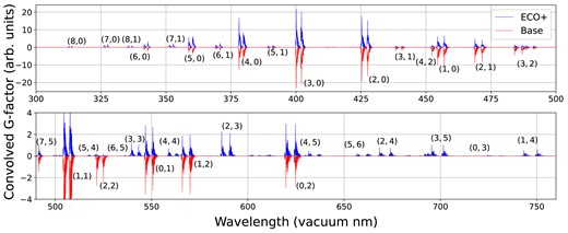
Synthetic fluorescence spectra of two CO|$^+$| models at |$v_\textrm {h} = 0$| km s|$^{-1}$| and |$r_\textrm {h} = 1$| au showing most presently included Comet Tail (A |$^2\Pi$|–X |$^2\Sigma$|) bands. The base model (red and inverted for visibility) is a recreation of the model described in Magnani & A’Hearn (1986). The expanded and updated ECO + model (blue) is produced by including up to |$v = 9$| in X |$^2\Sigma$|, |$v = 6$| in B |$^2\Sigma$|, and |$v = 8$| in A |$^2\Pi$| (see text), in addition to the newly benchmarked transition rates (Appendix A). All models are convolved with a Gaussian of 0.05 nm FWHM to increase the visibility of the bands. Band labels in the form |$(v^{\prime },v^{\prime \prime })$|, where |$v^{\prime }$| and |$v^{\prime \prime }$| are the upper and lower vibrational quantum numbers, respectively, are overlaid for select features. The (1,1) band present in all models extends beyond the restricted range shown in the figure. Both panels share a common relative intensity scale.
At this stage, it is desirable to assess how the fluorescence spectrum of CO|$^+$| is sensitive to the accuracies of the transition wavelengths. As a final check on the sensitivity of our model to the input molecular parameters, some experimentally derived constants were replaced with theoretical values from the recent quantum chemical calculations of CO|$^+$| reported in Davis, Huang & Fortenberry (2023a). These ‘Davis’ models utilized the same transition rates and structures described above, with several important constants altered. Vibrational energies, which differ by at most several cm|$^{-1}$| for X |$^2\Sigma$| and up to |$\sim$|50 cm|$^{-1}$| for A |$^2\Pi$| (increasing with v), and rotational constants B, which lie within 0.014 cm|$^{-1}$| of the values reported in Szajna, Kepa & Zachwieja (2004) for X |$^2\Sigma$| and within 0.005 cm|$^{-1}$| of the values reported in Kepa et al. (2004) for A |$^2\Pi$|, were modified accordingly. The remaining higher-order constants were fixed at the previous values. The largest impact on the fluorescence efficiencies appears to come from the excitation energy from X |$^2\Sigma$| to A |$^2\Pi$|. Using two extremes of this parameter from Davis, Huang & Fortenberry (2023a), the resulting transition wavelengths systematically shift from their ECO+ values between 0.2 to approximately 10 nm, depending on the chosen excitation energy. The band luminosities of these ‘Davis’ models differ from those of the accurate ECO + model by up to |$12\pm 17~{{\ \rm per\ cent}}$|. For the strongest bands, this wavelength inaccuracy also appears to affect the distribution of rotational states only minorly, with both the ECO+ and Davis’ models showing similar (relative) intensities of transitions within each band. These tests affirm that the present ECO + g-factors are insensitive to the accuracy of the included transition wavelengths, which appear to be in agreement with the observed bands of CO|$^+$| observed in cometary spectra (Section 5).
Lastly, these test models suggest that purely theoretical models, built on ab initio computed molecular constants, may be useful in assessing the possible contributions of currently unidentified molecules in cometary spectra. If comparable or better accuracy than that achieved for CO|$^+$| constants can also be found for other cations, such preliminary models may be useful for assessing the possible emission of these species in small body observations.
4.3 The infrared emission of CO|$^+$|
Within the B |$^2\Sigma$| and A |$^2\Pi$| states, the purely vibrational transition rates (|$A_\textrm {vib.}\sim 10^2$| s|$^{-1}$|) are much smaller than the transition rates of the Comet Tail and First Negative systems, and their inclusion is expected to have a negligible impact on the fluorescence spectrum. In the ground state, however, the level populations can be large compared to e.g. levels in A |$^2\Pi$|, which combined with the vibrational transition rates within the ground state can yield substantial infrared emission. While the pumping of the ground state vibrational bands was included in Magnani & A’Hearn (1986), who used the solar IR spectral data available in Allen (1973), the band luminosities for these bands were not reported. The present IR spectrum, which derives from the high-resolution ACE-FTS measurements (see Hase et al. 2010), provides sufficient spectral resolution to recover the velocity dependence of the infrared bands.
The ground state rovibrational bands of CO|$^+$| are approximately clustered into four wavelength windows around 1200, 1600, 2400, and 4700 nm. Fig. 2 shows synthetic fluorescence spectra computed with our ECO + model for these four IR windows containing the majority of the ground state bands. The g-factors of each band were convolved to a resolving power of |$R\sim 2000$| at 4000 nm, comparable to that of NASA’s IRTF. The band luminosities of the 20 strongest ground state vibrational bands4 included in our ECO + model are presented in Table 5 at |$r_\textrm {h} = 1$| AU and |$v_\textrm {h} = 0$| km s|$^{-1}$|. To the best of our knowledge, the present calculations provide the first quantified fluorescence efficiencies of the CO|$^+$| ground state bands. The strongest ground state emission band, (1,0), has a band luminosity approximately 1/4th that of the strongest Comet Tail band. The (1,0) band is located in the reddest window, which contains bands of the |$\Delta {v} = 1$| sequence, that is, bands described by the labels |$(v^{\prime },v^{\prime \prime }=v^{\prime }-1)$|. These bands above |$4~\mu$|m show substantial overlap and they lie within wavelength windows accessible to both NASA’s JWST with e.g. NIRSPEC, and NASA’s iShell at the IRTF. The quantification of these bands may allow for simultaneous observations of CO and CO|$^+$| emission around |$\sim$|4.7 μm, which could provide constraints on the CO/CO|$^+$| abundance and shed light on the production mechanisms of CO|$^+$| in distant comets (Womack, Sarid & Wierzchos 2017). However, the detectability of these features is not known at this time, and there exists possible overlap with known H|$_2$|O and O|$_3$| telluric absorption features (Smette et al. 2015).
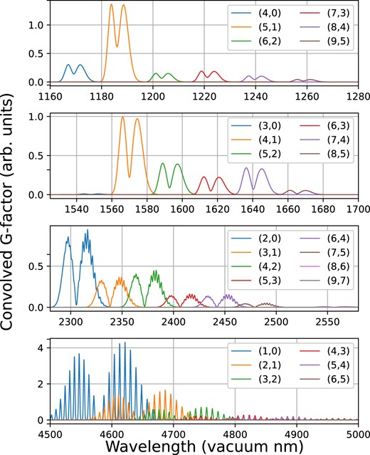
Synthetic infrared fluorescence spectra of CO|$^+$| using the ECO + model (see text). Vibrational bands within the ground electronic state are shown. g-factors are convolved with a Gaussian filter to a resolving power of |$R = 2000$| at 4000 nm. Band labels in each window are shown in the form |$(v^{\prime },v^{\prime \prime })$|, where |$v^{\prime }$| and |$v^{\prime \prime }$| are the upper and lower vibrational quantum numbers, respectively. All four panels share a common relative intensity scale.
Band Luminosities of the ground state vibrational bands (X |$^2\Sigma$|–X |$^2\Sigma$|) of CO|$^+$|. Band luminosities (|$g_\textrm {band}$|) are shown at |$r_\textrm {h} = 1$| au and |$v_\textrm {h} = 0$| km s|$^{-1}$| for the twenty strongest vibrational bands within the ground electronic state (X |$^2\Sigma$|) of CO|$^+$|. Band luminosities are provided in units of |$10^{-15}$| ergs s|$^{-1}$| molecule|$^{-1}$| as a function of the upper and lower vibrational quantum numbers |$v^{\prime }$| and |$v^{\prime \prime }$|, respectively. The maximum and minimum wavelengths of the transitions in each band are provided in vacuum nanometers, according to the ECO + model with |$N_\textrm {max} \le 20$| (see text).
| |$v^{\prime }$| | |$v^{\prime \prime }$| | |$g_\textrm {band}$| | |$\lambda _\textrm {min}$| (nm) | |$\lambda _\textrm {max}$| (nm) |
|---|---|---|---|---|
| 1 | 0 | 4.83 | 4435.72 | 4766.03 |
| 2 | 1 | 1.82 | 4497.77 | 4834.17 |
| 2 | 0 | 0.972 | 2272.72 | 2355.97 |
| 3 | 2 | 0.803 | 4561.68 | 4904.39 |
| 4 | 1 | 0.555 | 1556.82 | 1594.86 |
| 5 | 1 | 0.48 | 1179.55 | 1201.15 |
| 4 | 2 | 0.474 | 2338.1 | 2424.5 |
| 3 | 1 | 0.391 | 2304.93 | 2389.73 |
| 4 | 3 | 0.307 | 4627.45 | 4976.68 |
| 5 | 0 | 0.281 | 938.57 | 952.26 |
| 8 | 1 | 0.261 | 691.38 | 698.88 |
| 5 | 2 | 0.224 | 1579.42 | 1618.18 |
| 5 | 4 | 0.218 | 4695.07 | 5051.04 |
| 6 | 0 | 0.205 | 788.65 | 798.33 |
| 7 | 4 | 0.196 | 1626.66 | 1666.94 |
| 5 | 3 | 0.168 | 2372.21 | 2460.27 |
| 6 | 4 | 0.164 | 2407.35 | 2497.12 |
| 6 | 1 | 0.143 | 952.21 | 966.16 |
| 6 | 3 | 0.129 | 1602.69 | 1642.19 |
| 4 | 0 | 0.107 | 1162.79 | 1183.98 |
In the remaining three windows, the IR bands are relatively weak, and exhibit minimal overlaps at the extremes of their spectral ranges. We note that these fluorescence efficiencies may be subject to large uncertainties, owing to at-times large differences between vibrational transition rates from Rosmus & Werner (1982) and Qin, Zhao & Liu (2017). While our normalization solution attempts to minimize errors introduced by combining transition rates between these authors (see Section 2.3), the fluorescence efficiencies of the ground state bands of CO|$^+$| should be considered to have large uncertainties at this time. Further calculations or benchmarking experiments may be required to more accurately quantify the infrared emission of CO|$^+$|.
4.4 Heliocentric velocity and distance dependencies of CO|$^+$| emission
In the fluorescence rate equations (equation 1), the absorption rates |$W = \rho {B}$| are inversely proportional to the square of the heliocentric distance |$r_\textrm {h}$|. For a fixed distance, the radiation field |$\rho$| is sensitive to the heliocentric velocity via the Swings effect (Swings 1965), where the comet’s velocity with respect to the Sun results in an effective Doppler shift of the exciting solar radiation.
To investigate the heliocentric velocity dependence of the electronic bands of CO|$^+$|, we computed the band luminosities (at 1 AU) on a grid of heliocentric velocities spanning −50 to +50 km s|$^{-1}$|. In Magnani & A’Hearn (1986), band luminosities are reported for the Comet Tail bands, with typical variations over the velocity space of |$\sim \pm 10~{{\ \rm per\ cent}}$|. Fig. 3 shows the luminosities of the Comet Tail, First Negative, and ground state bands of CO|$^+$|, normalized to their values at |$v_\textrm {h} = 0$| km s|$^{-1}$| as a function of heliocentric velocity. Over the velocity range of -50 to + 50 km s|$^{-1}$| the Comet Tail band luminosities change by at most 15 per cent, with the majority of bands changing by |$\pm$|5 per cent.
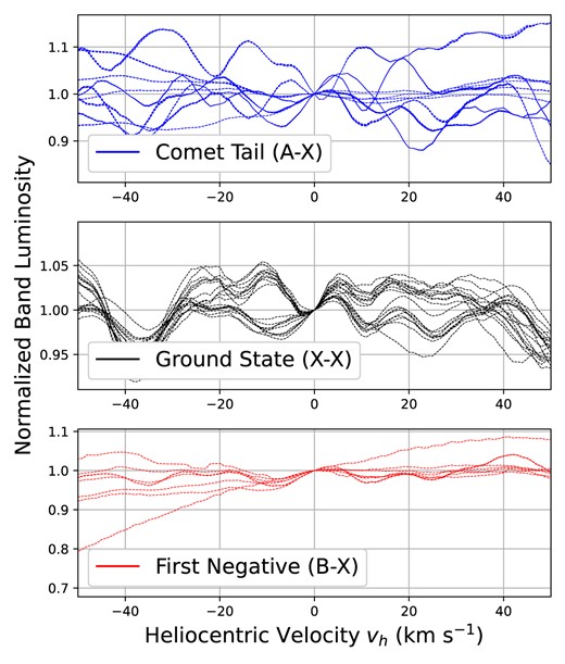
Heliocentric velocity dependencies of the Comet Tail bands (top), ground state vibrational bands (middle), and First Negative bands (bottom) at |$r_\textrm {h}$| = 1 au. Each band included in the ECO + model is shown normalized to a value of 1 at |$v_\textrm {h} = 0$| km s|$^{-1}$|. Velocity-dependent band luminosities are provided as supplementary information.
To the best of our knowledge, the present calculations include the first investigations of the velocity dependence of the First Negative and ground state bands of CO|$^+$|. The majority of the ground state vibrational bands exhibit a common oscillatory behaviour with changing velocity. The absolute magnitudes of the bands change little as a function of velocity, approaching only 4–5 per cent in the extremes of the considered velocity space. This is not surprising, as the rovibrational levels of X |$^2\Sigma$| are simultaneously connected by many strong allowed transitions to the A |$^2\Pi$| and B |$^2\Sigma$| states. As noted by Magnani & A’Hearn (1986), the solar IR spectrum is also relatively smooth. Combined, these two facts suggest one can expect a weak dependence of the ground state band emission on heliocentric velocity, consistent with the present calculations.
The largest variations in the CO|$^+$| band luminosities, as a function of heliocentric velocity, are observed in the First Negative system, primarily at large, negative, velocities. Over a majority of the present velocity range, the typical variations are of order |$\pm 10~{{\ \rm per\ cent}}$|. We note that the Baldet–Johnson bands, being produced by decays of the same states which produce the First Negative bands, show identical heliocentric velocity behaviour as the First Negative system and are not shown.
It is convenient in spectral analyses to compute fluorescence efficiencies at |$r_\textrm {h} = 1$| AU and scale the g-factors to the heliocentric distance of an observed object by |$g(r = 1~\textrm {AU})\times 1/r^2_\textrm {h}$|. As the incident solar radiation scales as |$1/r^2_\textrm {h}$|, so do the absorption rates, potentially impacting the rate equations which determine the level populations and fluorescence efficiencies.
We investigated the heliocentric distance dependence of the CO|$^+$| fluorescence efficiencies. Fig. 4 shows the ratios of each band luminosity computed at 1 au and scaled by |$1/r_\textrm {h}^2$| and the same band luminosities computed by explicitly including the 1/|$r^2$| decrease in the absorption rates. The Comet Tail band luminosities are relatively unaffected by the explicit |$r_\textrm {h}$| dependence of the absorption rates. At the extremes of the parameter space, |$r_\textrm {h} = 0.1$| au and |$r_\textrm {h} = 10$| au, the band luminosities typically differ by 10–15 per cent between |$r_\textrm {h}$|-dependent and 1-au-scaled g-factors. Purely rotational transitions in the ground vibrational level (|$v=0$|) show a stronger dependence, up to a factor of 3 at |$r_{\textrm {h}} = 0.1$| AU. The remaining purely rotational transitions in higher vibrational states show large variations as a function of |$r_\textrm {h}$|, but their band luminosities and impact on the models are negligible. Different trends are identified in the First Negative bands, with some bands showing more extreme changes between 1 au and |$r_\textrm {h}$|-dependent g-factors as |$r_\textrm {h}$| deviates from 1 au. However, the strongest First Negative bands show trends comparable to the Comet Tail system.
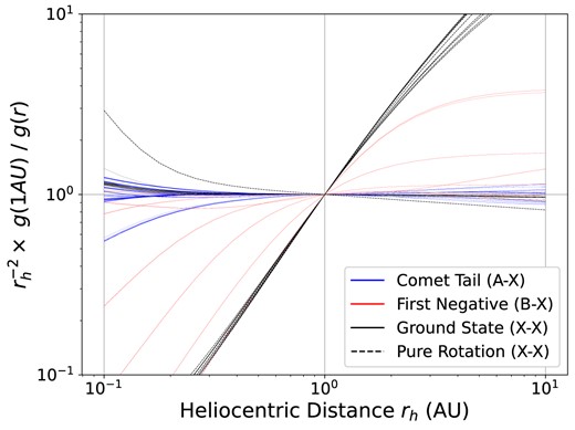
Ratios of the band luminosities at 1 AU scaled by |$1/r^2_\textrm {h}$| and the band luminosities as a function of heliocentric distance |$r_\textrm {h}$|. All bands in the Comet Tail (blue), First Negative (red), and ground state (black) systems are shown. Purely rotational transitions in the ground state (|$v^{\prime } = v^{\prime \prime }$|) are shown with a dashed line, with rovibrational (|$v^{\prime } \ne v^{\prime \prime }$|) transitions shown with solid black lines. All fluorescence efficiencies and band luminosities are calculated with the ECO + model (see text).
As the absorption rate scales as |$1/r_\textrm {h}^2$|, at large heliocentric distances the absorption rates can become smaller than the transition rates within the ground electronic state. Thus the distribution of rotational states in X|$^2\Sigma$| that are pumped to A|$^2\Pi$| are expected to evolve as a function of |$r_\textrm {h}$|, as well as the relative intensities of emission lines within each band. Fig. 5 shows the synthetic spectra of the Comet Tail (3,0) band, convolved to a spectral resolution of 0.05 nm FWHM, at |$v_\textrm {h} = 0$| km s|$^{-1}$| and three heliocentric distances (0.1, 1, and 10 au). The spectra are normalized to a maximum value of one within each model to highlight changes to band shape. At 0.1 au, a larger number of rotational states in A |$^2\Pi ~(v=3)$| are populated, resulting from the widened distribution of rotational states within X |$^2\Sigma$|. With increasing distance, the band luminosity is dominated by a smaller number of (relatively) stronger transitions. While the band luminosity scales approximately as |$1/r_\textrm {h}^2$|, the g-factors of individual transitions can show much larger variations. As a test of the assertion that the ground state rovibrational transitions are responsible for producing the sensitivity to heliocentric distance, we pursued fluorescence calculations where the transitions within the ground state were completely removed. In the resulting band luminosities, no sensitivity to heliocentric distance is observed up to the largest distance explored here (10 au). Further, models without transitions within X|$^2\Sigma$| result in poor agreement with observations available to us, as these transitions are pivotal in the determining the populations within the ground state.
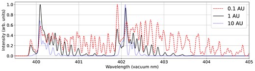
Synthetic spectra of the Comet Tail (3,0) band generated with the ECO + model (see text) at fixed |$v_\textrm {h} = 0$| for heliocentric distances of 0.1 (red dashed), 1 (solid black), and 10 au (dotted blue). All spectra are convolved to a resolution of 0.05 nm FWHM and normalized to a maximum value of one within each model.
Summarizing, the re-scaling of band luminosities from 1 au does not appreciably affect the band luminosities. Re-scaling band luminosities from 1 au to a distance |$r_\textrm {h}$| is appropriate, in the case of CO|$^+$|, when one is interested in extracting column densities by integrating over entire spectral bands. However, the use of 1-au scaled g-factors for individual transitions is inappropriate, as they do not scale readily with |$1/r_\textrm {h}^2$| and are likely to provide a poor match to observed spectra at |$r_\textrm {h} \ne 1$| au.
4.5 Time-dependence of CO|$^+$| emission
In routine calculations of fluorescence efficiencies, it is typically assumed that |$dn/dt = 0$|, i.e. that enough time has elapsed such that the observed emission is from species in fluorescence equilibrium. While this greatly simplifies the calculation of fluorescence efficiencies, it may not be always be appropriate. Using the modified time-dependent capabilities of the fluorescence model (Section 2), we investigated the validity of this assumption for CO|$^+$|. As the number of computational steps scales roughly as the product of the number of transitions and the number of time steps, it is first beneficial to reduce the computational demands by including only the relevant states and associated transitions. We restrict our time-dependent calculations to a model including |$v\le$| 9, 2, and 6 for the X |$^2\Sigma$|, B |$^2\Sigma$|, and A |$^2\Pi$| states respectively, each with rotational states up to |$N = 10$|. Comet Tail Band luminosities calculated with this reduced model differ from the full ECO + results (Table 2) by |$\lt 0.3~{{\ \rm per\ cent}}$|.
It is worth noting that the time dependence of the fluorescence efficiency (equation 8) is separate from a hypothetical time duration of an astrophysical observation. Once produced, we assume that CO|$^+$| is formed in the lowest vibrational and rotational level in X |$^2\Sigma$|. Starting with unit population, the CO|$^+$| evolves over some length of ‘fluorescence time’, in which the populations develop according to the time-dependent balance of absorption and spontaneous emission. As real cometary observations are observing a distribution of CO|$^+$| at various stages of fluorescence time evolution, analysis of real spectra time-dependently would require coupling of the time-integrated fluorescence efficiencies to an involved model of the CO|$^+$| density distribution. We defer the coupling to a density distribution model to a future work.
If the emitting species fails to attain equilibrium within the time frame where the emitter remains in the field of view, it may be essential to consider time-dependent fluorescence efficiencies. While each transition develops in time differently, some commonalities are found in the time evolution of the CO|$^+$| fluorescence efficiencies. Fig. 6 shows instantaneous time-dependent fluorescence efficiencies for strong bands in each of the Comet Tail, First Negative, and ground state systems at |$r_\textrm {h} = 1$| au and |$v_\textrm {h} = 0$| km s|$^{-1}$|. At |$t=0$|, both the Comet Tail and First Negative band luminosities begin within |$\sim 10~{{\ \rm per\ cent}}$| of their equilibrium values, and asymptotically approach their equilibrium values between 100 and 1000 s. With increasing time, these bands redistribute population amongst the vibrational levels of X |$^2\Sigma$|, increasing the g-factors for the ground state vibrational bands. This results in a brief over-population of the ground state vibrational levels, which subsequently decay or act as additional drivers of excited state population as the system develops toward equilibrium.
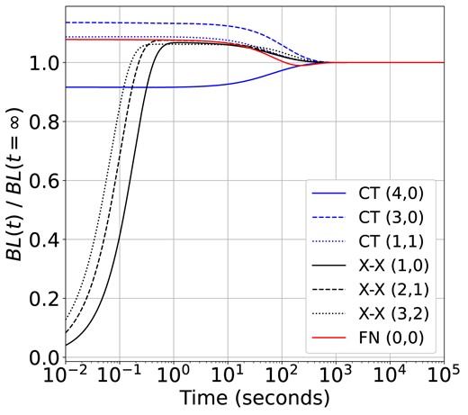
Ratio of time-dependent band luminosities to their equilibrium values for select bands of the Comet Tail (CT), First Negative (FN), and ground state vibrational systems (X-X) for |$r_\textrm {h} = 1$| au and |$v_\textrm {h} = 0$| km s|$^{-1}$|.
In our investigation of the time dependence of CO|$^+$| emission, it became useful to define an ‘equilibrium time-scale’ |$t_\textrm {eq.}$| after which a time-dependent approach is indistinguishable from an equilibrium g-factor calculation. A first choice of this arbitrary time-scale is the time at which the strongest band of CO|$^+$| has achieved an instantaneous time-dependent band luminosity within 10 per cent of its equilibrium value. This instantaneous band luminosity is produced by summing equation (7) over the transitions in each band. This choice is motivated by the expected uncertainties in the flux calibrations of reported observations of CO|$^+$| emission in comets (Korsun, Ivanova, & Afanasiev 2006; Ivanova et al. 2016; Cochran & McKay 2018), and a more rigorous criterion can be coupled with more precise measurements.
The equilibrium time-scales of strong bands in each system are shown for a range of heliocentric distances and velocities in Fig. 7 (top row). In general, the Comet Tail equilibrium time-scale |$t_\textrm {eq.}$| increases with distance from |$\sim$|100 s at 1 au to |$\sim$|3000 s at 10 au. The ground state (1,0) band quickly (|$\lt 1$| s) approaches its equilibrium band luminosity even up to |$r_\textrm {h} = 10$| AU, though the X|$^2\Sigma (v=1)$| rotational populations continue to develop over longer time-scales. Higher vibrational states within X|$^2\Sigma$| exhibit much longer equilibrium time-scales, comparable to the excited A|$^2\Pi$| and B|$^2\Sigma$| states. For a fixed distance, the equilibrium time-scales also show a sensitivity to heliocentric velocity. Fig. 7 (top left) shows the equilibrium time-scales for the Comet Tail (3,0) band. For some velocities, the band luminosity quickly (|$\sim$|seconds) achieves a band luminosity close to its equilibrium value, while other velocities require a few thousand seconds to equilibrate, owing to the complexity of the solar spectrum. The First Negative system shows similar trends, with a relatively reduced sensitivity to heliocentric velocity.
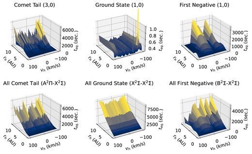
(Top row) Equilibrium time-scales of select CO|$^+$| emission bands, calculated as the time at which the instantaneous band luminosity is within 10 per cent of the equilibrium value (see text). A color gradient, mapped to the equilibrium time in each plot, is shown for visual clarity. (Bottom row) Equilibrium time-scales for all bands of the Comet Tail (A |$^2\Pi$|-X |$^2\Sigma$|) (bottom left), ground state (X |$^2\Sigma$|- X |$^2\Sigma$|) (bottom middle), and First Negative (B |$^2\Sigma$|- X |$^2\Sigma$|) band systems (bottom right).
Using an equilibrium time-scale |$t_\textrm {eq.}$| derived from individual bands is not useful if one is motivating the application of time-dependent versus equilibrium fluorescence efficiencies, as the time-scale will depend critically on which bands are used. The results of a potentially more meaningful definition of |$t_\textrm {eq.}$| are shown in Fig. 7 (bottom row), where |$t_\textrm {eq.}$| is defined as the time-scale at which all bands of each system have achieved a luminosity within 10 per cent of their equilibrium values. With this definition of |$t_\textrm {eq.}$|, all three band systems show similar trends with |$r_\textrm {h}$|, with minor variations superimposed from the differing velocity-dependent absorption rates. Further, the distribution of features within each band may change dramatically as a function of time, while the rotational populations within X|$^2\Sigma$| are redistributed, even while the time-dependent band luminosity is close to its equilibrium value. As will be motivated below, in the absence of spatial distribution models of CO|$^+$|, we restrict our model comparisons with comet observations to equilibrium fluorescence models, but note that time-dependent effects may become important near the nucleus.
5 BENCHMARKING AND DISCUSSION
5.1 Benchmarking against cometary spectra
The present fluorescence emission model of CO|$^+$| utilizes updated molecular constants and spectroscopic parameters collected from recent experimental and theoretical efforts. As a test of this fluorescence model, we calculated equilibrium fluorescence efficiencies at the orbital conditions of C/2016 R2 (PanSTARRS), hereafter ‘R2’, during the observations carried out by Cochran & McKay (2018), |$r_\textrm {h} = 3.05$| au and |$v_\textrm {h} = -9.85$| km s|$^{-1}$|. Fig. 8 shows comparisons of several observed CO|$^+$| bands from Cochran & McKay (2018) and our fluorescence models convolved to the observational resolution (|$R \sim 60\, 000$|). From Fig. 8, we find good agreement between the fluorescence model and the majority of the observed fluxes of the Comet Tail bands in R2. However, each band is observed in a different echelle order, and cross-order comparisons of relative intensities is difficult. Within an order, there are at times minor differences between the observed and modelled wavelengths owing to the wavelength calibration, as evidenced by the residuals for e.g. the (1,1) band. We also note that the fluorescence model is arbitrarily scaled to the red branch of each band, which can degrade the agreement between the model and observed spectrum in the blue branches. Despite these complications, the observed features are well described by our equilibrium fluorescence model. Based on the differences in our band luminosities utilizing different solar spectra (10 per cent), the expected accuracy of the intensity calibration in our benchmarking procedure (|$\sim$|15 per cent), and the quoted uncertainties of the lifetimes used to normalize our transition rates (5 per cent), we expect our g-factors are accurate at the |$\sim$|20 per cent level, consistent with the level of agreement for most transitions in Fig. 8.
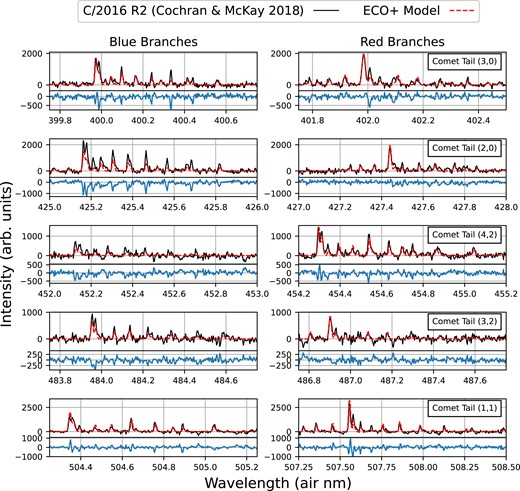
Comparisons of the ECO + fluorescence model convolved to |$R = 60\, 000$| to the Comet Tail bands of C/2016 R2 (PanSTARRS) observed by Cochran & McKay (2018). The comet spectra were acquired with the Tull 2DCoude spectrograph on the Harlan J. Smith 2.7 m telescope at the McDonald Observatory between 2017 December 8 and 10 (Cochran & McKay 2018). The ECO + model was used to generate fluorescence efficiencies at |$r_\textrm {h} = 3.06$| au and |$v_\textrm {h} = -9.8$| km s|$^{-1}$|. As the relative flux calibration between the echelle orders used to observe the Comet Tail bands is difficult to establish, each band is arbitrarily scaled to match the strongest feature in the red branch of the CO|$^+$| band present in each order. Residuals showing (Model – Data) are shown beneath each band in blue.
Historically, CO|$^+$| has been invoked to explain the famous ‘Comet Tail’ emission features (Fowler 1909; Swings 1965). In such cases, one might expect a predominantly fluorescence origin owing to the tenuous nature of the comet tail structures. The observations of C/2016 R2 (PanSTARRS) carried out by Cochran & McKay (2018) and Opitom et al. (2019) sampled cometocentric distances |$r \lt 12\, 000$| km. From the photo-chemical modeling presented in Raghuram et al. (2020), photo-ionization, electron impact ionization, and charge exchange between C|$^+$| and CO|$_2$| contribute to the production and possibly the excitation of CO|$^+$|. From their ionic production models, Raghuram et al. (2020) also found that the photochemical lifetime of CO|$^+$| is |$\sim$|2000 s at 10 000 km, a factor of |$\sim$|few larger than the present equilibrium time-scales, suggesting that time-dependent effects may present a possible complication, depending on the spatial distribution of the emitting CO|$^+$|. At this time, we cannot rule out contributions from additional excitation mechanisms, though the observed spectra appear consistent with our model assuming fluorescence equilibrium. A combination of collisional excitation mechanisms and time-dependent effects may be explored in future work.
Spectra collected with a larger field of view, where both collisional and time-dependent effects are expected to be greatly diminished, may offer additional benchmarks for the present fluorescence efficiencies. Several such spectra are available for the peculiar comet 29P/Schwassmann–Wachmann 1, which is well known for its rich CO atmosphere and frequent outburst activity (Wierzchos & Womack 2020). Fig. 9 shows comparisons of the present ECO + model to two observations of 29P which sample different orbital conditions, approximately |$v_\textrm {h} = \pm 0.5$| km s|$^{-1}$|. Spectra collected at |$v_\textrm {h} = -0.47$| km s|$^{-1}$| are available from observations in 2016 August using the 4.1 m SOAR telescope (Ivanova et al. 2018), which sampled cometocentric distances up to |$\sim 10^6$| km. While these spectra are lower resolution than the R2 observations discussed previously, the observed bands are on the same relative intensity scale, allowing for checks of all observed bands simultaneously. Agreement is found with the majority of the CO|$^+$| bands present in the SOAR spectra. Comparisons to spectra of 29P at |$v_\textrm {h} = +0.49$| km s|$^{-1}$| from Korsun, Ivanova & Afanasiev (2008), collected with the 6 m BTA (Fig. 9 bottom panel) show improved agreement relative to the SOAR observations, likely owing to the improved signal to noise in the BTA observations. As an example, the modelled band luminosities for the (1,1) (chosen as the (1,0) band is blended with the (4,2) band, though the blend appears well described), (2,0), and (3,0), bands compare favourably with the observed spectrum. The modelled luminosity ratios of the three bands, 1:2.3:3, are in excellent agreement with the observed flux ratios (produced by integration over the observed bands) of 1:2.4:3.3 in the BTA observations. Lastly, the modelled (4,0) band appears to be broader and stronger in the model compared to the observations. This finding is consistent with degradation of the signal to noise as one progresses deeper into the ultraviolet.
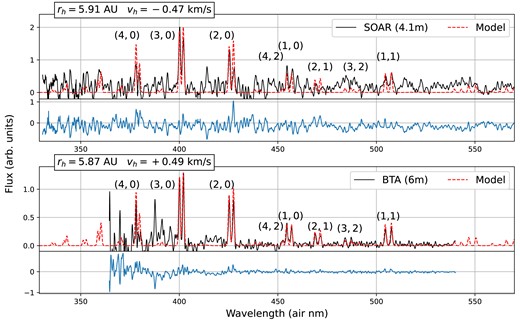
Comparisons of the ECO + model to observed spectra of 29P/Schwassmann–Wachmann 1. (Top) Comparisons to the observations of Ivanova et al. (2018) collected at orbital conditions |$r_\textrm {h} = 5.91$| au and |$v_\textrm {h} = -0.47$| km s|$^{-1}$| on 2016 August 12 using the 4.1 m Southern Astrophysical Research Telescope (SOAR) telescope. (Bottom) Comparisons to the observations of Korsun, Ivanova & Afanasiev (2008) collected at orbital conditions |$r_\textrm {h} = 5.87$| AU and |$v_\textrm {h} = +0.49$| km s|$^{-1}$| using the 6 m Large Azimuth Telescope (Bolshoi Teleskop Alt-azimutalnyi, ‘BTA’) on 2006 December 15–16. Models are convolved with a Gaussian to a spectral resolution comparable to the observations and arbitrarily scaled to the (3,0) band around 400 nm. Residuals (Model – Data) are shown beneath each band in blue. Labels for strong Comet Tail bands are shown.
In total, the comparisons between the spectra of 29P and C/2016 R2 (PanSTARRS) validate the relative fluorescence efficiencies of our updated CO|$^+$| model. In the high-resolution spectra of C/2016 R2 (PanSTARRS), we find good agreement between the observed distributions of individual transitions within bands and those predicted by our ECO + model. However, the data span multiple echelle orders and are not on the same relative flux scale. In the lower-resolution observations of 29P taken with the SOAR and BTA teslecopes (Korsun, Ivanova & Afanasiev 2008; Ivanova et al. 2018), we find excellent agreement between the fluxes of numerous observed CO|$^+$| bands, and the predictions of our pure-fluorescence model. Future efforts will investigate the incorporation of the present fluorescence model into density-dependent production models which include multiple excitation mechanisms. Such models will require collision data (cross-sections) for the relevant processes, including electron impact excitation and/or dissociative excitation, photodissociation, charge exchange, and possibly collisions with other volatiles.
During the review of this manuscript, Rousselot et al. (2023) also reported a similar fluorescence model of CO|$^+$| used to characterize the CO|$^+$| bands observed in high-resolution spectra of C/2016 R2 (PanSTARRS), taken with the European Southern Observatory Very Large Telescope. A comparison of our models against figures in Rousselot et al. (2023) shows similar levels of agreement in describing the rovibrational structure of the bands. Our flux ratio of the (3,0)/(4,0) bands, 1.5, is similar to the value of 1.63 reported in Rousselot et al. (2023). The present fluorescence efficiencies of the (3,0) and (4,0) band luminosities are |$\sim 40~{{\ \rm per\ cent}}$| larger than the values in Rousselot et al. (2023). The present band luminosity ratios for the (1,1), (2,0), and (3,0) bands, |$1:2.16:2.8$|, agree well with the fluxes observed at 29P, having ratios |$1:2.32:3$|. In comparison, from the tables of Rousselot et al. (2023), one finds the band luminosity ratios |$1:1.6:2$| appearing slightly at odds with the observations of 29P. However, such comparisons are sensitive to the normalization, in this case to the (1,1) band. Comparing the ten strongest bands reported in Rousselot et al. (2023) to the present results (Table 2), one finds band luminosities differing by only |$\sim$|30 per cent. As these differences are larger than those expected from the use of different solar flux atlases (Section 3), they are likely driven by the transition rates utilized in the respective works.
5.2 Implications
Lastly, we briefly examine implications of the updated CO|$^+$| fluorescence efficiencies. Historically, many of the derivations of CO|$^+$| column densities from observed CO|$^+$| in comets have relied on the use of a single band. For example, Lutz, Womack & Wagner (1993) derived the CO|$^+$| column density for comets 1P/Halley and 1C/1987 P1 (Bradfield) using the g-factor of the Comet Tail (2,0) band reported by Magnani & A’Hearn (1986). From Table 2, we find the ECO + model produces a g-factor 5 per cent smaller. Ignoring the dependence on heliocentric distance, which are close to 1 au for both comets, this suggests a minor change in derived CO|$^+$| abundance. However, other bands, in particular the strong (4,0) band, can show large differences between the previous work of Magnani & A’Hearn (1986) and the present results.
In some cases, N|$_2^+$| emission was observed simultaneously with CO|$^+$| bands, allowing for measures of N|$_2^+$|/CO|$^+$| abundances which in turn can shed light on the N|$_2$|/CO abundance and conditions present during comet formation. To-date, these derivations relied on the CO|$^+$|g-factors reported in Magnani & A’Hearn (1986). As discussed above, the present g-factors provide an update and expansion of those reported in Magnani & A’Hearn (1986). Using the updated fluorescence efficiencies from the ECO + model (Table 2) could modify published N|$_2$|/CO abundances derived from cation emission bands. An N|$_2$|/CO abundance of 0.06 was previously derived for C/2016 R2 (PanSTARRS) (Cochran & McKay 2018; Opitom, C. et al. 2019), 0.002 for 1P/Halley Womack, Wyckoff & Ziurys (1992), and 0.02 in 1C/1987 P1 (Bradfield) (Lutz, Womack & Wagner 1993). Using the updated N|$_2^+$| fluorescence efficiencies reported in Rousselot, P. et al. (2022) and the present CO|$^+$| results, the revised N|$_2$|/CO ratios for these comets are 0.041 (−32 per cent), 0.0015 (−23 per cent) and 0.0158 (−22 per cent), respectively. Future N|$_2$|/CO derivations should, where possible, utilize multiple CO|$^+$| bands in order to minimize sensitivity to inaccuracies in individual band luminosities, particularly for distant comets. The derivation of N|$_2$|/CO from N|$_2^+$|/CO|$^+$| ratios also relies on the assumption of a single ionization mechanism for both N|$_2$| and CO i.e. photoionization. Multiple ionization and/or excitation mechanisms may contribute to the production and emission of CO|$^+$|, and further work is required to understand these mechanisms for cometary CO|$^+$| and possibly for N|$_2^+$| as well.
6 CONCLUSIONS
We report new fluorescence emission models of the carbon monoxide cation, CO|$^+$|. Using the PGOPHER software and a compilation of experimentally derived, accurate molecular constants, we computed a line list of all rovibronic transitions between the first three electronic states of CO|$^+$|. The CO|$^+$| line and energy level lists are used as inputs to a modified version of the FlorPy model described in Bromley et al. (2021), with extension to the time domain. Using the fluorescence model code and our CO|$^+$| line lists, we developed several fluorescence models with increasing complexity and accuracy. As a test case, a ‘base’ model, acting as a recreation of the fluorescence model described in Magnani & A’Hearn (1986), was developed, and produces fluorescence efficiencies of the Comet Tail (A |$^2\Pi$| - X |$^2\Sigma$|) bands within 12 per cent of those reported in Magnani & A’Hearn (1986).
An updated, recommended fluorescence model, labelled ‘ECO + ’, was constructed by expanding the number of rotational and vibrational states, and updating the transition rates with a set which has been benchmarked against new laboratory spectra (see Appendix A). Using our updated model, we investigated the velocity, distance, and time dependence of CO|$^+$| emission features, and associated implications for analyses of comet spectra. The results may be summarized as follows:
Our model code has been made available on GitHub, and the model code and outputs are being prepared for storage in permanent archives, including Zenodo and NASA’s Planetary Data System. Numerous supplementary files, including line lists, PGOPHER input files, and modelled fluorescence efficiencies are provided as supplementary files to this manuscript.
Increasing the number of included states modifies the rate equations, with increases in the number of vibrational states in X |$^2\Sigma$| having the largest effect on the fluorescence efficiencies of the Comet Tail system. The expanded model, ECO +, predicts several (new) possibly observable Comet Tail bands between 500 and 750 nm which were identified in C/2016 R2 (PanSTARRS) by Rousselot et al. (2023).
We report, for the first time, absolute fluorescence efficiencies for the ground state vibrational bands of CO|$^+$|, the majority of which are clustered into approximately four spectral windows around 1200, 1600, 2400, and 4700 nm. We suggest that additional calculations and/or experimental measurements should be made to improve the accuracy of the vibrational transition rates within the X |$^2\Sigma$| state of CO|$^+$|.
On average, the ground state, Comet Tail, and First Negative systems exhibit only slight (|$\sim 10~{{\ \rm per\ cent}}$|) fluctuations in band luminosity with respect to heliocentric velocity for a given distance from the Sun.
For CO|$^+$|, the use of band luminosities computed at 1 au and scaled to the heliocentric distance of an observation is only appropriate for deriving column densities from fluxes produced by summing over a band. Fluorescence efficiencies for individuals transitions should not be scaled from 1 au in order to interpret high-resolution spectra, as they exhibit large differences when compared to models where absorptions rates are explicitly dependent on |$r_\textrm {h}$|.
Using our time-dependent model and a well-defined equilibrium time-scale |$t_\textrm {eq.}$|, we explicitly calculate the time-scale for fluorescence equilibrium for all emission bands of CO|$^+$|. Individual bands show large scatter in |$t_\textrm {eq.}$| as a function of heliocentric velocity and distance. An equivalent time-scale derived from all bands of a given system simultaneously predicts equilibrium time-scales ranging from several hundred seconds at |$r_\textrm {h} = 1$| au to several thousand seconds at |$r_\textrm {h} = 10$| au.
Comparisons of the present ECO + fluorescence model to observations of C/2016 R2 (PanSTARRS) reported in Cochran & McKay (2018) show good agreement in describing the distribution of intensities within individual Comet Tail bands. Equilibrium fluorescence efficiencies, computed with our ‘ECO + ’ model, show excellent agreement with the low-resolution spectra of 29P reported in Korsun, Ivanova & Afanasiev (2008) and Ivanova et al. (2018), which sampled up to large cometocentric distances (|$\sim 10^6$| km). These comparisons validate the relative intensities of the CO|$^+$| bands predicted by our model.
Replacing the Magnani & A’Hearn (1986) fluorescence efficiencies with updated values (with explicit |$r_h$|-dependence) from the present ECO + model, in addition to refined N|$_2^+$| band luminosities from Rousselot et al. (2022) can lead to up to 20–30 per cent changes in established N|$_2$|/CO abundance ratios. We suggest that the community should, where possible, utilize both sets of updated g-factors in deriving abundances, as well as consideration of multiple CO|$^+$| bands in deriving abundance ratios, particularly in distant comets when certain bands may be sensitive to minor heliocentric distance-dependent effects.
Future work will explore the development of a model incorporating collisional- and time-dependent effects for analysing near-nucleus spectral observations of CO-rich comets which exhibit CO|$^+$| emission.
ACKNOWLEDGEMENTS
This paper includes data taken at The McDonald Observatory of The University of Texas at Austin, and the Southern Astrophysical Research (SOAR) Telescope. We extend our sympathies for the passing of Colin Western, whose efforts in developing, maintaining, and expanding the use of the PGOPHER software are unmatched. We also wish to extend our thanks to Peter Bernath, who provided many insights into the present use of PGOPHER for producing line lists of CO|$^+$|. The authors extend their thanks to Z. Qin for providing their computed transition rates of CO+. The authors gratefully acknowledge the expertise and computing resources provided by the Easley computing cluster and the Auburn University High Performance Computing team. Authors SB, DB, BS, and JO are grateful for funding from Europlanet grant #21-EPN-FT1-015 which enabled the electron impact experiments used to benchmark data presented in this manuscript.
DATA AVAILABILITY
Line and level lists, sample model outputs, and associated files are provided in the online supplementary files. The fluorescence model code is freely distributed on GitHub at https://github.com/StevenBromley/fluorescence_model. The model code and input files are also published on Zenodo (https://zenodo.org/records/10520441) and the NASA Planetary Data System (doi:10.26007/ZRM5-CG86).
Footnotes
doi:10.26007/ZRM5-CG86
Band luminosities for all bands included in the model are available as supplementary files.
References
APPENDIX A: EXPERIMENTAL BENCHMARKING
Once excited, a vibrational level, |$v^{\prime }$| of the upper electronic state involved in a transition can decay to numerous vibrational levels |$v^{\prime \prime }$| in the lower electronic state. The relative intensities of these bands are proportional to |$A_{v^{\prime },v^{\prime \prime }}/\sum _{v^{\prime \prime }}A_{v^{\prime },v^{\prime \prime }}$|, where |$1/\sum _{v^{\prime \prime }}A_{v^{\prime },v^{\prime \prime }}$| is more formally known as the lifetime |$\tau$|. Borrowing the expression for the g-factor (equation 2), the intensity of an observed emission line can be expressed as (ignoring geometric factors and assuming photon units):
where |$n_{v^{\prime }}$| is the population of the upper vibrational level and |$A_{v^{\prime },v^{\prime \prime }}$| is the transition rate of the band. The observed intensities of two bands from the same upper vibrational level, labelled as bands one and two for convenience, can be written as
Thus, when more than one band from the same upper vibrational level are observed simultaneously, their relative intensities, calculated as the integral over the spectral extent of the bands, can be used to constrain the ratios of the two transition rates A. If many such bands can be observed, their relative intensities can be used to derive the ratios |$A_1/A_2$|, and experimentally measured lifetimes |$\tau$| can be used to place the sum of these transition rates onto absolute scale.
In order to apply the above procedure to calibrate the transition rates of the Comet Tail system, the emission of CO|$^+$| was observed in crossed-beam experiments at the Electron Induced Fluorescence Laboratory at Comenius University, Bratislava, Slovak Republic. The experimental apparatus is described in detail in Blaško et al. (2023), Danko et al. (2013), and references within. To summarize, an electron beam is energy-monochromatized to a FWHM of |$\sim$|0.5 eV, and crossed with a neutral beam generated by expansion of a gas from a capillary tube. Photons originating from the |$e^-+$|CO collisions are focused into the entrance slit of an optical monochromator. We utilized here a photomultiplier detector sensitive in the UV region from 200 to 600 nm. The recent addition of a CCD detector to the system has also allowed for fast measurement of the emission spectrum between |$\sim$|290 and 1000 nm, which was measured at energies between 2.5 and 100 eV electron energy. The wavelength scales are calibrated by observations of standard sources. Calibration of the relative intensity scale is carried out by comparing emission features of known N|$_2$| bands and a thermal black-body source, which consisted of a heated tungsten filament mounted within the vacuum chamber. Single collision conditions were ensured by operating the system in the region where the photon count rate was linearly proportional to the target gas pressure. A manuscript describing the sum total of the electron impact experiments and the measured emission cross-sections is in preparation (Stachová, in prep.).
For the present purposes, we utilized the spectrum collected at 50 eV electron energy with the PMT detector to calibrate the vibrational transition rates of the Comet Tail system. While neutral CO bands are observed beneath the threshold for ion formation, their cross-section decreases with energy, and the CO|$^+$| bands rise sharply above the ionization-excitation threshold of |$\sim$|18 eV. Further, the CO bands occur at different wavelengths than the CO|$^+$| bands, allowing for an estimation of the CO contamination in each CO|$^+$| band. We expect little to no contribution from neutral CO bands at the wavelengths of the CO|$^+$| bands of interest at 50 eV electron energy. Lastly, the CCD spectrum between 300 and 1000 nm was used to check for additional strong bands in the region beyond the PMT’s spectral range. No strong bands which could affect our re-calibration efforts were noted, though many weak bands of CO|$^+$| are identified in this region.
The transition rates were calibrated by an iterative procedure as follows. First, the bands present in the spectrum were identified by comparisons with our theoretical model built on the transition rates of Qin, Zhao & Liu (2017). For each upper level, the spectral extent of each related band was identified with the aid of the theoretical model, and the intensities of the bands were computed as an integral over the extent of each band. Additionally, the vibrational level population is extracted from each band that is free of blends. Corrections for travel outside the field of view before radiative decays occur were applied using the measured lifetimes of Möhlmann & De Heer (1976). Second, band transition rates were manually adjusted, vibrational populations re-derived and used to re-weight the synthetic spectrum, and the process is repeated until agreement is achieved with the experimental spectrum. For bands which were not observed due to the limited bandpass of the PMT their transition rate ratio to the strongest band sharing a common upper level was fixed. This process was also repeated for the First Negative and Baldet–Johnson systems, allowing for benchmarking of transition rates for the strongest bands of each system.
In each iteration of the benchmarking procedure, the placement of the transition rates onto an absolute scale was carried out as follows. For each upper vibrational level, the sum of the calibrated/scaled transition rates (with respect to the strongest transition in each band) is renormalized according to the measured lifetimes of the A |$^2\Pi$||$(v = 0 - 8)$| levels as reported in Möhlmann & De Heer (1976). The same process was applied for all First Negative and Baldet–Johnson bands decaying from the |$v = 0 - 3$| levels of the B|$^2\Sigma$| state using the measured lifetimes of Dumont & Remy (1979). In this way, unobserved bands are also indirectly re-calibrated based on the intensities of observed bands, though with some possibly large uncertainty. From comparisons of the PMT and CCD spectra, the unobserved bands in the PMT spectrum are weak (i.e, small A values) and have a negligible impact on the calibration of the transition rates of the strongest bands, and thus a minor impact in the fluorescence models. The final, synthetic laboratory spectrum is shown in Fig. A1. The agreement between the measured spectrum in the laboratory and the synthetic spectrum is excellent.
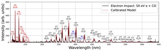
Comparison of the theoretical model and electron impact spectrum produced by 50 eV electrons incident on CO gas. For the Comet Tail (CT; black) and Baldet–Johnson (BJ; blue) systems, tick marks indicate the red and blue branches of each band and labels show the associated upper (|$v^{\prime }$|) and lower |$(v^{\prime \prime })$| vibrational numbers in the form |$(v^{\prime },v^{\prime \prime })$|. First Negative (FN; B|$^2\Sigma$|-X|$^2\Sigma$|) labels are shown in red. The spectrum is generated from the re-calibrated transition rates and derived vibrational populations. Equal populations in the red and blue branches of each band, and a rotational temperature of 300K, measured from a fit to the (3,0) band, is assumed. The ratio of A|$^2\Pi$|:B|$^2\Sigma$| population is approximately 315:1. Losses due to optical elements and travel outside the field of view are taken into account.
Transition rates pre- and post-calibration are provided in Supplementary Files, with additional details regarding how each band was calibrated.
