


ABSTRACT
We use the voids-within-voids-within-voids (VVV) simulations, a suite of successive nested N-body simulations with extremely high resolution (denoted, from low to high resolution, by L0 to L7), to test the Press–Schechter (PS), Sheth–Tormen (ST), and extended Press–Schechter (EPS) formulae for the halo abundance over the entire mass range, from minihaloes of 10−6 M⊙, to cluster haloes of 1015 M⊙, at different redshifts, from z = 30 to the present. We find that at z = 0 and z = 2, ST best reproduces the results of L0, which has the mean cosmic density (overdensity δ = 0), at 1011−15 M⊙. The higher resolution levels (L1–L7) are biased underdense regions (δ < −0.6). The EPS formalism takes this into account since it gives the mass function of a region conditioned, in this case, on having a given underdensity. EPS provides good matches to these higher levels, with deviations ≲20 per cent, at 10−6−12.5 M⊙. At z ∼ 7−15, the ST predictions for L0 and the EPS for L1–L7 show somewhat larger deviations from the simulation results. However, at even higher redshifts, z ∼ 30, EPS fits the simulations well again. We confirm our results by picking more subvolumes from the L0 simulation, finding that our conclusions depend only weakly on the size and overdensity of the region. The good agreement of EPS with the higher level simulations implies that PS (or ST) gives an accurate description of the total halo mass function in representative regions of the universe.
1 INTRODUCTION
In the Lambda cold dark matter (ΛCDM) model structures grow hierarchically from primordial quantum fluctuations to the galactic haloes and large-scale structures in the universe observed today (Davis et al. 1985). The abundance of these structures as a function of their mass provides a fundamental basis for galaxy formation models (White & Frenk 1991) and a framework for constraining cosmological parameters (Frenk et al. 1990; White, Efstathiou & Frenk 1993; Henry et al. 2009; Allen, Evrard & Mantz 2011). It is important, therefore, to develop theoretical models that describe how initial density perturbations collapse into non-linear structures, and to use these as tools for interpreting the predictions of N-body simulations.
Using the statistics of Gaussian random fields and the spherical collapse model, Press & Schechter (1974) proposed the well-known analytical model for halo mass functions, the so-called Press–Schechter formalism (PS model hereafter), which, at least qualitatively, predicts halo abundances that are comparable to numerical simulations. However, the PS model overpredicts the halo mass function in the low-mass regime (by even up to 60 per cent at z = 0) and exhibits too sharp a decrease at the high-mass end (White, Efstathiou & Frenk 1993; Gross et al. 1998; Governato et al. 1999; Jenkins et al. 2001; Lukić et al. 2007; Pillepich, Porciani & Hahn 2010). To remedy this, Sheth & Tormen (1999, 2002) replaced the spherical collapse ansatz in the PS model with the ellipsoidal collapse model and provided another formula (ST model hereafter) whose predictions provide a somewhat closer match to those of numerical simulations. For example according to Reed et al. (2003), the difference between the ST halo mass function and their simulated one is ≲10 per cent in well-sampled mass bins.
Bond et al. (1991), Bower (1991), and Lacey & Cole (1993) extended the PS model (hereafter the EPS model), to include predictions for the halo abundance and assembly history in different environments (Gao et al. 2005; Faltenbacher, Finoguenov & Drory 2010). Thereafter, several studies have attempted to provide accurate and universal fitting formulae for halo mass functions from numerical simulations (e.g. Jenkins et al. 2001; Warren et al. 2006; Lukić et al. 2007; Reed et al. 2007; Tinker et al. 2008; Crocce et al. 2010; Manera, Sheth & Scoccimarro 2010; Watson et al. 2013; Despali et al. 2016), improving upon earlier fits by extending to higher redshifts and wider mass ranges, and also considering different definitions of halo mass.
It is challenging to perform cosmological simulations with high mass resolution over a wide mass range down to redshift z = 0 because of computational cost. Previous studies, therefore, have focused primarily on either high-mass haloes (1010−15 M⊙) down to low redshift (e.g. Jenkins et al. 2001; Tinker et al. 2008) or low-mass haloes (105−10 M⊙) at high redshifts (e.g. z = 10, 30, see Lukić et al. 2007; Reed et al. 2007). As a result, there are comparatively few studies comparing the theoretical halo mass functions (e.g. the PS, ST, and EPS models) to simulations at the mass range of minihaloes (≲105 M⊙) down to low redshift (Angulo et al. 2017). Furthermore, most comparisons of EPS predictions with simulations focus on overdense or mean density regions. In this work, we use the voids-within-voids-within-voids (VVV) simulations (Wang et al. 2020), a series of successive nested zoom cosmological simulations of void regions with extremely high mass resolution, to test the accuracy of theoretical halo mass functions over the full mass range of CDM haloes as a function of time. By construction, this work focuses on the abundance of haloes in preferentially underdense regions.
The paper is organized as follows. Section 2 briefly describes the PS, ST, and EPS theoretical halo mass functions and Section 3 the details of our simulations. Our results, discussions, and conclusions are presented in Sections 4, 5, and 6, respectively. An examination of the conversion between linear and non-linear overdensities are illustrated in Appendix A. Further tests with the EAGLE simulations (Evolution and Assembly of GaLaxies and their Environments, Schaye et al. 2015) are presented in Appendix B.
2 THEORETICAL HALO MASS FUNCTIONS
Press–Schechter theory (Press & Schechter 1974) assumes that the initial density field follows a Gaussian random distribution, and that gravitational collapse occurs when the smoothed density field, δ, exceeds the critical overdensity for collapse, δc, during its random walk in the space of σ(M) − δ, where σ(M) represents the variance of the density field smoothed with a filter of mass, M, by the conventional real-space top-hat filter (e.g. Lacey & Cole 1993; Mo & White 2002). These crossing events correspond to structure formation on a certain scale, yielding a halo mass function given by
where |$\bar{\rho }_0 = \Omega _\mathrm{m}\rho _{\mathrm{crit,}z\mathrm{=0}}$| is the mean matter density, ν(M, z) = δc/[D(z)σ(M)], δc = 1.68647, and D(z) is the growth factor given by D(z) = g(z)/[g(0)(1 + z)], with (assuming a flat universe, i.e. |$\Omega _\mathrm{m} + \Omega _\Lambda = 1$|)
and a is the scale factor defined as (1 + z)−1.
While PS theory considers a spherical model for the collapse of perturbations, the ST (Sheth & Tormen 1999, 2002) model takes ellipsoidal collapse1 into consideration, leading to a modified formula:
where |$\nu ^{\prime }=\sqrt{a_\mathrm{ST}} \nu$|, with free parameters aST = 0.707, AST = 0.322, and qST = 0.3.
EPS theory (Bond et al. 1991; Lacey & Cole 1993; Mo & White 1996) is a useful tool to quantify halo assembly history and assembly bias. In particular, it predicts the probability that matter in a spherical region of mass, M0, at redshift, z0, and linear overdensity, δ0, is contained within dark matter haloes of mass in the interval (M1, M1 + dM1) at redshift z1
where, for a virialized structure, δ1 = δc/D(z), and δ0 is given by2
as an approximate solution of equations (16)–(17) of Mo & White (1996). Equation (6) is just an approximation to the exact solution that relates the non-linear density to the linear density during the collapse of a homogeneous sphere. Here, δnl denotes the non-linear overdensity in Eulerian space, which can be calculated directly from an N-body simulation. We modified the original formula from Mo & White (1996) and Sheth & Tormen (2002) by including an additional factor, C(δnl), to improve the accuracy of the fit when the non-linear overdensity is close to −1. We carried out our own fit to the spherical collapse model and obtained a correction factor of C(δnl) = 1 − 0.0053977x + 0.00184835x2 + 0.00011834x3 with x = min(0, ln (1 + δnl)). This makes a difference of about 5 per cent for δnl = −0.99.
Once these are calculated, we may obtain the corresponding halo mass function as
where a factor of (1 + δnl) is introduced to accommodate the difference of the sphere sizes in Eulerian and Lagrangian space. It is worth noting that, in the limit where the density of a large region is equal to the cosmic mean matter density (i.e. δnl = 0), the EPS formula reverts to the standard PS formula.
3 DETAILS OF THE SIMULATIONS
We use the nested zoom N-body simulations of the VVV project (Wang et al. 2020), which consists of eight levels of resimulation, covering a wide halo mass range spanning around 20 orders of magnitude (∼10−6−1015 M⊙). These simulations were performed with the gadget-4 code (Springel et al. 2021), adopting cosmological parameters derived from Planck (Planck Collaboration 2014): Ωm = 0.307, ΩΛ = 0.693, h = 0.6777, ns = 0.961, and σ8 = 0.829. On large scales (k ≤ 7 Mpc−1), the initial linear power spectrum is computed with the camb code (Lewis, Challinor & Lasenby 2000), while the BBKS fitting formula (the Bardeen-Bond-Kaiser-Szalay formula, Bardeen et al. 1986) with Γ = 0.1673 and σ8 = 0.8811 is adopted to extrapolate the power spectrum to small scales (k ≥ 70 Mpc−1), with a smooth transition between 7−70 Mpc−1.
In the VVV, we select candidate resimulation regions to be nearly spherical in shape and underdense (relative to the cosmic mean density); initial conditions for these candidate regions are then generated at higher resolution for each subsequent VVV resolution level. This nested zoom technique is ideal to study extremely small structures embedded within cosmologically representative environments (Jenkins 2010, 2013; Jenkins & Booth 2013). We refer the reader to Wang et al. (2020) for a detailed description of the zoom-in strategy. Wang et al. (2020) present eight levels of resolution with uncut initial power spectra,3 labelled L0–L7. L0 refers to the periodic, ‘parent’ simulation cube with Lbox = 738 Mpc. Following Wang et al. (2020), in L1–L7 we only consider the halo population contained within 0.8 times the radius of the high-resolution region, so as to avoid any potential contamination from low-resolution particles in the boundaries of the high-resolution regions. Details of the simulations at each resolution level are given in Table 1.
Properties of the different resolution levels in the VVV simulation used in this work. Column 1: name of the level; column 2: size (Lbox or dsphere) of the region selected at each resolution level at z = 0 – we use the entire cube in L0, while in L1–L7, we use the central sphere of diameter ∼0.8 times the diameter of entire high-resolution region; column 3: mass of high-resolution particles; column 4: softening length of high-resolution particles; column 5: overdensity (|$\delta _\mathrm{level} = \bar{\rho }_\mathrm{level} / \rho _{\mathrm{m}}-1$|) of the selected region at z = 0.
| Level | Size (Mpc) | mp (M⊙) | ϵ (kpc) | δlevel (z = 0) |
|---|---|---|---|---|
| L0 | 7.38 × 10² | 1.56 × 10⁹ | 6.83 | 0.0 |
| L1 | 8.12 × 101 | 7.41 × 10⁵ | 5.31 × 10⁻¹ | −0.607 |
| L2 | 1.23 × 101 | 1.45 × 10³ | 5.61 × 10⁻² | −0.918 |
| L3 | 1.65 | 2.82 | 8.32 × 10⁻³ | −0.964 |
| L4 | 2.22 × 10⁻¹ | 5.50 × 10⁻³ | 1.04 × 10⁻³ | −0.974 |
| L5 | 4.55 × 10⁻² | 5.75 × 10⁻⁵ | 2.27 × 10⁻⁴ | −0.976 |
| L6 | 9.43 × 10⁻³ | 2.60 × 10⁻⁷ | 3.77 × 10⁻⁵ | −0.986 |
| L7 | 1.58 × 10⁻³ | 8.55 × 10⁻¹⁰ | 5.28 × 10⁻⁶ | −0.984 |
Haloes were identified using a friends-of-friends (FOF) algorithm (Davis et al. 1985, assuming a linking length, b = 0.2 times the mean interparticle separation). Subhaloes within haloes were identified using the subfind algorithm (Springel et al. 2001; Dolag et al. 2009); both methods are built into gadget-4. There are many different definitions of halo mass: a basic approach is to adopt the mass of the FOF group (MFOF) directly, while others may use MΔ, defined as the mass-scale within which the average density is equal to Δ times the critical or the mean density of the universe. The overdensity, Δ, may be set in various ways, e.g. 200, 200Ωm, or Δν from the spherical top-hat collapse model (Eke, Cole & Frenk 1996; Bryan & Norman 1998). There is no consensus as to which definition is ‘best’. Warren et al. (2006) argued that the FOF mass could suffer from a systematic bias for haloes with small particle numbers, while Tinker et al. (2008) calibrated the parameters in a fitting formula with different mass definitions. In this paper, we adopt |$M_{\Delta =200\Omega _\mathrm{m}}$| (M200 hereafter), as the definition of halo mass. We consider only central haloes (excluding subhaloes) in the following analysis.
4 RESULTS
4.1 Halo mass function at z = 0
We begin by considering the halo mass function at z = 0, shown in Fig. 1, for each of the different resolution levels (L0–L7, solid lines of different colours). We only include haloes containing at least 50 particles. We compare with the corresponding EPS prediction (dashed colour lines) based on the local overdensity and total mass of each high resolution region. Error bars in the halo mass function are Poisson errors measured in each mass bin; these are usually largest at the high mass end because of the small number of high-mass haloes at each resimulation level (e.g. only 18 for the largest mass bin of L0).
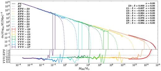
Predicted and simulated halo mass functions in different resolution levels at z = 0. In the top panel, the colour solid lines show the halo mass functions in the VVV (error bars represent Poisson errors); black, grey, and colour dashed lines show predictions of the PS, ST, and EPS models for each resolution level, respectively. In the bottom panel, the solid lines show the ratio VVV/EPS. Thick lines indicate mass bins containing at least 20 haloes. The black dotted line represents a ratio of unity, while the grey dashed line represents the ratio ST/PS. At z = 0, ST gives the best prediction for L0; EPS overpredicts the halo abundance in higher resolution levels by ∼20 per cent.
It can be seen that at z = 0, EPS gives relatively more precise predictions for the results of the simulations (within ∼20 per cent) at all resolution levels compared to PS (black dashed line). This is especially true at the higher levels (i.e. lower underdensity regions). ST (grey dashed line) gives the best prediction at L0 (only at cosmic mean density), resulting in the similarity between VVV/EPS (i.e. the ratio between the simulation halo mass function and the EPS prediction), and ST/PS (i.e. the ratio between the ST and PS halo mass functions, grey dashed line truncated at 50 mp, L0 in the bottom panel) lines for L0.
Our results from PS and ST for L0 at z = 0 agree with previous studies (e.g. Jenkins et al. 2001; Reed et al. 2003, 2007; Yahagi, Nagashima & Yoshii 2004; Lukić et al. 2007; Pillepich, Porciani & Hahn 2010), suggesting that the ST model is a better approximation than PS for volumes simulated at mean density and low redshift. This is true even when we use M200 rather than MFOF as the definition of halo mass. For example Reed et al. (2003) studied the halo mass function in the mass range ∼1010.2−1014.2 M⊙4 and found that PS overpredicts the abundance by around 20 per cent when M < 1013.7 M⊙ at z = 0; ST, on the other hand, performs comparatively better in the same mass range – this is consistent with our findings that the halo mass function of L0 at the low mass end (M ≲ 1014 M⊙) aligns with the ST prediction and is ∼20 per cent lower than PS prediction. On the other hand, it is worth noting that while the simulated halo mass function tracks the ST prediction well at the high mass end, the PS model underpredicts the halo mass function of L0 at M ≳ 5 × 10¹⁴ M⊙. This is also consistent with the results of White, Efstathiou & Frenk (1993), Gross et al. (1998), Governato et al. (1999), Jenkins et al. (2001), Lukić et al. (2007), and Pillepich, Porciani & Hahn (2010).
In the higher resolution level simulations (L1–L7, corresponding to increasingly underdense regions), the EPS model performs significantly better than either PS or ST. A simple comparison can be made with the halo mass function at the high mass end of the L1 volume in Fig. 1 – even with the most moderate underdensity (δ = −0.607), both PS and ST significantly overpredict the halo abundance, while EPS provides a relatively accurate prediction. This is to be expected because these simulations focus on regions far below the average density of the universe. Indeed, it is known that the halo mass function depends strongly on local overdensity (Gao et al. 2005; Rubiño-Martín, Betancort-Rijo & Patiri 2008; Crain et al. 2009; Faltenbacher, Finoguenov & Drory 2010; Tramonte et al. 2017). For example Gao et al. (2005) find that at z = 49, the halo mass function in a region with δnl = 4.3 has a larger amplitude than that in a region with δnl = 2.8 by a factor of ∼4. Only the EPS model takes local environment into consideration when predicting the abundance of haloes. The mass function of L6 (blue line) is less aligned with other levels. This may be due to cosmic variance (i.e. the scatter in halo abundance across volumes of the same size and matter density; we refer readers to Section 4.3 for a detailed illustration). We examine this by comparing the halo mass function in L6 and the corresponding volume in L5 (ensuring the same non-linear overdensity) and find good agreement, which excludes the possibility of problems related to numerical convergence in L6. In general, EPS provides reasonably accurate predictions (particularly at the low-mass end) which overestimate our simulated halo mass functions by ∼20 per cent. This might be due to various reasons, e.g. the ambiguous definition of a ‘virialized’ halo in the original PS theory.
4.2 The redshift evolution of the halo mass function
After examining the accuracy of theoretical predictions of the halo mass function at z = 0, we now consider how well these models perform at higher redshift. In Fig. 2, we show the halo mass functions at redshifts ∼ 2, 7.8, and 30. For L0, at low redshift, the simulation result is in good agreement with the ST prediction. With increasing redshift, however, better agreement is gradually found with the PS and EPS models (the PS and EPS predictions are rather similar when δ = 0 and the enclosed mass is large enough).
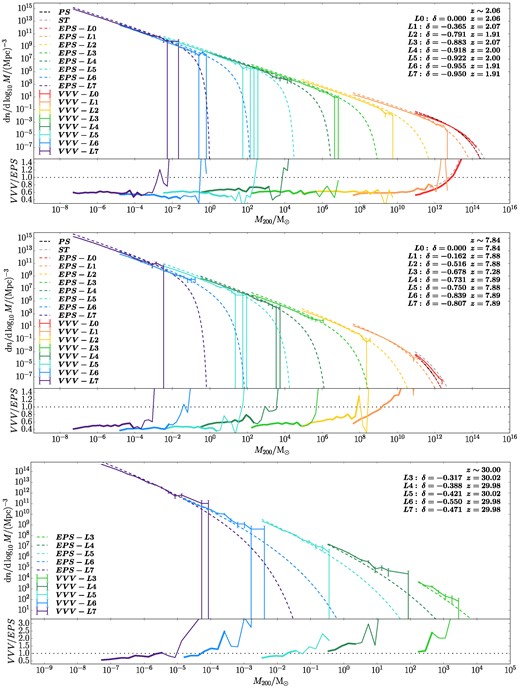
As Fig. 1, but for z ∼ 2 (top panel), z ∼ 7.8 (middle panel), and z ∼ 30 (bottom panel). For z ∼ 30, we only show results from L3–L7 as very few haloes have formed at this time in the lower resolution levels. The PS and ST predictions are calculated at the corresponding redshifts, while the simulation results and the EPS predictions are shown at the closest available redshift output in the simulation. At higher redshifts, the EPS prediction deviates more from the simulations, by ∼20–50 per cent, especially at z ∼ 7.8.
Our results at z ≲ 2 are consistent with many previous studies (Reed et al. 2003; Yahagi, Nagashima & Yoshii 2004; Lukić et al. 2007; Klypin, Trujillo-Gomez & Primack 2011), which find that the ST model is a good fit at low redshift. However, as redshift increases, there are discrepancies among these simulation studies: Reed et al. (2003) (∼1010.2−12.2 M⊙), Lukić et al. (2007) (∼108.2−10.2 M⊙), and Wang, Gao & Meng (2022) (∼108.2−11.2 M⊙) suggested that the deviation of ST from the simulation data (using MFOF as the halo mass) is ≲15 per cent at z ≲ 10. On the other hand, Hellwing et al. (2016; also using MFOF) showed that ST significantly overpredicts the halo abundance at 0.5 ≤ z ≤ 5, eventually becoming a better approximation at z ∼ 9.
Cohn & White (2008) discussed the differences arising from using different definitions of halo mass at z = 10: the halo mass function with MFOF in the mass bin 108.2−10.7 M⊙ agrees with the ST prediction at z = 10, while its counterpart with M180 is almost half of the MFOF measurement. Klypin, Trujillo-Gomez & Primack (2011) (using |$M_{\Delta _\nu }$|, with Δν the value from the spherical top-hat collapse model) found that the deviation between ST and the simulations becomes larger at higher redshift – up to a factor of 10 in mass bin 1010.2−11.2 M⊙ at z = 10. When using a similar definition of halo mass, our results agree with the last two studies, suggesting that the halo mass function with mass defined as M200 is lower than the ST prediction and approaches the PS or EPS prediction at high redshift.5 We note that, when defined using MFOF, the halo mass function (not shown) of L0 deviates less from the ST prediction at high redshifts, which agrees with the conclusion of Reed et al. (2003) that the halo mass function obtained using spherical overdensity masses is lower than the mass function based on the FOF mass.
For the higher VVV resolution levels, the results at z ∼ 2 are quite similar to the results at z = 0: the halo mass functions in the simulations are still in fairly good agreement with the EPS prediction. On the other hand, at z ∼ 7.84 the difference between the simulations and the EPS prediction becomes larger, with the ratio of VVV/EPS dropping to ∼50 per cent for L2–L7. At z = 30 results from L3–L7 show that the low-mass end of the halo mass function (computed so that haloes contain at least 50 particles and each bin contains at least 20 halo samples) goes back to being aligned with EPS.
In Fig. 3, we plot the evolution of the geometric mean of the ratio VVV/EPS6 in each resolution level. Error bars have been propagated from the Poisson errors of selected mass bins using the following relations
where g and σg represent the value and the error of the geometric mean ratio respectively; x i and σi represent the value of the ratio and the Poisson error in the ith mass bin; and N is the number of mass bins.
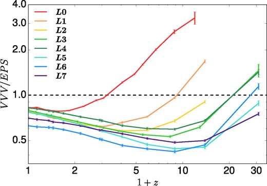
Evolution of the geometric mean of the ratio of the mass functions, VVV/EPS, in different resolution levels represented by the different colours. The error bars are the error of the mean value obtained by error propagation; see the main text for details. The deviations peak at z ∼ 2−9 (depending on scale), indicating that the EPS predictions fit the simulations best at low and extremely high redshifts.
Fig. 3 suggests that the ratios in all resolution levels follow similar tracks with time: the average VVV/EPS ratios are close to one at the present, drop at intermediate redshifts, and increase again at earlier times. Generally, the higher the level is, the earlier their track intersects the dashed horizontal line at unity, which is likely related to the different characteristic mass scales of haloes in each level.
We find that the average VVV/EPS ratios are close to unity at low redshifts for large masses and, at high redshifts, for low masses. This is consistent with the results of Gao et al. (2005), who studied the halo mass function in denser environments at z = 0 and z = 49, and showed that EPS gives accurate predictions in the mass ranges 108.2−10.7 M⊙ (z = 0), and 102.7−5.2 M⊙ (z = 49), confirming that EPS is a good fit at low redshift and extremely high redshift.
4.3 Halo mass functions with different realizations
The analyses in the preceding section use only one realization for each resolution level and are thus subject to ‘cosmic variance’. To assess the effect of this variance and test the accuracy of the theoretical models of the halo mass function in general, we picked spherical regions of different sizes and overdensities from the L0 cube, and measured the average halo mass function in them. The L0 volume is large enough to sample a range of overdensities with statistical fidelity. We generated 105 randomly located points and measured their local overdensities inside spheres of different radii, and then selected 100 samples with the closest overdensity to a set of preselected values. We then computed the mean halo mass function across these 100 samples; this is displayed in Fig. 4. Black (grey or coloured) dashed lines represent the predictions of PS (ST or EPS), and the colour solid lines show the mean halo mass function of samples in the VVV simulation. Different colours represent different overdensities, the values of which are adapted to the redshift and sphere size of each panel (marked at the upper right corner), in order to obtain a large enough sample.
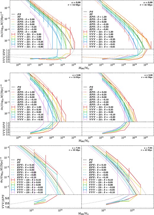
Average halo mass function in spherical regions of different overdensity selected from the L0 cube. The left and right columns correspond to different region sizes; each row corresponds to a different redshift (increasing from top to bottom). Black, grey, and colour dashed lines show the PS, ST, and EPS predictions, respectively; the colour solid lines show the simulation results, with different colours corresponding to different overdensities. The error bars represent the 16–84th range amongst the regions; the orange dash–dotted line in the upper right panel shows the VVV L1 simulation with Poisson errors. The halo mass functions of the different realizations are generally consistent with those obtained from the full simulation.
It can be seen that the ratio VVV/EPS (for M200) depends only weakly on sphere size and overdensity, but evolves with redshift – it agrees with the theoretical ST/PS line at z = 0 and 2, but deviates at z = 7.84. The mean halo mass function averaged over the random samples is quite similar to that of the full volume, corroborating our conclusion from the full simulation that the ST model provides a good approximation to the halo mass function at low redshifts, but overpredicts it at high redshifts. However, the size of the error bars suggests that even for regions with the same overdensity and total mass, there is considerable variance in the halo mass function. This is especially true in smaller regions and might be part of the reason why the predicted halo abundance in some levels (e.g. L6) are less accurate compared to other levels. In the upper right panel of Fig. 4, we also show the halo mass function of L1 at z = 0 (r = 41 Mpc, δ = −0.61) with an orange dash–dotted line. Comparing to its counterpart in L0 (purple solid line), we find that the L1 mass function is a little larger, by |$\lesssim 10~{{\ \rm per\ cent}}$|, at M200 ∼ 1012.5 M⊙, showing reasonable convergence in the halo mass function between the two different levels.
5 DISCUSSION
In the previous section, we have shown that for different subvolumes of the L0 simulation (corresponding to regions with a range of overdensities), the halo abundance in the EPS model differs from the halo abundance in the simulation at a similar level (20–40 per cent at z = 0, higher at high z) as in the L0 full volume, which has cosmic mean density. We expect this conclusion to hold not just for a relatively small range in halo mass, but also for smaller masses, down to the cut-off in the power spectrum; we are unable to perform similar tests for higher levels due to the limited sample size in zoomed regions. Consequently, the deviations between the EPS predictions and the (L1–L7) VVV simulations (Figs 1 and 2) should approximately reflect the difference at other overdensities, rather than just the underdense regions probed by the VVV simulations. Combining these two arguments, given that the PS formalism is equivalent to integrating the EPS formula over all linear overdensities, δ0, we can use the PS formula to predict the abundance of haloes across the entire range of halo masses at the mean density.
Based on this, in Fig. 5, we present the evolution of halo abundance in the whole universe (at mean density) as predicted by the PS (black) and ST (coral) formalisms. The predictions are similar to those of Mo & White (2002), but we show the differential mass function, and display it over a much more extended mass range than Mo & White (2002) and with updated cosmological parameters. The comparison with the halo mass function in the L0 simulation (red lines) corroborates our previous results that, at low redshift (z ≲ 2) and high masses (1011−15 M⊙), the ST model provides a better prediction, while the PS model underpredicts the abundance of large haloes (≳1015 M⊙) and overpredicts the abundance of smaller haloes (∼1011−14 M⊙). At higher redshifts, the simulation results lie between the PS and ST predictions.
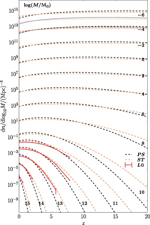
The evolution of halo abundance within the mass range 10−6–1015 M⊙ in the whole universe (or mean density regions) predicted by PS (black lines) and ST (coral lines), with the numbers beside each line representing the corresponding log (M/M⊙). The dashed lines show the prediction with the uncut initial power spectrum, while the dotted lines take account of the free-streaming effect at 10−6–10−4 M⊙. The red lines are the halo mass function in the L0 simulation, with the error bars representing Poisson errors. Within the mass range 1011–1015 M⊙, ST is a good approximation at low redshift z ≲ 2, but overpredicts the halo number density at earlier times. The free-streaming effect suppresses the abundance of 10−6 M⊙ haloes by approximately one order of magnitude, while barely affecting larger haloes.
For the two lowest mass bins (i.e. 10−6 M⊙ and 10−4 M⊙), we show the effect of the free-streaming cut-off for the 100 GeV neutralino with dotted lines, using the cut-off initial power spectrum of Wang et al. (2020). Note that here we have used the sharp k-space window function to evaluate σ(M) in the theoretical mass functions, as suggested by Benson et al. (2013). This modification provides a more accurate prediction of the halo abundance near the cut-off scale compared to a real-space top-hat filter, which instead overpredicts the mass function near the cut-off by re-weighting long wavelength modes. We find that the effect of free-streaming is to suppress the abundance of 10−6 M⊙ haloes by one order-of-magnitude, while larger haloes are barely affected.7 This is consistent with previous studies of warm dark matter models (e.g. Schneider et al. 2012; Benson et al. 2013; Bose et al. 2016), which suggest that free-streaming only suppresses the halo mass function near and below the cut-off scale.
6 SUMMARY AND CONCLUSIONS
In this paper, we have made use of the VVV simulations, a suite of multizoom nested simulations at very high resolution, to test the accuracy of the PS, ST, and extended EPS models for the abundance of haloes as a function of their mass and redshift. In particular, this work focuses on the halo mass function at extremely small-scales (down to ∼10−6 M⊙) and its evolution to high redshift (z = 30). The resolution levels are labelled L0–L7, corresponding to smaller, higher density regions of progressively higher mean underdensity (below the cosmic mean). The non-linear underdensity of each level is mapped into a linear underdensity using fitting formulas from the EPS formalism.
We find that at z = 0, the ST model provides the most accurate fit to the halo mass function in the L0 volume (overdensity, δ = 0; 1011−15 M⊙) but the EPS model provides the best fit to the higher resolution levels (L1–L7; δ < −0.6 at 10−6−12.5 M⊙), to better than 20 per cent accuracy (see Fig. 1). The results at z = 2 are similar, but there are larger deviations at z ∼ 7−15 from the ST prediction in L0 and from the EPS predictions in the higher resolution levels. However, at even higher redshift, z ∼ 30 (10−6−2.5 M⊙; −0.55 < δ < −0.30), the EPS model provides, once more, a good fit to the halo mass functions in the simulations (see Figs 2 and 3). We validated our results by selecting regions of different volume and overdensity from the full L0 volume, and find that the VVV/EPS ratio (for M200) depends only weakly on region size and overdensity, but increasingly deviates from unity at higher redshifts (Fig. 4). Finally, we tested convergence by comparing the halo mass function in L1 with those in selected subvolumes of L0 spanning a range of sizes and overdensity.
Having demonstrated that the EPS formalism gives a good description of the halo mass function in the biased regions of the VVV high resolution levels, given the arguments in Section 5, it is reasonable to assume that the PS formalism (or the ST formula) also gives a good description of the halo mass function in representative, mean density regions. Thus, we are able to present the actual halo mass function (number of haloes per unit volume) over the entire mass range in ΛCDM, from 10−6 to 1015 M⊙ (Fig. 5). While the mass function at the high mass end is, of course, well-known, our study is the first to explore the minihalo regime (≲105 M⊙) where the EPS model provides a prediction for the halo mass function, with deviations at the ∼20–50 per cent level, which could be reduced with further theoretical work. Finally, we note that since we have analysed dark matter only simulations, the impact of baryons on the haloes is ignored. A more complete study based on hydrodynamics simulations with full baryon physics will be presented in a forthcoming paper.
ACKNOWLEDGEMENTS
We thank the anonymous referee for a constructive report that helped us tighten up our analytical arguments and improve our manuscript. We would like to thank Simon D. M. White, Volker Springel, and Shaun Cole for useful discussions and advice. We acknowledge support from the National Natural Science Foundation of China (Grant Nos. 11988101, 11903043, 12073002, and 11721303) and the K. C. Wong Education Foundation. HZ acknowledges support from the China Scholarships Council (No. 202104910325). SB is supported by the UK Research and Innovation (UKRI) Future Leaders Fellowship (grant number MR/V023381/1). CSF acknowledges support by the European Research Council (ERC) through Advanced Investigator grant, DMIDAS (GA 786910). JW acknowledges the support of the research grants from the Ministry of Science and Technology of the People’s Republic of China (No. 2022YFA1602901), the China Manned Space Project (No. CMS-CSST-2021-B02), and the CAS Project for Young Scientists in Basic Research (Grant No. YSBR-062). This work used the DiRAC@Durham facility managed by the Institute for Computational Cosmology on behalf of the STFC DiRAC HPC Facility (www.dirac.ac.uk). The equipment was funded by BEIS capital funding via STFC capital grants ST/K00042X/1, ST/P002293/1, ST/R002371/1, and ST/S002502/1, Durham University and STFC operations grant ST/R000832/1. DiRAC is part of the UK National e-Infrastructure.
DATA AVAILABILITY
The data used in this paper will be shared upon reasonable request to the corresponding author.
Footnotes
The spherical collapse model considers the evolution of a spherically symmetric density perturbation; the ellipsoidal model makes the more realistic assumption that the overdense region is an ellipsoid, which leads to different collapse times in different directions.
The accuracy of this formula in underdense regions is examined in Appendix A.
There are two additional levels (L7c and L8c) where the initial power spectrum is cut-off on small-scales to reflect the free-streaming of a 100 GeV neutralino. Simulations where this free-streaming cut-off is resolved are known to produce spurious structures (e.g. Wang & White 2007; Lovell et al. 2014). Thus, for simplicity, we exclude these two levels from our analysis.
We convert the mass unit of the works referred in this paper from h−1M⊙ to M⊙ for easy comparison.
As shown in Appendix B, we corroborate our results with the EAGLE dark matter only simulations.
We only use haloes with at least 50 particles and mass bins with at least 20 samples. We checked that our results are independent of bin size and the precise threshold number of samples in each bin.
We also compared the predictions with the same sharp k-space filter, but different initial power spectra, and confirmed that the suppression comes from the free-streaming effect.
This method neglects the edges between the particle spheres and the boundary of the region, but since the particle number is large enough, it only overestimates the density by |$\lesssim 3~{{\ \rm per\ cent}}$|.
It is worth noting that at such high redshift (z = 31.39), δ0 is very close to δnl for most regions as structures have not yet formed and δnl(z = 31.39) ∼ 0. However, the difference increases as δ0 → −∞ with δnl → −1 according to the formula.
References
APPENDIX A: CONVERSION BETWEEN LINEAR AND NON-LINEAR OVERDENSITY
We converted the non-linear overdensity measured in the simulation to a linear overdensity using equation (6), as required by the EPS theory. Here, we examine whether this fitting formula is still accurate for the extremely underdense regions of interest in VVV. We generated 104 random positions in the VVV–L0 volume at z = 0, and measured the non-linear overdensities, δnl(z = 0), within spheres of radius r = 15 Mpc, each of which would contain ∼106 particles if δnl = 0. For each sphere, we then traced the contained particles back to z = 31.39. We then constructed the polyhedron with the smallest volume containing all these particles. The polyhedron was used to estimate the non-linear overdensity, δnl(z = 31.39).8 We tested equation (6) by converting the two measured non-linear overdensities into linear overdensities9 and comparing them.
We note that it is very likely for the polyhedron at z = 31.39 to contain particles that no longer belong to the corresponding sphere at z = 0. To account for this, we define ftraced as the fraction of particles that are traced from z = 0 to the polyhedron, describing the extent to which the measurement of the overdensity in this volume is uncontaminated by other particles. In other words, a low value of ftraced means that the polyhedron at z = 31.39 contains a small fraction of particles that eventually end up in the corresponding sphere at z = 0.
In Fig. A1, we plot the linear overdensity at z = 31.39 against the non-linear overdensity at z = 0. The bottom panel shows the ratio between the difference and the predicted value. The purple line, representing the median value for all samples (including those highly contaminated volumes with low ftraced), deviates most from the black dashed line, which is the prediction from equation (6). The red and orange lines are restricted in ftraced (indicating uncontaminated volumes); these predictions are well aligned with the results in simulation. The largest values of |Δδ0/δ0| occur near the middle of the range because δ0 itself is around zero as δnl ∼ 0. We also tested equation (6) with the correction function, C = 1, but the difference is negligible since the lowest non-linear overdensity here is only ∼−0.9 due to a lack of samples, where the Mo & White (1996) analytical fit and numerical solution are still very similar.
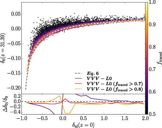
Conversion between non-linear and linear overdensities. The colour of each cross represents the fraction of traced particles in the volume at z = 31.39, indicating the extent to which the measurement of overdensity in that volume is contaminated by background particles; see the text for details. The purple solid line shows the median values for all samples and the red and orange lines the median values of samples with ftraced > 0.7 and 0.8, respectively. The black dashed line shows the prediction of equation (6). The bottom panel shows the ratio of the difference relative to the predicted value. Equation (6) provides a reasonably accurate fit to the simulations, especially for samples with high values of ftraced.
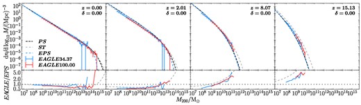
Comparison of the PS, ST, and EPS models with the halo mass functions measured in dark matter-only versions of the EAGLE simulation at different redshifts. The colour solid lines show the halo mass function in the EAGLE simulations of side Lbox = 34.37 Mpc (blue) and 100.00 Mpc (red); the error bars are Poisson errors. Black, grey, and colour lines show the predictions of the PS, ST, and EPS models. The EPS predictions were calculated for the entire mass in the EAGLE34.37 cube; for the larger total mass in the EAGLE100.00 box, the EPS predictions almost overlap with the PS model and are not shown for clarity. In the bottom panels, the colour solid lines show the ratio, EAGLE/EPS, while black dotted lines indicate a value if one; the grey dashed lines represent ST/PS. The results from the EAGLE simulations align well with our results from the VVV simulations.
APPENDIX B: TESTS IN FULL-BOX SIMULATIONS WITH HIGHER RESOLUTION
We also compared the predictions of the different models with the halo mass functions in dark matter-only versions of the EAGLE simulation (Schaye et al. 2015) with the same power spectrum but higher resolution than VVV–L0 (EAGLE34.37: Lbox = 34.37 Mpc, N = 10343, mdm = 1.44 × 10⁵ M⊙, and EAGLE100.00: Lbox = 100.00 Mpc, N = 15043, mp = 1.15 × 10⁷ M⊙). As shown in Fig. A2, the results are quite similar to those for VVV–L0: the ST model provides a good description of the halo mass functions in the simulations at low redshifts, but overestimates them at high redshifts (z ≳ 8), especially at the high mass end. Overall, the models provide reasonably accurate predictions that align with the results in the main text.
