


ABSTRACT
A less explored aspect of dwarf galaxies is their metallicity evolution. Generally, dwarfs have lower metallicities than Hubble sequence late-type galaxies, but in reality, dwarfs span a wide range of metallicities with several open questions regarding the formation and evolution of the lowest and the highest metallicity dwarfs. We present a catalogue of 3459 blue, nearby, star-forming dwarf galaxies extracted from SDSS DR-16 including calculation of their metallicities using the mean of several calibrators. To compile our catalogue we applied redshift, absolute magnitude, stellar mass, optical diameter, and line flux signal-to-noise criteria. This produced a catalogue from the upper end of the dwarf galaxy stellar mass range. Our catalogued dwarfs have blue g – i colours and Hβ equivalent widths, indicative of having undergone a recent episode of star formation, although their star formation rates (SFRs) suggest only a moderate to low enhancement in star formation, similar to the SFRs in low surface brightness and evolved tidal dwarfs. While the catalogued dwarfs cover a range of metallicities, their mean metallicity is ∼0.2 dex below solar metallicity, indicating relatively chemically evolved galaxies. The vast majority of the catalogue, with clean photometry, are relatively isolated dwarfs with only modest SFRs and a narrow range of g – i colour, consistent with internally driven episodic mild bursts of star formation. The presented catalogue’s robust metallicity estimates for nearby SDSS dwarf galaxies will help target future studies to understand the physical processes driving the metallicity evolution of dwarfs.
1 INTRODUCTION
Dwarf galaxies are overwhelmingly the most numerous type of galaxy in the Universe, but due to their low luminosity, only the most luminous are detectable beyond the local Universe (Dale et al. 2009; McConnachie 2012). Typically, dwarfs have much smaller optical diameters, 0.1 to 10 kpc (de Vaucouleurs et al. 1991), and stellar masses, 107 to 109 M⊙ (Lee et al. 2006), than the more massive galaxies in the Hubble sequence. Most dwarf galaxies also have a low oxygen abundance (12 + log(O/H) 7.0 to ≲ 8.4; e.g. Izotov & Thuan 1999; Kunth & Östlin 2000; Lee, Grebel & Hodge 2003).
Additionally, dwarf galaxies have been classified into several morphological subtypes, e.g. dwarf elliptical galaxies (dE), dwarf spheroidal galaxies (dSph), dwarf irregular galaxies (dIrr), dwarf spiral galaxies (dS), Magellanic type dwarfs (Sm, Im), blue compact dwarf (BCD) or HII (dwarf) galaxies, ultra-compact dwarf galaxies (UCD), and tidal dwarf galaxies (TDG), each with their characteristic properties (e.g. Sargent & Searle 1970; Grebel 2001; Pustilnik et al. 2001; Grebel, Gallagher & Harbeck 2003; Grebel 2004; Duc 2012; Lisker et al. 2013; Ahn et al. 2017; Janz et al. 2017).
There remain many unanswered questions about the origin and evolution of dwarf galaxies. For example, are the properties of the dwarf subtypes the result of different formation pathways or do they reflect different stages of a dwarf galaxy’s evolution?, e.g. Papaderos et al. (1996); van Zee, Skillman & Salzer (1998); Mayer et al. (2001); Sawala, Scannapieco & White (2012); Kim et al. (2020). While, for a few dwarf subgroups, e.g. TDGs, their origin and likely evolution are understood in outline at least (e.g. Duc et al. 1997; Braine et al. 2001; Duc 2012; Sengupta et al. 2013, 2015, 2017; Scott et al. 2018), for most dwarfs the physical processes driving their origin and relation to other dwarf types remain to be definitively established. Although, there are many studies which show correlations between dwarf properties (including kinematics, stellar populations, and morphologies) and their environments (e.g. Lisker et al. 2013; Sybilska et al. 2018; Toloba et al. 2018). An interesting aspect of dwarf galaxy evolution is their metallicity evolution, in particular the relationship between the mass of stars in a galaxy and its metallicity (e.g. Tremonti et al. 2004; Berg et al. 2012; Jimmy et al. 2015). Gas metallicity is the abundance of elements heavier than hydrogen and helium, so its value depends on the evolutionary state of the gas in the galaxies. A galaxy’s gas-phase metallicity, Z, can be represented by 12 + log(O/H), where the solar metallicity (Z⊙) is 12 + log(O/H)⊙ = 8.69 (Asplund et al. 2009). The lower metallicity of dwarfs is generally attributable to retarded star formation (SF) compared to more massive galaxies as a result of the downsizing phenomenon. There are, however, exceptions to the typical dwarf metallicity value, e.g. extremely metal-poor (XMP) dwarfs (12 + log(O/H) ≲ 7.65; Izotov & Thuan 2007; Papaderos et al. 2008; Lagos et al. 2014, 2016, 2018) and at the other extreme dwarfs with near solar oxygen abundances, e.g. TDGs (Duc & Mirabel 1999). It is still an open question whether the lowest metallicity dwarfs are survivors from the first epoch of galaxy formation or are young recently formed galaxies (e.g. Sargent & Searle 1970) or result from some other process such as metal-poor gas accretion (e.g. Lagos et al. 2016, 2018). To date, few studies of high metallicity dwarfs are available, and as a result, their formation scenarios are yet to be explored systematically. TDGs are known to be high-metallicity dwarfs, but not all high-metallicity dwarfs have been unambiguously found to have a tidal origin (Sweet et al. 2014).
While studies of the metallicity evolution in dwarf galaxies exist in the literature, they are either detailed, resolved studies of small samples (e.g. Lee et al. 2006; Lagos, Telles & Melnick 2007; Berg et al. 2012; Jimmy et al. 2015), or larger samples with additional selection criteria like a detected H i counterpart or limited range in metallicity (e.g. Jimmy et al. 2015; James et al. 2017) or higher redshift dominated samples (Tremonti et al. 2004; Peeples, Pogge & Stanek 2008; Li et al. 2023). An optically selected statistically large sample of low-redshift dwarf galaxies with robust metallicity estimates has not previously been available in the literature. This paper aims to fill that gap and presents a dwarf galaxy catalogue with metallicity estimates. The catalogue will facilitate the selection of subsamples for future multiwavelength follow-up or statistical studies to identify the physical processes driving the metallicity evolution in specific groups of dwarfs, especially for high-metallicity dwarfs.
We initially compiled a catalogue of undifferentiated dwarf galaxies from the Sloan Digital Sky Survey (SDSS) DR-16 (York et al. 2000). To quantify dwarf galaxy properties requires accurate redshifts. Therefore, we restricted our initial selection to galaxies with SDSS spectra, which allowed their redshifts to be determined accurately. Galaxies from this initial selection had the potential for other studies based on their spectra, e.g. determination of their metallicity, and SF history. But these types of study require galaxies which present strong emission lines. The final dwarf catalogue was restricted to dwarfs with sufficiently strong emission lines in their SDSS spectra to robustly determine their metallicities. Because of the selection criteria, the catalogue is not representative of dwarfs in general, but instead, it consists of the more massive star-forming, relatively high metallicity dwarfs in SDSS.
The layout of the paper is as follows. In Section 2, we discuss the methodology used to compile the catalogue. Section 3 presents the results obtained (e.g. metallicity estimates, star formation rate (SFR), and several other properties of the catalogue). Section 4 is a discussion on the scientific implications of the results and finally Section 5 summarizes the work carried out and the main results of the paper.
2 METHODOLOGIES
2.1 The sample
We started by selecting all DR-16 SDSS spectra within the radial velocity range of 500 |${\rm km}\, {\rm s}^{-1}$| ≤ v ≤ 10 000 |${\rm km}\, {\rm s}^{-1}$|, with a ‘GALAXY’ classification in ‘Class’, ‘Type’, and/or ‘SourceType’. This selection eliminated stars and quasars from our source list. The velocity range was chosen to avoid the difficulty of establishing distances to sources at velocities below 500 |${\rm km}\, {\rm s}^{-1}$| and the limited number of dwarfs with spectra in SDSS at velocities >10 000 |${\rm km}\, {\rm s}^{-1}$|. This upper limit is confirmed in Fig. 1, bottom right panel, where we see that the number of dwarfs in the catalogue falls rapidly towards the catalogue’s redshift upper limit.
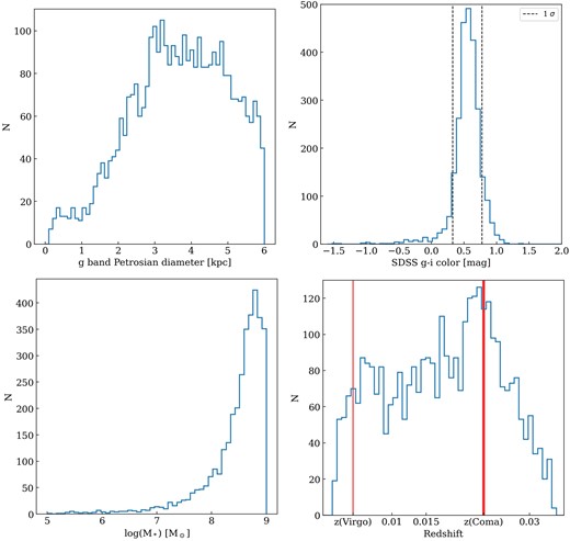
Histograms of selected properties of the catalogued dwarf galaxies: Top left: Dpet in kpc; top right: SDSS g − i colour; bottom left: log(M*/M⊙); bottom right: redshift, with the vertical red lines indicating the redshift and redshift uncertainties of the Virgo (z = 0.00436 ± 0.00002) and Coma (z = 0.02333 ± 0.00013) galaxy clusters.
To eliminate massive galaxies, all galaxies with an absolute g-band (∼4770 Å) magnitude, Mg ≤ −18 mag were excluded from our sample. Based on this selection of galaxies with absolute magnitudes ≥ −18 criteria, we obtained a preliminary catalogue containing 18 768 dwarf galaxy candidates. The next criterion applied was galaxy stellar mass. The stellar masses of the 18 768 galaxies were estimated using the relationship between the candidates’ photometric SDSS DR-16 model magnitudes for selected colour band filters and the stellar M/L ratio from Bell et al. (2003). The SDSS Pestrosian g-band luminosity (Lg) and g − r colour of the sources were used to calculate the stellar mass (M*) using equation (1):
For our dwarf catalogue, we chose only galaxies with stellar masses less than 109 M⊙, reducing the previous candidate list of 18 768 galaxies to 13 211. The above selection steps ensured that the catalogue contained only low stellar mass galaxies, but could not ensure that they were necessarily dwarf galaxies. To exclude galaxies with large optical diameters, such as low surface brightness (LSB) galaxies, we set an upper D25 limit of 10 kpc, approximately the diameter of the Large Magellanic Cloud (de Vaucouleurs et al. 1991). We calculated the relation between the SDSS Petrosian (Rpet × 2) diameter (Dpet) and the D25 isophotal diameter for a sample of the catalogue’s galaxies and found Dpet = 0.67D25 (D25 ∼ 1.5Dpet). Thus we used a g-band Dpet cut-off of 6 kpc, which is approximately equivalent to a D25 of ≤ 10 kpc. The sizes of the galaxies in kpc were obtained using the kpc/arcsec scale from the online Ned Wright Cosmology Calculator assuming H0 = 67.8 |${\rm km}\, {\rm s}^{-1}$| Mpc−1, ΩM = 0.308, and Ωvac = 0.692 (Wright 2006). The Dpet values in arcseconds were derived from SDSS. The catalogue of dwarf galaxies after applying the optical size cut-off contained 5683 sources. A further 55 candidates were removed from the catalogue as they displayed a clear spiral structure, inconsistent with them being dwarf galaxies. Amongst the remaining 5628 galaxies, 26 had multiple spectra for the same galaxy but from different projected positions. In these cases, we only retained the spectrum closest to the galaxy centre and thus our initial dwarf galaxy catalogue then contained 5602 candidates.
Having established an initial dwarf galaxy selection we further refined the catalogue by selecting only those dwarfs displaying strong emission lines in their SDSS spectrum which facilitated the study of their metallicity and SF histories. To do this, first, we removed the stellar component following the procedure explained in Section 2.2. Then we chose a subset of dwarfs based on the signal-to-noise ratio (SNR) of the spectral lines needed to determine their metallicities. To increase the robustness of the metallicity and other estimates (e.g. electron density), we only chose candidates with spectra where the emission lines used to determine these quantities (Hβ 4861Å, [O iii] 5007Å, Hα 6563Å, [N ii] 6584Å, [S ii] 6717Å, [S ii] 6731Å) all had an SNR ≥ 2.5. The SNR criterion was not applied to the weak [O iii] 4959Å and 4363Å lines, which were detected in only some galaxies. Applying this emission line SNR criterion reduced the number of galaxies in our final dwarf catalogue to 3459. Using the final 3459 galaxies, the four panels of Fig. 1 show the number distribution of the catalogue with respect to Petrosian diameter, g − i colour, log(M*/M⊙), and redshift.
2.2 Spectral fitting
Spectral synthesis is an important method to derive galaxy properties from their spectra. To fit the stellar component of our catalogued dwarfs, we used the spectral synthesis code Fitting Analysis using Differential evolution Optimization (FADO; Gomes & Papaderos 2017).
One important issue to be considered during the spectral fitting is the effect of nebular continuum on the stellar spectral energy distribution (SED). For a galaxy with a low SFR, this does not significantly impact the analysis of the spectrum. However, in star-forming galaxies, the nebular continuum can contribute significantly in determining the SED and stellar properties (ages, M*, etc.) of galaxies (Cardoso et al. 2022). Removing the stellar component from each spectrum then allowed us to quantify the spectrum’s the emission line fluxes without the nebular continuum contribution. For our catalogue, this issue is relevant because our catalogue includes some strongly star-forming low-mass galaxies, i.e. BCDs.
FADO reproduces the observed nebular characteristics of a galaxy and ensures consistency between the best-fitting stellar model and the observed nebular emission characteristics to a greater extent than other codes. For these reasons, we chose to apply FADO to measure the line fluxes of our dwarf catalogue candidates. Fig. 2 shows an example of FADO’s fits to the SDSS spectrum of a dwarf galaxy in our catalogue. Before running FADO, the SDSS spectra were corrected for Galactic AV foreground extinction using the extinction map from Schlegel, Finkbeiner & Davis (1998) in the NASA/IPAC Extragalactic Database (NED) and the Cardelli, Clayton & Mathis (1989) extinction law with R = 3.1. We ran FADO V1.B using the simple stellar population (SSP) templates from the Bruzual & Charlot (2003) libraries with metallicities of Z = 0.004, 0.008, 0.02, and 0.05 and stellar ages between 1 Myr and 15 Gyr, assuming a Chabrier initial mass function (IMF; Chabrier 2003). The fit was performed in the 3800–9200 Å spectral range using the Cardelli, Clayton & Mathis (1989) extinction law. Here, we assumed Z⊙ = 0.02.
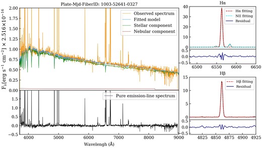
Example of FADO continuum (stellar and nebular) fits to an SDSS dwarf galaxy spectrum with the fits colour coded per the legend (top left) and the derived pure emission line spectrum (bottom left). The right upper and right lower panels, respectively, show the fitted Hα and Hβ lines, with the residuals shown at the bottom of each panel. The SDSS spectrum is from Plate = 1003, MJD = 52 641 FiberID = 0327.
Finally, the chosen wavelength range (see Cardoso et al. 2022) includes the noisier parts of the SDSS spectra. To see if the inclusion of these noisier parts of the spectra affected the robustness of the implicit stellar populations and, consequently, the determination of the galaxies’ nebular properties, we ran FADO limiting the spectral range to 4300–7000 Å. Using this less noisy spectral range, we found that the mean stellar ages weighted by light and mass are 0.944 and 2.393 Gyr, respectively. While using the full wavelength range, the mean stellar ages weighted by light and mass are 0.718 and 1.802 Gyr, respectively. We also found that the mean nebular properties differed by 2, 0, and 4 per cent for the Hα fluxes, log [N ii]/Hα, and log [O iii]/Hβ, respectively. This implies a difference of 0.01 dex for the mean 12 + log(O/H). In Section 3.1, we describe the methods used in this work to estimate the oxygen abundance. We conclude that our chosen SDSS spectral range does not materially affect the results or interpretations of this study.
2.3 Emission line flux
Emission line fluxes were derived from analysis of the candidates’ SDSS spectra. The SDSS spectra were derived from fibres with a 3 arcsec diameter within the wavelength range 3800–9200 Å. The fraction of a galaxy’s optical emission detected within this wavelength range depends on the dwarf’s angular diameter and redshift. The catalogued dwarfs have a mean SDSS fibre coverage fraction of the dwarfs’ deprojected optical discs of approximately ∼0.07. This fraction is based on a surface area estimated from the g-band Dpet × 1.5 which is approximately equal to D25 (see Section 1). Our calculation assumes that the galaxies are face-on and thus provides a lower limit for the fractional fibre coverage. Fig. 3 shows the distribution of the fibre coverage fraction for the catalogued dwarfs’ surface area based on their D25, extrapolated from their g-band Dpet. As a cross-check, the fibre coverage fraction was re-calculated using galaxy diameters from NED, which also gave a mean coverage fraction of ∼0.07. Using either method, we see that the spectra are typically based on the emission from less than 10 per cent of each dwarf’s surface area. However, the relatively small physical diameter of dwarfs and the short time-scale for metallicity homogenization across dwarfs (Croxall et al. 2009; Lagos et al. 2009, 2012; Lagos & Papaderos 2013, and references therein) mean we have no reason to consider that the metallicities derived from the SDSS spectra are unrepresentative of each dwarf’s whole surface area as would be the case for larger spiral galaxies with distinct bulge and disc components.
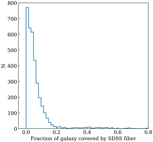
Histogram showing the distribution of the fraction of the catalogued dwarfs’ surface area covered by the SDSS spectral fibre (Dfiber = 3 arcsec). Each galaxy’s surface area was estimated from its SDSS g-band D25.
We applied the FADO code to the SDSS spectra of all potential members of our catalogue, as detailed in Section 2.1, to get pure and precise observed emission line fluxes. We then corrected for intrinsic extinction to derive intrinsic emission-line fluxes from integrated observed flux F(λ) using equation (2):
where f(λ) is the reddening function taken from Cardelli, Clayton & Mathis (1989) assuming R|$\mathrm{ v}$| = 3.1. The logarithmic reddening parameter c(Hβ) was calculated assuming case B (Osterbrock & Ferland 2006) for the Balmer decrement ratio, Hα/Hβ = 2.86 at 10 000 K.
As our catalogue is a subset of all galaxies with SDSS DR-16 spectra, it is useful to compare selected properties of our catalogued galaxies with the SDSS value-added catalogue produced by MPA–JHU.1 In Appendix A, Fig. A1 (left), we show the comparison of Hα and Hβ fluxes for our dwarf galaxies. The x-axes show values derived from our methods and the same properties from MPA–JHU on the y-axis. The emission line fluxes shown in Fig. A1 differ at 1σ level from the MPA–JHU catalogue values. Similar results to ours were obtained by Miranda et al. (2023). This difference is a known issue, which arises from different flux measurement methods.
2.4 BPT diagnostic diagram
Dwarf galaxies in our final catalogue consist of unclassified dwarfs and their spectra could potentially be dominated by an energy source other than stars, e.g. active galactic nuclei (AGN) or shocks. In Fig. 4, we use Baldwin, Phillips, Terlevich (BPT) diagnostic diagrams (Baldwin, Phillips & Terlevich 1981): log([N ii] λ6584/Hα) versus log([O iii] λ5007/Hβ), upper panel, and log([S ii] λλ6717,6731/Hα) versus log([O iii] λ5007/Hβ), lower panel, to determine the catalogued dwarfs’ ionization sources. The demarcation dashed curves in the figures are from the model by Kewley et al. (2001) (red line) and (Kaufmann et al. 2003) (black line). The lower left areas of both panels are H ii regions dominated solely by photoionization from hot young stars. The area at the top and right of the dashed red curves is inhabited by galaxies who’s dominant ionization mechanism is AGN and/or low-ionization nuclear emission-line region (LINER) emission. On the other hand the area between the two curves is the composite region, where both AGN/LINERs and SF contribute significantly to the ionization. In the upper panel of Fig. 4, we see that most galaxies fall in the locus predicted by models of photoionization by young stars. However, there are a few exceptions i.e. the 23 galaxies in the composite region of the N ii diagram and the one galaxy falling in the pure AGN region. Although, we did not detect asymmetric line profiles at the base of Hα lines for these 23 dwarfs, future observations may reveal the presence of AGN in this small subsample of our catalogue. Similarly, in the S ii BPT diagram, Fig. 4 lower panel, 181 galaxies fall in the AGN-dominated region. The fraction of AGN-dominated galaxies in both panels of the plot is very small.
![BPT log([N ii] λ6584/Hα) versus log([O iii] λ5007/Hβ) (upper panel) and log([S ii] λλ6717,6731/Hα) versus log([O iii] λ5007/Hβ) (lower panel) diagnostic diagrams for the 3459 galaxies in the dwarf catalogue. We include, in the diagrams, the Kewley et al. (2001; red dashed line) and Kaufmann et al. (2003; black dashed line) model boundary lines which divide regions dominated by photoionization, composite, and AGN/LINERs.](https://oup.silverchair-cdn.com/oup/backfile/Content_public/Journal/mnras/528/4/10.1093_mnras_stae390/1/m_stae390fig4.jpeg?Expires=1750259155&Signature=i~Js0j-HIxJWH8e7pGmhc1MEPInHD4edk9b5YqxA7IGDYnCW0NcSotmHJzNpMauL6UuHGBx3UyDId5A~mivaLr27KMTFZM7YRWkCaCu3PsDqXqngn8xWLhpNgl59Hbuj9Pvx6CU~d224Hb7PTJxYmBLHdhVg~FpsjYVnzAy-AdfOpERvRS09RRiC~KkPNU64X0ZgWYvT7AJjxwQ2RsbHorwnpBX557mRaaPmdPsqO7hXqidRpMiHr~E68Ibr3083Ax~6vQ8lTxvqchHskzY0p5qjQBm65GETVjd-Gu37Xm7EgECPS0kyOBNieHO2NNC7plBeq8KVjCosQFaCWcC9~w__&Key-Pair-Id=APKAIE5G5CRDK6RD3PGA)
BPT log([N ii] λ6584/Hα) versus log([O iii] λ5007/Hβ) (upper panel) and log([S ii] λλ6717,6731/Hα) versus log([O iii] λ5007/Hβ) (lower panel) diagnostic diagrams for the 3459 galaxies in the dwarf catalogue. We include, in the diagrams, the Kewley et al. (2001; red dashed line) and Kaufmann et al. (2003; black dashed line) model boundary lines which divide regions dominated by photoionization, composite, and AGN/LINERs.
3 RESULTS
3.1 Metallicity estimates
The BPT diagrams, in Section 2.4, show that the majority of the galaxies in our catalogue are local star-forming dwarf galaxies. This demonstrates that our sample is consistent with the samples used for calculating metallicity of local H ii galaxies (Terlevich et al. 1991) in Denicoló, Terlevich & Terlevich (2002), Pettini & Pagel (2004), and Pérez-Montero & Contini (2009), where the 12 + log(O/H) abundance is characterized using H ii-based calibrators. The direct Te method for determining a galaxy’s metallicity is generally considered the most accurate and uses [O iii] λ4363 and λλ4959, 5007 lines and the [O ii] λ3727 doublet to estimate oxygen abundance. However, the weak [O iii] λ4363 auroral emission line is difficult to detect. Moreover, in the redshift range of our candidates, the [O ii] λ3727 spectral line appears within a noisy region very close to the edge of the SDSS spectrometer wavelength range or is redshifted beyond the spectrometer’s wavelength range. As a result, we detect the lines needed to apply Te method in only about half of the galaxies in our catalogue. Because of these constraints, the errors in applying the Te method can be large. Therefore, we use the alternative strong line calibrators to estimate the metallicities of the dwarf galaxies more consistently and accurately. We compute oxygen abundances using several of these diagnostic methods (see the list of calibrators used in Table 1) and the following indexes:
and
Mean metallicity for the dwarf galaxy catalogue from the N2- and O3N2-based calibrators used in this study.
| Calibrator | Reference | Mean | Standard deviation |
|---|---|---|---|
| N2 | Bian2018 | 8.39 | 0.14 |
| N2 | Curti2020 | 8.45 | 0.12 |
| N2 | Denicoló2002 | 8.44 | 0.16 |
| N2 | Marino2013 | 8.31 | 0.10 |
| N2 | Nagao2006 | 8.45 | 0.20 |
| N2 | Pérez–Montero2009 | 8.33 | 0.18 |
| N2 | Pettini2004 | 8.33 | 0.12 |
| O3N2 | Bian2018 | 8.49 | 0.20 |
| O3N2 | Curti2020 | 8.51 | 0.20 |
| O3N2 | Marino2013 | 8.28 | 0.09 |
| O3N2 | Pérez–Montero2009 | 8.37 | 0.13 |
| O3N2 | Pettini2004 | 8.35 | 0.12 |
We summarize below the calibrators used in this study:
The calibrations from Pettini & Pagel (2004), Denicoló, Terlevich & Terlevich (2002), and Pérez-Montero & Contini (2009) come from nearby H ii galaxies, using the Te method, and their subsamples of dwarf irregular galaxies using mainly N2 and O3N2 indexes. Some additional diagnostics are as follows:
Marino et al. (2013) also used Te-based measurements but for H ii regions from the CALIFA sample and 603 H ii regions from the literature.
Bian, Kewley & Dopita (2018) used the spectra of a sample of local MPA–JHU SDSS analogues of high-redshift galaxies.
Nagao, Maiolino & Marconi (2006) also used data from the SDSS but with known metallicity available from the literature and gave an analytical description for the metallicity dependence of the many diagnostics and line ratios within the metallicity range 7.0 ≤ 12 + log(O/H) ≤ 9.2.
Curti et al. (2020) determined the metallicity via the Te method in SDSS star-forming galaxies with z > 0.027, the diagnostics proposed in that work were calibrated against metallicity in the range 7.6 ≤ 12 + log(O/H) ≤ 8.9.
Fig. 5 shows the metallicity distribution for our dwarf galaxy catalogue for all diagnostics used in our study, i.e. N2 (left panel), O3N2 (middle panel), and the average of all calibrators used in this study (right panel). In Table 1, we show the mean metallicity and standard deviation for our catalogued dwarf galaxies for each of the methods described above. It is well known that N2 depends on the ionization parameter. O3N2 also depends on the ionization parameter, but to a lesser extent than N2. According to Zurita et al. (2021), O3N2 overestimates gas-phase metallicities for low-metallicity galaxies. However, the dwarf catalogue galaxies have near solar metallicities. We compared the mean 12 + log(O/H) for the dwarfs in our catalogue derived from O3N2+N2 and O3N2 and N2 calibrators and found no difference between them within the uncertainties, see Table 2.
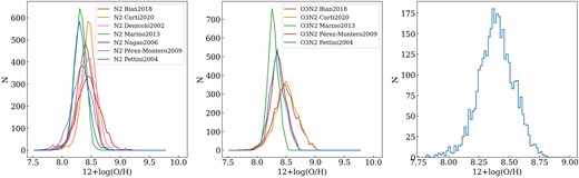
Metallicity distribution for our dwarf galaxy catalogue using N2 (left panel) and O3N2 (middle panel) calibrators and the average of all these calibrators, listed in Table 1, (right panel).
Dwarf galaxy catalogue properties.
| Property | Mean | Standard deviation | Unit |
|---|---|---|---|
| 12 + log(O/H) O3N2+N2 | 8.39 | 0.15 | |
| 12 + log(O/H) N2 | 8.38 | 0.15 | |
| 12 + log(O/H) O3N2 | 8.39 | 0.13 | |
| EW(Hβ) | 18.80 | 24.27 | Å |
| g-band magnitude | −16.53 | 1.35 | mag |
| g-band D25 | 5.48 | 1.99 | kpc |
| Redshift | 0.017327 | 0.00816 | |
| g − i colour | 0.52 | 0.47 | mag |
| log(M*) | 8.43 | 0.74 | M⊙ |
| log(SFR) | −1.32 | 0.67 | M⊙ yr−1 |
As our catalogue contains dwarfs with a range of properties, no particular calibrator is ideal for all cases; so, for our analysis, we utilize the 12 + log(O/H) for each catalogued dwarf’s abundance using the average of the metallicity from all of O3N2 and N2 calibrator methods listed in Table 1. Appendix A contains a comparison of our metallicity results with those produced by MPA–JHU. From that comparison, we can say that our metallicity estimates show a similar trend to MPA–JHU if we use the same strong line calibrations.
Additionally, we calculated the electron density ne from the emission line ratio [S ii]λ6717/[S ii]λ6731, assuming Te(O iii) = 10 000 K, using temden implemented within the iraf2nebular software package. Fig. 6 shows the resulting distribution of electron densities for the catalogued dwarfs with non-saturated electron densities. We found that only 1780 galaxies, in our catalogue, have non-saturated electron density values ([S ii]λ6717/[S ii]λ6731 < 1.43). In that subsample, most galaxies show low electron density values of the order of ∼100 cm−3 which is normal for star-forming dwarf galaxies (e.g. Masegosa, Moles & Campos-Aguilar 1994; Bordalo & Telles 2011).
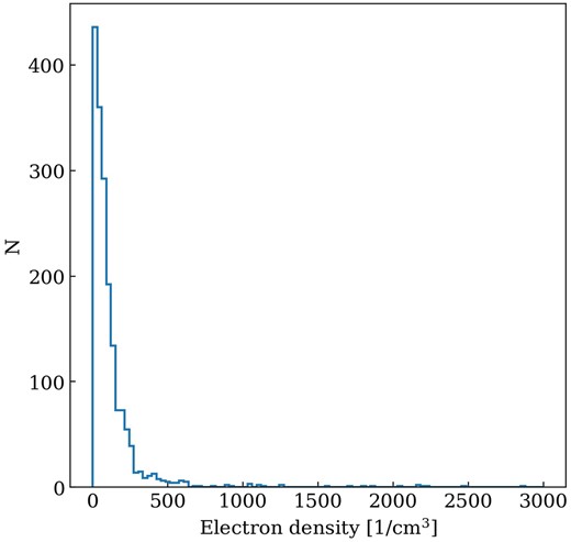
The distribution of electron densities for the dwarfs in our catalogue with non-saturated electron densities.
3.2 SFR determination
For each galaxy in the catalogue, we estimate the SFR from it’s Hα luminosity L(Hα) using the Kennicutt (1998) conversion, which assumes a Salpeter IMF and solar metallicity. To ensure consistency amongst our measurements we then made a conversion to a Chabrier (Chabrier 2003) IMF, i.e. SFR(Hα) (M⊙ yr−1) = L(Hα)/1041.31 erg s−1 (Miranda et al. 2023). We compared our SFR estimates with the MPA–JHU catalogue in Appendix A. The fluxes in the MPA–JHU catalogue are normalized to match the photometric r-band fibre magnitude. This normalization factor was derived from the MPA–JHU catalogue and was applied to the galaxies in our catalogue. We also converted the MPA–JHU SFR(Hα) (Kroupa IMF) to Chabrier IMF by decreasing the MPA–JHU SFR (Kroupa IMF) by 0.03 dex (Miranda et al. 2023) to enable comparison with our SFR(Hα) (see Appendix A). The 3 arcsec diameter SDSS fibres cover only a small fraction of our dwarfs’ disc areas, see Section 2.3. So, the SFR(Hα) estimated from the SDSS fibre data alone would in almost most cases underestimate the SFR(Hα) of our catalogued dwarfs. Thus as a final step, to estimate the total SFR(Hα) of the catalogue dwarfs, we used the aperture correction procedure prescribed in section 4.1 of Miranda et al. (2023). We use the aperture-corrected SFR(Hα) values of our dwarfs for our analysis throughout the paper and these values are presented in the online catalogue and Table 3. The only exception is the comparison with MPA–JHU in Appendix A which is a comparison of SFR(Hα)s before aperture correction.
Dwarf galaxy catalogue – example.
| SpecObjID | RA | Dec | SDSSname | Redshift | g − i | D25 | log(M*) | log(SFR) | EW(Hβ) | 12+log(O/H) | Flag |
|---|---|---|---|---|---|---|---|---|---|---|---|
| [hms] | [dms] | [kpc] | [M⊙] | [M⊙ yr−1] | [Å] | ||||||
| 1a | 2 | 3 | 4 | 5 | 6 | 7 | 8 | 9 | 10 | 11 | 12 |
| Galaxy1 | 9h48m42.33s | −0d21m14.50s | SDSS J094842.33−002114.5 | 0.00628 | 0.76 | 4.2 | 8.20 | −1.87 | 4.89 | 8.37 ± 0.08 | 1 |
| Galaxy2 | 9h41m17.02s | +0d46m16.00s | SDSS J094117.02+004615.9 | 0.00658 | 0.69 | 1.9 | 7.88 | −1.90 | 6.98 | 8.42 ± 0.09 | 1 |
| Galaxy3 | 9h44m10.90s | +0d10m47.17s | SDSS J094410.90+001047.1 | 0.01112 | 0.73 | 5.0 | 8.67 | −1.09 | 65.71 | 8.28 ± 0.05 | 1 |
| Galaxy4 | 9h47m05.50s | +0d57m51.24s | SDSS J094705.50+005751.3 | 0.00618 | 1.00 | 6.3 | 8.58 | −2.59 | 19.63 | 8.28 ± 0.06 | 0 |
SpecObjID is the SDSS identification number unique to each pointing. Due to lack of space, the SpecObjID has been shortened and represented as Galaxy1, Galaxy2, etc., in the first column. The complete IDs are the following: 299496824270514176, 299582311299573760, 299619694694918144, 299647182485612544, respectively. The online version of Table 3 contains the complete SpecObjectIDs in column 1.
3.3 Dwarf galaxy catalogue
Our final dwarf catalogue contains 3459 galaxies and is available online (see Appendix B). Table 3 shows a truncated version of the catalogue with example entries. The columns in the table are as follows:
(1) The SDSS SpecObject ID.
(2 and 3) RA DEC J2000 positions.
(4) SDSS galaxy name.
(5) SDSS spectroscopic redshift.
(6) g − i SDSS model magnitude colour.
(7) D25 [kpc].
(8) log(M*) [M⊙].
(9) log(SFR(Hα)) [M⊙ yr−1].
(10) EW(Hβ) [Å].
(11) 12 + log(O/H) and 1σ uncertainty. Mean of values for each dwarf is derived from all N2 and O3N2 calibrators listed in Table 1.
(12) SDSS photometery flag, 0 = not clean, 1 = clean, 2 = derived M* or g − i colour is unrealistic.
The majority of our catalogued dwarfs have stellar masses between ∼108 and 109 M⊙ (see Fig. 1), which are normal values for dwarf galaxies. Although the catalogue does contain a small fraction of low stellar mass dwarfs with stellar masses <107 M⊙. Fig. 5 (right panel) shows the distribution of the mean 12 + log(O/H) for the galaxies in the catalogue. The catalogue’s mean 12 + log(O/H) value is ∼8.39 ± 0.15. This mean value falls towards the upper end of the range of expected 12 + log(O/H) of 7.4 to ≲ 8.4 referred to in Section 1. The absence of the lowest metallicity XMP dwarfs is likely the result of applying the 2.5σ line emission SNR selection criterion to the catalogue. No correlation between the catalogue’s 12 + log(O/H) and redshift was found. For further detail about metallicity and its calibration, see Section 3.1.
The distributions of Dpet [kpc], SDSS g − i colour, log(M*/M⊙), and redshift for the galaxies in the catalogue are shown in Fig. 1. The top left panel of Fig. 1 shows that the catalogue’s dwarfs have mean Dpet = 3.66 ± 1.33 kpc (D25 = 5.48 ± 1.99 kpc). This confirms that their D25 diameters lie within the ∼0.1–10 kpc range expected for dwarf galaxies, in Section 1. Table 2 gives the catalogue’s mean values and the standard deviations for 12 + log(O/H), EW(Hβ), SDSS g-band magnitude, D25g-band diameter, redshift, g − i colour, log(M*), and log(SFR(Hα)) (total SFR) calculated as described in Section 3.2.
As expected, the stellar mass distribution in the catalogue (Fig. 1) strongly favours dwarfs with masses near our catalogue’s M* upper limit (1 |$\times $| 109M⊙), because such dwarfs being more luminous have a much higher probability of having an SDSS spectral observation than less luminous dwarfs. Moreover, more massive star-forming dwarfs have a higher probability of fulfilling our emission line SNR criteria. The catalogue’s dwarfs have a mean M* = 2.7 |$\, \times$| 108 M⊙, i.e. similar to the Small Magellanic Cloud, M* = 3.1 × 10⁸ M⊙ (van der Marel, Kallivayalil & Besla 2009).
A g − i colour of 1.1 approximately coincides with the red-sequence threshold displayed in the colour–magnitude plot in fig. 12 of Cortese et al. (2008). The galaxies in our catalogue have a mean SDSS g − i colour of 0.52 ± 0.47 (top right panel of Fig. 1). On average, the galaxies in the catalogue have a g − i colour < 1.1, unambiguously qualifying them as blue galaxies. This confirms that the catalogue is dominated by dwarfs which have experienced a recent episode of SF. We note that our catalogued dwarfs do not display the bimodal colour distribution seen in some other samples, e.g. the LSB galaxies in Bhattacharyya et al. (2023). The absence of dwarfs with red colour in the catalogue is likely to be the result of our selection bias, see Section 4.1. We see from the bottom right panel of Fig. 1 that the catalogue’s redshift distribution has several maxima with two of the most prominent at z ∼ 0.006 and z ∼ 0.023. The number of dwarfs between z ∼ 0.025 and 0.03 declines rapidly, reflecting the rapid fall off of completeness of SDSS dwarf galaxies meeting our criteria beyond z ∼ 0.025. The redshift and spatial distribution of catalogue’s dwarfs are discussed further in Section 4.2.
4 DISCUSSION
4.1 Mass–metallicity/SFR relations
This subsection investigates the stellar mass gas–metallicity relation of our catalogue, within a stellar mass range of log(M*/M⊙) ∼ 6 to 9, in comparison to other samples. This relation has been reported for massive galaxies by several authors (e.g. Tremonti et al. 2004; Gallazzi et al. 2005) and for dwarf galaxies in a similar mass range to our catalogue (e.g. Jimmy et al. 2015). As M* values in the relation depend on robust photometry, for this analysis we used a subsample of our catalogue (n = 2568) restricted to galaxies with a clean photometry flag = 1, in Table 3.
In Fig. 7, we compare the values from our subsample with those from Lee et al. (2006), Berg et al. (2012), James et al. (2015), Jimmy et al. (2015), and Li et al. (2023). In the same figure, we show a spline fit (K = 5) to our data for dwarfs in the stellar mass range log(M*/M⊙) = 7.5–9. We see from the fit to our data that our 12 + log(O/H) values, based on the mean of O3N2 and N2 calibrators, are in good agreement, within the uncertainties, with those from Jimmy et al. (2015) in the mass range log(M*/M⊙) ∼ 8–9. However, our 12 + log(O/H) values are systematically higher for the same stellar mass compared to those from Lee et al. (2006), Berg et al. (2012), and James et al. (2015).
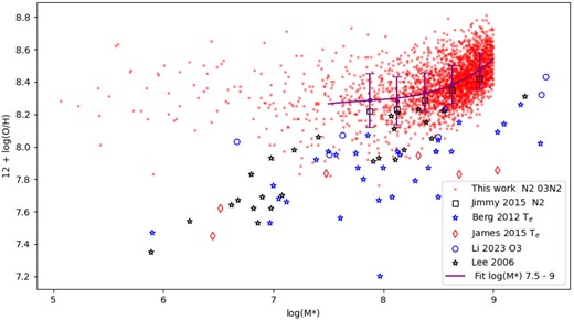
Mass–metallicity relation, 12 + log(O/H) versus log(M*/M⊙), for the subsample of dwarfs in our catalogue with clean SDSS photometry compared to values from the literature (see the text). A spline (k = 5) fits to 12 + log(O/H) versus log(M*/M⊙) for our subsample for dwarfs, in the log(M*/M⊙) range 7.5–9, is shown with a magenta line. Additionally, magenta dots show the mean with 1σ uncertainty error bars for our subsample’s 12 + log(O/H) values, in the same mass bins used by Jimmy et al. (2015).
The plot also shows values from higher redshift (z = 2–3) dwarfs from Li et al. (2023). The slope of their relation becomes shallower at log(M*/M⊙) ⪅ 8.5, similar to trends seen in our data and Jimmy et al. (2015). In contrast, the Berg et al., James et al., and Lee et al. data imply that the gradient of the relation found at log(M*/M⊙) ⪆ 8.5 remains constant down to stellar masses as low as log(M*/M⊙) ∼ 6.
The Berg et al. and James et al. 12 + log(O/H) values are derived from long-slit Multiple Mirror Telescope (MMT) spectra which could potentially be more representative of the metallicity of the whole galaxy compared to the more limited sampling at the centre of dwarfs by the SDSS fibre aperture for our catalogue. However, the expected rapid dispersion of metals in dwarfs (e.g. Kobulnicky & Skillman 1996; Croxall et al. 2009; Lagos et al. 2009, 2016) argues against this as an explanation for the large observed differences between the samples. Because of the limited SDSS spectral coverage, Jimmy et al. (2015) use N2 and we use N2 and O3N2 calibrators rather than the preferred direct method (Te) to determine 12 + log(O/H). However, the 12 + log(O/H) N2 and O3N2 calibrators used in this study are formulated to give similar results to the Te method. It is therefore highly unlikely that the adopted calibrator(s) alone are responsible for the differences in mass–metallicity slopes in different samples observed in Fig. 7.
To analyse and ascertain the exact reasons for the differences in the results in Fig. 7 is beyond the scope of this paper. The [O iii]λ4363 line is faint in subsolar metallicity where metal cooling is more efficient. This leads us to use strong-line calibrators instead of the Te-based method to calculate the oxygen abundance. However, we consider our emission-line SNR criterion to be the principal reason why the mean metallicity in each mass bin shows a systematically higher metallicity compared to the other samples in Fig. 7. Our SNR criterion led to the exclusion of metal-poor dwarfs with weak emission lines from our calculation of the mean metallicity of each mass bin. This had the effect of raising the calculated mean metallicity of each mass bin compared to the underlying metallicity of the bin’s dwarfs.
Additionally, there is a trend for emission lines to become proportionately weaker with decreasing stellar mass. Therefore, as stellar mass decreases the fraction of dwarfs able to meet our SNR criterion also decrease. This declining fraction meant that the reported mean metallicities of successively lower mass bins were based on increasingly unrepresentative samples of high-metallicity dwarfs and an under-representation of the bin’s underlying and predominantly low-metallicity dwarf population. We, therefore, consider this progressive under-representation of the low-mass low-metallicity population is likely to be responsible for the apparent flattening of mean metallicity derived for the mass bins, below log(M*/M⊙) ∼ 8.5 in Fig. 7.
Using chemical evolution models, Recchi, Kroupa & Ploeckinger (2015) investigated the chemical evolution of ancient TDGs formed out of metal-poor baryonic tidal interaction debris at high redshifts. They found that such ancient TDGs formed out of gas with initially very low metallicity naturally increase their metallicity to follow the linear mass–metallicity relation for local dwarf galaxies from Lee et al. (2006), see Fig. 7 and fig. 1 in Recchi, Kroupa & Ploeckinger (2015). In contrast, TDGs formed at lower redshifts from metal-enriched baryonic debris are observed to be outliers above the mass–metallicity relation at log(M*/M⊙) ⪅ 9, see fig. 1 in Recchi, Kroupa & Ploeckinger (2015). Interestingly, the shallower mass–metallicity relation for our catalogue is similar to the one reported by Recchi, Kroupa & Ploeckinger (2015) for more recently formed high-metallicity TDGs (Boquien et al. 2010; Duc et al. 2014). We speculate this similarity may indicate that our catalogue could contain a significant number of TDGs formed at lower redshifts. However, this seems highly unlikely to be the explanation for the bulk of catalogue members.
Fig. 8 shows the log(SFR/M⊙ yr−1) versus log(M*/M⊙) for the catalogue. Since this relation requires M*, the figure uses same subsample we used for mass–metallicity analysis. The figure also shows a linear fit to our subsample data. Additionally, the plot shows the linear fits to the relations from Duarte Puertas et al. (2017) and Miranda et al. (2023) for the SDSS galaxies in their samples. The slope of the fit to our data (black line) is in good agreement with the one from Duarte Puertas et al. (2017) (red line) which is derived from SDSS spectra with aperture corrections based on the CALIFA IFU survey observations. This agreement confirms that our aperture corrections for the clean photometry subsample are reasonable. However, the slope of the fit to our subsample is slightly steeper and offset compared to the fit to Miranda’s SDSS sample (green line), which is dominated by main-sequence star-forming galaxies with log(M*/M⊙) > 9.
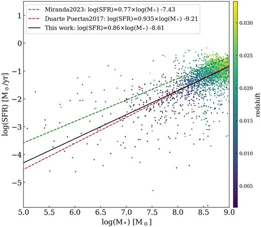
A plot of log(SFR/M⊙ yr−1) against log(M*/M⊙) for the subsample of dwarfs in our catalogue with clean SDSS photometry. The linear fit to our subsample data is shown with black line. To compare to our fit to the literature, we also show linear fits from Duarte Puertas et al. (2017) – red dashed line, and Miranda et al. (2023) – green dashed line. See the text for comments on the slope differences.
4.2 Environment
The redshift distribution of the catalogue’s dwarfs, Fig. 1 bottom right panel, shows multiple maxima, with the vertical lines on the plot indicating the redshifts of the Virgo and Coma clusters. Two of the catalogue’s redshift maxima are near, but not coincident with, the redshifts of Virgo and Coma. Fig. 9 plots the sky positions of the dwarf (top row) and non-dwarf galaxies (bottom row) with SDSS spectra, each divided into four redshift bins. The colour of the points corresponds to the relative redshift of the galaxies within each redshift bin, with blue points representing lower redshift galaxies and red points, those with higher redshifts. The sizes of the Virgo and Coma clusters based on their respective virial radii (rvir) of 6○ or 1.7 Mpc (Mei et al. 2007) and ∼1.5○ or ∼3 Mpc (Łokas & Mamon 2003) are shown in the figure with ellipses. It is clear from Fig. 9 that the dwarfs in our catalogue are not preferentially associated with the Virgo and Coma galaxy clusters as might be suggested by the redshift distribution in Fig. 1 – bottom right panel. Instead, they are distributed across much larger redshift and spatial scales. For dwarfs with velocities below 7500 |${\rm km}\, {\rm s}^{-1}$|, their distribution in RA, DEC, and redshift space traces the same filamentary structures traced by the SDSS non-dwarf galaxy population with spectra. At velocities above 7500 |${\rm km}\, {\rm s}^{-1}$| (z = 0.025), the association between the dwarf and non-dwarf galaxies remains only for the lowest redshift dwarfs. For dwarfs with higher redshifts in this bin, the association between the populations progressively dissolves with increased redshift, with few dwarfs meeting our selection criteria at the highest redshifts. We conclude that at velocities below ∼ 5000 |${\rm km}\, {\rm s}^{-1}$| the catalogued dwarfs trace lower-density large-scale galaxy structures reasonably well, but above 5000 |${\rm km}\, {\rm s}^{-1}$| the association between dwarf and non-dwarf galaxies increasingly weakens, due to the relative incompleteness of the dwarfs in our catalogue.
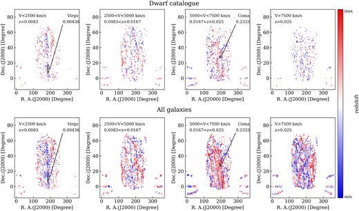
Sky distribution of the SDSS-DR16 galaxies with spectra in four redshift bins (columns): The top row shows the catalogued dwarf galaxies and the bottom row all non-dwarf galaxies with SDSS spectra. The relative redshifts of galaxies within each redshift bin are indicated with the colour per the colour scale. The Virgo and Coma galaxy clusters’ sky positions and sizes are shown in the figure with the larger and smaller ellipses, respectively.
To assess the effect of the local environment on the catalogue’s properties, we carried out an analysis of the impact of tidal forces within a limited volume surrounding each catalogued dwarf and the tidal forces acting on the dwarf arising from its nearest neighbour, as follows:
Byrd & Valtonen (1990) investigated the triggering of nuclear SF from tidal encounters in Seyfert galaxies using a tidal perturbation parameter, Pgg, (equation 5):
where Mc = M* of the nearest companion galaxy, Mg = M* of the target galaxy, r is the projected distance between the two galaxies, and A is the optical disc radius of the target. While the threshold for triggering SF depends on the specifics of the interaction, our analysis assumes that the tidally induced SF threshold is in the Pgg range of 0.006–0.1 from Byrd & Valtonen (1990).
To define the environment of isolated galaxies (Verley et al. 2007) developed a tidal force parameter, which is a measure of the sum of tidal forces acting on a galaxy in comparison to the binding force within it. In our analysis, we modified Verley’s tidal force parameter to include only companions with SDSS spectroscopic redshifts within a radius of 500 kpc and velocities within ± 300 |${\rm km}\, {\rm s}^{-1}$| of the target galaxy. Our tidal force parameter (Q0.5–300) takes into account both the projected separation distance and the M* of the companions, calculated as follows:
where Mi = the companion’s M*, Mg = the target’s M*, Dg is the target’s D25, and Sig is the projected distance between the companion and the target galaxy. Values used for these calculations were extracted from the SDSS online data base, with D25 = 1.5DPetrosian and M*, calculated using the SDSS g and i model magnitudes together with coefficients from Bell et al. (2003). The Q0.5–300 parameter focuses on companions which could potentially have interacted with the target galaxy within the last ∼1 Gyr, so could have conceivably triggered SF in the target galaxy. Because our analysis is limited to galaxies with SDSS redshifts, we are excluding companions which lack SDSS redshifts, and the impact of this limitation increases with redshift.
Fig. 10 plots the tidal perturbation parameter Pgg against the Q0.5–300 parameter for our sample dwarfs with the g − i colour of the galaxies per the colour scale. The figure plots the same clean photometry subsample (n = 2568) used in Section 4.1. We used this subsample because Pgg and Q0.5–300 require parameters derived from SDSS photometry. Limiting our analysis to the clean photometry subsample improves the reliability of our analysis. The region between horizontal lines on the figure indicates the Pgg threshold range for tidally induced SF from Byrd & Valtonen (1990). 1112 of the subsample galaxies (43 per cent) did not have a Q0.5–300 companion. Only 96 subsample dwarfs (3.7 per cent) lie within or above the Pgg threshold range for tidally induced SF. These 96 dwarfs are bluer than the vast bulk of the subsample which indicates that the vast majority of the subsample is currently relatively isolated, with only a small fraction having a Pgg parameter and colour consistent with having undergone a recent tidal interaction.
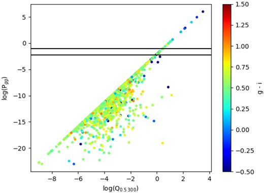
Nearest neighbour induced star formation parameter, log(Pgg) versus log(Q0.5–300) sum of near neighbour tidal forces parameter, for our subsample of dwarf galaxies with clean photometry flags in SDSS. The horizontal lines show the threshold range for tidally induced star formation (Byrd & Valtonen 1990). The g − i colour of the galaxies is per the colour scale.
log(Pgg) and log(Q0.5–300) values are based on the galaxies’ current projected separation. It follows from the definition of Q0.5–300 that all 1456 dwarfs in the plot could potentially have been close enough to their nearest companion to have crossed the tidally induced log(Pgg) SF threshold within the past ∼1 Gyr. However, the 1456 dwarfs present a narrow range of blue colour 0.56 ± 0.25. Moreover, leaving aside the 96 with the closest companions, the subsample lacks a g − i colour trend with either log(Pgg) or log(Q0.5–300), suggesting that recent interactions are not driving the SF in subsample. Plots with the same log(Pgg) and log(Q0.5–300) axes as Fig. 10 but using 12 + log(O/H) and log(SFR) for the colour axes showed no trend between environment and 12 + log(O/H) or log(SFR).
4.3 EW(Hβ) distribution and SFR
The EW(Hβ) distribution of our catalogue is shown in Fig. 11 (left panel). This panel compares our results (mean log(EW(Hβ)/Å) = 1.11) with those for strongly star-forming dwarfs (H ii/BCD galaxies) in the literature by Lagos, Telles & Melnick (2007) and Bordalo & Telles (2011) (mean log(EW(Hβ)/Å) =1.56 and 1.78), respectively. EW(Hβ) has been used as an indicator of the age of the current burst of SF (e.g. Copetti, Pastoriza & Dottori 1986), with younger starbursts having higher EW(Hβ) values. The EW(Hβ) distribution for our catalogue spans a lower range of values compared to strongly star-forming H ii/BCD galaxies, which indicates higher mean stellar ages for the current burst.
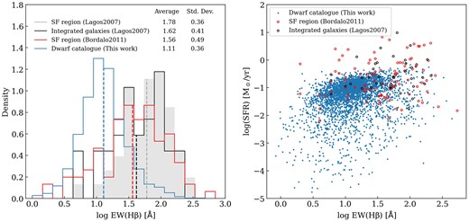
EW(Hβ) distribution for our catalogue of galaxies in comparison to distributions from the literature per the legend (left panel). SFR versus EW(Hβ) for our catalogue compared to literature samples per the legend (right panel).
In the right-hand panel of Fig. 11, we see the average log(SFR/M⊙ yr−1) for the H ii/BCD galaxies is higher than that for our catalogue.We find a mean log(SFR/M⊙ yr−1) of −1.32, while the mean log(SFR/M⊙ yr−1) of the H ii/BCD galaxies are −-0.59 for the Bordalo & Telles (2011) sample and −0.57 for the Lagos, Telles & Melnick (2007) sample. Interestingly, the mean log(SFR/M⊙ yr−1) of our catalogue is between the mean log(SFR) of the H ii/BCD galaxies and the mean value of gas-rich LSB dwarfs (–2.04) (McGaugh, Schombert & Lelli 2017).
Gas infalls/interactions have been invoked to explain the SF activity in most H ii/BCD galaxies (e.g. Pustilnik et al. 2001; Lagos et al. 2018). But according to McGaugh, Schombert & Lelli (2017), the shallower SFR–log(M*) relation slope for dwarf LSBs, compared to strongly star-forming H ii/BCD galaxies, can be explained without invoking gas accretion/interactions to sustain their SF. This suggests that the moderate level of SF observed in most of our subsample dwarfs likely arises from stochastic SF bursts in relatively isolated dwarfs. This scenario is consistent with the finding in Section 4.2 that the overwhelming majority of the subsample dwarfs are relatively isolated and inhabit a rather narrow g − i colour range.
4.4 An overview (a possible scenario)
Recent work by Cattorini et al. (2023) showed that galaxies in filaments with the same redshift range as our catalogue display H i deficiencies and these deficiencies increase with proximity to the filaments (Crone Odekon et al. 2018). A reasonable explanation for these observations is interactions between galaxies in the filaments are removing H i from the filament galaxies. Section 4.2 shows that the distribution of our catalogued dwarfs traces local galaxy filaments and it would be reasonable to expect dwarf galaxies in such filaments to be disproportionately impacted by intra-filament interactions, including interactions which generate high-metallicity dwarfs, e.g. TDGs. From Section 4.1, we see that our catalogued dwarfs have near solar metallicities comparable to TDGs formed within the last few Gyrs (Duc 2012). It would be interesting to investigate with future observations whether intra-filament interactions are capable of driving dwarf metallicities to the levels observed in our subsample particularly at masses below log(M*/M⊙) = 8.5.
5 CONCLUDING REMARKS
We present a catalogue of 3459 blue, nearby dwarf galaxies (M* from 105 to 109 M⊙) extracted from SDSS DR-16 together with robust estimates of their metallicities. The strict spectral line SNR criterion used in our sample selection biased our sample towards star-forming dwarf galaxies with bright emission lines, but it achieved the goal of creating a catalogue of nearby SDSS dwarf galaxies with robust metallicity estimates.
The catalogue was compiled as follows: galaxies with radial velocity, 500 |${\rm km}\, {\rm s}^{-1}$| ≤ velocity ≤ 10 000 |${\rm km}\, {\rm s}^{-1}$|(0.00166 ≤ z ≤ 0.03333). To eliminate the massive galaxies, only sources with absolute magnitude Mg ≥ −18 mag, stellar mass ≤ 109 M⊙, and an optical diameter (D25) ≤ 10 kpc were retained. For a robust estimation of metallicities, we further limited our catalogue to galaxies where the emission lines used to determine the metallicities (Hβ 4861Å, [O iii] 5007Å, Hα 6563Å, [N ii] 6584Å, [S ii] 6717Å, [S ii] 6731Å) all had an SNR ≥ 2.5.
We compared the mass–metallicity relation from our clean photometry subsample of the catalogue with those derived from other dwarf samples. The most likely explanation for our systematically higher metallicities compared to all the other samples shown in Fig. 7 is our exclusion of low-metallicity galaxies as a result of our emission line SNR criterion. Applying this criterion results in the exclusion of an increasing fraction of galaxies as stellar masses decreased and is likely the cause of the apparent flattening of mean metallicity seen in our mass–metallicity relation, log(M*/M⊙) ∼ 8.5.
The shallower mass–metallicity relation for our catalogue is similar to the one reported for recently formed high-metallicity TDGs (Recchi, Kroupa & Ploeckinger 2015). This could suggest that at least a fraction of our catalogue dwarfs could have tidal origin. However, we refrain from making any strong claim about this as this is merely a speculation based on just the similarity of slopes from Boquien et al. (2010) and Duc et al. (2014). Future planned high-resolution studies of these dwarfs will reveal more about their formation scenarios.
Our analysis of the impact of near neighbours reveals that the majority of the clean photometry dwarfs are relatively isolated. However, the few clean photometry dwarfs, with tidally induced SF parameters above the Pgg threshold, display bluer g − i colours than these rest of the clean photometry dwarfs.
The mean EW(Hβ) of the catalogued dwarfs is nearly an order of magnitude lower than for samples of dwarfs with high SF rates, e.g. HII/BCD galaxies. Moreover, the mean SFR of the catalogued dwarfs is between the high star-forming BCDs and low star-forming LSBs. This together with the narrow colour range, and relative isolation of the vast majority of the catalogue’s clean photometry dwarfs, is consistent with a scenario in which the observed SF in the vast majority of the catalogued dwarfs arises from internally driven episodic mild bursts of SF rather than being driven by external interactions. Although, resolved multiwavelength observations would be required to confirm this.
This catalogue will be useful for the following categories of future investigations: (1) resolved studies of subsets of the catalogue focused on metallicity evolution, gas infall/accretion, and SF; (2) statistical studies of global properties of nearby dwarfs, especially high metallicity dwarf studies; (3) selection of subsamples for multiwavelength studies (e.g. optical and H i/CO/radio continuum).
ACKNOWLEDGEMENTS
We would like to thank the anonymous referee for his/her comments which have led to considerable improvements in the paper. YG acknowledges support from the National Key Research and Development Program of China (2022SKA0130100) and the National Natural Science Foundation of China (grant No. 12041306). PL (10.54499/DL57/2016/CP1364/CT0010) and TS (10.54499/DL57/2016/CP1364/CT0009) are supported by national funds through Fundação para a Ciência e a Tecnologia (FCT) via the Centro de Astrofísica da Universidade do Porto (CAUP). This research has made use of the Sloan Digital Sky Survey (SDSS), http://www.sdss.org/. Funding for the Sloan Digital Sky Survey IV has been provided by the Alfred P. Sloan Foundation, the U.S. Department of Energy Office of Science, and the Participating Institutions. SDSS-IV acknowledges support and resources from the Center for High-Performance Computing at the University of Utah. The SDSS website is www.sdss.org. SDSS-IV is managed by the Astrophysical Research Consortium for the Participating Institutions of the SDSS Collaboration including the Brazilian Participation Group, the Carnegie Institution for Science, Carnegie Mellon University, the Chilean Participation Group, the French Participation Group, Harvard-Smithsonian Center for Astrophysics, Instituto de Astrofísica de Canarias, The Johns Hopkins University, Kavli Institute for the Physics and Mathematics of the Universe (IPMU)/University of Tokyo, Korean Participation Group, Lawrence Berkeley National Laboratory, Leibniz Institut für Astrophysik Potsdam (AIP), Max-Planck-Institut für Astro- nomie (MPIA Heidelberg), Max-Planck-Institut für Astrophy- sik (MPA Garching), Max-Planck-Institut für Extraterrestrische Physik (MPE), National Astronomical Observatories of China, New Mexico State University, New York University, Uni- versity of Notre Dame, Observatário Nacional/MCTI, The Ohio State University, Pennsylvania State University, Shanghai Astronomical Observatory, United Kingdom Participation Group, Universidad Nacional Autónoma de México, Univer- sity of Arizona, University of Colorado Boulder, University of Oxford, University of Portsmouth, University of Utah, University of Virginia, University of Washington, University of Wisconsin, Vanderbilt University, and Yale University (Ahumada et al. 2020 ApJS 249, 3). This research has made use of the NASA/IPAC Extragalactic Database (NED) which is operated by the Jet Propulsion Laboratory, California Institute of Technology, under contract with the National Aeronautics and Space Administration.
DATA AVAILABILITY
We used archival SDSS DR-16 data in the catalogue presented in this paper. The full catalogue is published as an online table.
Footnotes
Image Reduction and Analysis Facility (IRAF) is distributed by the National Optical Astronomy Observatories, which are operated by the Association of Universities for Research in Astronomy, Inc., under cooperative agreement with the National Science Foundation.
References
APPENDIX A: A COMPARISON WITH THE MPA–JHU
Fig. A2 compares stellar mass, SFR(Hα), and 12 + log(O/H) from our dwarf catalogue galaxies in the MPA–JHU data set with those derived by the methods described in Sections 2, 3.2, and 3.1, respectively. We note that the 12 + log(O/H) in our case corresponds to the average of metallicities from the various calibrators described in Section 3.1.
![Comparison of Hα and Hβ fluxes for dwarf galaxies (left) and [N ii]/Hα and [O iii]/Hβ (right) The x-axes show values derived from the methods described in Section 2 and the same properties from the MPA–JHU online archive are shown on the y-axis.](https://oup.silverchair-cdn.com/oup/backfile/Content_public/Journal/mnras/528/4/10.1093_mnras_stae390/1/m_stae390figa1.jpeg?Expires=1750259155&Signature=qiAwvSoJKRnbZHmdAK7-1caMCaCDVX85rPQeP~GQnDiJKBDLRiCrR4YVJxnThHVvVSe37ZwUBgSmXOnj-YeRDWLx8XiVTiwCWCKNBZTXEc-JfU0I7FD0KnF-eTECj1tRF5WjUquRAYnC5q0lZGJZG3SUuTRuzICC1xVSdYBVcMDZ5WAXuH7HYP~yuDY9Rzr5DQeV0FPHGn5VWvApACyg~g52bWgUslnuvQPKqRUbr00bn20-pWza5bQmWWdrSbHYQ6CW7CujZTeUL8Vpko79xUign-QshxWkW4eBa-WBs~RQHAP3KgmeWvN4UimDtw5b2ey030pxfOt2gbIK~19p1w__&Key-Pair-Id=APKAIE5G5CRDK6RD3PGA)
Comparison of Hα and Hβ fluxes for dwarf galaxies (left) and [N ii]/Hα and [O iii]/Hβ (right) The x-axes show values derived from the methods described in Section 2 and the same properties from the MPA–JHU online archive are shown on the y-axis.
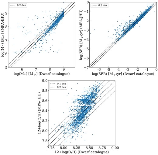
Comparison of properties of the dwarf galaxy catalogue derived from the methods described in Sections 2, 3.2, and 3.1, respectively. (x-axis) and the same properties from the MPA–JHU online archive (y-axis). From left to right, the plots show log(stellar mass), log(SFR(Hα)), and 12 + log(O/H) oxygen abundance. The central bold line is the 1:1 relation and the lighter dashed lines show the 1 and ±0.1/0.2 dex uncertainties.
While our sample and the MPA–JHU sample are not exactly comparable because of the different SDSS data releases and Population Spectral Synthesis methods applied, we note that the stellar masses and SFRs have similar trends and a fraction of the metallicities show differences above 0.2 dex. MPA–JHU results have been estimated from DR7 and DR8 versions of SDSS, both being basically similar, https://wwwmpa.mpa-garching.mpg.de/SDSS/ and https://www.sdss4.org/dr12/spectro/galaxy_mpajhu/. To understand the discrepancy between the MPA–JHU results and our catalogue results, we ran a series of tests to confirm whether this difference originates from using different versions of SDSS or the different ways 12 + log(O/H) is estimated.
To check whether the source data for the MPA–JHU catalogue, has any systematic difference compared to DR-16, we extracted and measured line fluxes for the galaxies in our catalogue from DR-8 and DR-16. In both cases, we used FADO to extract and measure the Hα line fluxes.
As expected, the comparison showed no intrinsic difference between the two data release versions. Our results are in agreement with the ones found by Miranda et al. (2023), where they found that for star-forming galaxies from the SDSS-DR7, the additional modelling of the nebular contribution, using FADO, does not affect the derived fluxes and consequentially the SFR(Hα) and stellar masses.
As seen in Fig. A2, for the dwarf catalogue galaxies, our metallicity estimates differ from the MPA–JHU galaxies’ estimates in a significant fraction of galaxies. To understand this difference we carried a series of tests. We used the flux values from MPA–JHU and applied the calibrator methods applied to our dwarf catalogue. Fig. A3 shows the 12 + log(O/H) derived from both data sets are in good agreement. The important point to note is that both methods of estimating metallicities use line ratios and not absolute fluxes. This implies that the difference in metallicities seen in Fig. A2 likely stems from applying different metallicity calculation methods, rather than a difference in line ratios within the data sets. Fig. A2 also shows the calculated stellar masses of the two samples to be consistent. Stellar masses in our sample have been estimated from SDSS DR-16 photometric data and is thus not influenced by line fluxes or the population spectral synthesis code used.
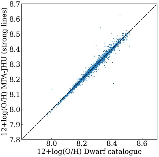
Comparison between 12 + log(O/H) from the dwarf catalogue and from MPA–JHU line fluxes.
APPENDIX B: ONLINE MATERIAL
The full dwarf galaxy catalogue is available online.
