


ABSTRACT
Searches for space–time variations of fundamental constants have entered an era of unprecedented precision. New, high-quality quasar spectra require increasingly refined analytical methods. In this paper, a continuation in a series to establish robust and unbiased methodologies, we explore how convergence criteria in non-linear least-squares optimization impact on quasar absorption system measurements of the fine structure constant α. Given previous claims for high-precision constraints, we critically examine the veracity of a so-called blinding approach, in which α is fixed at the terrestrial value during the model building process, releasing it as a free parameter only after the ‘final’ absorption system kinematic structure has been obtained. We show that this approach results in such small consecutive parameter steps during minimization that convergence is unlikely to be reached, even after as many as 1000 iterations. The fix is straightforward: α must be treated as a free parameter from the earliest possible stages of absorption system model building. The implication of the results presented here is that all previous measurements that have used initially fixed α should be reworked.
1 INTRODUCTION
Searches for space–time variations of fundamental constants are motivated by theoretical expectations, hints in some previous empirical results, and improved technologies, facilities, and procedures. Of particular importance is new instrumentation such as the ESPRESSO spectrograph on the Very Large Telescope (VLT, Pepe et al. 2021) and new laser frequency comb calibration facilities (Steinmetz et al. 2008; Fortier & Baumann 2019; Milaković 2020; Milaković et al. 2020; Probst et al. 2020; Zhao et al. 2021), as well as the forthcoming high-resolution spectrograph ArmazoNes high Dispersion Echelle Spectrograph (ANDES) on the Extremely Large Telescope (ELT, Marconi et al. 2016; Tamai et al. 2018).
Our recent work has focused on measurements of the fine structure constant α in quasar absorption systems, parametrized using Δα/α = (αz − α0)/α0, where the subscripts z and 0 indicate redshift and the terrestrial value, respectively, and where the dimensionless fine structure constant α = e2/4πϵ0ℏc and the dimensional constants in the ratio are expressed in SI units. Our measurements have made use of the non-linear least-squares code, vpfit (Carswell & Webb 2014; Carswell 2023). The vast majority of existing quasar absorption α measurements in the literature have used this code. The vpfit theoretical background and recent enhancements are described in Webb, Carswell & Lee (2021b) and Lee, Webb & Carswell (2022).
To maximize return from new and forthcoming astronomical facilities, it is important to seek improvements, where possible, among all aspects of our current analytical procedures (Webb, Lee & Milaković 2022). In a series of recent papers, we have scrutinized existing methods, identified shortcomings, and have developed more advanced numerical and theoretical procedures. That work includes the application of AI methods to spectral modelling (Bainbridge & Webb 2017a, b; Lee et al. 2021a). Recently, strong bias in some existing quasar absorption measurements has been revealed. The following issues have been found: (i) if data are under- or overfitted (i.e. using too few or too many free parameters), the resulting estimate of Δα/α will be biased. This effect can be minimized by using an appropriate information criterion to decide on the optimal number of model parameters (Webb et al. 2021a). (ii) Model non-uniqueness may occur. The effect is substantially worse if turbulent line broadening is used, rather than compound; turbulent broadening requires many more free parameters to fit the data to compensate for its inability to simultaneously fit profiles having different atomic masses using the same line width, and this in turn biases Δα/α (Lee et al. 2021b). (iii) ‘Distortion blinding’ has been used by some analysts, a procedure that is intended to remove bias but in fact has the opposite effect (Webb et al. 2022; Lee et al. 2023).
One aspect of vpfit that had not previously been studied in any detail concerns convergence, but a number of quite different non-linear least-squares applications motivate doing so. Forbes & Bartholomew-Biggs (2009) suggest that Gauss–Newton (GN) can sometimes exhibit slow convergence and minimize the objective function at each iteration of the process, progressing the GN direction and the negative gradient. Forbes and Bartholomew-Biggs apply their modified GN method to five modelling problems and while they find evidence for improvement, they also find that it is difficult to identify a generalized method for convergence improvement, noting that specific fine-tuning of their method is probably required for any particular highly non-linear problem.
Transtrum & Sethna (2012) suggest that slow convergence and robustness to initial guesses are complementary problems and that methods for improving convergence speed can decrease robustness to initial guesses, and vice versa. Levenberg–Marquardt (LM) algorithms can also be painfully slow to converge when iterations proceed along a narrow canyon (which commonly exists for problems involving a large number of parameters), and suggest several ways in which convergence can be accelerated. One consequence of a flat χ2-parameter space is that algorithms may sometimes push parameters to non-physical (even infinite) values. Transtrum & Sethna (2012) provide an interesting discussion in which they make a distinction between convergence criteria and stopping criteria, and propose a ‘geodesic acceleration’ correction to the LM step, by including second-order corrections in the Taylor approximation of the residuals.
Fratarcangeli et al. (2020) report similar lengthy convergence issues to those we report in this paper. The context of their investigation is image reconstruction. They derive significant speed gains by using LM to locally linearize the problem, decomposing the linear problem into small blocks, using the local Schur complement, obtaining a more compact linear system without loss of information, generality, or accuracy. The other main gain from their work is that the system becomes parallelized and scalable, making it suitable for use with graphics processing units. A process such as this could be explored for vpfit.
In Lee et al. (2023, hereafter L23), we showed that if Δα/α is held fixed at zero while developing the absorption system model, and then subsequently allowed to vary, the final measurement remains locked in a local χ2 minimum near the fixed value, so is likely to bear little or no similarity to the statistically correct solution. In this paper, we develop the L23 analysis further, investigating the impact of non-linear least-squares convergence using vpfit. Stopping criteria must be carefully considered for Δα/α measurements. Previous best-fitting quasar absorption system models have adopted a ‘standard’ practice in terminating iterations; when the change in the goodness of fit between two successive iterations, Δχ2, falls below some ‘reasonable’ threshold, iterations are stopped and the ‘best-fitting’ model obtained. Previous measurements have assumed that final parameter values have been reached in this way. However, if we force algorithms like vpfit to continue iterating well beyond what would normally be considered as a ‘reasonable’ stopping criterion, could the Δα/α solution slowly drift from the previous ‘final’ value, ending up with a significantly different solution? Given the strong bias revealed by the L23 calculations, the question naturally arises as to whether convergence failure issues could also be contributing to systematic errors.
2 ASTRONOMICAL, ATOMIC, AND LABORATORY DATA
The astronomical data used for this study are an isolated section (i.e. flanked by continuum, line-free regions) within an extensive quasar absorption system at zabs = 1.15 towards the quasar HE 0515−4414 (Reimers et al. 1998). Specifically, our study focuses on the lower redshift side the large complex, which we refer to as the ‘left region’. Full details and plots for the left region are described in detail in L23. We use a subsection, rather than the whole absorption system, (a) because the kinematic structure of the left region is such that it provides tight constraints and (b) to make computing times feasible. Recent studies of this absorption system are given by Milaković et al. (2021), Murphy et al. (2022), and L23, and the astronomical (and all other) data used in this paper are exactly the same ESPRESSO data as used in these last two studies.
We opted to use the HE 0515−4414 ESPRESSO data for this study because the analysis carried out in this paper is directly motivated by the different approaches in Murphy et al. (2022) (hereafter referred to as M22) and L23 that use the exact same data. The ESPRESSO spectra were extracted from raw frames by the ESO pipeline data reduction system (Pepe et al. 2021) and combined to form a one-dimensional final spectrum using uves_popler, as described in M22. In M22, as in some previous studies, Δα/α = 0 was fixed throughout model development, and only introduced as a free parameter after a completed absorption system model had been derived. In L23, the same approach was carried out, but with an important addition: as well as fixing Δα/α = 0 throughout model development, three other fixed values were also tried, Δα/α = −10, +10, +30 (all in units of 10−6), for the purpose of demonstrating how the fixed α approach pushes the solution into a false local minimum. In the present analysis, which is an extension of the L23 study, we examine the impact of changing convergence criteria using the same set of four initially fixed Δα/α.
All atomic data, transition oscillator strengths f, damping coefficients Γ, laboratory wavelengths including isotope and hyperfine wavelengths, and sensitivity coefficients q, are as tabulated in the atom.dat file provided with version 12.4 of vpfit (Carswell 2023). All calculations reported in this paper have assumed solar relative isotopic abundances. As pointed out in Webb et al. (1999, 2014), deviations from terrestrial relative isotopic abundances impact significantly on Δα/α. The aim of this paper is not to examine that issue, which has been addressed in a separate study (Webb et al. 2023).
3 OPTIMIZATION METHOD
vpfit v12.4 is used for all calculations in this paper, providing a few improvements over earlier versions. Nevertheless, the results presented here do not depend on the version used – we have checked that our findings are replicated using earlier versions.
In Webb et al. (2021b), we explored different optimization approaches, applied within the vpfit code for modelling high-resolution absorption lines or systems. Prior to version 12.3, the code used both GN and LM algorithms. The two methods differ in the way in which parameter updates are tuned at each iteration during the optimization process, for maximum descent in χ2. In GN optimization, the vector of optimal parameter updates is given by
where γ is a local univariate minimization parameter whose purpose is to minimize the current value of the merit function χ2 at each iteration and |$\boldsymbol {p}_{\mathrm{min}}$| is the vector of parameter updates prior to tuning via univariate minimization.
The LM method takes a different approach. Instead of optimizing the vector of parameter updates, the Hessian matrix is modified at each iteration using a different univariate minimization parameter, η, again to generate the largest reduction in χ2,
where |$\boldsymbol{\mathcal {I}}$| is an identity matrix and η is a positive scalar. Both GN and LM methods are of course very widely used and both work well. Empirically, in the vpfit application, GN sometimes produces the largest χ2 reduction at some iteration, while sometimes LM does. For that reason, vpfit (prior to version 12.3) computes both equations (1) and (2) and selects, at each iteration, the best option. We refer to that approach as GN–LM. However, in version 12.3, an enhancement was introduced: instead of employing one or the other of equations (1) and (2), both minimizations are done at every iteration, the obvious goal being a more efficient χ2 descent. Such a method is evidently neither pure GN nor pure LM, but is a merger of the two approaches, termed ‘hybrid optimization’ in Webb et al. (2021b).
Another relevant vpfit enhancement concerns the way in which the gradient vector and Hessian matrix are calculated; in Webb et al. (2021b) and Lee et al. (2022), we showed how analytical Voigt derivatives avoid problems that occasionally appear using finite difference derivatives and provide better stability in some circumstances. Those changes have been implemented in v12.4.
In all modelling, we imposed an upper limit on the velocity dispersion parameter b ≤ 10 km s−1. In all ai-vpfit models used in this paper, the SpIC information criterion was used (Webb et al. 2021a). This means that the final models in our calculations are all selected to be those for which a minimum value of SpIC is obtained. Also, we have used a Gaussian instrumental profile for convolution with theoretical Voigt profiles (see L23 for details), as did M22.
4 CONVERGENCE TEST USING COMPOUND BROADENING
4.1 100 ai-vpfit compound models
In L23, we computed a total of 400 left region models: 25 independently derived ai-vpfit models for each of four initially fixed Δα/α values, two information criteria (SpIC and AICc), and two line broadening mechanisms (turbulent and compound). In this study, we drop AICc because previous calculations indicate that SpIC is more effective in this context (Webb et al. 2021a). We also drop turbulent broadening, as compound is more general, more physically reasonable, and it incorporates turbulent broadening as a limiting case. Our initial set of calculations in this paper therefore only require 100 models: 25 independently derived ai-vpfit models for each of 4 initially fixed Δα/α settings, using SpIC and compound line broadening. The four initially fixed Δα/α settings are Δα/α = −10, 0, +10, and +30 × 10−6 (in both L23 and this paper). These 100 ai-vpfit models provide the starting point for the longer vpfit iterations described in Section 4.2.
4.2 1000 vpfit iterations for 100 ai-vpfit compound models
Our goal is to examine whether or not the stopping criteria applied in previous measurements result in convergence. The stopping criterion in vpfit is
where the subscript n indicates the nth iteration and
where Nj is the number of data points for the jth transition, the fit being made simultaneously to a total of M transitions. The appropriate choice for Δ in equation (3) clearly depends on the data quality and defines the reliability of the result, as well as the total computing time; if Δ is too large, iterations may terminate too quickly and convergence may not be reached. If Δ is too small, iterations may proceed indefinitely. In all previous α measurements, a balance between these extremes has been attempted, but without sufficiently rigorous checking, hence this study. The vpfit v12.4 default value of Δ, i.e. the hard-coded value used in the absence of user-definition, is 10−3. The Δ values used in the three previous studies of this absorption section are 5 × 10⁻⁴ (Milaković et al. 2021) and 5 × 10⁻⁴ (L23); in both these papers, six additional iterations were carried out after the stopping criterion had been reached), and 2 × 10⁻⁶ (M22, without additional iterations).
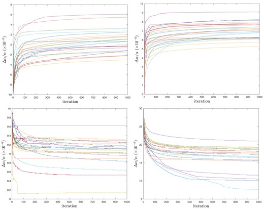
To explore convergence properties, we remove the usual requirement defined by equation (3), and instead force vpfit to iterate 1000 times. Note that while the starting models are already ‘statistically acceptable’ fits to the data (i.e. the reduced χ2 ≈ 1), their Δα/α values are consistently biased towards the starting guesses. Fig. 1 shows the Δα/α convergence tracks for initially fixed Δα/α = −10, 0, +10, +30 × 10−6. These curves reveal a number of interesting properties:
After a small number of vpfit iterations (about 3), each group of 25 models ‘spreads out’ to an approximately constant scatter thereafter.
Each group, on average, gradually drifts away from the starting Δα/α value.
The +30, 0, and −10 samples all drift towards the +10 model, although on average do not quite reach it, even after 1000 iterations. For those three samples, convergence is not reached. For the +10 case, drift is very slow i.e. the data appear close to convergence.
In all four cases studied, the drift rate reduces substantially beyond iteration ∼200–300. This is more easily seen in the linear plots (Appendix A).
In three of the four cases studied, the spread is large compared to the statistical error. But in one case (+10), the behaviour is completely different; both the scatter and the drift are very small and the curves appear stable and consistent.
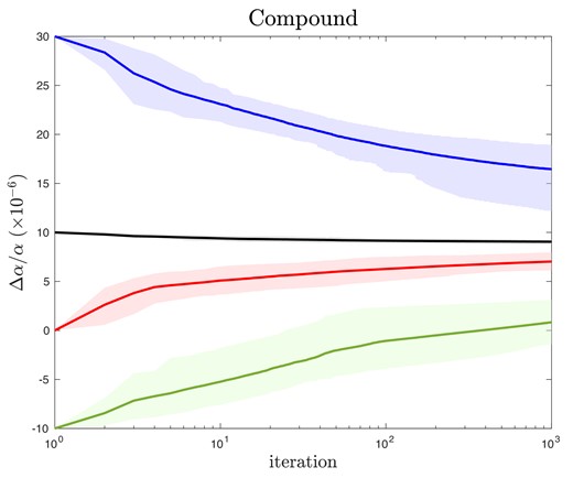
Convergence tracks for four sets of 25 initially fixed Δα/α ai-vpfit models, created using compound broadening. The continuous lines illustrate means over 25 models. Each colour designates a different initially fixed value of Δα/α (equal to the value at iteration 1). All individual curves are shown in Figs A1 and A2. The shaded areas, which illustrate the impact of model non-uniqueness, encompass empirical ±34 per cent ranges. The black (+10) values scatter very little, so the shaded area is not much larger than the line thickness. Δα/α is in units of 10−6. Terrestrial isotopic abundances have been assumed throughout this work. See Section 4.2 for further details.
These results show that initially fixed Δα/α creates long flat ‘canyons’ in χ2–Δα/α space, such that convergence within a reasonable number of iterations is generally unlikely (unless the first guess just happens to coincide with the preferred Δα/α solution). The curves in Fig. 1, whose properties are enumerated above, indicate that the +10 model is preferred over the other cases. The properties of the +10 models also suggest that if so-called blinding is avoided, i.e. Δα/α is a free parameter from the outset of model construction, the convergence failures seen in the +30, 0, and −10 cases will be avoided (simply because if Δα/α is a free parameter throughout model building, its value will already (in this case) be around the +10, iteration 0 value in Fig. 1, and hence will not evolve much subsequently. While these results are derived using one particular absorption system, such that the details would necessarily be different for some other system, there is no reason to expect the more general characteristics found do not apply broadly.
In L23, we showed that solving for Δα/α after being initially fixed, the standard stopping criterion was met relatively quickly, such that relatively few iterations took place, and hence the ‘final’ Δα/α changed little from its starting point. Fig. 2 shows the corresponding Δα/α results for all compound broadening models after 1000 iterations. Comparing initial and final values, a slight reduction in the corresponding statistical (covariance matrix) uncertainties is seen, from (σ+30, σ+10, σ0, σ−10) = (3.20, 1.27, 1.75, 3.73) × 10−6 in L23, to (2.85, 1.21, 1.72, 3.61) × 10−6 here. This is expected because at the starting point, the χ2–Δα/α space is slightly flatter than at the 1000th iteration.

Δα/α measurements for compound broadening models after 1000 iterations plotted against the reduced chi-squared, |$\chi ^2_{\nu } = \chi ^2/\nu$|, where ν is the number of degrees of freedom in the best-fitting model (|$\nu$| is equal to the given number of data points minus the number of free model parameters). The colour coding (designating four different initially fixed values of Δα/α) has the same meaning as in Fig. 1. Δα/α is in units of 10−6. See Section 4.2.
5 CONVERGENCE TEST USING TURBULENT BROADENING
In the M22 study of the zabs = 1.15 absorption system towards the quasar HE 0515−4414, as already explained, fixed Δα/α = 0 was used throughout the vpfit model building process. Δα/α was only allowed to vary freely once the kinematic structure of the absorption system had been established. Once Δα/α is introduced as a free parameter, and all model parameters allowed to vary, the kinematic details evolve a little further, but not much.
5.1 25 ai-vpfit models using turbulent broadening
As shown in L23, extensive ai-vpfit calculations (published after the M22 study) revealed that initially fixed Δα/α creates substantial bias. In light of the various results described above, we emulate the M22 analysis, to see whether we can reproduce (and hence understand) why that measurement does not reflect the ‘correct’ result for that system.1 We therefore carried out an additional set of calculations. For the purposes of illustrating how one can arrive at the M22 Δα/α measurement, the relevant starting models from L23 are the 25 independent ai-vpfit models derived using fixed Δα/α = 0 and turbulent line broadening.
5.2 1000 vpfit iterations for 25 ai-vpfit turbulent models
We can thus use the 25 models described above again as a starting point, evolving them further using vpfit v12.4, allowing 1000 iterations. None of these 25 models (which involved no human decisions in their construction) would be expected to correspond to the M22 manual process specifically. However, the ai-vpfit process [random placement of trial components, as described in Lee et al. (2021a)], together with the Monte Carlo generation of 25 independent models, provides a range of models that are representative of those produced by a human subjective process.
Fig. 3 shows the same general feature as those seen in Fig. 1; the models spread in Δα/α as iterations proceed. After 1000 iterations, the spread is large, and in most cases, convergence does not appear to have been achieved. Interestingly, the compound models appear to reach an approximately constant scatter after only ∼3 iterations, but this requires around 25–30 iterations for the turbulent models.
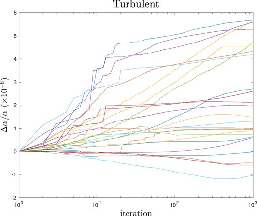
Convergence tracks for 25 initially fixed Δα/α = 0 ai-vpfit models, created using turbulent broadening. Δα/α is in units of 10−6. See Section 5.2.
Fig. 3 raises an obvious question: did the M22 model converge? M22 argue that any residual convergence uncertainty in their model is small compared to the statistical uncertainty. This can easily be explicitly checked by allowing the final M22 model to iterate further. The results of doing this are illustrated in Fig. 4, which clearly shows that, in fact, the M22 model did not achieve convergence. The starting point in this case is Δα/α = 2.15 × 10⁻⁶. It appears to be that the M22 value of 2.15 was reached after 125 vpfit iterations (simply because the Δχ2 stopping criterion used in the M22 study was 10−6, and it is likely that this criterion was not met, such that vpfit is likely to have reached its default maximum of 125 iterations). The result in this case is interesting: as can be seen in Fig. 4, Δα/α continuously increases from its starting point, reaching ∼3.2 by iteration 1000 (a change corresponding to 36 per cent of the M22 statistical uncertainty). Fig. 3 also explains why the M22 result was obtained; the point (125, 2.2) is typical of the 25 models illustrated.
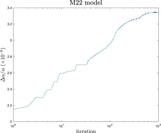
Convergence track for the M22 model, created interactively using turbulent broadening and initially fixed Δα/α = 0. The published measurement is the starting point for 1000 iterations (i.e. ∼2.2), but this gradually evolves to ∼3.3 after 1000 iterations (and may not have reached convergence). Δα/α is in units of 10−6. See Section 5.2.
Fig. 5 shows the Δα/α values reached after 1000 iterations for all 25 turbulent models (blue points) as well as the single M22 model (red point). This plot again illustrates that the M22 result (both Δα/α and |$\chi ^2_{\nu }$|) can easily be reproduced using initially fixed Δα/α and turbulent broadening. See L23 for a detailed discussion on this point, in particular table 1 in that paper, which shows that ai-vpfit derives models with, on average, close to half the number of absorption components compared to M22 (23.1 instead of 41), with a marginally smaller |$\chi ^2_{\nu }$|.

6 SUMMARY AND IMPLICATIONS FOR FINE STRUCTURE CONSTANT MEASUREMENTS
We have carried out a series of ai-vpfit and vpfit calculations, to examine convergence properties when measuring Δα/α in quasar absorption systems. To do so, we focused on one particular, very well studied, system: the left region (as defined in L23) of the zabs = 1.15 towards the quasar HE 0515−4414. No previous studies of convergence issues in this context have been done to our knowledge. The specific goal of our study was to find out how convergence proceeds when ‘blinding’ is used, i.e. imposing an initially fixed Δα/α. Of course, in our conclusions here, we do not criticize blinding methods generically; a comprehensive description of the usefulness of blinding methods used in particle physics, in particular, is provided in Harrison (2002). Nevertheless, we have demonstrated the severe bias that may result if great care is not taken with the way in which a blinding method is applied.
The main result of this work is as follows: when models are developed using fixed Δα/α, it is unlikely that subsequently releasing Δα/α as a free parameter will ever result in convergence, and hence the measurement remains strongly biased towards the fixed value. This kind of ‘blinding’ should not be used in this context, and the parameter Δα/α should be allowed to vary freely in the early stages of model building and left as a free parameter throughout.
The structure of the specific absorption system we have studied here is complex. It is possible that simpler systems, requiring fewer components, may suffer less from the convergence difficulties we have found. None the less, the results derived here provide a strong warning that substantial bias can occur, the clear implication being that any previous measurement that has been derived using initially fixed Δα/α should be reworked. An unbiased reanalysis has now been done for both left and right regions in the zabs = 1.15 system towards HE 0515−4414. A set of ai-vpfit measurements, in which Δα/α is maintained as a free parameter throughout the model building process, is reported in Webb et al. (2023).
ACKNOWLEDGEMENTS
ai-vpfit calculations were carried out using the OzSTAR supercomputer at the Centre for Astrophysics and Supercomputing at Swinburne University of Technology. This research is based on observations collected at the European Southern Observatory under ESO programme 1102.A-0852 (PI: P. Molaro). We thank that team for making their co-added spectrum publicly available. We also thank Dinko Milaković for comments on an early draft of this paper.
DATA AVAILABILITY
The ESPRESSO spectra and associated files used for this analysis are available at https://doi.org/10.5281/zenodo.5512490. The vpfit and ai-vpfit model files are available on request from the authors.
Footnotes
By ‘correct’, we mean a statistically unbiased measurement, in this specific case, based on terrestrial isotopic relative abundances, and using turbulent line broadening.
References
APPENDIX A: FURTHER PLOTS
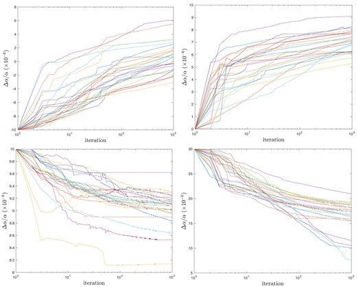
Individual convergence tracks for initially fixed Δα/α for all four compound broadening cases. Δα/α is in units of 10−6.
Same as Fig. A1 except abscissa is linear. Δα/α is in units of 10−6.
