


ABSTRACT
Gaseous nuclear rings are large-scale coherent structures commonly found at the centres of barred galaxies. We propose that they are an accumulation of gas at the inner edge of an extensive gap that forms around the Inner Lindblad Resonance (ILR). The gap initially opens because the bar potential excites strong trailing waves near the ILR, which remove angular momentum from the gas disc and transport the gas inwards. The gap then widens because the bar potential continuously excites trailing waves at the inner edge of the gap, which remove further angular momentum, moving the edge further inwards until it stops at a distance of several wavelengths from the ILR. The gas accumulating at the inner edge of the gap forms the nuclear ring. The speed at which the gap edge moves and its final distance from the ILR strongly depend on the sound speed, explaining the puzzling dependence of the nuclear ring radius on the sound speed in simulations.
1 INTRODUCTION
Gaseous nuclear rings are remarkable structures commonly found at the centres of barred galaxies. They have typical radii of |$50\!-\!1000\, {\rm pc}$| (Comerón et al. 2010), total gas masses of |$10^8\!-\!10^9 \, \rm M_\odot$| (Sheth et al. 2005; Querejeta et al. 2021), and star formation rates spanning a wide range |$0.1\!-\!10\, \rm M_\odot yr^{-1}$| (Mazzuca et al. 2008; Ma, de Grijs & Ho 2018). They are among the most intense star-forming regions of disc galaxies and are considered special laboratories to study star formation under extreme conditions (Moon et al. 2021; Schinnerer et al. 2023). They are sites where galactic outflows can be launched, with profound impact on the evolution of their host galaxies (Veilleux et al. 2020). They constitute cold gas reservoirs for the fuelling of central supermassive black holes. The Milky Way hosts a nuclear ring with a radius of |$R\simeq 120\, {\rm pc}$| that is better known as the Central Molecular Zone (Morris & Serabyn 1996; Henshaw et al. 2023).
It is well-known that nuclear rings are easy to form in simulations (e.g. Athanassoula 1992b; Kim et al. 2012; Sormani, Binney & Magorrian 2015a, and many others). The recipe is simple: let gas flow in a non-axisymmetric rotating barred potential, and a nuclear ring will spontaneously form in the central regions. In the simplest simulations, the gas is assumed to be 2D, isothermal, non-self gravitating, and the barred potential is externally imposed, but a ring can form also if additional physics is included, for example the gas self-gravity, star formation & stellar feedback, live stellar potentials, or magnetic fields (Fux 1999; Armillotta et al. 2019; Tress et al. 2020). However, being able to watch the ring forming in simulations does not mean that we understand the underlying physical process by which it forms, which has remained elusive.
Despite the interest from several astrophysical communities, the physical mechanism by which nuclear rings form is not well understood. What sets the radius of the nuclear ring? What is ‘special’ about its location? Various theories have been proposed, but we argue that they all fail to explain the formation of the rings. These previous theories are reviewed in Section 3.2.
One of the most puzzling aspects is that the radius of the nuclear ring in isothermal simulations of gas flow in a barred potential depends very strongly on the assumed sound speed (e.g. Englmaier & Gerhard 1997; Patsis & Athanassoula 2000; Kim et al. 2012; Sormani, Binney & Magorrian 2015a). For example, doubling the sound speed from |$c_{\rm s}=5\, {\rm km\, s^{-1}}$| to |$10\, {\rm km\, s^{-1}}$| can change the radius of the ring by a factor of two or more (see for example fig. 2 in Sormani, Binney & Magorrian 2015a). This is surprising because the sound speed always amounts to just a small fraction of the orbital speed (typically ∼5 per cent). The flow is always strongly supersonic. None of the currently available theories can explain the strong dependence of the ring radius on the sound speed.
In this paper, we develop a framework to understand the formation of nuclear rings. We propose that the rings are in fact the inner edge of an extensive gap that opens around the Inner Lindblad Resonance (ILR) due to the excitation of waves by a bar potential. These waves remove angular momentum from the gas disc, transporting the gas inwards. The nuclear ring forms due to the accumulation of gas at the inner edge of the gap.
The paper is structured as follows. In Section 2 we present some numerical experiments that illustrate the formation of nuclear rings in simulations. In Section 3 we review the constraints that we believe any plausible theory for the formation of nuclear rings should satisfy, and we review previous theories. In Section 4 we study the excitation of density waves by an external bar potential using linear theory. In Section 5 we illustrate our picture of the formation of the rings. In Section 6 we discuss various connections between this paper and previous works, in particular the works of Goldreich & Tremaine [1978 (hereafter GT78), 1979 (hereafter GT79)] that studied the opening of the Cassini gap in Saturn’s rings. We sum up in Section 7.
2 NUMERICAL EXPERIMENTS
We first perform some numerical experiments by letting non-self-gravitating isothermal gas flow in an external barred potential. This is useful to establish some key points and parameter dependencies that we will need later.
2.1 Numerical setup
We run a total of six 2D non-self-gravitating isothermal simulations of gas flowing in an external barred gravitational potential. The potential is described in Appendix A. Table 1 provides a summary of the simulations run. The equations of motion are
where ρ is the surface density, v is the gas velocity, Φ is the external gravitational potential given by equation (A1) and
is the isothermal equation of state, where cs = constant. We will use values in the range |$c_{\rm s}=1\!-\!20\, {\rm km\, s^{-1}}$|.
Summary of the simulations run in this paper.
| ID | cs | Rmax | Rdisc | NR |
|---|---|---|---|---|
| [|$\, {\rm km\, s^{-1}}$|] | [ kpc] | [ kpc] | ||
| 01 | 1 | 1.5 | 1.2 | 512 |
| 02 | 2.5 | 1.5 | 1.2 | 512 |
| 03 | 5 | 1.5 | 1.2 | 512 |
| 04 | 10 | 1.5 | 1.2 | 512 |
| 05 | 20 | 1.5 | 1.2 | 512 |
| 04_Large | 10 | 5.0 | 5.0 | 740 |
| ID | cs | Rmax | Rdisc | NR |
|---|---|---|---|---|
| [|$\, {\rm km\, s^{-1}}$|] | [ kpc] | [ kpc] | ||
| 01 | 1 | 1.5 | 1.2 | 512 |
| 02 | 2.5 | 1.5 | 1.2 | 512 |
| 03 | 5 | 1.5 | 1.2 | 512 |
| 04 | 10 | 1.5 | 1.2 | 512 |
| 05 | 20 | 1.5 | 1.2 | 512 |
| 04_Large | 10 | 5.0 | 5.0 | 740 |
The parameters are defined in Section 2.
We solve equations (1) and (2) using the public grid code pluto (Mignone et al. 2007) on a 2D static polar grid in the region |$R \times \theta = [0.1 \, {\rm kpc}, R_{\rm max}] \times [0, 2\pi ]$|. The grid is logarithmically spaced in R and uniformly spaced in θ with NR × 1024 cells. The resolution along the R direction is approximately ΔR = 0.00529 R, i.e. we have a resolution of |$\Delta R=0.529\, {\rm pc}$| at the inner boundary of |$R=100\, {\rm pc}$|. The number of cells in each direction is chosen so that the aspect ratio of the cells is approximately Δθ(R/ΔR) ∼ 1. We use the following parameters: rk2 time-stepping, no dimensional splitting, hll Riemann solver and the default flux limiter. We solve the equations in the frame rotating at Ωp by using the rotating_frame = yes switch. Boundary conditions are outflow both on the inner boundary at |$R=0.1\, {\rm kpc}$| and on the outer boundary at R = Rmax.
The initial density distribution is
Note that, since the equations of motion (1) and (2) are invariant under density rescaling, the density units are arbitrary. The quantity |$\bar{\rho }$| therefore essentially sets the density units, and without loss of generality we set |$\bar{\rho }=1$|. The quantity |$\rho _\epsilon =10^{-12}\bar{\rho }$| corresponds to the density floor imposed in the simulation to avoid crashing. We introduce the bar gradually to reduce transients (e.g. Athanassoula 1992b). We start with gas in equilibrium on circular orbits in the logarithmic axisymmetric potential Φ0 and then linearly turn on the non-axisymmetric part of the potential Φ1 during the first |$313\, {\rm Myr}$|.
2.2 Disc with initial radius smaller than the ILR
Simulations 01–05 investigate the evolution of a uniform gas disc with an initial radius |$R_{\rm disc}=1.2\, {\rm kpc}$| that is smaller than |$R_{\rm ILR}=1.61\, {\rm kpc}$| (Appendix A). The only difference between these five simulations is the assumed sound speed (Table 1). Fig. 1 shows the surface density as a function of time.
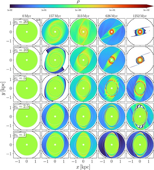
Surface density of simulations 01–05 (see Table 1), illustrating the formation of nuclear rings for various values of the sound speed cs. The only difference between these simulations is the assumed cs. Time increases from left to right. Sound speed decreases from top to bottom (top row is the 05 simulation, bottom row is the 01 simulation). The black dashed circle indicates the Inner Lindblad Resonance. The thin dotted circle indicates the instantaneous ring radius according to the definition used in Fig. 3. All panels are rotated so that the major axis of the bar potential (i.e. the θ = 0 line in equation A1) coincides with the x axis. The sense of rotation is clockwise. Trailing density waves excited by the bar potential are visible (see in particular the second and third column from the left). The radius of the ring at the end of the simulation (rightmost column) strongly depends on the sound speed. Regions with densities ρ < 10−2 are shown white.
As soon as the bar potential is turned on, trailing spiral waves are excited. These waves are clearly visible at |$t=157 \, {\rm Myr}$| and |$t=313 \, {\rm Myr}$|. The movies of the surface density as a function of time show that the waves are first excited at the outer edge of the disc, and propagate inwards. We will confirm later in Sections 4.3.4 and 4.3.5 using linear analysis that sharp edges are indeed regions where strong wave excitation takes place, and therefore play a key role in the formation of the rings. The wiggles that are visible along the spirals in some panels (for example the panel at |$t=313\, {\rm Myr}$| and |$c_{\rm s}=10\, {\rm km\, s^{-1}}$|) are due to the wiggle instability (Wada & Koda 2004; Kim, Kim & Kim 2014; Sormani et al. 2017; Mandowara et al. 2022).
Fig. 2 plots a cut through the x axis of Fig. 1 at |$t=157\, {\rm Myr}$|. The radial wavelength increases with increasing sound speed. This will be explained by the dispersion relation derived below (equation 54). The amplitude of the waves decreases inward, despite the prediction of the linear analysis according to which the amplitude of density waves should increase inward due to geometric effects (see Section 4). The reason for this behaviour is that the waves in the simulations become quickly non-linear and develop shocks. The shocks cause the waves to dissipate, decreasing their amplitude and depositing their (negative) angular momentum into the gas disc. As we will argue in Section 5, this process is what decreases the angular momentum of the gas disc and causes it to shrink.
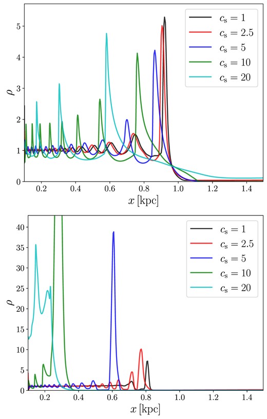
Surface density on the x axis for simulations 01–05 at |$t=157\, {\rm Myr}$| (top) and and |$t=1252\, {\rm Myr}$| (bottom). In other words, these are horizontal cuts in the second column and fifth column of Fig. 1. The oscillations are the density waves excited by the bar potential. The wavelength of the waves increases with increasing sound speed cs. The waves are highly non-linear.
The final size of the ring depends very strongly on the sound speed (rightmost column in Fig. 1). This is further quantified in Fig. 3, which shows the evolution of the ring size as a function of sound speed. As can be seen in the bottom panel, increasing the sound speed by a factor of two can change the final ring size by the same factor.
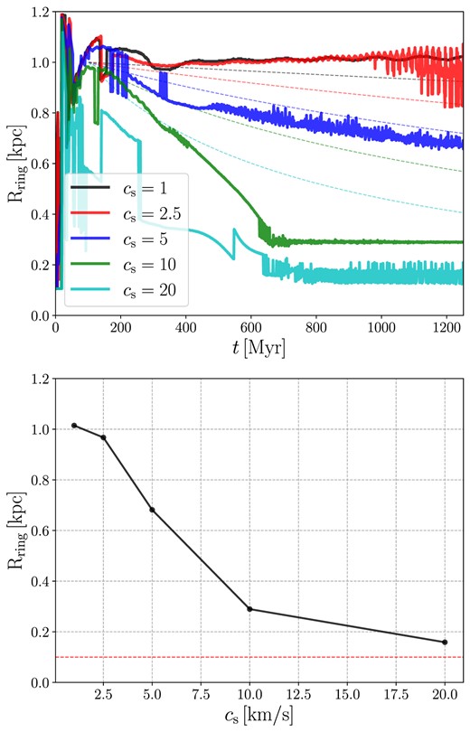
Top: The full lines show the radius of the ring as a function of time in the simulations 01–05. The radius of the ring is calculated as |$R_{\rm ring}=\sqrt{R_x R_y}$|, where Rx and Ry are the locations of the density maxima along the x- and y-axis respectively. The dashed lines show the prediction according to equation (76) obtained in the linear approximation (see Section 5.2). Bottom: The radius of the ring mediated over simulation time |$t=1152\!-\!1252\, {\rm Myr}$| as a function of the sound speed. The radius strongly depends on the sound speed. The horizontal dashed line indicates the inner boundary of the computational grid.
2.3 Disc with initial radius larger than the ILR
Simulations 04 and 04_Large only differ in the size of the initial gas disc, |$R_{\rm disc}=1.2\, {\rm kpc}$| versus |$R_{\rm disc}=5\, {\rm kpc}$|. Thus, simulation 04 includes only the flow inside the ILR (|$R_{\rm ILR}=1.61\, {\rm kpc})$|, while simulation 04_Large comprises the large-scale flow in the entire bar region.
Fig. 4 shows that the final ring size is approximately the same in both simulations, and therefore that ring size does not depend on the large-scale flow outside the ILR. This implies that the mechanism determining the radius of the ring must be ‘local’ (see point 5 in Section 3.1).
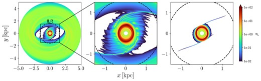
Surface density of the 04_Large (left and zoom-in panel) and 04 (right) simulation at the end of the simulation (|$t=1252\, {\rm Myr}$|). The only difference between the two simulations is that in simulation 04_Large the initial gas disc extends to |$R_{\rm max}=5.0\, {\rm kpc}$|, while in simulation 04 only to |$R_{\rm disc}=1.2\, {\rm kpc}$|. Simulation 04 is the same as shown in the second row of Fig. 1. The dashed circle indicates the ILR. All panels are rotated so that the major axis of the bar potential (i.e. the θ = 0 line in equation A1) coincides with the x axis. The sense of rotation is clockwise. Comparison between the two simulations shows that the ring always reaches the same final size, regardless of the larger-scale flow outside the ILR, demonstrating that the physical process determining the radius of the ring must be ‘local’.
Fig. 5 illustrates the evolution of the axisymmetrized surface density as a function of radius in the simulation 04_Large. In particular, we can see that an extensive gap of low surface density is opened around the ILR. The nuclear ring is the inner edge of this gap, where the material that once was in the gap has accumulated.
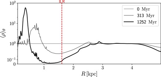
Axisymmetrized surface density 〈ρ〉θ = ∫ρ(R, θ)dθ/(2π) as a function of cylindrical radius R for the simulation 04_Large at three different times. An extensive gap opens around the ILR. The material that once was in the gap is transported inwards and accumulates at the inner edge of the gap, forming a nuclear ring.
3 PREVIOUS THEORIES AND WHAT WE LOOK FOR IN A THEORY
3.1 Conditions that a plausible theory must satisfy
We introduce the conditions that we believe any plausible theory for the formation of nuclear rings must satisfy. We take the approach that numerical experiments, such as those in Section 2, guide us on how the ring properties should depend on the underlying parameters. We summarize the insights obtained from simulations into the following five conditions:
The radius of the ring must depend on the circular rotation curve. Athanassoula (1992b) and Li, Shen & Kim (2015) have shown that the radius of the ring in simulations changes if we change the circular velocity curve of the underlying gravitational potential, i.e. if we change the axisymmetric part of the gravitational potential (see in particular fig. 4 in Li, Shen & Kim 2015), while keeping everything else fixed.
The radius of the ring must depend on the non-axisymmetric part of the underlying potential. Sormani, Binney & Magorrian (2015b) has shown that the radius of the ring can change significantly if we change the quadrupole of the potential while keeping the monopole (and therefore the rotation curve) fixed. Hence, a theory aiming to explain why rings form at a certain location must take into account a dependence on the non-axisymmetric part of the potential.
The radius of the ring must depend on the bar pattern speed. Many authors (e.g. Athanassoula 1992b; Li, Shen & Kim 2015; Sormani, Binney & Magorrian 2015b, among others) have shown that the radius of the ring depends on the rotation speed of the bar.
The radius of the ring must depend on the equation of state of the gas. Many authors (e.g. Englmaier & Gerhard 1997; Patsis & Athanassoula 2000; Kim et al. 2012; Sormani, Binney & Magorrian 2015a, among many others) have shown that the size of the ring strongly depends on the sound speed. This is confirmed by the numerical experiments we conducted in Section 2.2 (see in particular Figs 1 and 3). Thus, the radius of the ring does not depend solely on the gravitational potential but must involve the equation of state of the gas.
The radius of the ring must be determined ‘locally’, i.e. the final ring size should not depend on the larger-scale flow at R > RILR. This is demonstrated by the numerical experiments in Fig. 4, which shows two simulations that differ only for the extent of the simulated gas disc. The 04_Large simulation (left) covers the entire ‘bar region’, out to |$R_{\rm disc}=5\, {\rm kpc}$|. It includes the usual bar-driven accretion flow from the disc to the ring. The 04 simulation (right) is the same shown in the second row of Fig. 1, and it only simulates a gas disc of |$R_{\rm disc}=1.2\, {\rm kpc}$|, which is all contained within the ILR at |$R_{\rm ILR}=1.61 \, {\rm kpc}$| (Fig. A1). The final size of the ring is essentially the same in the two simulations (it is slightly larger in the 04_Large simulation because fresh gas is continuously brought from outside the ILR, which takes longer to lose angular momentum). This shows that removal of angular momentum also happens in the vicinity of the ring. Material from outside the ILR that crosses the ILR continually loses angular momentum up to when it settles on the ring.
3.2 Previous theories for the formation of nuclear rings
Here we briefly summarize previous theories for the formation of the ring and for determining its location. We argue that none of them provides a satisfactory explanation for the formation of the rings by showing that each of them fails to satisfy at least one of the conditions outlined in Section 3.1.
The resonant theory (Combes 1988; Buta & Combes 1996; Combes 1996). This is perhaps the most widely accepted theory, especially in the extragalactic community. It states that the ring forms at the Lindblad resonance under the continuous action of gravity torques from the bar potential.
|$\boldsymbol{\times }$| Refutation: This theory satisfies conditions 1, 3, 5, and if the notion of ILR is generalized to include strongly barred potentials (van Albada & Sanders 1982; Athanassoula 1992a), it may satisfy condition 2. However, since the position of the resonance does not depend on the equation of state of the gas, it does not satisfy condition 4. Moreover, the numerical experiments shown in Fig. 1 show that the radius of the ring forms at a radius R that is much smaller than |$R_{\rm ILR}=1.61\, {\rm kpc}$| (on this point, see also Regan & Teuben 2003).
The minimum shear theory (Lesch et al. 1990; Krumholz & Kruijssen 2015). This theory states that the ring forms at the radius at which the shear, as calculated from the axisymmetric rotation curve, is minimum. This conclusion stems from an analogy with accretion disc theory, in which transport is more efficient where shear is higher, so gas is expected to pile up and form a ring at the point of minimum shear.
|$\boldsymbol{\times }$| Refutation: This theory satisfies conditions 1 and 5, but does not satisfy conditions 2, 3, 4. Sormani & Li (2020) demonstrate in detail that simulations are inconsistent with this theory.
The reverse shear theory (Sormani et al. 2018b). This theory states that the ring forms in a region where a family of non-axisymmetric closed periodic orbits called x2 orbits displays ‘reverse shear’ that prevents viscous spreading, making it possible to confine a stable ring.
|$\boldsymbol{\times }$| Refutation: This theory satisfies conditions 1, 2, 3, and 5, but it does not satisfy condition 4 since it predicts that the radius of the ring depends exclusively on the gravitational potential.
In conclusion, none of the currently available theories satisfies all the criteria introduced in Section 3.1, highlighting the need for a new theory.
4 LINEAR DISC DYNAMICS
The simulations in Section 2 suggest that density waves are important for the removal of angular momentum of the disc and the opening of the gap. To gain insight into this process, in this section we study the excitation of waves by the bar potential in the linear regime, and estimate the amount of angular momentum that they remove from the gas disc as a function of the unperturbed density profile ρ0 and of the sound speed cs. As we shall see, the excitation of waves happens primarily at two locations: (i) near the ILR. This regime has been studied in detail by GT79, and we will not repeat their calculations here; (ii) at sharp edges (i.e. strong gradients) in the unperturbed density distribution ρ0. The insight gained in this section will be used in Section 5 to develop a new picture for the formation of nuclear rings.
Consider a 2D axisymmetric differentially rotating fluid disc in equilibrium in an external gravitational potential. Our goal is to study the propagation of small perturbations (waves) and their excitation by a ‘small’ external potential. These ‘density waves’ are conceptually similar to sound waves in air, but the rotation makes the dynamics richer and mathematically more complex. In Appendix B we present a 1D toy problem that can be solved fully analytically and provides a mathematically simpler analogue to the more complicated problem studied in this section.
We start from the disc’s unperturbed steady state and linearize the equations of motions around it. We ignore the self-gravity of the gas. The equations of motion are the continuity and Euler equations,
where ρ is the surface density, |$\mathbf {v}=v_x \hat{{\bf e}}_x+ v_y \hat{{\bf e}}_y$| is the velocity, P is the pressure, and Φ(x, t) is the external gravitational potential. We assume a polytropic equation of state
where γ ≥ 1 and K is a constant. To simplify the calculations it is convenient to introduce the enthalpy h defined by
substituting (7) into (8) and integrating we find
Using (8), the equations of motion (5) and (6) can be expanded in polar coordinates (R, θ) as
4.1 Unperturbed state
We assume that the density, velocity and gravitational potential of the unperturbed steady-state are
Substituting these into (10)–(12) and assuming steady-state and axisymmetry (|$\partial _t = \partial _\theta = 0$|), we see that the continuity equation (10) and the azimuthal Euler equation (12) are already satisfied, while the radial Euler equation (11) gives
In the following, h0, Φ0 and Ω are prescribed functions of R that satisfy equation (17). Note that given Φ0(R), there formally exists an equilibrium solution h0(R) for any arbitrary rotation profile Ω(R). However, not all possible profiles are physical. To avoid instability, the unperturbed state must satisfy the Rayleigh stability criterion, which states that a necessary and sufficient condition for the local axisymmetric stability of an inviscid differentially rotating fluid disc is that the specific angular momentum monotonically increases with R, i.e.1
In this paper we will assume mainly two types of density profiles. The first is a constant density profile
The second is a truncated disc profile, i.e. a density that is roughly constant at R ≪ Redge, has a relatively sharp transition at an edge Redge during which it drops at a much lower value, and is then roughly constant again at R > Redge. Note that the edge cannot be made too thin, otherwise it would violate the Rayleigh criterion (18). When later in the paper it will be necessary to assume a specific truncated profile for numerical calculations, we will use the following:
where
where Redge is the position of the edge and ΔR controls its width. The quantity |$\bar{\rho }$| is a constant that, as noted in Section 2.1, essentially defines the units used for density. Physically meaningful results do not depend on the particular value of this quantity since the equations of motion (5) and (6) are invariant under density rescaling. Without loss of generality, we set |$\bar{\rho }=1$|.
4.2 Linearized equations
To study the propagation of small waves on top of the unperturbed state described in the previous section, we expand all quantities as
Substituting equations (22)–(25) into equations (10)–(12) and linearizing by keeping only first-order terms in the quantities with subscript 1, we obtain
where we have defined the convective derivative of the unperturbed state
and the Oort parameter
Without loss of generality, we can write all the ‘small’ subscript-1 quantities as
where |$\tilde{\rho }_1$|, |$\tilde{v}_{1R}$| etc. are complex, and the ‘physical’ quantity is the real part. The general solution of equations (26)–(28) can always be decomposed in such modes because the equations are linear and the superposition principle applies. Each mode evolves independently from the others in the linear approximation. In this paper, we will only be concerned with m = 2 as this is the only non-zero term in the expansion of the external potential described in Appendix A. Hereafter, we drop the |$\, \tilde{}\,$| symbol to avoid cluttering. With these substitutions, we have |$\partial _t = -i \omega$| and |$\partial _\theta =i m$|. Substituting equation (31) into (9) we have
where we have introduced the sound speed of the unperturbed medium
Equation (36) is valid for γ ≥ 1 (including equality). We also define
This is the angular frequency with which each mode appears to rotate, as can be understood by noting that
In this paper, we will always take Ωp to be the same as the pattern speed of the bar described in Appendix A, since only modes at this frequency can be excited by the external potential in the linear approximation.
Substituting (31)–(35) into (26)–(28) we obtain
Isolating vR1 and vθ1 from (41) and (42) we find
where we have defined
The points where D = 0 define the Lindblad resonances,2 while the point where Ω = Ωp defines the Corotation resonance. Now we can substitute (43) and (44) into (40) and use (36) to eliminate ρ1 to obtain an equation in the variable h1:
where
Equation (47) coincides with equation (13) of GT79. The same equation has been also derived by others (e.g. Feldman & Lin 1973; Bertin et al. 1989). It is a second order ordinary differential equation with non-constant coefficients H(R) and W(R). The term F(R) is a forcing term (recall that Φ1(R) is externally prescribed). Note that H(R) and W(R) diverge where (Ω − Ωp) = 0 and where D = 0, i.e. at the corotation and Lindblad resonances.
In order to eliminate the first order derivative from equation (47), it is convenient to define a new variable g1 such that
Substituting equation (52) into equation (47), one finds
where
Equation (53) is the fundamental equation that governs linear modes in the disc. It is similar to equation (B10) in the toy problem in Appendix B, but is more complicated because K is not constant. To follow the calculations in the following section more easily, it is useful to note that equation (53) is equivalent to that of a forced harmonic oscillator, |$m \ddot{x} + k^2(t) x = q(t)$|, where t replaces R, m is the mass, k(t) is a time-dependent spring constant, and q(t) is a time-dependent external force.
4.3 Analysis of equation (53)
Equation (53) describes the dynamics of the most general linear perturbation in the presence of an external potential. To calculate the amplitude of waves excited by the bar potential we need to solve this equation with appropriate boundary conditions. Unfortunately, no general analytic solution is available, so we need to resort to various approximations that are valid in different radial ranges. Fig. 6 provides an overview of the various regimes that we analyse.
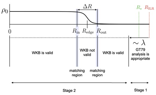
Schematic diagram of where the various approximate solutions of equation (53) apply. ‘WKB is valid’ denotes where the general solution of equation (53) is well approximated as the sum of the WKB solution (56) and the equilibrium solution gQ given by (60). ‘WKB not valid’ denotes the region near the edge where equation (67) is more appropriate. The shaded ‘matching regions’ denote where both solutions are simultaneously valid and we can apply the method of matched asymptotic expansions. The region within approximately one wavelength λ from the ILR is where the analysis of GT79 is appropriate. ‘Stage 1’ and ‘Stage 2’ denote the regions corresponding to the two stages in our picture of the formation of the rings described in Section 5.
This section is structured as follows. In Section 4.3.1 we identify special points where the treatment of equation (53) require special care because the coefficient K either vanishes or diverges. In Section 4.3.2 we derive the WKB solution of the homogeneous equation associated with (53), and show that it is generally very accurate away from the special points and away from sharp edges (see Fig. 6). In Section 4.3.3 we derive a particular solution of the non-homogeneous (53) that is approximately valid when cs is sufficiently low and away from special points and sharp edges. In Section 4.3.4 we obtain exact numerical solutions of equation (53) in a few selected cases, to illustrate that truncated discs with sharp edges excite much stronger waves than uniform discs. In Section 4.3.5 we present an approximated analytical solution of equation (53) that is valid near sharp edges and estimate the flux of angular momentum at sharp edges.
4.3.1 Special points
There are two types of points where equation (53) requires special attention:
Turning points. These are the points R⋆ where K(R⋆) = 0. At these points, the character of the solutions changes from oscillatory to exponential.
Singular points. These are points where K(R) diverges. As can be seen from equations (54) and (48)–(51), this happens at the Lindblad and Corotation resonances.
Fig. 7 shows the coefficients of equation (53) for a uniform and a truncated disc profile in the case |$c_{\rm s}=10\, {\rm km\, s^{-1}}$|. In the region of interest for this paper there is typically one turning point R⋆ and one singular point at RILR, with R⋆ < RILR. As we shall see below, R⋆ is where the medium becomes absorbing and leading waves incident from R < R⋆ are reflected into trailing waves that subsequently travel inwards. The position of R⋆ depends on both the sound speed cs and the shape of the unperturbed density profile ρ0(R). In the limit cs → 0 we have R⋆ → RILR. However, for a finite value of the sound speed, the two points are distinct.
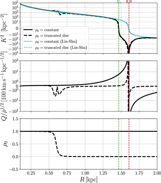
Top: The coefficient K(R) in equation (53) for a uniform disc (full black line) and a truncated disc (dashed black line) in the case |$c_{\rm s}=10\, {\rm km\, s^{-1}}$|. In the WKB approximation, this represents the wavenumber versus radius of free density waves that rotate with the same pattern speed of the bar (see Section 4.3.2). The cyan lines compare with the wavenumber given by the Lin-Shu dispersion relation (59). Middle: The forcing term Q(R) in equation (53). Bottom: The uniform (ρ0 = 1) and truncated disc (equation (20) with |$R_{\rm edge}=0.6\, {\rm kpc}$| and |$\Delta R = 0.03\, {\rm kpc}$|) density profiles assumed in this figure. The red vertical dashed line marks the ILR. The green vertical dashed line marks R⋆, which is defined as the radius where K(R) = 0 (see Section 4.3.1).
4.3.2 WKB solution of the homogeneous equation
Consider the homogeneous equation associated with equation (53), i.e. the equation obtained setting Q = 0. This equation describes the propagation of ‘free’ density waves on top of the unperturbed disc in the absence of the external bar potential. In this case, equation (53) is of the same form of equation (C1) and it can be solved in the WKB approximation. The general solution is given by equation (C9), which adapted to the notation used here reads
where C1 and C2 are arbitrary complex constants and R0 is an arbitrary radius.
The two terms on the right-hand side of equation (56) represent two waves travelling in opposite directions, analogously to the two sound waves that are possible in a uniform medium at a given frequency (see Appendix B). The quantity K is the wavenumber, which varies with radius. When K2 > 0, the solution (56) has oscillatory character and waves can travel, while when K2 < 0 it has exponential character and the medium is absorbing. Thus, as can be seen from Fig. 7, travelling waves can exist only at R < R⋆. Equation (54) implicitly contains ω, and therefore for fixed R this expression can be seen as a dispersion relation K = K(ω).
The direction of propagation of the waves can be understood from the group velocity. In Appendix D we calculate the group velocity of the WKB waves and we find that trailing waves (C1 ≠ 0 and C2 = 0) propagate inwards, while leading waves (C1 = 0 and C2 ≠ 0) propagate outwards.
The angular momentum flux associated with the WKB waves (56) is calculated in Appendix E and is given by equation (E10),
Since C1 and C2 are constant for a given WKB wave, this equation shows that the flux of angular momentum is constant as a function of R. It can be shown that the angular momentum flux corresponds to the adiabatic invariant associated with the general WKB solution (C9). Equation (57) also shows that the trailing wave has FA > 0, while the leading wave has FA < 0. Thus, trailing (leading) wave packets remove (increase) the amount of angular momentum in the region where they travel.
What is the range of validity of the WKB approximation? The WKB approximation is expected to work well when the following parameter is small (see equation C3):
Fig. 8 shows that the WKB approximation works exceptionally well at R < R⋆, but breaks down near R = R⋆. The WKB approximation will also fail near sharp edges, because dK/dR becomes large (e.g. Fig. 7).
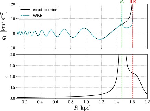
Top: Comparison between the exact solution of equation (53) and the WKB approximation. The full black line shows the solution obtained numerically integrating equation (53) from |$R=0.1\, {\rm kpc}$| with initial conditions g1 = 1, dg1/dR = 0 (full black line). The cyan dashed line shows the WKB approximation (56). We assumed |$c_{\rm s}=10\, {\rm km\, s^{-1}}$| and constant unperturbed density ρ0(R) = 1. Bottom: The ‘small’ parameter of the WKB approximation (equation 58). At R⋆ it diverges. The WKB approximation works well only at R < R⋆.
The WKB approximation used here is not completely equivalent to the more well-known Lin-Shu approximation. The Lin-Shu dispersion relation in the absence of self-gravity (G = 0) is given by (equation 6.55 of Binney & Tremaine 2008)
where D is given by equation (45). The top panel in Fig. 7 compares the Lin-Shu dispersion relation (cyan line) with the dispersion relation given by equation (54). The two are similar at R < R⋆, but differ considerably around R⋆ and RILR. In particular, in the Lin-Shu approximation the turning point (which is the point where waves are absorbed) coincides with the ILR, while it is at a smaller radius (R⋆) according to equation (54). This is because the Lin-Shu dispersion relation assumes very small sound speed, while the dispersion relation (54) takes into account the effect of finite sound speed. Indeed, in the limit of vanishing sound speed we recover the Lin-Shu dispersion relation from our dispersion relation (54). This can be shown by noting that in this limit |$W(R) \simeq -D/c_{\rm s}^2$| (equation 49), while H2 ≪ W and dH/dR ≪ W (equation 54).
4.3.3 Approximate non-oscillatory solution of the non-homogeneous equation
An approximate particular solution of equation (53) is
In the analogy with the harmonic oscillator, this solution corresponds to following the ‘instantaneous’ equilibrium position of the oscillator as the external force slowly varies. It is expected to be valid when the ‘force’ Q(R) varies slowly enough compared to the frequency of the harmonic oscillator. More formally, one can substitute g1 = gQ in equation (53), and impose that the first term on the left-hand side is small, i.e. d2g1/dR2 ≪ K2g1. This gives the following condition:
This condition is verified in particular at low sound speed, since K → ∞ as cs → 0 at fixed R (see equation 54).Equation (60) is equivalent to equation (15) of GT79. It is a non-wave solution which is the analogue of the black dashed solution for the toy problem in Fig. B1 in Appendix B.
4.3.4 Excitation of density waves in uniform and truncated discs
We numerically solve equation (53) in a few selected cases. The goal is to calculate the amplitude of density waves excited by the bar potential in a region [R1, R2] where R1 < R2 < R⋆, to illustrate how the amplitude depends on cs and on the unperturbed density profile ρ0. A sharp edge might be present inside [R1, R2]. The appropriate boundary conditions are ‘radiation’ boundary conditions (see Fig. 9). Causality requires that waves propagate away from the region [R1, R2], because a solution in which waves come towards it would require a source of waves outside this region. Therefore, the correct solution to our problem contains waves propagating inwards at R = R1, and outwards at R = R2. These are schematically shown as the two waves W1 and W2 in Fig. 9. The goal is to calculate the amplitude of W1 and W2.
![Schematic diagram of excitation of waves in the region [R1, R2]. W1 and W2 are the waves excited by the barred potential in this region. Arrows indicate the direction of propagation. See Section 4.3.4 for more details.](https://oup.silverchair-cdn.com/oup/backfile/Content_public/Journal/mnras/528/4/10.1093_mnras_stae082/1/m_stae082fig9.jpeg?Expires=1750198016&Signature=hUwBPyPK4kT3jebQnsszus~MjuQXQ-paDFzkWV9We3ABTbAQyqmFHTzfxdX3Mxa6dc-1cIQpakGTc6uounk1SJYSJrXHqOgjKViE~7cK-gloPYYBDM9OCmmuiJgwXick3j2uaNy1x3UEU8ifPeTy~euG8Uzp8OenrqoWR73gWZC6vkFCqPoXl4LR0q3U-jl6qPKVnLfxfeypxJ1KDAkFy0SLdHg9o~PI5s2pBRSGbFaYO1VD7GgQhGfriUpUwkNJ6kMsxwEpciFunH22OLFMs~MahRfKL8NGLIou5t9zQuuVEsD36MrgNn62OqpIavQtpDclsiEYTZU~WS7xZ1lfGA__&Key-Pair-Id=APKAIE5G5CRDK6RD3PGA)
Schematic diagram of excitation of waves in the region [R1, R2]. W1 and W2 are the waves excited by the barred potential in this region. Arrows indicate the direction of propagation. See Section 4.3.4 for more details.
Although the numerical solutions of equation (53) described in these section are exact, to impose the boundary conditions we need to use the results of the WKB analysis as we need to identify the direction of propagation of the waves. We proceed as follows. Let g1 be an exact solution of equation (53) that satisfies the radiation boundary condition. We assume that at R1 and R2 the conditions (58) and (61) are valid, so in a neighbourhood of these points we can decompose the solution as the sum of the WKB solution (56) and of the ‘equilibrium’ solution (60). Therefore in a neighbourhood of R1 we can write
and in a neighbourhood of R2
where W1 and W2 are trailing and leading WKB waves respectively (equation 56),
To find C1 and C2, we use the shooting method. We start from R = R1 with an initial guess for C1 (which is a complex number, so the guess involves two real numbers) and initial conditions given by equation (62), and integrate until R2. At R2 we decompose g1 − gQ into its WKB components. This decomposition is unique and can be found by equating g1 − gQ and d(g1 − gQ)/dR with equation (56) and its derivative and solving the resulting algebraic system of two equations in the two unknowns that give the amplitude of the two waves. We then vary the initial guess for C1 until the solution at R2 only contains an outgoing wave. The amplitude of the latter gives C2.
Fig. 10 shows the result of this procedure applied to [R1, R2] = [0.1, 1.0] for a uniform (left) and truncated disc profile (right), and for two different values of the sound speed. The truncated disc profile is chosen so that the width of the edge is comparable to the wavelength (λ = 2π/K) at the edge. The edge cannot be much smaller than this without violating the Rayleigh criterion (Section 4.1). The top panel shows the solution g1, the middle panel the corresponding density profiles, and the bottom panel the flux of angular momentum associated with the waves W1 and W2 obtained performing the WKB decomposition as a function of R. The amplitude of the excited waves is given by the oscillations around the equilibrium solution gQ (dashed line).
![Waves excited by the bar potential in the region $[R_1,R_2]=[0.1,1.0]\, {\rm kpc}$ in uniform and truncated discs in the linear approximation. Waves excited in uniform discs are small, while waves excited at the sharp edge of a truncated disc are much larger. For each of the four cases shown, the three panels from top to bottom display the following. Top: The solution of equation (53) with radiation boundary conditions at $R=0.1\, {\rm kpc}$ and $R=1.0\, {\rm kpc}$ (full black line), and the approximate ‘instantaneous equilibrium’ solution gQ given by equation (60) (dashed black line). The oscillations of g1 around gQ give the amplitude of the excited waves. Middle: The thin full black line shows the unperturbed density profile ρ0, which can be either a uniform disc (ρ0 = 1) or a truncated disc given by equation (20) with $R_{\rm edge}=0.6\, {\rm kpc}$ and $\Delta R=0.03\, {\rm kpc}$ (for $c_{\rm s}=10\, {\rm km\, s^{-1}}$) or $\Delta R=0.003\, {\rm kpc}$ (for $c_{\rm s}=1\, {\rm km\, s^{-1}}$). The dashed and full thick black lines show the total density (unperturbed + perturbation) that corresponds to the solutions g1 and gQ shown in the top panel. Bottom: The flux of angular momentum associated to the two WKB waves into which g1 − gQ can be decomposed. See Section 4.3.4 for more details.](https://oup.silverchair-cdn.com/oup/backfile/Content_public/Journal/mnras/528/4/10.1093_mnras_stae082/1/m_stae082fig10.jpeg?Expires=1750198016&Signature=W-WkVhyaJzIYsUyLwESbhp3V9AczmSBFPGp8H5mk6pTvcjtIwcvWzVBhA5UClRx3XvKEe7c~uEFtCeIlDTjvNYbJ7GOtB9doU4hFNGmXQmRUvVOwJIeLXdm06fs37BgOBkXFXp6RKLN6wcYeYTvGupYVy2nlAqUexni1XqgBAucUHItjcmXLfwzBZbPjn8gJ1vhhmOVXZdeXWJjSgY6jUvJvtT6N2P45GpvgiAE8e6f-x~Vo3VrXZrjc4D0Fh5UAj7wqsTUzGxf9TKa2iHO2la2CtpSVMGo67760KHdJOs-cQhXDjvbmhOisNl1HEJbkBmVSYfqE7LIa3Q8yN6Ccng__&Key-Pair-Id=APKAIE5G5CRDK6RD3PGA)
Waves excited by the bar potential in the region |$[R_1,R_2]=[0.1,1.0]\, {\rm kpc}$| in uniform and truncated discs in the linear approximation. Waves excited in uniform discs are small, while waves excited at the sharp edge of a truncated disc are much larger. For each of the four cases shown, the three panels from top to bottom display the following. Top: The solution of equation (53) with radiation boundary conditions at |$R=0.1\, {\rm kpc}$| and |$R=1.0\, {\rm kpc}$| (full black line), and the approximate ‘instantaneous equilibrium’ solution gQ given by equation (60) (dashed black line). The oscillations of g1 around gQ give the amplitude of the excited waves. Middle: The thin full black line shows the unperturbed density profile ρ0, which can be either a uniform disc (ρ0 = 1) or a truncated disc given by equation (20) with |$R_{\rm edge}=0.6\, {\rm kpc}$| and |$\Delta R=0.03\, {\rm kpc}$| (for |$c_{\rm s}=10\, {\rm km\, s^{-1}}$|) or |$\Delta R=0.003\, {\rm kpc}$| (for |$c_{\rm s}=1\, {\rm km\, s^{-1}}$|). The dashed and full thick black lines show the total density (unperturbed + perturbation) that corresponds to the solutions g1 and gQ shown in the top panel. Bottom: The flux of angular momentum associated to the two WKB waves into which g1 − gQ can be decomposed. See Section 4.3.4 for more details.
The figure illustrates the following points:
Waves excited in uniform discs are weak (right panels). The amplitude is essentially zero at |$c_{\rm s}=1\, {\rm km\, s^{-1}}$|, while it is small but visible at |$c_{\rm s}=10\, {\rm km\, s^{-1}}$|. This reflects the fact that the approximate solution gQ is very accurate at low sound speed, but is less accurate when the sound speed is slightly larger. Physically, the reason why stronger waves are excited for larger cs is that the wavelength λ of WKB increases with cs (Fig. 11), so that waves couple more effectively to the forcing term Q which varies on large scales. As we shall see in Section 5, waves excited in uniform discs are too weak to remove the angular momentum necessary to open the gap.
Waves excited at the edge of a truncated disc are strong (left panels). The total density becomes negative near the edge (ρ1 + ρ0 < 0), indicating that the linear approximation breaks down. The waves become highly non-linear and in reality they will develop shocks very quickly near the edge, as indeed seen in the simulations of Section 2. The amplitude of the waves is similar at |$c_{\rm s}=1\, {\rm km\, s^{-1}}$| and |$c_{\rm s}=10\, {\rm km\, s^{-1}}$|, but the flux of angular momentum is much larger for |$c_{\rm s}=10\, {\rm km\, s^{-1}}$|. This will be explained by equation (72) below.
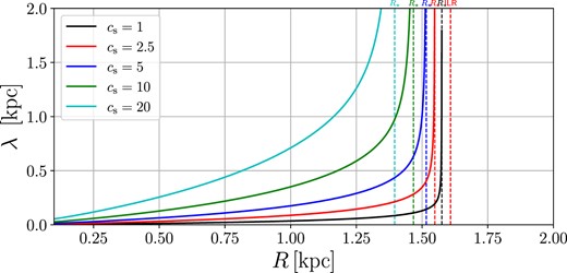
Wavelength of WKB waves (λ = 2π/K) for different values of the sound speed cs. The wavenumber K is given by equation (54) assuming a uniform disc ρ0(R) = 1.
There is a simple explanation for why strong waves are excited at sharp edges. When the background density ρ0(R) varies rapidly, such as at the edge of a disc, the forcing term Q(R) on the right-hand side of equation (53) will have a localized bump on the same scale (see dashed line in the middle panel of Fig. 7). This localized bump acts like an impulsive force. In the analogy with the harmonic oscillator, this force will impart a finite amount of ‘momentum’ equal to the integral of the force. The amplitude of the resulting oscillations gives the amplitude of the waves excited at the edge.
4.3.5 Analytical estimate of the waves excited at the edge of a truncated disc
In this section, we derive an analytical estimate for the amplitude of waves excited at a sharp edges.
Consider an edge at Redge of width Rout − Rin = ΔR, where Rin and Rout > Rin are the two extremities of the region over which the edge extends (see Fig. 6). The shape of the edge can be arbitrary. The edge is assumed to be thin but not too thin, otherwise the unperturbed density profile would violate the Rayleigh criterion (18) and become unstable. In practice, considering the Lin-Shu approximation (equation 59) this means that the edge should not be thinner than approximately one wavelength, λ = 2π/K.
Away from the edge and from turning and singular points,, i.e. at R < Rin and Rout < R < R⋆, the general solution of equation (53) can be approximated as the sum of the WKB solution (56) and of the particular solution (60). We assume that waves are excited only near the edge, i.e. at Rin < R < Rout. We impose radiation boundary conditions, so that at R < Rin we have only the trailing wave and at R > Rout only the leading wave. Therefore outside the edge we write
The constants Cin and Cout will be determined by solving equation (53) near the edge and matching the two solutions.
Near the edge, the forcing term Q varies rapidly, violating condition (61), and the equilibrium solution (60) fails (dashed line in the middle panel of Fig. 7). To solve equation (53) near the edge, we proceed as follows. We assume that K is approximately constant across the edge, i.e. in the range Rin < R < Rout. This is justified by our assumption that the edge is relatively sharp (see also the black dashed line in the top panel of Fig. 7). Under this assumption, equation (53) can be solved using the method of variation of parameters. The general solution is
where K ≃ K(Rin) ≃ K(Rout). The constants A1 and A2 are determined by the condition that the solution contains only waves travelling inwards at radii R < Rin, and waves travelling outwards at radii Rout < R. These calculations are reported in Appendix F1. We find
where Qout = Q(Rout) and Qin = Q(Rin).
Both equations (66) and (67) are valid solutions of equation (53) in a neighbourhood of Rin and in a neighbourhood of Rout (shaded regions in Fig. 6). Matching these two solutions gives (see Appendix F1):
The coefficients Cin and Cout give the amplitude of density waves excited at the edge. It can be shown that the absolute values |Cin| and |Cout| are independent of R0, as they should since the angular momentum flux at the edge should be independent of this arbitrary radius.
The rapid variation of Q near the edge is what generates density waves. The coupling between the forcing term Q and the density waves is expected to be maximum when the scale-length over which Q varies is comparable to the wavelength of the waves λ = 2π/K (similarly to the toy problem in Appendix B), i.e. when ΔR ≃ λ.
We can use equations (57) and (70) to calculate the angular momentum flux carried by the waves excited at the edge. To obtain a closed formula it is necessary to make some further assumptions on the edge. If the edge of the disc is marginally stable to the Rayleigh criterion (18), one has |Rout − Rin| ∼ cs/Ω ∼ 1/K. This is the sharpest edge that can be constructed without making the unperturbed density distribution unstable. Then the exponential exp (− iKs) in the integral of equation (70) is nearly constant. As shown in Appendix F2, in this case equation (70) reduces to
Note that this is essentially the impulse approximation, i.e. we have assumed that the force Q gives an instantaneous ‘kick’ at R = Redge. Using equation (E10), the flux of angular momentum of waves excited at a sharp edge is then
Equation (72) is correct when the distance of the edge from the ILR is larger than approximately one wavelength, i.e. K|Redge − RILR| ≫ 1. At |Redge − RILR| = λ/(2π2) = 1/(πK) and approximating D(R) ≃ (R − RILR)(dD/dR), as appropriate near the ILR where D vanishes, equation (72) becomes identical to equation (46) of GT79 which gives the flux of angular momentum of waves excited at the resonance.
5 THE FORMATION OF NUCLEAR RINGS
We are now ready to put everything together and describe our picture of the formation of nuclear rings. For simplicity, we illustrate our scenario by starting from a uniform density distribution that extends from R = 0 to R ≫ RILR. This is essentially the same situation as in simulation 04_Large shown (Fig. 5 and Section 2.3). The formation of the ring can be schematically divided into two stages, which depend on the distance of the edge of the gas disc from the ILR. The regions corresponding to the two stages are marked in Fig. 6. The simulations 01–05 shown in Fig. 1 only include the second stage.
5.1 First stage (|Redge − RILR| ≲ λ)
In the first stage, a trailing spiral wave is excited near the ILR by the external bar potential. This is the regime analysed by GT79. The wave travels inwards but for realistic strengths of the bar potential it very quickly becomes non-linear and develops into a shock. The wave then dissipates, depositing its (negative) angular momentum into the gas disc (i.e. removing angular momentum from the gas disc).3 This reduces the angular momentum of the disc, causing the gas to move inward. A gap opens around the ILR.
The width of the gap opened in the first stage is the range of validity of the calculations of GT79, which is approximately one wavelength, i.e. |Redge − RILR| ∼ λ, where λ = 2π/K. Using the Lin-Shu approximation (equation 59) and approximating D ≃ (R − RILR)(dD/dR) (recall that D = 0 at the resonance) we have λ ∼ cs/|D|1/2 ∼ cs/|(Redge − RILR)(dD/dR)|1/2 and therefore |$|R_{\rm edge}-R_{\rm ILR}|\sim |c_{\rm s}^2/(\mathrm{d}D/\mathrm{d}R)|^{1/3}\sim (c_{\rm s}/v_0)^{2/3}R_{\rm ILR}$|. The size of the gap is therefore much smaller than the radius of the resonance, and increases for increasing sound speed.
The velocity at which the edge of the gap moves can be estimated by dividing the flux of angular momentum of the waves, FA, by the amount of angular momentum per unit radius in the unperturbed disc, 2πρ0R3Ω,
The angular momentum flux FA during the first stage can be estimated using equation (46) of GT79, bearing in mind that these calculations are valid in the linear approximation and should not be expected to be too accurate for the highly non-linear waves excited by a strong bar potential considered here. Taking into account that m = 2, we find
Inserting the numbers of our gravitational potential (Appendix A) into equation (74) we obtain |$\mathrm{d}R_{\rm edge}/\mathrm{d}t\simeq 6\, {\rm km\, s^{-1}}$|. The duration of the first stage can be estimated by dividing the size of the gap by the velocity of the edge. Using |Redge − RILR| ∼ (cs/v0)2/3RILR, |$v_0=220\, {\rm km\, s^{-1}}$|, |$R_{\rm ILR}=1.6\, {\rm kpc}$| and the value of dRedge/dt found above we obtain
This time is relatively short compared to the total timescales involved (see Fig. 3). In reality, the evolution is likely to be even faster than equation (75) suggests because of the non-linearity of the process. The evolution of the gap after the first stage and its final size are determined by the second stage.
5.2 Second stage (|Redge − RILR| ≳ λ)
At the beginning of the second stage there is a gap around the ILR, and the distance between the inner edge of the gap and the ILR is approximately one wavelength. Since the width of the edge at this point can be at most one wavelength (because the edge tail cannot extend beyond the ILR), the edge is ‘sharp’ by definition and strong waves will be excited at its location according to the analysis in Section 4.3. Similarly to the waves excited near the ILR in the first stage, the waves excited near the edge will become quickly non linear and dissipate, removing the angular momentum from the gas disc and causing the edge to move inwards. Gas will accumulate at the edge, forming a ring.
This process can be seen in action in Figs 1 and 2. The first figure shows trailing waves excited by the bar potential (see for example |$t=157\, {\rm Myr}$|). The pitch angle of these waves is in good agreement with that predicted by the WKB analysis of Section 4.3.2, indicating that these are indeed trailing waves of the same type studied in the linear analysis. Fig. 2 shows that the amplitude of the waves decreases inwards, contrary to what would be predicted in the linear approximation (e.g. Fig. 10). This is because when the waves become strongly non-linear and develop shocks, they quickly dissipate and decrease their amplitude. This dissipation is what allows the wave to deposit their angular momentum into the gas disc.
The speed at which the edge moves during the second stage can be estimated using equation (73), where we use equation (72) to estimate the flux of angular momentum FA of waves excited at sharp edges. Using the Lin-Shu approximation (equation 59) to write K ≃ |D|1/2/cs, and m = 2, we find
where the factor of 2 takes into account that the outward-travelling leading wave excited at the edge will be reflected at R = R⋆ into an inward-travelling trailing wave. Note that equations (74) and (76) only differ for the factor in the first round parentheses on the right-hand-sides, and this factor coincides in the two equations at a distance of approximately one wavelength from the ILR. This is the point where we transition from the analysis of GT79 to the analysis in Section 4.3.5, and from the first to the second stage.
Fig. 3 compares the size of the ring as a function of time predicted by equation (76) to that measured in the numerical experiments of Section 2.2. We find that the equation captures the general trends in the figure, including the fact that the edge moves faster for larger sound speed, but it tends to underestimate the speed at which it moves, especially at large sound speed. That the analytic prediction is not quantitatively accurate is not surprising considering that equation (76) is derived in the linear approximation, but the waves excited at the edge are strongly non-linear (Figs 2 and 10). The flux of angular momentum generated in the case of a uniform disc is too small to move the edge significantly over the course of several Gyr (Fig. 10).
When does the edge stop moving? The process above continues until waves can be effectively excited at the edge, which happens when both of the following conditions are satisfied: (i) the edge is ‘sharp’, i.e. the edge width is smaller than a few times the wavelength of density waves λ = 2π/K; (ii) the gravitational potential Φ1 is sufficiently strong. The distance between the edge and the ILR poses an upper limit to the width of the edge since the edge cannot cross the ILR, ΔR < |RILR − Redge|.4 Therefore, when the edge is not sufficiently far from the ILR, it must be sharp. In particular, we can expect the edge to keep moving until it is located a few wavelengths away from the ILR. Since λ increases linearly with cs (equation 59 and Fig. 11), we expect the edge to move farther at larger sound speed, which explains why the ring radius depends on the sound speed.
Predicting exactly where the edge will stop, and therefore the final radius of the ring, is a difficult task. The process is highly non-linear, and the unperturbed density profile changes in a way that cannot be calculated in the linear approximation. Empirically, we find from the numerical experiments in Section 2 that for our assumed gravitational potential the ring stops when one can fit approximately seven wavelengths λ between Redge and RILR. For weaker barred potential, the edge might stop sooner if Φ1 is too small to generate sufficient flux of angular momentum at the edge.
Finally, we note that our theory satisfies all the five conditions that we laid out in Section 3.1. Conditions 1–3 are satisfied because clearly the radius of the ring depends on the rotation curve, on the non-axisymmetric part of the gravitational potential, and on the pattern speed of the bar which sets the location of the ILR. All these dependencies are also evident in equation (76). Condition 4 is satisfied because the radius of the ring depends on the sound speed of the gas in two ways: first because the speed at which the edge moves away from the ILR increases as a function of cs (see equation 76), and second because the final ring size is determined by the condition that the edge should be a few wavelengths away from the ILR, which results in smaller rings at larger sound speed since as discussed above the wavelength increases with the sound speed. Condition 5 is satisfied since the excitation of density waves at the edge is a local process.
6 DISCUSSION
6.1 Comparison with the works of Goldreich & Tremaine
During the late 70’s and early 80’s, Peter Goldreich and Scott Tremaine published a series of papers in which they studied the dynamics of planetary rings. The calculations and physical processes studied in these works have much in common with those presented in the present paper. Here we highlight the main similarities and differences between them and the present paper.
GT78 developed a picture for the formation of the Cassini division in Saturn’s ring that has several similarities with our picture for the formation of nuclear rings described in Section 5. In both cases: (i) a gap opens near the Lindblad resonance due to waves excited at the resonance; (ii) subsequent excitation of waves at the edge of the gap continues to widen the gap. The main differences are: (i) The bar potential considered here is a perturbation many orders of magnitude stronger than the one from Saturn’s satellite Mimas; (ii) the sound speed is negligibly small in Saturn’s problem, while the effects of finite sound speed are important in our problem (Section 5); (iii) self-gravity is negligible for our case, but it is not negligible in Saturn’s problem. In particular, gravity is the main means of transport of angular momentum in Saturn’s problem, while advective transport through pressure is the main mechanism for transport in our problem.
GT79 studied the excitation of density waves in a differentially rotating gas disc by a rigidly rotating external potential. Their calculations have similarities with those presented in Section 4, but there are three key differences: (i) GT79 assume that cs → 0, while we take into account the effects of finite sound speed; (ii) GT79 assume that ρ0 varies slowly; (iii) GT79 included the self-gravity of the gas disc, which we have neglected. The combination of (i) and (ii) is why GT79 find that waves can be excited only at the resonances, while for example in Section 4.3.4 we find waves excited away from the resonance. The physical explanation is the following. The external potential can couple effectively to density waves only when the wavelength of WKB waves (λ = 2π/K) is comparable to the typical scalelength over which the forcing term Q in equation (53) varies, i.e. when λ ∼ Q/(dQ/dR). The quantity Q/(dQ/dR) is determined by the external potential Φ1 and by the unperturbed density distribution ρ0, and is therefore typically very large unless there are sharp edges in ρ0. In the limit of vanishing sound speed, Q/(dQ/dR) ≫ λ everywhere except near the turning point R⋆ at which λ → ∞ (see Fig. 11). In the limit cs → 0 the turning point merges with the ILR (Section 4.3.1) and λ is small everywhere else. Thus, in this limit waves can be excited only at the resonance. For finite sound speed instead λ can become large and comparable to Q/(dQ/dR) away from the resonance and waves can be excited (see Fig. 11). As we have seen in Section 5, the effects of finite sound are important in the formation of nuclear rings.
6.2 Relation to x2 orbits
Several works have suggested a connection between nuclear ring and x2 orbits (e.g. Regan & Teuben 2003; Li, Shen & Kim 2015; Sormani et al. 2018b). The x2 orbits are a family of non-circular closed orbits that can exist in the central regions of a bar potential, and are elongated in the direction perpendicular to the major axis of the bar (e.g. Contopoulos & Grosbol 1989; Athanassoula 1992a). Fig. 12 illustrates the relation between these orbits and the present paper. The streamlines of the ‘equilibrium’ solution equation (60) are very similar to closed x2 orbits in the same bar potential. Therefore, the WKB waves excited by the bar potential that we studied in Section 4.3 travel on top of an x2 gas disc. Our picture for the formation of the rings is therefore consistent with the idea that gas in nuclear rings flows on x2 orbits.
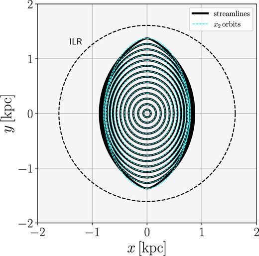
Black full lines: Streamlines of the non-wave solution (60) in the case cs → 0 and constant ρ0. Cyan dashed lines: Ballistic closed x2 orbits in the barred potential described in Appendix A. The two are similar, showing that the density waves excited by the bar potential discussed in Section 4 are essentially perturbations travelling on top of an x2 disc.
6.3 Relation with the resonant theory
Our theory is somewhat the ‘opposite’ of the resonant theory, which states that the ring forms at the ILR (Combes 1988, 1996; Buta & Combes 1996). In our theory the gas is pushed away from the ILR rather than accumulating at it. Our theory is more consistent with the fact that the rings are typically inside the ILR in simulations (e.g. Englmaier & Gerhard 1997; Patsis & Athanassoula 2000; Kim et al. 2012; Li, Shen & Kim 2015; Sormani, Binney & Magorrian 2015a) and with observations that show that for example in the Milky Way the radius of the nuclear ring is ≃ 100–200 pc while the ILR is at |$R\gt 500\, {\rm pc}$| (Henshaw et al. 2023). A key difference between our theory and all previous theories, including the resonant theory, is that we can explain the puzzling dependence of nuclear ring size on the sound speed seen in simulations.
6.4 Brief considerations on magnetic fields and turbulent pressure
The mechanism for the formation of rings described in Section 5 relies on waves propagated through pressure. We would therefore expect that adding magnetic fields, which create magnetic pressure in the gas, could have a similar effect as increasing the sound speed, and would therefore lead to smaller rings.
Turbulent pressure seems to have a smaller effect than ‘real’ microscopic pressure on the size of nuclear rings. Salas, Naoz & Morris (2020) performed some numerical experiments with external turbulence driving. Their figs 1 and 2 show that turbulence driving changes the size of the nuclear ring by a smaller amount than an increase in the sound speed when the injected turbulent energy is comparable to the corresponding increase in thermal energy. We attribute this to the fact that, due to the presence of inelastic collisions, in a gas with turbulent pressure sound waves do not propagate as efficiently as in a gas that has the same amount of microscopic pressure.
6.5 On the assumption of an isothermal equation of state
Throughout this work, we have assumed an isothermal equation of state. This follows a tradition of works adopting the isothermal prescription to study the dynamics of the interstellar medium (ISM) on galactic scales and in nuclear rings (e.g. Roberts 1969; Cowie 1980; Athanassoula 1992b; Englmaier & Gerhard 1997; Fux 1999; Maciejewski 2004; Kim et al. 2012; Sormani, Binney & Magorrian 2015a; Fragkoudi, Athanassoula & Bosma 2017; Li et al. 2022). However, the real ISM is multiphase, turbulent, and highly inhomogeneous. It is therefore natural to ask whether the isothermal prescription can capture the basic mechanism for the formation of nuclear rings.
Numerical simulations that include a multiphase medium via thermal instabilities (Sormani et al. 2018a) as well as gas self-gravity, star formation, and supernova feedback (Armillotta et al. 2019; Tress et al. 2020) show that the large-scale morphology of nuclear rings is only moderately affected by the presence of this additional physics. The main differences are observed at small scales (smaller or comparable to the width of the rings), where gas condenses into molecular clouds and collapses to make star formation. The large-scale properties of the ring, such as its radius and width, can be often mimicked by using an ‘effective’ isothermal sound speed. For example, we found that the morphology, width, and radius of the nuclear ring in the simulations of Sormani et al. (2018a), which include a non-equilibrium chemical network that produces a two-phase medium via the thermal instability, are very similar to those obtained by replacing the non-equilibrium network and the associated cooling function with an isothermal equation of state with a low sound speed of |$c_{\rm s}\simeq 1\, {\rm km\, s^{-1}}$|. This low value is because the gas in the ring is very cold in these simulations, as they did not include any sources of heating or turbulence such as stellar feedback. When star formation and stellar feedback are added to the simulations (e.g. Armillotta et al. 2019; Tress et al. 2020), they heat up the gas and generate turbulent pressure, and the morphology of the rings can still be crudely mimicked by raising the isothermal sound speed (although as noted in Section 6.4 by less than the turbulent velocity dispersion, which would be the naive way of doing it). Similarly, the effects of magnetic fields can be crudely mimicked by increasing the sound speed by summing in quadrature the typical Alfvén speed.
In conclusion, the isothermal prescription should be viewed as an ‘effective’ equation of state that takes into account in a phenomenological way the additional physics via a single parameter that can be easily controlled. Ultimately, the key property that needs to be captured in this approach is the ability of the medium to propagate waves through pressure. Thus, the sound speed does not correspond to the actual kinetic temperature of the gas, but to an ‘effective’ temperature that takes into account in a crude way averaging over different phases, turbulent motions on unresolved scales, and other effects such as magnetic pressure. Reassuringly, numerical simulations suggest that the basic mechanism for the formation of the ring is well captured using this approach.
7 CONCLUSION
We have used both hydrodynamical simulations and analytical calculations of linear disc dynamics to construct a new theory for the formation of nuclear rings in barred galaxies. According to this theory, nuclear rings are an accumulation of gas at the inner edge of a gap that forms around the ILR of a bar potential. The gap initially opens because the bar potential excites strong trailing waves around the ILR, which remove angular momentum from the gas disc and push the gas inwards. The gap then continues to widen because the bar potential excites trailing waves at the inner edge of the gap, until the edge stops at a distance of several wavelengths from the ILR. The gas accumulates at the inner edge of the gap, forming a ring. The speed at which the gap edge moves and its final distance from the ILR, which determine the radius of the nuclear ring, depend on the gas sound speed through the dispersion relation.
Our theory has much in common with the picture for the formation of the Cassini gap in Saturn’s ring proposed by GT78. The most important differences are that (i) the effects of finite sound speed are important in our problem, while the sound speed can be assumed to be vanishingly small in the planetary problem; (ii) we have neglected the effects of self-gravity, which are typically less important in the nuclear ring problem, but cannot be neglected in the planetary rings problem.
ACKNOWLEDGEMENTS
MCS acknowledges financial support of the Royal Society (URF\R1\221118). ES acknowledges financial support of the European Union’s Horizon 2020 research and innovation program under the Marie Skłodowska-Curie Grant agreement No. 101061217. JLS acknowledges financial support of the Royal Society (URF\R1\191555).
DATA AVAILABILITY
The data and code underlying this article will be shared on reasonable request to the authors.
Footnotes
Linear waves of small amplitude travel to the centre without affecting the unperturbed density of the disc. It is only when they become non-linear that they can dump their angular momentum in the unperturbed disc.
Recall also that as discussed in Section 4.3.5 the edge cannot be too thin, otherwise the system becomes Rayleigh-unstable. Thus, we expect the edge width to remain of order λ during the shrinking process.
The divergence theorem states that for any vector-valued function F(x):
References
APPENDIX A: EXTERNAL GRAVITATIONAL POTENTIAL
In Appendix A, we describe the external barred gravitational potential that is used throughout the paper. Consider a rigidly rotating potential of the following form:
where (R, θ) are standard polar coordinates. This represents the simplest possible barred potential, consisting of a monopole and a quadrupole. For the monopole, we take a simple axisymmetric logarithmic potential,
where |$v_0=220\, {\rm km\, s^{-1}}$| and |$R_{\rm c}=0.05\, {\rm kpc}$|. The logarithmic potential is convenient because the rotation curve is rising at small R and is flat at R ≫ Rc, roughly consistent with the rotation curves observed in many disc galaxies (e.g. Lang et al. 2020). For the quadrupole, we employ the analytic density-potential pair described in appendix A of Sormani et al. (2018b),
where A = 0.4 is a dimensionless parameter that quantifies the bar strength, e = 2.71[…] is Euler’s number, |$v_0=220\, {\rm km\, s^{-1}}$| is the same as in equation (A2), |$R_q=1.5\, {\rm kpc}$| is the radial scalelength, and f is the following function:
where E1(x) is the exponential integral function, a special function defined as
This quadrupole reproduces well those generated by N-body exponential bars. We assume that the potential rotates with pattern speed |$\Omega _{\rm p}=40 \, {\rm km\, s^{-1}}\, {\rm kpc}^{-1}$|. This places the ILR at |$R_{\rm ILR}=1.61 \, \, {\rm kpc}$|, the corotation resonance at |$R=5.5\, {\rm kpc}$|, and the outer Lindblad resonance at |$R_{\rm OLR}=9.39\, \, {\rm kpc}$|. Fig. A1 shows the circular velocity (top), the resonance diagram (middle) and the quadrupole (bottom) of our potential.
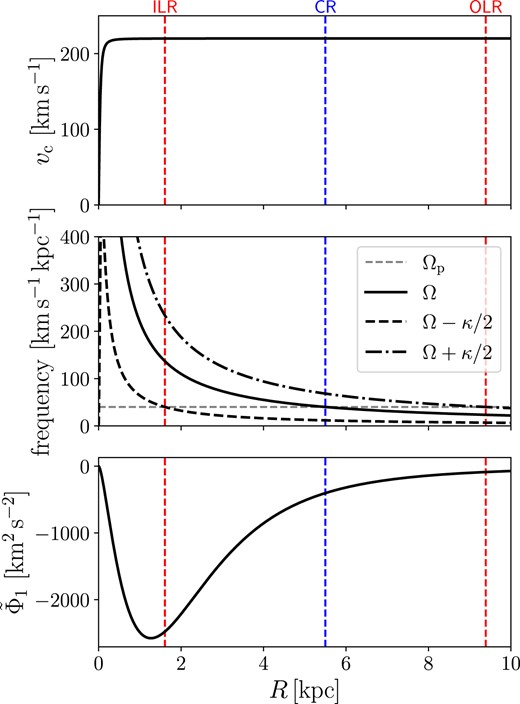
Top: The circular velocity of our potential, vc = (rdΦ0/dR)1/2. Middle: The curves Ω and Ω ± κ/2, where Ω = vc/R and κ is the epyciclic frequency (equation 46). The intersection of these curves with the horizontal line at Ωp gives the position of the resonances, indicated by vertical dashed lines. Bottom: The quadrupole (equation A3).
APPENDIX B: EXCITATION OF 1D WAVES BY AN OSCILLATING GAUSSIAN POTENTIAL (TOY MODEL)
In Appendix B, we describe a toy model that shares various similarities with the actual problem studied in the main text but has the advantage that it can be solved fully analytically. This toy model is helpful for understanding why the amplitude of the waves excited by an external potential can depend very strongly on the gas sound speed.
We can draw the following correspondences between this toy problem and the problem studied in the main text (i) 1D sound waves correspond to spiral density waves, and in particular to the WKB waves discussed in Section 4.3.2 (ii) the 1D Gaussian potential corresponds to the bar potential; (iii) the linear momentum of plane waves plays a similar role to the angular momentum of the spiral density waves; (iv) equation (B7) is the analogue of equation (53).
B1 Statement of the problem
Consider a 1D isothermal fluid at rest with uniform density ρ0. Our goal is to study the waves excited in this medium by a ‘small’ time-varying external potential Φ(x, t).
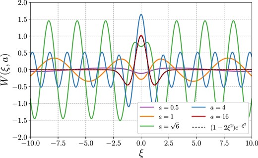
The function W(ξ, a) defined by equation (B15) for various values of a.
The equations of motion of this system are the same as equations (1), (2), and (3) where the gradient is replaced by d/dx since the problem is one dimensional. We linearize these equations around the background state by writing ρ(x, t) = ρ0 + ρ1(x, t) and v(x, t) = v1(x, t) and keeping only the first-order terms in the quantities with subscript 1. We obtain
Without loss of generality, we can write all variables as
where |$\tilde{F}$| are complex quantities. We use complex notation for mathematical convenience, but it is understood that the physical quantities are given by the real part. Substituting all perturbation variables in the form (B3) into (B1) and (B2), and omitting the symbol |$\, \tilde{}\,$| hereafter for simplicity of notation, we obtain
Isolating v1 from (B5) and introducing the variable s1 = ρ1/ρ0 we have
Substituting (B6) into (B4) we obtain an ODE for s1:
where
Equation (B7) is the equation of a forced harmonic oscillator. Now consider an oscillating Gaussian potential of the form
where Φ1 is the strength of the potential, x0 is the width of the Gaussian perturbation, ω0 is the oscillation frequency. Since in the linear approximation there is no coupling between modes at different frequencies, only modes with frequency ω = ω0 will be excited by this potential. Hence we assume ω = ω0 hereafter. Introducing the dimensionless coordinate ξ = x/x0 and using (B9), equation (B7) becomes
where
and we have introduced the following dimensionless parameters
The parameter a is the inverse of the sound speed, normalized with the typical scale-length and frequency of the problem. The parameter b is the normalized strength of the external potential.
B2 Analytical solution
The general solution of equation (B10) is
where C1 and C2 are arbitrary constants and
Here, |$\operatorname{erf}(z) = \frac{2}{\sqrt{\pi }} \int _0^z e^{-t^2} \, \mathrm{d}t$| is the error function, which is defined for complex argument z (to evaluate the integral, you can choose any integration path in the complex plane that leads to z). Note however that the functions X and W are real because the erf function has the properties |$\operatorname{erf}(\overline{z}) = \overline{ \operatorname{erf}(z)}$| and |$\operatorname{erf}(-z) = \operatorname{erf}(z)$|, where the bar denotes the complex conjugate.
Fig. B1 plots the function W(ξ, a) for various values of a. In the limit ξ → ±∞ we have that |$\operatorname{erf}(\xi + i c/2) \rightarrow \pm 1$| for any fixed c, so W(ξ, a) → ∓iα[eiaξ − e−iaξ]. Therefore W(ξ, a) becomes a plane wave when ξ → ±∞ (as one would expect). In the limit a → ∞ the W tends to the forcing term K on the right-hand-side of equation (B1).
What is the amplitude of the waves that are excited by the external potential (B9)? In order to answer this question we have to determine the constants C1 and C2 in equation (B14) by imposing appropriate boundary conditions. Causality requires that for large |x| the waves propagate ‘away’ from the potential (this is the same boundary condition that is used to derive retarded potential in electrodynamics). A solution in which the waves come from infinity towards the potential would instead require a source at infinity, which is unphysical. Therefore, we impose that the solution propagates towards positive ξ as ξ → +∞ and towards negative ξ as ξ → −∞. To see in which direction the solution (B14) is travelling, we look at its time-dependence by reattaching the factor exp (− iω0t) to it,
A plane wave of the form |$e^{i a \xi -i \omega _0 t}$| (|$e^{-i a \xi -i \omega _0 t}$|) travels towards positive (negative) ξ. The solution that satisfies our ‘radiation’ boundary conditions is then
This solution tends to |$s_1(\xi ,t) \rightarrow -2 i \alpha b e^{\pm ia \xi } e^{- i \omega _0 t}$| for x → ±∞. Thus, the potential excites waves with an amplitude of
The key point here is that the amplitude A of the excited waves has an extremely strong dependence on the sound speed cs∝1/a. The amplitude A tends to zero very quickly both for a → 0 (cs → ∞) and a → ∞ (cs → 0), and (for fixed b) has a maximum in between at |$a=\sqrt{6}$|. This has a simple physical interpretation. The coupling between the external potential and sound waves in a uniform medium is strongest when the wavelength of free sound waves at the frequency of the external potential is comparable to the scale-length of the potential. This is indeed what happens, as can be seen as follows. The dispersion relation of free sound waves travelling in a uniform medium is ω = csk, where k = 2π/λ is the wavenumber and λ is the wavelength. Therefore, the wavelength of free sound waves travelling in a uniform medium at frequency ω0 is λ0 = 2πcs/Ω0. The parameter a = 2πx0/λ0 is, apart from a numerical constant, the ratio between the scale-length of the potential and the wavelength of free sound waves at that frequency. Thus, we expect the potential to be most effective in driving waves when a is of order unity.
APPENDIX C: THE WKB METHOD
The WKB method is a method for finding approximate solutions to linear differential equations with spatially varying coefficients. Let us briefly review how it works (for a more extensive review see for example Bender & Orszag 1999). The notation used in Appendix C is not related to the notation in the main text (for some quantities we use the same symbols). Consider the following equation:
where ω(t) is a given function of t. If ω were constant, equation (C1) would be the equation of a harmonic oscillator, with general solution,
where C1 and C2 are arbitrary complex constants. The period of oscillation is T = 2π/ω.
When ω(t) is not constant, equation (C1) has in general no analytic solution. However, when ω(t) is ‘slowly varying’, we can find solutions using the WKB method. By ‘slowly varying’, we mean that the changes in ω(t) during an oscillation are small. This condition can be written as
Equation (C1) physically corresponds to a mass m connected to a spring with a time-dependent spring constant k(t) = mω2(t). When ω(t) is varying slowly, we expect the system to instantaneously behave almost as if ω were constant, and to slowly ‘morph’ over time between solutions of the problem with constant ω (equation C2). Thus we guess a solution of the following form:
where the amplitude A(t) is ‘slowly varying’. Note that as the argument of the exponential in (C4) we have the integral ∫ω(s)ds, and not the product ω(t)t. Intuitively, we can think of ∫ω(s)ds as the phase of the oscillation, i.e. a number that quantifies how many oscillations occurred since the beginning of the motion. In the case |$\omega =\rm constant$|, the integral reduces to ωt and we recover the harmonic oscillator (equation C2).
Calculating the derivatives of (C4) we get
Substituting equations (C4) and (C5) into equation (C1), we obtain
Up to this point everything has been exact. Equation (C6) is completely equivalent to (C1), and equation (C4) can be simply viewed as a change of variable in which we replace x with A. Now comes the WKB approximation. The essence of this approximation is that every time you take a derivative of A(t) or ω(t), you get something smaller by a factor ϵ, where the latter is of order of the small parameters written in equation (C3). In other words, we estimate the magnitudes of time derivatives by replacing d/dt ∼ ϵω. Thus for example |$\dot{A} \sim \epsilon \omega A$|, |$\dot{\omega } \sim \epsilon \omega ^2$|. For the second derivatives |$\ddot{A} \sim \epsilon \omega \dot{A} \sim \epsilon ^2 \omega ^2 A$|. Using these relations, we find that the term |$\ddot{A}$| in equation (C6) can be neglected compared to the others. Then equation (C6) becomes
This equation can be integrated and the solution is
Plugging (C8) into (C4) we find that the general solution of equation (C1) in the WKB approximation is
where C1 and C2 are arbitrary constants. We can also write the following approximate expression for the derivative by neglecting the small terms |$\dot{A}$| and |$\dot{B}$|:
Note that the total energy of a simple harmonic oscillator
is not in general conserved when ω(t) is not constant. However, if we calculate E using the approximate solution (C9) and (C10), we find that the following quantity is constant,
This means that the amplitude of the oscillation becomes a function of ω. If we increase ω slowly then we slowly decrease it to its original value, at the end of the process the amplitude will be the same as it was at the start. It is easy to see that this is violated if ω(t) does not change slowly (think for example of abruptly changing ω when the system passes through x = 0: in this case the energy does not change, but ω does). The quantity J is an example of an adiabatic invariant [see for example Arnold (1978) and Landau & Lifshitz (1976) for more on adiabatic invariants].
APPENDIX D: GROUP VELOCITY
In Appendix D, we calculate the group velocity of the WKB waves. Consider a WKB solution (56) with C1 ≠ 0 and C2 = 0. This is of the form,
where
Equation (D1) is of the same form of equation (1) of Toomre (1969) or (1.26) of Whitham (1974). The analysis in these references shows that the group velocity, i.e. the velocity at which a wave packet travels, can be defined by isolating ω from the dispersion relation (54) and then taking the derivative with respect to K,
Fig. D1 shows the group velocity for the case |$c_{\rm s}=10\, {\rm km\, s^{-1}}$|. The group velocity of solutions with C1 ≠ 0 and C2 = 0 is negative, meaning that these waves travel inward, while waves with C1 ≠ 0 and C2 = 0 travel outwards. The group velocity of the two types of waves has the same magnitude but different sign. The group velocity loses meaning and becomes imaginary at R > R⋆, when the medium becomes absorbing.

The cyan line compares our group velocity with that obtained from the Lin-Shu dispersion relation, which is given by (see equation 20 of GT79):
where KLin-Shu is given by equation (59). The two group velocities are similar away from R⋆.
APPENDIX E: ANGULAR MOMENTUM TRANSPORT
An equation for the angular momentum transport in a fluid disc can be obtained from equation (2). Multiplying the azimuthal component of this equation by R, using standard cylindrical coordinates (R, θ, z) and rearranging gives
where
The quantity lz is the angular momentum per unit volume, while FJ is the flux of angular momentum, which is the sum of contributions due to bulk motions of the gas and pressure forces. The term |$\rho \partial \Phi /\partial \theta$| is a source term representing the changes in angular momentum due to torques from the external potential. When |$\partial \Phi /\partial \theta =0$|, the total angular momentum of the system is conserved. Indeed, the only agent that can change the total angular momentum in our problem is the external bar potential.
Integrating equation (E1) over the volume V of a cylinder of radius R0 and using the divergence theorem,5 we obtain the following equation for the rate of change of the total angular momentum contained within the cylinder,
where
is the total z angular momentum contained inside the cylinder, and
are the fluxes of angular momentum in and out of the cylinder.
Equation (E4) states that the change in the total angular momentum of the gas contained within the cylinder is the sum of two contributions: FA, the angular momentum flux due to advection, and FΦ, the gravitational torques from the external bar potential.
The quantity FA appears in GT79 as their equation (26). FA > 0 means that material inside the cylinder is losing angular momentum. Notice that even in a steady-state, in which single fluid elements neither gain nor lose angular momentum on average, it is nevertheless possible that FA ≠ 0. This can happen if fluid elements carry more angular momentum on their outward journey (as they are exiting the cylinder) than on their return. This type of transport has been named lorry transport by Lynden-Bell & Kalnajs (1972), who explained how fluid elements can ‘transport angular momentum just as a system of lorries can transport coal without accumulating a growing store on the lorries themselves’. This is similar to a plane sound wave transporting linear momentum in a steady-state situation.
In perturbed 2D discs (where quantities are expanded as in equation 22) equation (E6) can be simplified to (see equation J.16 in Binney & Tremaine 2008):
Using equations (43) and (44), we can rewrite this as (see equation J.19 in Binney & Tremaine 2008)
To evaluate the flux of angular momentum associated with the WKB waves (equation 56), we substitute equation (56) into equation (E9) using equation (52) and set Φ1 = 0. After a straightforward calculation we obtain
At the radii of interest (i.e. inside the ILR), one has sgn(D) = −1.
APPENDIX F: DETAILS ON THE CALCULATIONS OF WAVES EXCITED AT A SHARP EDGE
F1 Derivation of equations (68)–(70)
In a neighbourhood of the point R = Rout we can approximate equation (67) as
where Qout = Q(Rout). Since the waves are travelling outwards at R = Rout, the term proportional to eiKR should vanish. This condition gives equation (68).
Similarly, in a neighbourhood of the point R = Rin we can approximate equation (67) as
where Qin = Q(Rin). Since the waves are travelling inwards at R = Rin, the term proportional to e−iKR should vanish. This condition gives equation (69).
Substituting equations (68) and (69) into equation (F1) and equation (F2) respectively we find
and
Matching equations (F3) and (F4) with equation (66), one obtains equation (70).
F2 Derivation of equation (71)
We approximate equation (70) as follows. First, we neglect the terms proportional to Qin and Qout because Q varies rapidly at radii Rin < R < Rout. We obtain
Secondly, the exponential exp (− iKs) is nearly constant as we have assumed |Rout − Rin| ∼ λ ∼ 1/K, so we can write
We have
where
Since |Rout/Rin − 1| ≪ 1 and far from the ILR the integrand is bounded, we have I1 ≃ I4 ≃ 0.
We calculate I2 and I3 below. The idea is to integrate by parts in order to isolate the integral of a bounded function. We have
and
where we have used the fact that ρ0(Rin) ≫ ρ0(Rout). Substituting equations (F12) and (F13) into equation (F7), we find
Substituting equation (F14) into equation (F6), we obtain equation (71).
