


ABSTRACT
In situ measurements of individual dust grain parameters in the immediate vicinity of a cometary nucleus are being carried by the Rosetta spacecraft at comet 67P/Churyumov–Gerasimenko. For interpretation of these observational data, a model of dust grain motion as realistic as possible is requested. In particular, the results of Stardust mission and analysis of samples of interplanetary dust have shown that these particles are highly non-spherical. In many cases precise simulations of non-spherical grain’s dynamics is either impossible or computationally too expensive. In such situation it is proposed to use available experimental or numerical data obtained for other conditions and rescale them considering similarity of the physical process. In the present paper we focus on the derivation of scaling laws of rotational motion applicable for any shape of particles. We use a set of universal, dimensionless parameters characterizing the dust motion in the inner cometary coma. The scaling relations for translational and rotational motion of dust grains in a cometary environment are proposed. The scaled values are compared with numerically computed ones in our previous works.
1 INTRODUCTION
The Rosetta probe accumulated plenty of novel scientific data from the closest vicinity of the comet 67P/Churyumov–Gerasimenko (67P). In October 2014, at 3.0 au heliocentric distance and in bound orbit around the comet of about 10 km, the Optical, Spectroscopic, and Infrared Remote Imaging System camera (OSIRIS; Keller et al. (2007)) onboard Rosetta gained images showing a coma that was completely resolved in single particles of subpixel apparent sizes. The vectorial sum of the dust proper motion and spacecraft motion produced long rectilinear tracks in the images. Many of these tracks showed regular brightness variations, probably due to the rotation of particles during the exposure.
The first attempt to interpret the dust tracks of 67P with brightness periodicity by a model of dust dynamics assuming simple non-spherical grains (ellipsoids) was made in Fulle et al. (2015). In order to constrain the rotational motion it was necessary to perform a large number of numerical simulations for a vast number of physical and dynamical parameters of the dust particles and the comet, for example, comet gas production rate, particle mass, size, orientation, initial velocity, etc.
A detailed analysis of the dynamics of non-spherical dust particles in the vicinity of a cometary nucleus was performed in Ivanovski (2017) (spheroidal shape particles) and Moreno et al. (2022) (irregularly shaped particles). For some detected 67P particles with effective radii less than 10 μm, the rotation frequencies can exceed more than 500 Hz, which in return leads to a very small time-step and makes the numerical simulation not feasible.
In many cases the precise simulation of non-spherical grain’s dynamics is either impossible or computationally too expensive. In such situation, it is proposed to use available experimental or numerical data for other conditions and rescale them considering the similarity of the physical process.
In the present paper, we focus on the derivation of scaling laws of rotational motion applicable for any shape of particles. We use a set of universal, dimensionless parameters characterizing the dust motion in the inner cometary coma. This approach was proposed in Zakharov et al. (2018) and successfully applied in Zakharov et al. (2021) to the dynamics of spherical grains. Here, we extend this approach on the translational and rotational motion of non-spherical particles. Our approach allows to reduce the number of parameters for analysis, to reveal similarities of the dust flows and to rescale the available numerical solutions.
2 THE MODEL
We assume that the dusty-gas coma is formed by the gas sublimating from the nucleus (from the surface and/or from the interior) and solid particles (mineral or/and icy) released from the nucleus with zero initial velocity and entrained by the gas flow. It is assumed that the dusty-gas flow is coupled in one way only – the gas drags the dust (i.e. the presence of dust in the coma does not affect the gas motion), and that the dust particles do not collide with each other. The dust particles are assumed to be isothermal, internally homogeneous with invariable size and mass.
In our analysis of the dust dynamics we use two frames (i) a fixed cometocentic coordinate system XYZ with basis i1i2i3; (ii) a moving frame attached to the grain with an origin in its centre of inertia with axes along the principal moments of inertia xyz with basis e1e2e3. Orientation of the grain in XYZ is given by three Euler’s angles: the angle of precession ψ, the angle of nutation θ and the angle of self-rotation φ (see Fig. 1).
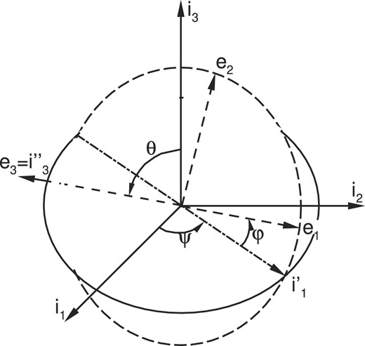
Euler’s angles.
The motion of the centre of mass of a dust grain is given by
where |$\boldsymbol{r}$| and |$\boldsymbol{v}_d$| are the radius vector and the velocity of the centre of mass in the fixed cometocentic frame, md is the grain’s mass, and |$\boldsymbol{R}$| is a resultant vector of external forces, that is, the sum of the gravity |$\boldsymbol{F}_N$| and the aerodynamic force |$\boldsymbol{F}_a$|.
From the law of variation of the angular momentum, we can get in the moving frame the Euler dynamic equations
and the Euler kinematic equation
where |$\boldsymbol{M} =\boldsymbol{M}_N + \boldsymbol{M}_a$| is a resultant torque of external forces, that is, the sum of the gravitational |$\boldsymbol{M}_N$| and aerodynamic |$\boldsymbol{M}_a$| torques, |$\boldsymbol{\omega }$| is a vector of instantaneous angular velocity, |$\boldsymbol{I}$| is a tensor of inertia, and |$\boldsymbol{i}_3$|, |$\boldsymbol{i}^{\prime }_1$|, |$\boldsymbol{e}_3$| are the unit vectors (see Fig. 1).
The equations (1), (2), and (3) form a close system of differential equations that describes motion of a grain.
The gravitational and aerodynamic force |$\vec{F}_N$| and |$\vec{F}_a$| are given by
and the gravitational and aerodynamic torque |$\boldsymbol{M}_N$| and |$\boldsymbol{M}_a$| are given by
where p, τ are the gas pressure and the shear stress of the elementary surface element with area dS, |$\boldsymbol{n}$| is the unit vector of outward normal to the element, |$\boldsymbol{v}_r$| is the gas–grain relative velocity, ϱd is the specific density of the dust grain, dΓ is the elementary volume of the grain, Vd is the volume of the grain, and |$\boldsymbol{l}$| is the radius vector from grain’s centre of mass to dΓ or dS. In case of a cometary atmosphere, the mean-free path of the molecules λ is much larger than the grain size ad (i.e. λ ≫ ad). Therefore, the pressure p and the shear stress τ can be computed as in a free molecular flow:
Here it is assume that molecules are reflected diffusely, |$p_g=\rho v_r^{\prime 2}/(2s^{\prime 2})$|, |$s^{\prime }= v_r^{\prime } \sqrt{m_g/(2 k_B T_g)}$| is gas–dust speed ratio, |$\boldsymbol{v}_r^{\prime }= \boldsymbol{v}_g - \boldsymbol{v}_d^{\prime }$| being the gas–dust relative velocity (|$v_d^{\prime }$| is the velocity of the surface element accounting rotation of the grain), β is an angle between |$\boldsymbol{v}_r^{\prime }$| and inward normal of the element. The pressure p is co-directional to the inward normal of the element, the shear stress τ is co-directional with the projection of |$\boldsymbol{v}_r^{\prime }$| on the element’s plane.
For given shapes of grains the integrals in equations (5) and (7) can be pre-computed for different orientations of the grain with respect to the flow and various values of Tg/Tg and s′. Then the approximate expressions for the aerodynamic force and torque are
where CD and |$\boldsymbol{C}_M$| are the averaged coefficients of aerodynamic drag and torque, ad and σd are the characteristic size and cross-section of the particle.
This paper neglects the solar pressure and the solar tidal forces that affect significantly the dust motion out of the acceleration zone over long times (weeks and longer). In addition, for particles equal and larger than mm-sized these effects are important also just outside the dust acceleration zone. The rigorous computation in the heliocentric reference frame of the dust motion out of cometary Hill’s sphere can be found in Fulle et al. (1995).
Following Zakharov et al. (2018) and Zakharov et al. (2021) we introduce the following dimensionless variables: |$\tilde{v}_g = v_g/v_g^{max}$|, |$\tilde{v}_d = v_d/v_g^{max}$|, |$\tilde{r} = r/R_N$|, |$\tilde{t} = t/\Delta t$|, |$\tilde{\rho }_g=\rho _g / \rho _s$|. Here |$v_g^{max}=\sqrt{\gamma \frac{\gamma +1}{\gamma -1} \frac{k_b}{m_g} T_s}$| is the theoretical maximum velocity of gas expansion, ρs and Ts are the gas density and temperature on the sonic surface (i.e. where the gas velocity is equal the local sound velocity |$v_\ast =\sqrt{\gamma k_B T_g/m_g}$|) at the subsolar point, γ is the specific heat ratio, RN is the characteristic linear scale (e.g. the radius of the nucleus), and |$\Delta t=R_N/v_g^{max}$|. In addition, we introduce |$\tilde{\boldsymbol{g}}$| via normalizing |$\boldsymbol{g}$| on |$G m_N/R_N^2$| (therefore, in the case of a spherical nucleus |$\tilde{\boldsymbol{g}} =-\tilde{\boldsymbol{r}}/|{\tilde{r}}^3|$|), |$\tilde{I}=I/(m_d a^2_d)$| and |$\tilde{\omega }=\omega /(v_g^{max}/a_d)$|.
Using the dimensionless variables, the equations of translational motion of dust grain can be rewritten in dimensionless form
The equation of the rotational motion in the dimensionless form is
These equations contain three dimensionless parameters Iv, Fu, and RN/ad. The parameter Iv characterizes the efficiency of entrainment of the particle within the gas flow (i.e. the ability of a dust particle to adjust to the gas velocity)
Here, Qg is the total gas production rate [s−1] of a spherical nucleus of radius RN with uniform gas production over the surface equal to the gas production at subsolar point. The parameter Fu characterizes the efficiency of gravitational attraction
The dimensionless parameters |$\rm Iv$|, |$\rm Fu$| for the first time were introduced in Zakharov et al. (2018). In order to define |$\rm Iv, Fu$| it is necessary to know: mg, γ, ρs, Ts, RN, mN, σd, and md (or ad and ϱd).
3 RESULTS
In a given gas flow field, if two dust grains have same Iv and Fu their translational motion is similar. If, in addition, they have same RN/ad then their rotational motion is similar as well. We remind that the influence of solar pressure is assumed negligible.
In the following section, we derive scaling laws for the terminal dust velocity |$\tilde{v}^t_d$| and rotational frequency |$\tilde{\omega }^t$|, that is, the velocity and rotational frequency that a dust grain has after decoupling with the gas flow. As was derived from observational, the dust acceleration limited within six nuclear radii for a broad range of particle sizes (Gerig et al. 2018). The numerical studies (e.g. Zakharov et al. 2018; Ivanovski 2017) also show that gas and dust decoupling occurs within first ten radii of the nucleus.
At distances r/RN > 10 the time derivatives |$\frac{d \tilde{\boldsymbol{\omega }}}{d \tilde{t}} \rightarrow$|0 and |$\frac{d \tilde{\boldsymbol{v}}_d}{d\tilde{t}} \rightarrow$|0, the gas velocity is close to |$v_g^{max}$| therefore |$\tilde{v}_g \approx$|1. As was shown in Zakharov et al. (2021) for the range of conditions Iv < 0.1 and Fu < 0.01 · Iv, the ratio of terminal velocities of two dust particles (labelled 0 and 1) in a given gas flow field is
Therefore, the scaling law for the dust particle terminal velocity is
where |$\tilde{v}^t_{di}=v^t_{di}/v^{max}_g$|.
The scaling law for the dust particle rotational frequency follows from the equation (14) under assumption of negligible influence of gravitational torque (Iv ≫ Fu)
where |$\tilde{\omega }^t_{di} = \omega ^t_{di} a_{d i}/v^{max}_g$|. The value of |$\tilde{v}^t_d$| is taken from equation (18) or, if |$\tilde{v}^t_d \ll 1$|, the equation (20) becomes
In order to verify these scaling relations we use the numerically computed data from Ivanovski (2017) and Moreno et al. (2022). Ellipsoids of revolution with different aspect ratios were considered in Ivanovski (2017) (see Fig. 2). Irregularly shaped particles were considered in Moreno et al. (2022) (see Fig. 3). The gas coma was approximated by a spherically symmetric expanding gas (pure H2O) flow. It was assumed that the nucleus has radius RN = 2 [km], mass mN = 1013 [kg] and the surface temperature Ts = 200 [K].
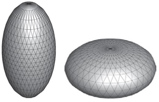
Model particles used in the dynamical calculations in Ivanovski (2017). Prolate (right) and oblate (left).
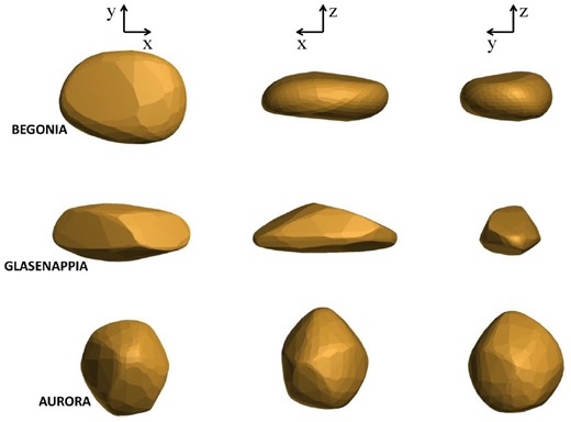
Model particles used in the dynamical calculations in Moreno et al. (2022). On the top row of panels, BEGONIA shape model particle, having a flattened shape, on the middle row GLASENAPPIA shape model particle (elongated), and on the bottom row, AURORA shape model particle displaying a rounded shape. Approximate outer dimensions of the particles relative are (1.00 × 0.72 × 0.36), (1.00 × 0.43 × 0.36), and (1.00 × 1.09 × 1.14), respectively.
At first, we test the scaling on the results of numerical simulations given in Ivanovski (2017). As the referential case for the scaling we use numerical solution for ad = 10−4 [m], Qg = 1026 [s−1], ϱd = 100 [kg m–3], which gives |$v_d^t$| = 4.2 [m s–1] and ωt = 0.09 [s−1] for the prolate spheroid (case a03g1d1pr), and |$v_d^t$| = 5.0 [m s–1] and ωt = 0.1 [s−1] for the oblate spheroid (case a03g1d1ob). This case corresponds to Iv = 1.280 · 10−5 and Fu = 3.860 · 10−7 (i.e. Iv/Fu = 33.16). Tables 1 and 2 show the comparison of scaled (via eqs. (17) and (20)) and numerically computed values from Ivanovski (2017) for different values of ad, Qg, and ϱd. Using the two groups of results in Tables 1 and 2, we summarize the corresponding scaling precision in Fig. 4, left and 4, right, respectively. We note that in the cases of prolate spheroids (Table 1 and Fig. 4, right) high-gas production rate and small particles lead to better precision in scaling for the velocity than for the rotation. Nevertheless, the rotation precision is within maximum 40 per cent. In the cases of oblate spheroid (Table 2 and Fig. 4, right) an increase in the gas production rate produces better precision in scaling for the velocity than for the rotation. All this trend is expected since higher gas production rate is more efficient for particles with large cross-sections than the ones of smaller sizes, provided equal particle masses for all considered particles. Furthermore, in case of large particles we have an opposite trend, less precision in velocity scaling, and better one for rotation. Only 2 cases of 38 considered show precision worse than 35 per cent and one worse than 100 per cent for the rotation. However, for the remaining cases, we note that the scaling achieves precision of more than 60–70 per cent for both prolate and oblate spheroids and more than 95 per cent for the velocity of prolate spheroids.

Comparison of scaled (via eqs. (17) and (20) with numerically computed values from Ivanovski (2017). The referential case is a03g1d1pr (prolate spheroid) with ad = 10−4 [m], Qg = 1026 [s−1], ρd = 100 [kg m–3], |$v_d^t$| = 4.2 [m s–1], ωt = 0.09 [s−1]. The case’s labels correspond to the Tables B.4–B.6 in Ivanovski (2017).
| Case | ad | Qg | ρd | Iv | Iv/Fu | |$v_d^t$|[m s–1] | ωt[s−1] | εv | εω | ||
|---|---|---|---|---|---|---|---|---|---|---|---|
| [m] | [s−1] | [kg m–3] | Scaled | Computed | Scaled | Computed | per cent | per cent | |||
| a03g1d2pr | 10−4 | 1026 | 1000.0 | 1.28· 10−6 | 3.315 | 1.328 | 1.0 | 0.0285 | 0.02 | 32.80 | 42.50 |
| a03g2d1pr | 10−4 | 1027 | 100.0 | 1.28· 10−4 | 3.315· 102 | 13.282 | 13.7 | 0.2818 | 0.23 | 3.05 | 22.52 |
| a03g2d2pr | 10−4 | 1027 | 1000.0 | 1.28· 10−5 | 3.315· 101 | 4.200 | 4.2 | 0.0900 | 0.09 | 0.0 | 0.0 |
| a03g3d1pr | 10−4 | 1028 | 100.0 | 1.28· 10−3 | 3.315· 103 | 42.000 | 43.0 | 0.8632 | 0.7 | 2.33 | 23.31 |
| a03g3d2pr | 10−4 | 1028 | 1000.0 | 1.28· 10−4 | 3.315· 102 | 13.282 | 13.7 | 0.2818 | 0.23 | 3.05 | 22.52 |
| a03g4d1pr | 10−4 | 1029 | 100.0 | 1.28· 10−2 | 3.315· 104 | 132.816 | 127.5 | 2.4504 | 2.0 | 4.17 | 22.52 |
| a03g4d2pr | 10−4 | 1029 | 1000.0 | 1.28· 10−3 | 3.315· 103 | 42.000 | 43.0 | 0.8632 | 0.7 | 2.33 | 23.31 |
| b03g1d1pr | 10−3 | 1026 | 100.0 | 1.28· 10−6 | 3.315 | 1.328 | 1.0 | 0.0090 | 0.01 | 32.80 | 10.00 |
| b03g2d1pr | 10−3 | 1027 | 100.0 | 1.28· 10−5 | 3.315· 101 | 4.200 | 4.2 | 0.0285 | 0.025 | 0.0 | 14.00 |
| b03g2d2pr | 10−3 | 1027 | 1000.0 | 1.28· 10−6 | 3.315 | 1.328 | 1.0 | 0.0090 | 0.008 | 32.80 | 12.50 |
| b03g3d1pr | 10−3 | 1028 | 100.0 | 1.28· 10−4 | 3.315· 102 | 13.282 | 13.5 | 0.0891 | 0.08 | 1.62 | 11.37 |
| b03g3d2pr | 10−3 | 1028 | 1000.0 | 1.28· 10−5 | 3.315· 101 | 4.200 | 4.2 | 0.0285 | 0.025 | 0.0 | 14.00 |
| b03g4d1pr | 10−3 | 1029 | 100.0 | 1.28· 10−3 | 3.315· 103 | 42.000 | 43.0 | 0.2730 | 0.2 | 2.33 | 36.50 |
| b03g4d2pr | 10−3 | 1029 | 1000.0 | 1.28· 10−4 | 3.315· 102 | 13.282 | 14.0 | 0.0891 | 0.08 | 5.13 | 11.37 |
| c03g2d1pr | 10−2 | 1027 | 100.0 | 1.28· 10−6 | 3.315 | 1.328 | 1.0 | 0.0029 | 0.002 | 32.80 | 45.00 |
| c03g3d1pr | 10−2 | 1028 | 100.0 | 1.28· 10−5 | 3.315· 101 | 4.200 | 4.2 | 0.0090 | 0.008 | 0.0 | 12.50 |
| c03g3d2pr | 10−2 | 1028 | 1000.0 | 1.28· 10−6 | 3.315 | 1.328 | 1.0 | 0.0029 | 0.003 | 32.80 | 3.33 |
| c03g4d1pr | 10−2 | 1029 | 100.0 | 1.28· 10−4 | 3.315· 102 | 13.282 | 13.7 | 0.0282 | 0.03 | 3.05 | 6.00 |
| c03g4d2pr | 10−2 | 1029 | 1000.0 | 1.28· 10−5 | 3.315· 101 | 4.200 | 4.2 | 0.0090 | 0.008 | 0.0 | 12.50 |
Comparison of scaled (via eqs. (17) and (20)) with numerically computed values from Ivanovski (2017). The referential case is a03g1d1ob (obolate spheroid) with ad = 10−4 [m], Qg = 1026 [s−1], ρd = 100 [kg m–3], |$v_d^t$| = 5.0 [m s–1], ωt = 0.1 [s−1]. The case’s labels correspond to the Tables B.8–B.10 in Ivanovski (2017).
| Case | ad | Qg | ρd | Iv | Iv/Fu | |$v_d^t$|[m s–1] | ωt[s−1] | εv | εω | ||
|---|---|---|---|---|---|---|---|---|---|---|---|
| [m] | [s−1] | [kg m–3] | Scaled | Computed | Scaled | Computed | per cent | per cent | |||
| a03g1d2ob | 10−4 | 1026 | 1000.0 | 1.28· 10−6 | 3.315 | 1.581 | 1.3 | 0.0317 | 0.03 | 21.6 | 5.80 |
| a03g2d1ob | 10−4 | 1027 | 100.0 | 1.28· 10−4 | 3.315· 102 | 15.811 | 14.0 | 0.3125 | 0.30 | 12.9 | 4.18 |
| a03g2d2ob | 10−4 | 1027 | 1000.0 | 1.28· 10−5 | 3.315· 101 | 5.000 | 5.0 | 0.1000 | 0.10 | 0.00 | 0.00 |
| a03g3d1ob | 10−4 | 1028 | 100.0 | 1.28· 10−3 | 3.315· 103 | 50.000 | 48.0 | 0.9513 | 1.00 | 4.17 | 4.87 |
| a03g3d2ob | 10−4 | 1028 | 1000.0 | 1.28· 10−4 | 3.315· 102 | 15.811 | 15.0 | 0.3125 | 0.10 | 5.41 | 213.0 |
| a03g4d1ob | 10−4 | 1029 | 100.0 | 1.28· 10−2 | 3.315· 104 | 158.114 | 140.0 | 2.6385 | 2.20 | 12.9 | 19.9 |
| a03g4d2ob | 10−4 | 1029 | 1000.0 | 1.28· 10−3 | 3.315· 103 | 50.000 | 48.0 | 0.9513 | 1.00 | 4.17 | 4.87 |
| b03g1d1ob | 10−3 | 1026 | 100.0 | 1.28· 10−6 | 3.315 | 1.581 | 1.3 | 0.0100 | 0.01 | 21.6 | 0.370 |
| b03g2d1ob | 10−3 | 1027 | 100.0 | 1.28· 10−5 | 3.315· 101 | 5.000 | 4.8 | 0.0316 | 0.03 | 4.17 | 5.41 |
| b03g2d2ob | 10−3 | 1027 | 1000.0 | 1.28· 10−6 | 3.315 | 1.581 | 1.3 | 0.0100 | 0.01 | 21.6 | 0.370 |
| b03g3d1ob | 10−3 | 1028 | 100.0 | 1.28· 10−4 | 3.315· 102 | 15.811 | 15.0 | 0.0988 | 0.10 | 5.41 | 1.17 |
| b03g3d2ob | 10−3 | 1028 | 1000.0 | 1.28· 10−5 | 3.315· 101 | 5.000 | 4.8 | 0.0316 | 0.03 | 4.17 | 5.41 |
| b03g4d1ob | 10−3 | 1029 | 100.0 | 1.28· 10−3 | 3.315· 103 | 50.000 | 48.0 | 0.3008 | 0.30 | 4.17 | 0.278 |
| b03g4d2ob | 10−3 | 1029 | 1000.0 | 1.28· 10−4 | 3.315· 102 | 15.811 | 15.0 | 0.0988 | 0.10 | 5.41 | 1.17 |
| c03g2d1ob | 10−2 | 1027 | 100.0 | 1.28· 10−6 | 3.315 | 1.581 | 1.2 | 0.0032 | 0.003 | 31.8 | 5.80 |
| c03g3d1ob | 10−2 | 1028 | 100.0 | 1.28· 10−5 | 3.315· 101 | 5.000 | 4.6 | 0.0100 | 0.010 | 8.70 | 0.00 |
| c03g3d2ob | 10−2 | 1028 | 1000.0 | 1.28· 10−6 | 3.315 | 1.581 | 1.2 | 0.0032 | 0.003 | 31.8 | 5.80 |
| c03g4d1ob | 10−2 | 1029 | 100.0 | 1.28· 10−4 | 3.315· 102 | 15.811 | 15.5 | 0.0313 | 0.030 | 2.01 | 4.18 |
| c03g4d2ob | 10−2 | 1029 | 1000.0 | 1.28· 10−5 | 3.315· 101 | 5.000 | 5.0 | 0.0100 | 0.008 | 0.00 | 25.0 |
The precision of the scaling is estimated by the difference of numerically computed and scaled values with respect to numerically computed value
For both prolate and oblate grains the scaled values of |$v_d^t$| and ωt are in good agreement with numerically computed ones if Iv/Fu > 10. The large difference in scaled and numerically computed frequency in case a03g3d2ob is probably due to inaccuracy of numerical solution.
And further, we test the scaling on the results of numerical simulations given in Moreno et al. (2022). As the referential case for the scaling we use numerical solution for ad = 10−3 [m], Qg = 3 · 1028 [s−1], ϱd = 800 [kg m–3], which gives |$v_d^t$| = 10.0 [m s–1] and ωt = 1.6 [s−1] for the Begonia shape, and |$v_d^t$| = 10.0 [m s–1] and ωt = 2.7 [s−1] for the Glasenappia shape, and |$v_d^t$| = 9.34 [m s–1] and ωt = 0.9 [s−1] for the Aurora shape. This case corresponds to Iv = 4.799 · 10−5 and Fu = 3.860 · 10−7 (i.e. Iv/Fu = 124.3). Table 3 shows the comparison of scaled (via eqs. (17) and (20)) and numerically computed values from Moreno et al. (2022) for different values of ad and Qg.
Comparison of scaled (via eqs. (17) and (20)) with numerically computed values from Moreno et al. (2022). The referential case is ad = 10−3 [m], Qg = 3 · 1028 [s−1], ϱd = 800 [kg m–3] which gives for |$v_d^t$| [m s–1] and ωt [s−1] the following values: 10.0 and 1.6 for Begonia; 10.0 and 2.7 for Glasenappia; 9.34 and 0.9 for Aurora.
| Case | ad | Qg | Iv | Iv/Fu | |$v_d^t$|[m s–1] | ωt[s−1] | εv | εω | ||
|---|---|---|---|---|---|---|---|---|---|---|
| [m] | [s−1] | Scaled | Computed | Scaled | Computed | per cent | per cent | |||
| Begonia | 10−3 | 1· 1027 | 1.6· 10−6 | 4.144 | 1.83 | 1.6 | 0.29 | 0.3 | 14.37 | 3.33 |
| Glasenappia | 10−3 | 1· 1027 | 1.6· 10−6 | 4.144 | 1.83 | 1.6 | 0.50 | 0.5 | 14.37 | 0.0 |
| Aurora | 10−3 | 1· 1027 | 1.6· 10−6 | 4.144 | 1.71 | 1.45 | 0.17 | 0.15 | 17.93 | 13.33 |
| Begonia | 10−2 | 3· 1028 | 4.8· 10−6 | 12.43 | 3.16 | 3.06 | 0.16 | 0.09 | 3.27 | 77.78 |
| Glasenappia | 10−2 | 3· 1028 | 4.8· 10−6 | 12.43 | 3.16 | 3.10 | 0.27 | 0.20 | 1.94 | 35.00 |
| Aurora | 10−2 | 3· 1028 | 4.8· 10−6 | 12.43 | 2.95 | 2.85 | 0.09 | 0.04 | 3.51 | 125.00 |
| Begonia | 10−4 | 3· 1028 | 4.8· 10−4 | 1.243· 103 | 31.62 | 31.50 | 15.62 | 97.5 | 0.38 | 83.98 |
| Glasenappia | 10−5 | 3· 1028 | 4.8· 10−3 | 1.243· 104 | 100.00 | 98.20 | 243.57 | 780.00 | 1.83 | 68.77 |
| Begonia | 10−6 | 3· 1028 | 4.8· 10−2 | 1.243· 105 | 316.23 | – | 1067.13 | – | – | – |
| Glasenappia | 10−6 | 3· 1028 | 4.8· 10−2 | 1.243· 105 | 316.23 | – | 1800.78 | – | – | – |
| Aurora | 10−6 | 3· 1028 | 4.8· 10−2 | 1.243· 105 | 295.36 | – | 620.24 | – | – | – |
Table 3 shows that precision of scaling of |$v_d^t$| increases with increase of Iv/Fu.
In order to estimate the precision of the scaling with respect to the shape irregularity we have calculated the dispersion of the moments of inertia of the considered shapes. The dispersion was calculated as a standard deviation of the three moments of inertia of a given shape divided on their mean value. The purpose of this estimation is that the dispersion calculated in this way is dimensionless and can be easily used for comparison in all available cases. The general trend is: the higher the dispersion is, the better the scaling is. The only deviation from this observation is the case of a prolate spheroid and this can be owing to the fact that in the cases of Tables 1 and 2 the rotational motion is happening only in one plane as discussed in Ivanovski (2017). In cases of Moreno et al. (2022), the dispersion for the three shapes is the following: 31 per cent for Begonia, 47 per cent for Glasenappia and 5 per cent for Aurora. As can be checked in Table 3 the scaling works better for more irregular shapes like Glasenappia and Begonia ones. The shapes with a smaller dispersion can easily and often change their axis of rotation that results in more complex rotational motion, that is, seems more difficult to be precisely obtained by scaling.
In addition, Table 3 shows scaled |$v_d^t$| and ωt for micron size grains for which the numerical solution is not given in Moreno et al. (2022) due to excessive computational demands. It should be noted that too fast-rotating grains may violate the condition (10) from Ivanovski (2017) (it constrains applicability of free molecular approximation for evaluation of pressure p and shear stress τ).
4 CONCLUSIONS
In the present paper, we focus on derivation of scaling laws of rotational motion applicable for any shape of particles. We use a set of universal, dimensionless parameters characterizing the dust motion in the inner cometary coma. Based on the dimensionless description of the translational and rotational motion of dust particles we derived scaling relations for the terminal velocity and rotational frequency of non-spherical grains. The comparison of scaled values with available numerically computed data shows that the proposed scaling relations provide estimations of |$v_d^t$| and ωt with sufficient precision. Therefore, having one numerically computed ‘reference case’ one can get order of magnitude estimation for other cases via simple scaling. This allows avoiding long-time and huge electric power consumption numerical simulations.
ACKNOWLEDGEMENTS
This research was supported by the Italian Space Agency (ASI) within the ASI-INAF agreements I/032/05/0, I/024/12/0, 2020-4-HH.0, and N. 2023-14-HH.0. The work of NYB is funded by the Ministry of Science and Higher Education of the Russian Federation as part of the World-class Research Centre programme: Advanced Digital Technologies (contract no. 075-15-2022-311 dated 2022 April 20). This work was supported by the International Space Science Institute (ISSI) through the ISSI International Team ‘Characterization of cometary activity of 67P/Churyumov–Gerasimenko comet’.
DATA AVAILABILITY
This work uses simulated data, generated as described diligently in the text. If you want to present additional material which would interrupt the flow of the main paper, it can be placed in an Appendix which appears after the list of references.
