


ABSTRACT
We search for high-velocity stars in the inner region of the Galactic bulge using a selected sample of red clump stars. Some of those stars might be considered hypervelocity stars (HVSs). Even though the HVSs ejection relies on an interaction with the supermassive black hole (SMBH) at the centre of the Galaxy, there are no confirmed detections of HVSs in the inner region of our Galaxy. With the detection of HVSs, ejection mechanism models can be constrained by exploring the stellar dynamics in the Galactic centre through a recent stellar interaction with the SMBH. Based on a previously developed methodology by our group, we searched with a sample of preliminary data from version 2 of the Vista Variables in the Via Lactea (VVV) Infrared Astrometric Catalogue (VIRAC2) and Gaia DR3 data, including accurate optical and near-infrared proper motions. This search resulted in a sample of 46 stars with transverse velocities larger than the local escape velocity within the Galactic bulge, of which four are prime candidate HVSs with high-proper motions consistent with being ejections from the Galactic centre. Adding to that, we studied a sample of reddened stars without a Gaia DR3 counterpart and found 481 stars with transverse velocities larger than the local escape velocity, from which 65 stars have proper motions pointing out of the Galactic centre and are candidate HVSs. In total, we found 69 candidate HVSs pointing away from the Galactic centre with transverse velocities larger than the local escape velocity.
1 INTRODUCTION
The Galactic bulge is the region 2.5 kpc around the Galactic centre (GC), and within the Λ cold dark matter paradigm, it was the first Galactic structure that formed through the hierarchical merging of less-massive structures (Steinmetz & Muller 1995; Springel & Hernquist 2005; Barbuy, Chiappini & Gerhard 2018). The environment in such region is extreme, with high stellar crowding and in its centre resides a supermassive black hole (SMBH), Sagittarius A* (Sgr A*), with a mass of |$4.3\times 10^6\, \mathrm{{\rm M}_{\odot }}$| (Rodriguez 1978; Ghez et al. 2008; Genzel, Eisenhauer & Gillessen 2010; GRAVITY Collaboration 2022). The high stellar density favours interactions amongst stars and between stars and Sgr A*.
An interaction between a triple system can result in one of the stars acquiring a velocity larger than the local standard of rest. The identification of a star after the interaction gives insight into the dynamics surrounding the interaction itself. For example Blaauw (1961) showed that runaway stars with peculiar velocities larger than 30 |$\mathrm{km\, s^{-1}}$| can form after a binary stellar system disruption in the supernova explosion of one of its components. Poveda, Ruiz & Allen (1967) investigated dynamical stellar interactions during the collapse of small clusters of massive stars, noting that runaway stars can result from such interactions acquiring velocities that exceed 35 |$\mathrm{km\, s^{-1}}$| and in some cases reaching nearly 200 |$\mathrm{km\, s^{-1}}$|.
Hypervelocity stars (HVSs) are the fastest stars in the Galaxy. They were initially defined as stars ejected after a three-body interaction of a binary system with Sgr A*; one star is ejected as an HVS, while the other remains attached to the SMBH as an S-Star1 (Hills 1988). This is known as the Hills mechanism, the most accepted and successful HVS ejection scenario, but not the only one. Alternative mechanisms that explain how an HVS acquires its large velocity include the interaction between a binary massive black hole (bMBH) and a single star (Yu & Tremaine 2003); or between a globular cluster and an SMBH (Brown 2015; Capuzzo-Dolcetta & Fragione 2015; Fragione, Capuzzo-Dolcetta & Kroupa 2017; Irrgang et al. 2019; Neunteufel 2020). In a tidal disruption event, the ejection velocity of a binary component is proportional to the binary components separation and the mass of the BH: vej ∝ (a)−1/2(M/M⊙)1/6. Given the mass of Sgr A*, |$4\times 10^6\, \mathrm{{\rm M}_{\odot }}$|, HVSs can be ejected at up to |$\sim 4000$||$\mathrm{km\, s^{-1}}$| (Hills 1988; Sari, Kobayashi & Rossi 2010; Rossi et al. 2017, 2021), which is larger than the escape velocity. The local escape velocity is ∼830 |$\mathrm{km\, s^{-1}}$| in the GC, ∼320 |$\mathrm{km\, s^{-1}}$| in the halo (50 kpc), and ∼530 |$\mathrm{km\, s^{-1}}$| at the Sun location (Rossi et al. 2017; Deason et al. 2019). Besides explaining the extreme velocities of HVSs, the Hills mechanism can explain the presence of young stars close to the GC, where an in situ formation is unlikely because a molecular cloud would not survive such an extreme environment. In this scenario, the young stars close to the GC could be the remnants of a binary system disruption by Sgr A* (Hills 1988; Generozov 2021).
Since the first discovery by Brown et al. (2005), there are around 20 confirmed HVSs and over 500 candidates (Boubert et al. 2018). The high stellar crowding as well as large and patchy extinction in the central regions of the Milky Way hampered the detection of HVSs close to their origin. They were identified in a more favourable environment, the Milky Way halo, with velocities ranging from 300 up to 1700 |$\mathrm{km\, s^{-1}}$|, exceeding the local escape speed (e.g. Kollmeier et al. 2009; Kenyon et al. 2014; Palladino et al. 2014; Brown et al. 2018). Almost all of them are B-type stars with masses between 2.5 and 4 M⊙, except for the fastest star amongst them: HVS-S5 (Koposov et al. 2020), an A-type star with a velocity of 1700 |$\mathrm{km\, s^{-1}}$|. This star is also the only HVS whose travel direction and orbit points to the origin from the GC, favouring the Hills mechanism as responsible for its ejection. For other cases, the Hills mechanism can be ruled out, as the orbits of the stars suggest an origin in the disc, in the Magellanic Clouds (e.g. Przybilla et al. 2008; Lennon et al. 2017; Boubert, Erkal & Gualandris 2020; Evans et al. 2021), or the Sagittarius dwarf spheroidal galaxy (Huang et al. 2021; Li et al. 2022).
In a recent study, Li et al. (2023) combined multiple spectroscopic large surveys and found that the ejection from dwarf galaxies and globular clusters is more prominent for the metal-poor late-type halo HVS production. Based on Gaia data, and follow-up spectroscopic observations, El-Badry et al. (2023) identified four hypervelocity white dwarf (WD) stars, travelling at space velocities larger than 1300 |$\mathrm{km\, s^{-1}}$| after the double detonation – helium in the surface, followed by carbon in the core – of the more massive WD in a binary system of WDs. The objects have crossed the Galactic plane on multiple occasions, getting accelerated or slowed down, but none of them have trajectories that trace back to the GC. The analysis of positions and velocity distributions of the fastest stars in proximity to the GC offers insights into the shape of the Galactic potential (Kenyon et al. 2008).
HVSs within the Galactic bulge provide additional constraints on the characteristics of the stellar population in that particular region of the Galaxy. This includes the joint constraints of the stellar initial mass function of the GC and the HVS ejection rate, and the binary separation distribution (see Rossi, Kobayashi & Sari 2014; Rossi et al. 2017; Marchetti, Evans & Rossi 2022; Evans, Marchetti & Rossi 2022b).
Luna, Minniti & Alonso-García (2019) presented the first HVS candidates in the Galactic bulge using the Vista Variables in the Via Lactea (VVV) near-infrared (NIR) survey data. This work is extended here using the Gaia DR3 data in combination with a larger set of improved VVV-based NIR proper motions: VVV Infrared Astrometric Catalogue 2 (VIRAC2). We search for HVS candidates that can be further studied spectroscopically to confirm their nature and constrain their origin.
The paper is organized as follows: in Section 2, we describe the data sets. In Section 3, we present the selection of red clump stars and the computation of distances and tangential velocities. The resulting sample of high-velocity stars and HVSs candidates from the VIRAC2-Gaia DR3 crossmatch is presented in Section 4 and in Section 5 the equivalent sample of those stars having only VIRAC2 data. In Section 6, we summarize our conclusions.
2 THE Gaia DR3 AND VIRAC2 CATALOGUES
2.1 Gaia DR3
The Gaia DR3 provides, amongst other information, optical photometry (G, GBP, and GRP) and astrometry (parallaxes and proper motions) for ∼1.5 billion sources in the Galaxy, with 34 months of observations (Gaia Collaboration 2022). Gaia DR3 doubled the precision in proper motions and improved by 30 per cent the precision in parallaxes with respect to Gaia DR2. In the same vein, the errors improved by a factor of ∼2.5 in proper motions and up to 40 per cent in parallaxes (Lindegren et al. 2016; van Leeuwen et al. 2017; Gaia Collaboration 2021; Fabricius et al. 2021).
The survey has completeness below 60 per cent for sources at G ∼ 19 or fainter and in stellar densities of about |$5\times 10^5\, \mathrm{stars}\, \deg ^{-2}$|, which is characteristic of crowded fields such as globular clusters. Its completeness further drops below 20 per cent even for brighter sources in fields with stellar densities of about |$10^6-10^7\, \mathrm{stars}\, \deg ^{-2}$| that are found in the Galactic bulge (Fabricius et al. 2021; Cantat-Gaudin et al. 2023). In the present study, we select Gaia DR3 sources that are matched with the VIRAC2 data (see next section) in coordinates.
2.2 VIRAC2
The VVV survey (Minniti et al. 2010) and its extension, the VVV eXtended survey (VVVX), acquired multi-epoch observations between 2010 and 2023 (hereafter we always refer to the survey as VVV, but it includes also the VVVX data). VVV produced a map of the Galactic bulge and southern part of the disc (|$-130\deg \lt \, l\lt\, 20\deg$| and |$-15\deg \lt \, b\lt \, 10\deg$|) covering |$\sim 1700\deg ^2$| in three NIR passbands: J(1.25 μm), H(1.64 μm), and Ks(2.14 μm) [the VVV original footprint is also covered in Z(0.87 μm) and Y(1.02 μm) bands]. For further information about the VVV survey and its data quality, we refer to publications by Minniti et al. (2010), Saito et al. (2012), Alonso-García et al. (2018), and Surot et al. (2019b). VIRAC2 (Smith et al., in preparation) is the second data release of the VIRAC (Smith et al. 2018). VIRAC2 is constructed from the PSF photometry catalogue, while VIRAC data are derived from aperture photometry. VIRAC2 is 90 per cent complete up to Ks ∼ 16 across the VVV bulge area (Sanders et al. 2022). Its proper motions are anchored to Gaia DR3 absolute reference frame. Luna et al. (2023) tested the reliability of VIRAC2 proper motions and their errors.
In our study, we use preliminary VIRAC2 data, and adopted the following quality selection criteria: (i) sources with a complete (5-parameter) astrometric solution, (ii) non-duplicates, (iii) sources that are detected in at least 20 per cent of the observations,2 and (iv) sources with unit weight error (uwe) uwe < 1.2. The latter is used as a threshold to select single sources with good astrometric measurements.
3 SELECTION OF RED CLUMP SOURCES
Red clump (RC) stars are in the helium core-burning phase on their second ascent towards the giant branch (see Girardi 2016, for a review). They are easily identified in nearby stellar systems because they occupy a well-defined region in colour–magnitude diagrams (CMDs). They have a characteristic luminosity and exhibit minimal variability, which makes them a useful standard candle for distance determination (Alves et al. 2002; Ruiz-Dern et al. 2018).
Using the VIRAC2 data set, we select a region in the inner part of the Galactic bulge, in a box within |$-5\deg \lt \, l\lt \, 5\deg$| and |$-3\deg \lt \, b\lt \, 3\deg$|. The total number of sources from VIRAC2 within the 60 deg2 region is |$112\, 599\, 161$|. In the same area, there are |$36\, 101\, 569$| sources in Gaia.
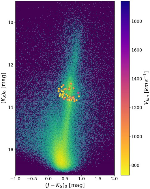
In Fig. 1, we show the J − Ks versus Ks CMD for all the stars in the 60 deg2 bulge area centred on the GC. The blue sequence at J − Ks ≤ 0.6 mag, populated by the main-sequence disc, and the redder red giant branch (RGB) bulge sequence merge at Ks > 15 mag. The RGB is the nearly vertical sequence ranging in colour around J − Ks ∼ 0.8 − 1.1. Due to very high reddening in the centre-most regions of the bulge the RGB fans along the reddening vector covering the entire J − Ks range of the CMD. There are three overdensities along the RGB in the J − Ks CMD (Fig. 1). While the most obvious one, which we highlight inside an orange box in Fig. 1, corresponds to the RC stars from the bulge, the nature of the other two overdensities is more uncertain (Nataf et al. 2011, 2013; Alonso-García et al. 2018; Gonzalez et al. 2018).
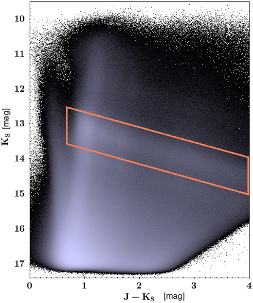
VVV NIR CMD of the 60 deg2 studied region towards the Galactic bulge. The box encloses the area used for the RC sources selection.
In the CMD, we select the overdensity traced by the RC stars inside the orange box marked with a solid line in Fig. 1. These stars are selected within ±0.5 mag along the reddening vector
We have used the Ks total-to-selective ratio from (Alonso-García et al. 2017)
where the infrared colour excess of the RC stars is E(J − Ks) = (J − Ks) − (J − Ks)0 and each star has an individual value taken from the reddening map of Sanders et al. (2022).
The orange box is centred on the RC. The intrinsic colour of the Galactic bulge RC is (J − Ks)0 = 0.68 mag (Alves et al. 2002; Gonzalez et al. 2012; Ruiz-Dern et al. 2018), but the bulk of the RC in the bulge is at J − Ks ∼ 1.0 mag. The brightness of the RC can be determined from the Ks luminosity function (LF) shown in Fig. 2. The LF around the bulge RC is fitted with a Gaussian plus a polynomial (Gonzalez et al. 2013)
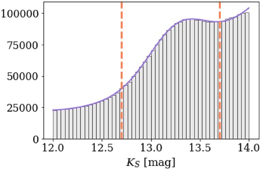
Ks LF around the less reddened RC location of the RGB selected around (J − Ks) = 1. The solid line is fit to the distribution and follows equation (3), and the dashed lines are the adopted limits of the RC selection.
The fitted parameters are |$a=-4.33\times 10^5,~b=1.82\times 10^4,~c=2.6\times 10^6,~\sigma _{\mathrm{ RC}}=0.3\, \mathrm{ mag},~K_s^{\mathrm{ RC}}=13.27$| mag, where σRC = 0.3 mag results from the convolution of the intrinsic width of RC due to the distribution of stellar masses that populate the RC in the observed population (0.2 mag; Alves 2000), the observed width of the RC (0.22 mag; Surot et al. 2019a), and the photometric error from VIRAC2 (∼0.12 mag around the RC). In Fig. 2, the solid line is fit to the Ks LF following equation (3), and the dashed lines mark the limit of the RC selection. The LF for stars around (J − Ks) = 1 peaks at Ks = 13.3 mag. To exclude foreground main-sequence disc stars, we limit the RC selection polygon at the blue end to (J − Ks) ≥ 0.8 mag.
We then refine the selection of the RC candidates by a linear fit to the H − Ks versus J − Ks relation of the stars within the search box (|$-5\deg \lt \, l\lt \, 5\deg$| and |$-3\deg \lt \, b\lt \, 3\deg$|), and selecting ±0.25 mag to the sides of the fit. Fig. 3 shows the H − Ks versus J − Ks diagram, the polygon marks the boundary of the RC selection and the dashed line is the linear fit
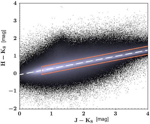
Colour–colour plot covering the 60 deg2 area search box (|$-5\deg \lt \, l\lt \, 5\deg$| and |$-3\deg \lt \, b\lt \, 3\deg$|). The dashed line is the linear fit to refine the RC selection. The box encloses further selection of RC stars.
After selecting the RC region in the CMD and in the colour–colour diagram from VIRAC2, we crossmatch the sources with Gaia DR3 with a 0|${_{.}^{\prime\prime}}$|5 tolerance in position, followed by removing spurious matches, which are identified as outliers in the distributions of (G − Ks) colours.
The mean separation of the crossmatched sources is 0.03 arcsec.
The Gaia DR3 – VIRAC2 matched sample consists of |$2\, 594\, 052$| RC candidate stars within the 60 deg2 region in the inner bulge.
3.1 Foreground decontamination
The principal contaminant of the sample can be M-dwarf stars and reddened main-sequence disc stars and red giant stars from the bulge that populate the same area as the RC stars in the CMD and colour–colour diagrams (Alonso-García et al. 2018; Mejías et al. 2022). Those giant stars, at the faint end of the RC LF, belong to the RGB bump (Nataf et al. 2011), which overlaps with the more distant RC giants tracing the Milky Way structure behind the galactic bar (Gonzalez et al. 2018). Lim et al. (2021) studied the RC population in the southern bulge (|$-6\,$| deg|$\lt \, b \, \lt -9\,$| deg) and found around 25 per cent of RGB bump interlopers in the magnitude range |$13\,$| mag|$\lt \, K_{s_0}\lt \, 14\,$| mag. A spectroscopy follow-up can discern the two populations (e.g. He, Luo & Chen 2022).
Bright foreground stars have well-characterized, reliable parallax in Gaia DR3 and/or in VIRAC2. Hence, we implement a cut in parallax removing those stars that lie within 5 kpc (ϖ > 0.2 mas) and are bright enough to have precise parallax (|$\frac{\sigma _{\varpi }}{\varpi }\lt 0.5$|). However, our sample might still contain faint foreground stars with poorly determined or no parallax measurements in the catalogues. We discuss this further in Section 4.1.
After the parallax cut our sample was reduced from |$2\, 594\, 052$| to |$2\, 077\, 026$| sources.
3.2 Population correction of RC absolute magnitude and distance determination
The absolute magnitude of RC depends on metallicity and age. The brightness of the RC in the Solar neighbourhood is |$M_{K_s}=-1.61$| (Alves et al. 2002; Ruiz-Dern et al. 2018; Sanders et al. 2022). To account for the metallicity and age dependence, a population correction is needed.
The metallicity distribution function (MDF) of RC stars in the bulge is bimodal (Zoccali et al. 2017; Queiroz et al. 2020, 2021; Rojas-Arriagada et al. 2020 ). The peaks are at around [Fe/H] = −0.4 and [Fe/H] = +0.3, with the contributions assumed to be 50 per cent each.3 We take from table 1 of Salaris & Girardi (2002) the stellar evolutionary model theoretical RC magnitudes for metallicity Z = 0.008 and Z = 0.03, corresponding to the two peaks, and average the contributions of these two bulge components to get the mean absolute Ks magnitude ‹|$M_{K_s}$|›.
We also consider three different ages: 8, 10, and 12 Gyr, which are typical of bulge stars (e.g. Surot et al. 2019a; Hasselquist et al. 2020; Sit & Ness 2020). For each age, we take the average ‹|$M_{K_{s_{Z1,Z2}}}$|› given the two metallicity components.
The difference between the local theoretical RC absolute magnitude – i.e. the absolute magnitude of the RC in the stellar evolutionary models of Salaris & Girardi (2002) – and the mean absolute RC magnitude for a given age and metallicity mix is the so-called population correction. It is derived from the Salaris & Girardi (2002) models in the following way:
where |$M_{K_s, \mathrm{ theo}}^{\mathrm{ RC}}=-1.54$|.
The population correction (|$\Delta M_{K_s}^{\mathrm{ RC}}$|) variation between −0.011 and −0.099 mag, depending on age of the bulge RC stars, (see Table 1) is taken as the systematic error in the distance derivation.
Population correction (|$\Delta M_{K_s}^{\mathrm{ RC}}$|) for the Ks absolute magnitude of RC stars. |$\Delta M_{K_s}^{\mathrm{ RC}}$| is computed with table 1 of Salaris & Girardi (2002) assuming different ages and metallicities of Galactic bulge stars.
| Age (Gyr) | Z = 0.008 | Z = 0.03 | |$\Delta M_{K_s}^{\mathrm{ RC}}$| |
|---|---|---|---|
| 8 | −1.446 | −1.611 | −0.011 |
| 10 | −1.385 | −1.571 | −0.062 |
| 12 | −1.309 | −1.572 | −0.099 |
| Age (Gyr) | Z = 0.008 | Z = 0.03 | |$\Delta M_{K_s}^{\mathrm{ RC}}$| |
|---|---|---|---|
| 8 | −1.446 | −1.611 | −0.011 |
| 10 | −1.385 | −1.571 | −0.062 |
| 12 | −1.309 | −1.572 | −0.099 |
The distance modulus μ0 is then
where |$M_{K_s, \mathrm{ obs}.}^{\mathrm{ RC}}$| is the observationally determined absolute Ks magnitude for the local (Solar vicinity) RC population.
To compute the distance, we assume |$M_{K_s, \mathrm{ obs}.}^{\mathrm{ RC}}=-1.61\pm 0.07$| from Sanders et al. (2022), which is in agreement with Ruiz-Dern et al. (2018) |$M_{K_s}=(-1.606\pm 0.009)$|. Then, applying the population correction described above, the distance in pc is expressed as
The heliocentric distances for our selection of RC candidate stars in the bulge CMD range between 7 and 11.5 kpc. For a typical RC star in our sample (Ks = 13.2 mag and extinction of |$A_{K_s}$| = 0.26 mag), the population correction implies a difference in distance of 130 pc compared to the distance derived only using the observed local absolute magnitude (|$M_{K_s}=-1.54$| mag instead of |$M_{K_s}-1.61$| mag).
Adding to that, by assuming different ages, i.e. different corrections, the resulting distances vary by 250 pc, which at the distance of the bulge would be a relative error of 3 per cent. Such value is added to the error budget of the distance distribution.
3.3 Tangential velocity derivation
The high and variable dust extinction towards the Galactic bulge, added to the crowded stellar environment, might cause Gaia DR3 proper motions not be well-characterized (Lindegren et al. 2018; Riello et al. 2021; Fabricius et al. 2021; Battaglia et al. 2022; Luna et al. 2023). For those reasons, we make a separate selection based only on VIRAC2 proper motions, derived from NIR observations, for the following analysis.
After removing the bright foreground objects and having the distance estimation for the RC sources, the VIRAC2 proper motions (|$\mu _{\alpha ^{*}}=\mu _{\alpha } \cos (\delta)$| and μδ) are corrected for the reflex motion of the Sun [(U⊙, V⊙, W⊙) = (12.9, 245.6, 7.78) km s−1] using the gala package (Price-Whelan 2017) from astropy (Astropy Collaboration 2013). For the correction computation we adopt the default Solar motion relative to the GC as a combination for the peculiar velocity (Schönrich, Binney & Dehnen 2010) and for the circular velocity at the Solar radius (Bovy 2015). The tangential velocity of each star in the sample is
where μ is the VIRAC2 proper motion and d is the heliocentric distance.
3.3.1 Monte Carlo sampling
We use a Monte Carlo sampling approach to derive a tangential velocity distribution for each star in our final sample. The VIRAC2 catalogue provides the correlation coefficient between the RA and Dec. components of the proper motions. Together with the proper motion uncertainties, one can use the covariance matrix of each source to generate a multivariate Gaussian distribution of the proper motion errors.
With that, we draw 100 000 random samples of proper motions for each star, which follow a Gaussian distribution. Each of those proper motions is corrected for the reflex motion of the Sun as described in the previous section.
For the distance, we assume a Gaussian distribution with a width given by the following parameters added in quadrature: the photometric error from VIRAC2 (∼0.12 mag around the RC), the absolute magnitude calibration error (0.07 mag; Sanders et al. 2022) and the population correction (0.088 mag; Salaris & Girardi 2002), resulting in a typical distance error of |$\sim 450\,$|pc.
From such distribution, we draw 100 000 random samples of distances for each source. Finally, for each source, we obtain 100 000 samples of tangential velocity, with the median of the distribution being their characteristic tangential velocity and the uncertainties are computed from the 16th and 84th percentile.
4 RESULTS AND DISCUSSION
The Gaia DR3-VIRAC2 crossmatch and foreground decontamination of the sample resulted in 2 077 026 sources located in the RC region of the NIR-CMD. We further restrict the selection of RC candidate stars to a narrower location in the CMD, within 0.3 < (J − Ks)0 < 1 and −0.1 < (H − Ks)0 < 0.4. From those, 49 sources have a lower limit in tangential velocity (16th percentile) above the local escape velocity, with a relative error in their tangential velocities smaller than 30 per cent (|$\frac{\sigma _{V_{\mathrm{ tan}}}}{V_{\mathrm{ tan}}}\, \lt \, 0.3$|) and |$\sigma _{V_{\mathrm{ tan}}}$| the difference between the 16th and 84th percentiles. The local escape velocity depends on the assumed potential, and for the Galactic bulge, it ranges between ∼600 and ∼800 |$\mathrm{km\, s^{-1}}$|, reaching the latter within |$1\,$|kpc of the GC (Rossi et al. 2017; Deason et al. 2019).
To be more inclusive, we adopt the lower limit in velocity as the escape velocity given by the MWPotential2014 Galactic potential from the galpy package (Bovy 2015), with the addition of the influence of the bar – using the DehnenBarPotential from galpy – and a Kepler potential for Sgr A*. The potential is in the low-mass end of the Galaxy mass estimates (Callingham et al. 2019), with a total mass within 60 kpc of |$4\pm 0.7\times 10^{11}\, {\rm M}_{\odot }$| (Xue et al. 2008). In this potential, the dark matter halo is described by a NFW Potential, the bulge is modelled as a power-law density profile with an exponent of −1.8 and a cut-off radius of 1.9 kpc and the disc is modelled with a Miyamoto Nagai potential. The selection of the potential implies that some of the selected candidates move fast, but might still be bound, depending on their exact locations.
Their tangential velocities range between 731 and 1938 |$\mathrm{km\, s^{-1}}$|, and are located between 0.3 and 3.5 kpc from the GC (considered to be at |$R_0=8.122\,$|kpc; GRAVITY Collaboration 2018). The range of tangential velocities is in agreement with the predictions from Generozov (2020) and data from Brown (2015), Boubert et al. (2018), and Koposov et al. (2020).
4.1 Possible sample contaminants and selection of interesting objects
The current data do not have sufficient information to assign a spectral type to each star. A precise spectroscopic determination of the stellar parameters (log g and Teff) and the metallicity will enable us to confirm the stars as RC giants, hence confirming their location in the Galactic bulge.
To refine the sample of RC stars, we identify sources that might be M-dwarfs given their colours. For this, we follow the colour cuts by Mejías et al. (2022), based on a spectroscopically confirmed sample of M-dwarfs by West et al. (2011)
Three sources fall into the selection cuts, placing them as possible M-dwarfs. Their properties are listed in Appendix A. Removing the likely M-dwarfs, the selection results in a sample of 46 stars. The excess of stars in the faint-end of the LF (solid histogram in Fig. 4) is expected. It is a consequence of a larger volume for the more distant, thus fainter, sources in the sample.
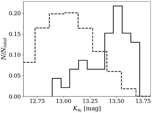
|$K_{s_0}$| LF. The y-axis shows the normalized count of sources. The dashed histogram are the stars within the magnitude range |$12.5\lt K_{s_0}\lt 13.75$|. The solid histogram are the 46 stars that travel with a tangential velocity larger than the local escape velocity and that are not identified as M-dwarfs by their colour.
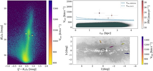
Fig. 5 shows the location of the 46 high-velocity stars in the extinction-corrected NIR CMD.
Deredenned CMD. The circles are stars that travel with a tangential velocity larger than the local escape velocity, colour-coded by their tangential velocity.
Given the heliocentric distance d derived from the RC calibration, we derive the distance with respect to the GC (rGC) using astropy and the following parameters: the International Celestial Reference System (ICRS) coordinates of the GC (RA, Dec.) = (266.4051, −28.936175) deg (Reid & Brunthaler 2004); the velocity of the Sun in Galactocentric Cartesian coordinates (U⊙, V⊙, W⊙) = (12.9, 245.6, 7.78) |$\mathrm{km\, s^{-1}}$| (Reid & Brunthaler 2004; Drimmel & Poggio 2018; GRAVITY Collaboration 2018); the distance from the Sun to the Galactic mid-plane z⊙ = 20.8 pc (Bennett & Bovy 2019), and the distance from the Sun to the GC d⊙ = 8.122 kpc (GRAVITY Collaboration 2018).
Fig. 6 shows the tangential velocity of the stars as a function of the galactocentric distance (rGC). The solid line indicates the escape velocity at a given galactocentric distance, assuming the MWPotential2014 potential from the galpy package (Bovy 2015). The adopted potential is only a reference that helped us to select the threshold in velocity. Different assumptions would change the escape velocity by tens of |$\mathrm{km\, s^{-1}}$|. As a reference for a higher escape velocity profile, the plot also shows the escape velocity profile given by the Irrgang13III potential from the galpy package. This potential is the Model III of Irrgang et al. (2013), with a total Galaxy mass within 50 kpc of |$8.1\times 10^{11}\, {\rm M}_{\odot }$|.
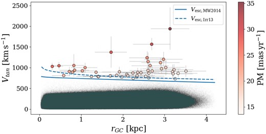
Tangential velocity versus galactocentric distance (rGC). The solid and dashed lines are the escape velocity at a given rGC assuming the galpy Galactic potential MWPotential2014, or Irrgang13III, respectively. The points are the 265 stars remaining after foreground objects’ decontamination, and colour and quality cuts. The points are colour-coded by their VIRAC2 proper motions (PM).
The position in the sky of the final sample is shown in Fig. 7 in galactic coordinates. The background is the density plot of the VIRAC2 sources in the search box, where a whiter colour indicates a higher density, and is equivalent to a reddening map. The arrows represent the VIRAC2 proper motion vectors along the galactic latitude (b) and longitude (l) components, colour-coded by their tangential velocity. Black lines indicate the Gaia DR3 proper motion vector transformed to galactic coordinates and corrected for the reflex motion of the Sun. We note that the Gaia DR3 proper motion of some sources matches with that of VIRAC2, particularly for the sources with slower velocities.
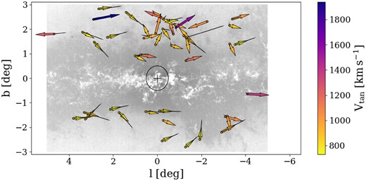
Stars that travel with a tangential velocity larger than the local escape velocity. The arrows represent the VIRAC2 proper motion vectors along the galactic latitude (b) and longitude (l) components after correcting for the reflex motion of the Sun. The points and arrows are colour-coded by the tangential velocity of the source. Black lines indicate the Gaia DR3 proper motion vector transformed to galactic coordinates and corrected for the reflex motion of the Sun. The cross places the GC at (l, b) = (0, 0) and the circle surrounding it represents a radius of |$0.5\deg \simeq 75\,$|pc.
In Fig. 7, we note asymmetries in the spatial distribution and proper motions of the sample. In the initial sample of Gaia DR3 – VIRAC2 crossmatch, the stars are distributed evenly in galactic latitude and longitude. However, in the sample of 46 high-velocity stars, 31 (67 per cent) stars are located at positive galactic latitudes. Furthermore, 39 (85 per cent) stars have VIRAC2 proper motion vectors pointing towards negative galactic longitude.
Based on the Gaia DR3 mock catalogue (Rybizki et al. 2020), a synthetic Milky Way catalogue that simulates the Gaia EDR34 content, within the magnitude and colour range of our sample (17.8 < G < 19.7 mag; 2.6 < BP − RP < 3.9 mag), it is expected that ∼80 per cent of stars lie at a distance between 6.5 and 9.5 kpc. However, some of the stars in our final sample might still be foreground contaminants. Fig. 8 shows the tangential velocity of the stars as a function of their VIRAC2 proper motions. The dashed lines indicate the tangential velocity as a function of the proper motion for different fixed heliocentric distances, while the solid line is at the distance of the GC (8.122 kpc). Even if some of the stars were located at smaller heliocentric distances than our estimates, more than half of them are interesting objects travelling faster than the average disc rotation (246 |$\mathrm{km\, s^{-1}}$|).
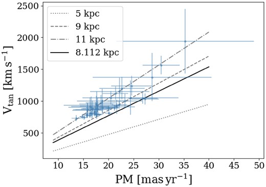
Tangential velocity as a function of proper motion at different fixed heliocentric distances. The points are the 46 high-velocity stars in the sample described in Section 4.1, their proper motions are from VIRAC2 and the tangential velocities are computed with equation (8). The dashed lines indicate the tangential velocity as a function of the proper motion for different fixed heliocentric distances, while the solid line is at the distance of the GC.
4.2 HVSs candidates and flight time
To test whether the HVS candidates radiate from the GC, we project the proper motion vectors, appropriately account for the Solar motion, and search for those that intersect a region within |$0.5\deg$| (∼75 pc at the distance of the GC) centred on the GC. This criterion is based on Speedystar5 (Evans, Marchetti & Rossi 2022b), where we simulate ejections of stars from the GC via the Hills mechanism and analyse the position angle of their proper motions corrected by the reflex motion of the Sun. The stars that are within 4 kpc from the GC, such as the stars in our sample, have a 2D velocity vector (projected proper motion) that approaches the GC in less than 0.45 deg. The criterion also accounts for the uncertainty in the GC distance (31 pc ∼ 0.2 deg), the GC position (0.66 mas; GRAVITY Collaboration 2018, 2021), and encloses the nuclear star cluster (0.03 deg; Schödel et al. 2014, 2023).
There are four sources that fulfil this condition. Their projected 2D velocity vector approaches the GC in a range between |$0.004$| and |$0.47\, \deg$|; since these measurements lack radial velocity, the approach is not a physical quantity. The left panel of Fig. 9 shows their location in the CMD colour-coded by their tangential velocities. The top-right panel shows their tangential velocity as a function of their galactocentric distance colour-coded by their VIRAC2 proper motions, while the bottom-right panel shows their location in galactic coordinates, with the VIRAC2 vectors represented as arrows colour-coded by the tangential velocity.
NIR photometry, position, and kinematics of the candidate HVSs detected in both VIRAC2 and Gaia DR3. Stars that appear to be ejected from within |$0.5\, \deg \simeq 75$| pc of the GC. The left panel is the CMD, the same as in Fig. 5. The top-right panel is the tangential velocity as a function of galactocentric distance, same as Fig. 6. The bottom-right panel is the location of the stars in galactic coordinates with the VIRAC2 proper motions shown as arrows colour-coded by their tangential velocities, same as Fig. 7. In the bottom-right panel, the cross marks the GC, and the surrounding circle has a radius of |$0.5\deg \simeq 75\,$|pc.
To compute how long ago the HVS were ejected from the GC – the flight time, we project the VIRAC2 proper motion vectors backwards, in the direction towards the GC. We assume that the proper motion direction is not strongly affected by the projection in the sky
where tf is the flight time in years, l and b are in degrees and |$\mu =\sqrt{\mu _{l^{*}}^2+\mu _b^2}$| in mas yr−1.
The flight time of these four stars ranges from 1.1 × 10⁶ to 3.2 × 10⁶ yr. We can roughly estimate the ejection rate of RC stars by dividing the number of stars over the range of flight times, this is NHVS/(max(tF) − min(tF)), where NHVS is the observed number of RC HVS candidates, and the denominator is the difference between the maximum and minimum flight time of the candidates. This corresponds to an ejection rate of 1.9 × 10⁻⁶ yr−1. However, we note that this is not a complete sample, and it is limited to the RC mass range, typically between 0.8 and 2 M⊙ (Girardi 2016). Our sample is also affected by contamination from non-RC stars that can only be disentangled with a spectroscopic follow-up. Therefore, the ejection rates are lower than the total integrated rate, which current studies estimate at |$10^{-4}\, \mathrm{ yr}^{-1}$|. This ejection rate estimate depends on the adopted IMF; if the IMF is top-light, the ejection rate can be |$10^{-2}\, \mathrm{ yr}^{-1}$|, but if it is top-heavy, it can be |$10^{-4.5}\, \mathrm{ yr}^{-1}$| (e.g. Rossi et al. 2017; Marchetti, Evans & Rossi 2022; Evans, Marchetti & Rossi 2022a, b).
Table 2 shows for the four stars, the location in equatorial and galactic coordinates, and photometric information (Ks and J − Ks), Table 3 shows their VIRAC2 proper motions, and the derived parameters: tangential velocity (Vtan), galactocentric distance (rGC), flight time (tf), closest approach of the 2D velocity vector to the GC, and the probability (P) of exceeding the escape velocity, given by |$V_{\mathrm{ tan}, 16{\rm th}}(r_{\mathrm{ GC}})/V_{\mathrm{ esc}}(r_{\mathrm{ GC}})$|, with |$V_{\mathrm{ tan}, 16{\rm th}}$| the lower limit in tangential velocity (16th percentile), and Vesc(rGC) given by the galpyIrrgang13III potential; the stars that exceed such escape velocity have a probability of 1.
Location and photometric properties of the stars with Gaia DR3 counterpart and VIRAC2 proper motions pointing away from |$0.5\deg$| around the GC. The Galactic longitude and latitude have a precision of 0|${_{.}^{\prime\prime}}$|5.
| Gaia DR3 source ID | RA (hms) | Dec. (dms) | l (deg) | b (deg) | Ks (mag) | J − Ks (mag) |
|---|---|---|---|---|---|---|
| 4060857768397863040 | 17h39m53|${_{.}^{\rm s}}$|68 | −27d42m35|${_{.}^{\rm s}}$|30 | 0.3801 | 1.7167 | 13.82 | 1.69 |
| 4057025592419323520 | 17h39m43|${_{.}^{\rm s}}$|89 | −29d39m47|${_{.}^{\rm s}}$|42 | −1.2939 | 0.7088 | 14.19 | 2.24 |
| 4058312403271263360 | 17h31m35|${_{.}^{\rm s}}$|90 | −31d10m44|${_{.}^{\rm s}}$|87 | −3.5167 | 1.3669 | 13.62 | 1.3 |
| 4054179029853634816 | 17h38m08|${_{.}^{\rm s}}$|01 | −32d44m09|${_{.}^{\rm s}}$|58 | −4.0754 | −0.6413 | 14.04 | 2.57 |
Derived parameters of the stars with Gaia DR3 counterpart and VIRAC2 proper motions pointing out from |$0.5\deg$| around the GC. The second to last column indicates how close the projected 2D velocity vector approaches the GC. The last column indicates the probability of exceeding the escape velocity.
| Gaia DR3 source ID | μ (|$\mathrm{ mas}\, \mathrm{ yr}^{-1}$|) | d (kpc) | rGC (kpc) | Vtan (|$\mathrm{km\, s^{-1}}$|) | tf (yr) | Approach (deg) | P |
|---|---|---|---|---|---|---|---|
| 4060857768397863040 | 17.77 | 10.46 | 2.36 | 885.15 | 1 501 668 | 0.379 | 1 |
| 4057025592419323520a | 22.25 | 10.72 | 2.6 | 1147.16 | 1 126 034 | 0.297 | 1 |
| 4058312403271263360a | 17.58 | 9.42 | 1.42 | 784.82 | 3 239 459 | 0.165 | 0.94 |
| 4054179029853634816 | 28.69 | 9.72 | 1.72 | 1372.12 | 2 772 852 | 0.369 | 1 |
According to the classifier of spurious astrometric solution in Gaia DR3 (Rybizki et al. 2022), these sources have a good astrometric solution. The VIRAC2 proper motions are consistent within 1σ.
5 THE RED SAMPLE
In this section, we explore those sources that appear in VIRAC2, but not in Gaia DR3, because they are too faint or highly reddened.
We follow the procedure described in Sections 3 and 4, to select the RC stars, and clean the sample of foreground stars including M-dwarfs using VIRAC2 parallax and colour cuts.
The initial sample consists of 8 596 826 sources that are in the VIRAC2 catalogue, but do not have a crossmatch in Gaia DR3. From those, we remove stars closer than 5 kpc to us (ϖ > 0.2) and precise VIRAC2 parallax (|$\frac{\sigma _{\varpi }}{\varpi }\lt 0.5$|). The remaining sample has 8 214 069 sources. We select sources with lower limits in tangential velocity larger than the escape velocity at a given galactocentric distance. The resulting sample has 504 sources from which 481 have a relative error in their tangential velocities smaller than 30 per cent. From those sources, nine are possible M-dwarfs, identified using the colour cuts of equation (9). Thus, the final sample has 472 sources with tangential velocities up to Vtan = 2468 |$\mathrm{km\, s^{-1}}$|. These stars are shown in Fig. 10. The left panel shows the location of the sources in the CMD corrected for extinction. The top-right panel shows the tangential velocity as a function of the galactocentric distance (rGC). The bottom-right panel shows the location of the sources in galactic coordinates, colour-coded by their tangential velocity, and with the proper motion vector shown as arrows.
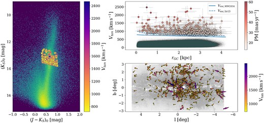
NIR photometry, position, and kinematics of the RC stars detected in VIRAC2, but not in Gaia DR3. The left panel is the CMD, same as in Fig. 5; the top-right panel is the tangential velocity as a function of galactocentric distance, same as Fig. 6; and the bottom-right panel is the location of the stars in galactic coordinates with the VIRAC2 proper motions shown as arrows colour-coded by their tangential velocities, same as Fig. 7.
5.1 HVSs candidates and flight time
Fig. 11 is equivalent to Fig. 10, but shows the stars whose VIRAC2 proper motions point away from the GC. We note that in contrast to Fig. 7, the density of sources is higher towards lower galactic latitudes, where Gaia DR3 has fewer sources. Similar to Fig. 7, 72 per cent of the sources have VIRAC2 proper motions pointing towards negative galactic longitude, but they are distributed evenly in latitude with respect to the Galactic plane.
There are 65 sources that appear to be ejected from a region within |$0.5\deg$| from the GC, with proper motion vectors pointing out of it and with tangential velocities up to Vtan = 1875 |$\mathrm{km\, s^{-1}}$|. Fig. 11 shows the 65 stars.
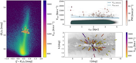
NIR photometry, position, and kinematics of the candidate HVSs detected in VIRAC2, but not in Gaia DR3. Stars that appear to be ejected from within |$0.5\, \mathrm{ deg}\simeq 75\, \mathrm{ pc}$| of the GC. The left panel is the CMD, same as in Fig. 5; the top-right panel is the tangential velocity as a function of galactocentric distance, same as Fig. 6; and the bottom-right panel is the location of the stars in galactic coordinates with the VIRAC2 proper motions shown as arrows colour-coded by their tangential velocities, same as Fig. 7.
Their projected 2D velocity vector approaches the GC in a range between |$0.0004$| and |$0.49\, \deg$|; as mentioned in Section 4.2, these values are not a physical quantity.
Following equation (10), the flight time of the 65 stars appearing to be ejected from the centre ranges between |$2.4\times 10^4$| and |$4.8\times 10^6\, \mathrm{ yr}$|. This provides a rough estimate of an ejection rate of |$1.4\times 10^{-5}\, \mathrm{ yr}^{-1}$|, an order of magnitude higher than for the sample that includes also Gaia DR3 measurements. As explained in Section 4.2, this estimate is lower than the integrated ejection rate. Fig. 12 shows the distribution of flight times, with the major ejection episode occurring before 2 Myr ago.
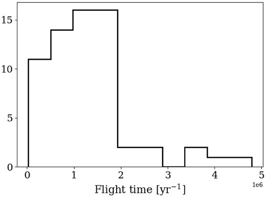
Flight time in Myr for the candidate HVSs that appear in VIRAC2, but not in Gaia DR3 and have a proper motion vector pointing away from a location within |$1 \, \deg \simeq 75$| pc of the GC.
Table 4 is an extract of Table B1 and shows for the 65 stars with VIRAC2 and no Gaia DR3 counterpart, the location in equatorial and galactic coordinates, and photometric information (Ks and J − Ks). Table 5 is an extract of Table B2 and shows VIRAC2 proper motions, and the derived parameters: tangential velocity (Vtan), galactocentric distance (rGC), flight time (tf), the closest approach of the 2D velocity vector to the GC, and the probability (P) of exceeding the escape velocity.
Location and photometric properties of the stars with no Gaia DR3 counterpart and VIRAC2 proper motions pointing away from |$0.5\deg$| around the GC. The Galactic longitude and latitude have a precision of 0|${_{.}^{\prime\prime}}$|5. This is an extract, the complete table can be found in Appendix B.
| ID | RA (hms) | Dec. (dms) | l (deg) | b (deg) | Ks (mag) | J − Ks (mag) |
|---|---|---|---|---|---|---|
| 1 | 17h51m54|${_{.}^{\rm s}}$|16 | −28d01m38|${_{.}^{\rm s}}$|73 | 1.4904 | −0.7146 | 14.28 | 2.26 |
| 2 | 17h49m31|${_{.}^{\rm s}}$|40 | −28d59m43|${_{.}^{\rm s}}$|91 | 0.3911 | −0.7613 | 14.2 | 2.47 |
| 3 | 17h48m40|${_{.}^{\rm s}}$|41 | −29d08m22|${_{.}^{\rm s}}$|46 | 0.172 | −0.6762 | 13.76 | 2.6 |
| 4 | 17h51m11|${_{.}^{\rm s}}$|57 | −28d04m06|${_{.}^{\rm s}}$|82 | 1.375 | −0.6009 | 13.9 | 2.17 |
| 5 | 17h51m33|${_{.}^{\rm s}}$|79 | −27d03m47|${_{.}^{\rm s}}$|14 | 2.2813 | −0.1578 | 14.83 | 3.73 |
| ⋮ | ||||||
Derived parameters of the stars with no Gaia DR3 counterpart and VIRAC2 proper motions pointing out from |$0.5\deg$| around the GC. The second to last column indicates how close the projected 2D velocity vector approaches the GC. The last column is the probability of exceeding the escape velocity. This is an extract, the complete table can be found in Appendix B.
| ID | μ (|$\mathrm{ mas}\, \mathrm{ yr}^{-1}$|) | d (kpc) | rGC (kpc) | Vtan (|$\mathrm{km\, s^{-1}}$|) | tf (yr) | Approach (deg) | P |
|---|---|---|---|---|---|---|---|
| 1 | 19.08 | 11.64 | 3.53 | 1072.9 | 1 362 189 | 0.344 | 1.0 |
| 2 | 19.99 | 10.07 | 1.96 | 982.98 | 68 908 | 0.001 | 0.97 |
| 3 | 26.28 | 7.98 | 0.17 | 1011.28 | 489 957 | 0.234 | 0.86 |
| 4 | 19.82 | 8.9 | 0.81 | 839.35 | 1 213 281 | 0.383 | 0.89 |
| 5 | 16.6 | 10.83 | 2.73 | 856.75 | 2 020 771 | 0.496 | 1.0 |
| ⋮ | |||||||
HVSs can also originate from a globular cluster hosting an intermediate-mass black hole (IMBH). Stellar interactions with the IMBH might result in the ejection of HVSs in a similar way as the Hills mechanism (e.g. Fragione & Gualandris 2019). In that case, the star would point back to its parent cluster.
The spatial and velocity distributions can be used to discern those stars from (hyper)runaway stars originating from the Galactic disc, where the runaway stars have lower velocities and are closer to the Galactic plane (e.g. Fragione & Gualandris 2019; Generozov & Perets 2022). In the same way, the velocity distribution of HVSs originating from the GC would have a larger contribution to high-velocity stars.
A bMBH, like a pair of SMBH–IMBH, would produce HVSs with potentially anisotropic velocity distribution, depending on the eccentricity and mass ratio of the binary stellar system that gets disrupted (e.g. Quinlan 1996; Dotti et al. 2006; Haardt, Sesana & Madau 2006; Sesana, Haardt & Madau 2006). The velocity and spatial distribution predicted by the Hills mechanism are isotropic, thus, the anisotropy in the velocity and spatial distribution of HVSs originating from a bMBH can potentially distinguish their ejection scenario from the SMBH interaction.
The spatial distribution predicted by the Hills mechanism is isotropic. In Fig. 13, we show the position angle (PA) of the sample of 65 stars that point away from the GC. There is a peak in the cos(PA) since most of the stars point towards negative longitudes, but without a trend with velocity (see Fig. 14). Hence, the direction is not isotropic, but the velocity is.
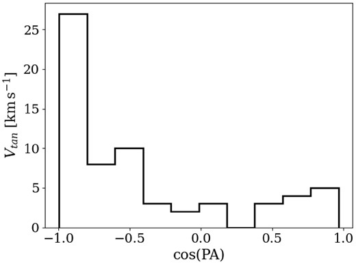
Cosine of the position angle of the stars in VIRAC2 that point out from |$0.5\deg$| around the GC.
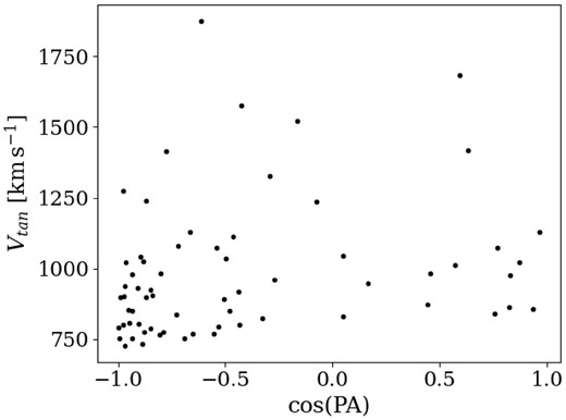
Tangential velocity as a function of the Cosine of the position angle of the stars in VIRAC2 that point out from |$0.5\deg$| around the GC.
Fig. 15 shows the inverse cumulative distribution function of the high-velocity stars’ tangential velocity in both samples: black is the distribution of sources matched in VIRAC2 and Gaia DR3 and that for sources without Gaia DR3 counterpart is plotted with red line. The stars in the sample with only VIRAC2 data are closer to the GC. This sample also contains stars that reach higher velocities than the sample with Gaia DR3 counterpart. With the deceleration occurring in the first |$\sim 200\,$|pc (Kenyon et al. 2008), the stars with Gaia DR3 counterpart, that lie at larger distances from the GC, might have been decelerated.
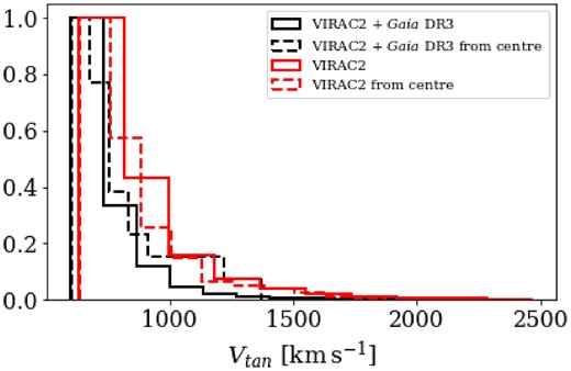
Inverse cumulative distribution of the high-velocity stars. The black histogram is for the final sample of stars in the VIRAC2 and Gaia DR3 crossmatch (solid) and those that point out from |$0.5\deg$| around the GC (dashed). The red histogram is for the final sample of stars in VIRAC2 (solid) and those that point out from |$0.5\deg$| around the GC (dashed).
6 CONCLUSIONS
We have identified 69 HVS candidates in the Milky Way bulge that appear to be ejected from the GC. From those, four have a Gaia DR3 counterpart, but with Gaia proper motions that are not reliable and 65 were detected only in the VIRAC2 sample. All these stars are selected among the likely RC candidates that place them within the bulge. Their flight time ranges between 2.4 × 10⁴ and 4.8 × 10⁶ yr, and implies an integrated ejection rate of the order of 1.4 × 10⁻⁵ yr−1, provided that they all originated from the GC and are currently still within the bulge. Nevertheless, since the surveys are not complete, our sample is not complete. Adding to that, it is limited to RC stars, thus the derived ejection rates are lower than the current estimates (|$10^{-4}\, \mathrm{ yr}^{-1}$|).
To fully determine the HVS candidates’ spatial movement and reconstruct their orbits, we need to obtain the missing radial velocities. The spectroscopic follow-up will also provide the chemical composition and spectral type measurements necessary to confirm the candidates as RC stars. In the case a given star is not an RC star, the distance estimation would not be correct, nor its tangential velocity. However, such stars might be still interesting as they would be moving faster than the average disc rotation. Hence, they would offer the possibility of exploring the production scenarios of such stars through e.g. binary interactions or supernova kicks.
Having the first detection of HVSs in the Galactic bulge confirmed by future spectroscopy, we will be in a position to constrain the existing models, compare the observed with HVSs mock population (Marchetti et al. 2018) and compute their orbits (e.g. Fernández-Trincado et al. 2020; GravPot166), and thus probe if they come from the GC or have another origin.
The Hills mechanism is parametrized by the shape of the stellar initial mass function in the GC, the distribution of binary orbital periods and mass fraction, and the ejection rate. The number of confirmed HVSs and their properties will constrain primarily the ejection rate and the shape of the IMF in the adopted model (e.g. Evans, Marchetti & Rossi 2022b, Speedystar). Interestingly, the discovery of the first HVSs close to the production centre will give a unique possibility to explore a recent stellar interaction with Sgr A*.
The velocity distribution is compatible with current ejection models, where the high-velocity stars should reside close to the GC, and those ejected with the Hills mechanism will also have an isotropic spatial distribution. A different spatial distribution, or proper motions that do not point back to the GC can be explained by other ejection scenarios, such as a disruption of globular clusters by the SMBH, inspiralling IMBH, dynamic interactions with binary massive BH, or supernova kicks. The high-velocity stars point back to the production origin, being these globular clusters, satellite galaxies such as the Magellanic Clouds, or the Galactic disc, where the runaway scenario is more probable.
The future Gaia data releases7 will improve the astrometry precision by a factor of ∼2.5, reaching 0.5 and 0.3 mas yr−1 in DR4 and DR5, respectively, for the faintest stars (G = 20.7 mag). The accuracy will improve as well, as the baseline of observations will increase to 60 months in DR4 and 120 months in DR5. The radial velocities are limited to sources brighter than G ∼ 15.5 mag and the spectra at G ∼ 17.5 mag. Thus, to confirm the nature of the candidate HVSs in the Galactic bulge, a dedicated NIR spectroscopic follow-up is still necessary. GaiaNIR is a proposed space mission that will map the entire sky in the NIR, extending the capabilities and deepness of Gaia; if accepted, it will be launched in the 2040s, extending the baseline by 20 yr, which translates into a 20 × more accurate proper motions. The future ground and space facilities might change that scenario. The Extremely Large Telescope (ELT) will reach μas yr−1 precision in proper motions (Trippe et al. 2010; Rodeghiero et al. 2021), and there are JWST observations focusing on the Galactic bulge. The Wide-Field Instrument onboard the Roman telescope will be ideal for NIR surveys with precise photometry (PSF full width at half-maximum <0.1 arcsec) and low resolution (R ∼ 600) multi-object spectroscopy, sufficient for radial velocity measurements. The Rubin observatory will map the southern sky and will reach proper motion precision of 0.2(1) mas yr−1 for sources with magnitude r = 21(24) mag.8
ACKNOWLEDGEMENTS
AL acknowledges support from the Agencia Nacional de Investigación y Desarrollo (ANID) Doctorado Nacional 2021 scholarship 21211520, and the ESO studentship. NWCL gratefully acknowledges the generous support of a Fondo Nacional de Desarrollo Científico y Tecnológico (FONDECYT) regular grant number1230082, as well as support from Millenium Nucleus NCN19_058 (TITANs) and funding via the BASAL Centro de Excelencia en Astrofisica y Tecnologias Afines (CATA) grant PFB-06/2007. NWCL also thanks for support from ANID BASAL project number ACE210002 and ANID BASAL project numbers ACE210002 and FB210003. JA-G acknowledges support from FONDECYT regular grant number 1201490 and ANID – Millennium Science Initiative Program – ICN12_009 awarded to the Millennium Institute of Astrophysics MAS. AVN acknowledges support from the ANID scholarship programme Doctorado Nacional 2020-21201226, ANID, Millennium Science Initiative, ICN12_009 and ANID BASAL FB210003. DM gratefully acknowledges support by the ANID BASAL project numbers ACE210002 and FB210003, by FONDECYT project number 1220724, and by CNPq/Brazil through project number 350104/2022-0. We gratefully acknowledge the use of data from the ESO Public Survey programme IDs 179.B-2002 and 198.B-2004 taken with the VISTA telescope and data products from the Cambridge Astronomical Survey Unit. Funding for the DPAC has been provided by national institutions, in particular, the institutions participating in the Gaia Multilateral Agreement. This research made use of astropy, a community-developed core python package for astronomy (Astropy Collaboration 2013, 2018). This research made use of numpy (Harris et al. 2020), scipy (Virtanen et al. 2020), and scikit-learn (Pedregosa et al. 2011).
DATA AVAILABILITY
We use data from the ESO Public Survey programme IDs 179.B-2002 and 198.B-2004 taken with the VISTA telescope and data products from the Cambridge Astronomical Survey Unit. The VVV reduced images are available in the ESO Science Archive. This work has made use of data from the European Space Agency (ESA) mission Gaia (https://www.cosmos.esa.int/gaia), processed by the Gaia Data Processing and Analysis Consortium (DPAC, https://www.cosmos.esa.int/web/gaia/dpac/consortium). For the HVS candidates, we provide tables in the paper that will be available in CDS.
Footnotes
The stars within 0.01 pc of the GC, namely the S-cluster, are young B-type stars, with ages consistent with the HVSs detected and confirmed in the Galactic halo, supporting the origin scenario of both HVSs and the S-stars.
There are between ∼100 and 300 Ks-band epochs per tile in the Milky Way central regions of the VVV.
The fractional contribution of metal-rich versus metal-poor population depends on Galactic latitude (e.g. Zoccali et al. 2017), but this variation results in distance modulus difference of only ∼0.005 mag.
Gaia EDR3 refers to the early data release, which contains the same astrometric and photometric information as DR3.
References
APPENDIX A: POSSIBLE M-DWARFS IN THE Gaia DR3 – VIRAC2 CROSSMATCH
In this section, we present the list of the possible M-dwarfs in our Gaia DR3 – VIRAC2 sample (Table A1) and in the VIRAC2 sample without Gaia DR3 counterparts (Table A2). These stars are selected with the colour cuts of equation (9), as described in Section 4.1.
Properties of the stars, in the Gaia DR3 – VIRAC2 crossmatch, that could be M-dwarfs according to the colour cuts of equation (9). The proper motions are from VIRAC2, without the reflex motion correction.
| Gaia DR3 source ID | RA (hms) | Dec. (dms) | H (mag) | J (mag) | Ks (mag) | μRA (|$\mathrm{ mas}\, \mathrm{ yr}^{-1}$|) | μDec (|$\mathrm{ mas}\, \mathrm{ yr}^{-1}$|) |
|---|---|---|---|---|---|---|---|
| 4062689730907384576 | 17h59m46|${_{.}^{\rm s}}$|35 | −28d17m16|${_{.}^{\rm s}}$|22 | 13.77 | 14.41 | 13.58 | −13.8 ± 0.25 | −14.39 ± 0.25 |
| 4056600017090916864 | 17h53m44|${_{.}^{\rm s}}$|06 | −29d05m13|${_{.}^{\rm s}}$|19 | 13.67 | 14.28 | 13.45 | 3.21 ± 1.45 | −36.8 ± 1.45 |
| 4043668347447008512 | 17h54m29|${_{.}^{\rm s}}$|02 | −31d27m13|${_{.}^{\rm s}}$|07 | 13.69 | 14.37 | 13.47 | −23.66 ± 0.57 | −5.78 ± 0.57 |
Properties of the stars, in VIRAC2 without Gaia DR3 counterpart, that could be M-dwarfs according to the colour cuts of equation (9). The proper motions are from VIRAC2, without the reflex motion correction.
| RA (hms) | Dec. (dms) | H (mag) | J (mag) | Ks (mag) | μRA (|$\mathrm{ mas}\, \mathrm{ yr}^{-1}$|) | μDec (|$\mathrm{ mas}\, \mathrm{ yr}^{-1}$|) |
|---|---|---|---|---|---|---|
| 17h54m40|${_{.}^{\rm s}}$|43 | −29d36m24|${_{.}^{\rm s}}$|30 | 12.98 | 13.63 | 12.76 | 11.97 ± 0.3 | 15.08 ± 0.3 |
| 17h53m44|${_{.}^{\rm s}}$|06 | −29d05m13|${_{.}^{\rm s}}$|19 | 13.67 | 14.28 | 13.45 | 3.21 ± 1.45 | −36.8 ± 1.45 |
| 17h58m39|${_{.}^{\rm s}}$|42 | −28d45m03|${_{.}^{\rm s}}$|90 | 13.6 | 14.21 | 13.41 | −1.19 ± 0.35 | −46.27 ± 0.35 |
| 18h00m13|${_{.}^{\rm s}}$|95 | −28d37m12|${_{.}^{\rm s}}$|03 | 13.83 | 14.44 | 13.61 | −12.73 ± 0.49 | −15.64 ± 0.49 |
| 17h54m10|${_{.}^{\rm s}}$|59 | −28d51m53|${_{.}^{\rm s}}$|11 | 13.7 | 14.28 | 13.47 | −4.12 ± 1.42 | −37.53 ± 1.42 |
| 18h00m56|${_{.}^{\rm s}}$|51 | −28d26m31|${_{.}^{\rm s}}$|33 | 13.79 | 14.4 | 13.58 | 10.95 ± 0.38 | −12.65 ± 0.38 |
| 18h03m07|${_{.}^{\rm s}}$|61 | −27d19m08|${_{.}^{\rm s}}$|33 | 13.4 | 14.05 | 13.25 | 16.96 ± 0.27 | −14.07 ± 0.27 |
| 17h55m37|${_{.}^{\rm s}}$|24 | −29d48m07|${_{.}^{\rm s}}$|30 | 13.75 | 14.44 | 13.54 | 4.44 ± 0.31 | −23.15 ± 0.31 |
| 17h54m29|${_{.}^{\rm s}}$|02 | −31d27m13|${_{.}^{\rm s}}$|07 | 13.69 | 14.37 | 13.47 | −23.66 ± 0.57 | −5.78 ± 0.57 |
APPENDIX B: STARS IN VIRAC2 POINTING AWAY FROM THE GC
This section presents the photometric properties and derived parameters of the 65 stars that have VIRAC2 data, but no Gaia DR3 counterpart, and whose VIRAC2 proper motions point away from |$0.5\deg$| from the GC.
Location and photometric properties of the stars with no Gaia DR3 counterpart and VIRAC2 proper motions pointing away from |$0.5\deg$| around the GC. The Galactic longitude and latitude have a precision of 0|${_{.}^{\prime\prime}}$|5.
| ID | RA (hms) | Dec. (dms) | l (deg) | b (deg) | Ks (mag) | J − Ks (mag) |
|---|---|---|---|---|---|---|
| 1 | 17h51m54|${_{.}^{\rm s}}$|16 | −28d01m38|${_{.}^{\rm s}}$|73 | 1.4904 | −0.7146 | 14.28 | 2.26 |
| 2 | 17h49m31|${_{.}^{\rm s}}$|40 | −28d59m43|${_{.}^{\rm s}}$|91 | 0.3911 | −0.7613 | 14.2 | 2.47 |
| 3 | 17h48m40|${_{.}^{\rm s}}$|41 | −29d08m22|${_{.}^{\rm s}}$|46 | 0.172 | −0.6762 | 13.76 | 2.6 |
| 4 | 17h51m11|${_{.}^{\rm s}}$|57 | −28d04m06|${_{.}^{\rm s}}$|82 | 1.375 | −0.6009 | 13.9 | 2.17 |
| 5 | 17h51m33|${_{.}^{\rm s}}$|79 | −27d03m47|${_{.}^{\rm s}}$|14 | 2.2813 | −0.1578 | 14.83 | 3.73 |
| 6 | 17h48m37|${_{.}^{\rm s}}$|10 | −28d56m04|${_{.}^{\rm s}}$|77 | 0.3413 | −0.5602 | 14.52 | 3.27 |
| 7 | 17h46m56|${_{.}^{\rm s}}$|33 | −26d52m27|${_{.}^{\rm s}}$|36 | 1.913 | 0.8229 | 13.92 | 1.8 |
| 8 | 17h46m20|${_{.}^{\rm s}}$|34 | −28d08m31|${_{.}^{\rm s}}$|05 | 0.7604 | 0.2784 | 14.45 | 2.85 |
| 9 | 17h45m13|${_{.}^{\rm s}}$|27 | −28d31m47|${_{.}^{\rm s}}$|60 | 0.3011 | 0.2864 | 14.72 | 3.67 |
| 10 | 17h42m02|${_{.}^{\rm s}}$|43 | −27d46m11|${_{.}^{\rm s}}$|88 | 0.5804 | 1.2819 | 14.0 | 1.73 |
| 11 | 17h46m06|${_{.}^{\rm s}}$|37 | −27d50m16|${_{.}^{\rm s}}$|34 | 0.9934 | 0.4805 | 14.61 | 3.15 |
| 12 | 17h46m40|${_{.}^{\rm s}}$|54 | −27d40m40|${_{.}^{\rm s}}$|52 | 1.1956 | 0.4559 | 14.86 | 3.96 |
| 13 | 17h41m25|${_{.}^{\rm s}}$|95 | −26d49m12|${_{.}^{\rm s}}$|87 | 1.3162 | 1.8978 | 14.14 | 1.99 |
| 14 | 17h42m14|${_{.}^{\rm s}}$|52 | −27d48m39|${_{.}^{\rm s}}$|42 | 0.5691 | 1.2225 | 14.02 | 1.92 |
| 15 | 17h45m18|${_{.}^{\rm s}}$|18 | −28d00m29|${_{.}^{\rm s}}$|66 | 0.7556 | 0.5432 | 14.61 | 3.06 |
| 16 | 17h43m10|${_{.}^{\rm s}}$|80 | −29d03m55|${_{.}^{\rm s}}$|52 | −0.3893 | 0.387 | 15.05 | 3.86 |
| 17 | 17h41m30|${_{.}^{\rm s}}$|29 | −29d16m18|${_{.}^{\rm s}}$|41 | −0.7574 | 0.589 | 15.17 | 4.22 |
| 18 | 17h40m51|${_{.}^{\rm s}}$|43 | −29d53m26|${_{.}^{\rm s}}$|62 | −1.3571 | 0.381 | 14.47 | 2.58 |
| 19 | 17h42m56|${_{.}^{\rm s}}$|86 | −28d47m26|${_{.}^{\rm s}}$|55 | −0.1823 | 0.5747 | 14.41 | 3.63 |
| 20 | 17h40m42|${_{.}^{\rm s}}$|81 | −29d54m45|${_{.}^{\rm s}}$|52 | −1.3922 | 0.3958 | 14.4 | 2.34 |
| 21 | 17h42m12|${_{.}^{\rm s}}$|50 | −28d57m57|${_{.}^{\rm s}}$|80 | −0.4166 | 0.62 | 14.58 | 2.79 |
| 22 | 17h28m51|${_{.}^{\rm s}}$|23 | −32d26m46|${_{.}^{\rm s}}$|33 | −4.8958 | 1.1563 | 14.39 | 2.3 |
| 23 | 17h44m12|${_{.}^{\rm s}}$|97 | −28d58m25|${_{.}^{\rm s}}$|90 | −0.1925 | 0.2422 | 15.17 | 4.25 |
| 24 | 17h41m47|${_{.}^{\rm s}}$|24 | −29d51m26|${_{.}^{\rm s}}$|34 | −1.2221 | 0.2276 | 14.79 | 3.58 |
| 25 | 17h40m18|${_{.}^{\rm s}}$|47 | −30d17m17|${_{.}^{\rm s}}$|94 | −1.7572 | 0.2709 | 14.39 | 3.05 |
| 26 | 17h37m08|${_{.}^{\rm s}}$|53 | −30d54m12|${_{.}^{\rm s}}$|78 | −2.6411 | 0.5185 | 14.7 | 3.06 |
| 27 | 17h43m48|${_{.}^{\rm s}}$|93 | −28d41m41|${_{.}^{\rm s}}$|24 | −0.0008 | 0.4631 | 14.52 | 3.06 |
| 28 | 17h34m24|${_{.}^{\rm s}}$|30 | −30d25m27|${_{.}^{\rm s}}$|57 | −2.5551 | 1.2727 | 13.89 | 1.36 |
| 29 | 17h38m49|${_{.}^{\rm s}}$|22 | −29d59m14|${_{.}^{\rm s}}$|81 | −1.6737 | 0.7033 | 14.21 | 1.99 |
| 30 | 17h35m55|${_{.}^{\rm s}}$|31 | −28d38m22|${_{.}^{\rm s}}$|47 | −0.8743 | 1.9593 | 13.83 | 1.35 |
| 31 | 17h44m04|${_{.}^{\rm s}}$|72 | −29d02m36|${_{.}^{\rm s}}$|47 | −0.2676 | 0.2313 | 14.76 | 3.7 |
| 32 | 17h44m04|${_{.}^{\rm s}}$|69 | −29d09m25|${_{.}^{\rm s}}$|08 | −0.3643 | 0.172 | 15.01 | 3.84 |
| 33 | 17h40m15|${_{.}^{\rm s}}$|79 | −29d57m06|${_{.}^{\rm s}}$|96 | −1.4773 | 0.4577 | 14.38 | 2.61 |
| 34 | 17h40m56|${_{.}^{\rm s}}$|25 | −29d10m23|${_{.}^{\rm s}}$|60 | −0.7392 | 0.7462 | 14.71 | 3.09 |
| 35 | 17h43m29|${_{.}^{\rm s}}$|07 | −29d13m15|${_{.}^{\rm s}}$|07 | −0.4866 | 0.2488 | 15.01 | 3.97 |
| 36 | 17h40m17|${_{.}^{\rm s}}$|31 | −30d23m30|${_{.}^{\rm s}}$|21 | −1.8471 | 0.2196 | 14.62 | 3.43 |
| 37 | 17h32m26|${_{.}^{\rm s}}$|70 | −29d35m51|${_{.}^{\rm s}}$|44 | −2.0918 | 2.0782 | 13.84 | 1.55 |
| 38 | 17h40m49|${_{.}^{\rm s}}$|56 | −29d05m33|${_{.}^{\rm s}}$|27 | −0.6837 | 0.8096 | 14.5 | 2.55 |
| 39 | 17h43m04|${_{.}^{\rm s}}$|90 | −29d48m44|${_{.}^{\rm s}}$|04 | −1.0359 | 0.0127 | 15.2 | 4.31 |
| 40 | 17h41m51|${_{.}^{\rm s}}$|13 | −29d41m08|${_{.}^{\rm s}}$|00 | −1.0688 | 0.3063 | 15.06 | 3.91 |
| 41 | 17h45m47|${_{.}^{\rm s}}$|85 | −28d57m43|${_{.}^{\rm s}}$|36 | −0.0019 | −0.0466 | 14.58 | 4.74 |
| 42 | 17h45m40|${_{.}^{\rm s}}$|89 | −30d57m20|${_{.}^{\rm s}}$|09 | −1.717 | −1.0633 | 14.51 | 2.73 |
| 43 | 17h43m56|${_{.}^{\rm s}}$|25 | −30d27m16|${_{.}^{\rm s}}$|10 | −1.4854 | −0.4819 | 14.84 | 3.73 |
| 44 | 17h44m41|${_{.}^{\rm s}}$|96 | −30d50m34|${_{.}^{\rm s}}$|58 | −1.7307 | −0.8248 | 15.08 | 4.06 |
| 45 | 17h53m36|${_{.}^{\rm s}}$|27 | −30d32m25|${_{.}^{\rm s}}$|42 | −0.4863 | −2.311 | 13.4 | 1.24 |
| 46 | 17h43m22|${_{.}^{\rm s}}$|40 | −30d52m13|${_{.}^{\rm s}}$|52 | −1.9032 | −0.5967 | 14.97 | 3.91 |
| 47 | 17h44m57|${_{.}^{\rm s}}$|45 | −30d50m45|${_{.}^{\rm s}}$|38 | −1.7044 | −0.8736 | 14.48 | 3.17 |
| 48 | 17h47m09|${_{.}^{\rm s}}$|07 | −32d46m43|${_{.}^{\rm s}}$|90 | −3.1142 | −2.2762 | 13.89 | 1.46 |
| 49 | 17h45m27|${_{.}^{\rm s}}$|22 | −30d08m00|${_{.}^{\rm s}}$|62 | −1.0408 | −0.5931 | 14.99 | 3.89 |
| 50 | 17h48m34|${_{.}^{\rm s}}$|48 | −29d33m48|${_{.}^{\rm s}}$|56 | −0.2024 | −0.8763 | 14.21 | 2.09 |
| 51 | 17h43m16|${_{.}^{\rm s}}$|85 | −32d48m15|${_{.}^{\rm s}}$|56 | −3.5599 | −1.5952 | 13.98 | 1.52 |
| 52 | 17h44m50|${_{.}^{\rm s}}$|13 | −30d55m19|${_{.}^{\rm s}}$|86 | −1.7831 | −0.8911 | 14.64 | 3.34 |
| 53 | 17h46m07|${_{.}^{\rm s}}$|04 | −30d51m52|${_{.}^{\rm s}}$|92 | −1.5907 | −1.0958 | 14.29 | 2.23 |
| 54 | 17h45m27|${_{.}^{\rm s}}$|17 | −29d12m17|${_{.}^{\rm s}}$|06 | −0.2482 | −0.1088 | 14.44 | 4.14 |
| 55 | 17h46m33|${_{.}^{\rm s}}$|01 | −29d25m09|${_{.}^{\rm s}}$|19 | −0.3069 | −0.4247 | 14.96 | 3.7 |
| 56 | 17h46m02|${_{.}^{\rm s}}$|56 | −30d00m09|${_{.}^{\rm s}}$|59 | −0.8627 | −0.6338 | 14.97 | 3.82 |
| 57 | 17h44m45|${_{.}^{\rm s}}$|93 | −30d20m20|${_{.}^{\rm s}}$|38 | −1.2936 | −0.5736 | 15.02 | 3.83 |
| 58 | 17h46m17|${_{.}^{\rm s}}$|57 | −30d41m58|${_{.}^{\rm s}}$|40 | −1.43 | −1.0422 | 14.4 | 3.23 |
| 59 | 17h47m08|${_{.}^{\rm s}}$|69 | −29d22m38|${_{.}^{\rm s}}$|78 | −0.204 | −0.5137 | 14.81 | 3.47 |
| 60 | 17h38m42|${_{.}^{\rm s}}$|34 | −33d15m48|${_{.}^{\rm s}}$|34 | −4.4571 | −1.0246 | 14.14 | 1.77 |
| 61 | 17h47m50|${_{.}^{\rm s}}$|76 | −29d41m50|${_{.}^{\rm s}}$|15 | −0.3987 | −0.8098 | 14.06 | 2.77 |
| 62 | 17h47m18|${_{.}^{\rm s}}$|44 | −30d47m53|${_{.}^{\rm s}}$|38 | −1.4012 | −1.2797 | 14.26 | 2.13 |
| 63 | 17h46m57|${_{.}^{\rm s}}$|49 | −29d41m40|${_{.}^{\rm s}}$|51 | −0.4963 | −0.6434 | 14.62 | 3.36 |
| 64 | 17h46m36|${_{.}^{\rm s}}$|58 | −30d34m58|${_{.}^{\rm s}}$|63 | −1.2949 | −1.0399 | 14.39 | 2.66 |
| 65 | 17h42m19|${_{.}^{\rm s}}$|02 | −31d10m41|${_{.}^{\rm s}}$|50 | −2.2841 | −0.5662 | 14.7 | 3.23 |
Derived parameters of the stars with no Gaia DR3 counterpart and VIRAC2 proper motions pointing out from |$0.5\deg$| around the GC. The second to last column indicates how close the projected 2D velocity vector approaches the GC. The last column is the probability of exceeding the escape velocity.
| ID | μ (|$\mathrm{ mas}\, \mathrm{ yr}^{-1}$|) | d (kpc) | rGC (kpc) | Vtan (|$\mathrm{km\, s^{-1}}$|) | tf (yr) | Approach (deg) | |
|---|---|---|---|---|---|---|---|
| 1 | 19.08 | 11.64 | 3.53 | 1072.9 | 1362189 | 0.344 | 1.0 |
| 2 | 19.99 | 10.07 | 1.96 | 982.98 | 68908 | 0.001 | 0.97 |
| 3 | 26.28 | 7.98 | 0.17 | 1011.28 | 489957 | 0.234 | 0.86 |
| 4 | 19.82 | 8.9 | 0.81 | 839.35 | 1213281 | 0.383 | 0.89 |
| 5 | 16.6 | 10.83 | 2.73 | 856.75 | 2020771 | 0.496 | 1.0 |
| 6 | 17.33 | 10.1 | 1.98 | 830.76 | 567325 | 0.293 | 0.98 |
| 7 | 20.07 | 10.06 | 1.96 | 978.06 | 1673409 | 0.32 | 0.97 |
| 8 | 22.83 | 10.09 | 1.97 | 1128.96 | 610088 | 0.069 | 1.0 |
| 9 | 21.35 | 10.17 | 2.05 | 1044.98 | 32379 | 0.279 | 1.0 |
| 10 | 16.58 | 11.0 | 2.89 | 871.98 | 124411 | 0.041 | 1.0 |
| 11 | 19.51 | 10.6 | 2.48 | 1021.4 | 899316 | 0.06 | 1.0 |
| 12 | 16.93 | 10.5 | 2.38 | 863.32 | 1119425 | 0.26 | 0.92 |
| 13 | 31.41 | 11.08 | 2.99 | 1683.19 | 1483537 | 0.055 | 1.0 |
| 14 | 18.24 | 10.77 | 2.65 | 947.92 | 1136668 | 0.31 | 1.0 |
| 15 | 28.29 | 10.56 | 2.44 | 1418.33 | 62984 | 0.228 | 1.0 |
| 16 | 14.64 | 11.7 | 3.58 | 823.63 | 516474 | 0.225 | 0.93 |
| 17 | 16.33 | 11.5 | 3.39 | 899.95 | 854837 | 0.122 | 1.0 |
| 18 | 17.4 | 11.61 | 3.5 | 979.57 | 1216416 | 0.108 | 1.0 |
| 19 | 21.66 | 9.27 | 1.15 | 960.71 | 466379 | 0.018 | 0.98 |
| 20 | 17.45 | 10.77 | 2.65 | 906.58 | 1247434 | 0.358 | 0.98 |
| 21 | 14.3 | 11.39 | 3.27 | 774.61 | 711158 | 0.209 | 0.95 |
| 22 | 14.27 | 10.75 | 2.76 | 727.1 | 4794263 | 0.034 | 0.93 |
| 23 | 15.41 | 10.82 | 2.7 | 794.32 | 283765 | 0.033 | 0.93 |
| 24 | 14.52 | 11.37 | 3.26 | 788.06 | 1174594 | 0.385 | 0.92 |
| 25 | 19.44 | 9.72 | 1.62 | 898.35 | 1451589 | 0.034 | 1.0 |
| 26 | 13.51 | 11.76 | 3.67 | 752.89 | 2636652 | 0.126 | 0.98 |
| 27 | 22.91 | 10.14 | 2.01 | 1112.38 | 348364 | 0.206 | 1.0 |
| 28 | 16.36 | 10.86 | 2.78 | 853.39 | 2540906 | 0.297 | 0.94 |
| 29 | 15.64 | 10.76 | 2.66 | 800.31 | 1652376 | 0.267 | 0.95 |
| 30 | 18.3 | 10.53 | 2.44 | 917.74 | 1805352 | 0.056 | 1.0 |
| 31 | 25.02 | 10.35 | 2.23 | 1240.06 | 254584 | 0.068 | 1.0 |
| 32 | 28.88 | 11.31 | 3.19 | 1576.01 | 269883 | 0.251 | 1.0 |
| 33 | 16.68 | 11.32 | 3.21 | 900.49 | 1363378 | 0.089 | 1.0 |
| 34 | 15.38 | 11.51 | 3.39 | 850.99 | 964212 | 0.252 | 0.96 |
| 35 | 15.42 | 10.93 | 2.81 | 800.31 | 500993 | 0.311 | 0.97 |
| 36 | 15.99 | 10.6 | 2.5 | 807.72 | 1674628 | 0.313 | 0.94 |
| 37 | 21.79 | 10.57 | 2.49 | 1127.72 | 2274099 | 0.143 | 1.0 |
| 38 | 14.32 | 11.3 | 3.19 | 770.23 | 1008236 | 0.007 | 0.93 |
| 39 | 13.14 | 11.76 | 3.64 | 733.39 | 1028925 | 0.407 | 0.92 |
| 40 | 15.15 | 10.98 | 2.87 | 791.94 | 1028237 | 0.19 | 0.96 |
| 41 | 47.89 | 8.24 | 0.12 | 1875.12 | 24273 | 0.027 | 1.0 |
| 42 | 17.44 | 11.84 | 3.73 | 983.76 | 1741107 | 0.137 | 1.0 |
| 43 | 18.43 | 10.56 | 2.45 | 925.84 | 1309472 | 0.316 | 1.0 |
| 44 | 17.11 | 11.39 | 3.29 | 929.66 | 1668731 | 0.028 | 1.0 |
| 45 | 30.39 | 9.15 | 1.09 | 1325.27 | 1542188 | 0.176 | 1.0 |
| 46 | 20.7 | 10.38 | 2.28 | 1022.51 | 1578184 | 0.058 | 1.0 |
| 47 | 21.18 | 9.97 | 1.87 | 1024.82 | 1498155 | 0.03 | 1.0 |
| 48 | 15.51 | 10.27 | 2.23 | 754.23 | 3526367 | 0.411 | 0.94 |
| 49 | 25.96 | 11.41 | 3.3 | 1413.54 | 846379 | 0.183 | 1.0 |
| 50 | 17.76 | 10.54 | 2.42 | 893.5 | 768377 | 0.245 | 1.0 |
| 51 | 14.75 | 10.78 | 2.73 | 753.78 | 3656984 | 0.128 | 0.95 |
| 52 | 20.11 | 10.97 | 2.87 | 1079.99 | 1600298 | 0.496 | 1.0 |
| 53 | 20.14 | 10.84 | 2.74 | 1041.09 | 1549381 | 0.231 | 1.0 |
| 54 | 39.51 | 8.12 | 0.04 | 1520.99 | 155229 | 0.226 | 1.0 |
| 55 | 23.87 | 10.71 | 2.59 | 1234.92 | 386132 | 0.264 | 1.0 |
| 56 | 14.22 | 11.37 | 3.25 | 766.62 | 1021822 | 0.0 | 0.99 |
| 57 | 16.58 | 10.62 | 2.51 | 836.06 | 1250916 | 0.396 | 1.0 |
| 58 | 17.12 | 9.89 | 1.79 | 803.86 | 1539368 | 0.265 | 0.95 |
| 59 | 14.31 | 11.28 | 3.16 | 769.73 | 526093 | 0.105 | 0.93 |
| 60 | 15.52 | 11.42 | 3.39 | 848.9 | 4179327 | 0.357 | 0.99 |
| 61 | 23.63 | 9.27 | 1.16 | 1073.24 | 668479 | 0.096 | 1.0 |
| 62 | 19.26 | 11.06 | 2.96 | 1036.36 | 155673 | 0.481 | 1.0 |
| 63 | 18.39 | 10.47 | 2.35 | 938.49 | 682123 | 0.466 | 0.97 |
| 64 | 15.11 | 10.79 | 2.68 | 774.97 | 1538132 | 0.237 | 0.93 |
| 65 | 23.2 | 11.24 | 3.15 | 1274.34 | 1758733 | 0.06 | 1.0 |
