


ABSTRACT
We present a long-term X-ray study of a nearby Active Galactic Nucleus Mrk 6, utilizing observations from XMM–Newton, Suzaku, Swift, and NuSTAR observatories, spanning 22 years from 2001 to 2022. From timing analysis, we estimated variance, normalized variance, and fractional rms amplitude in different energy bands.The temporal study shows fractional rms amplitude (Fvar) below 10 per cent for the shorter time-scale (∼60 ks) and above 20 per cent for the longer time-scale (∼weeks). A complex correlation is observed between the soft (0.5–3.0 keV) and hard (3.0–10.0 keV) X-ray bands of different epochs of observations. This result prompts a detailed investigation through spectral analysis, employing various phenomenological and physical models on the X-ray spectra. Our analysis reveals a heterogeneous structure of the obscuring material surrounding Mrk 6. A partially ionized absorber exhibits a rapid change in location and extends up to the narrow-line regions or torus. In contrast, another component, located far from the central engine, remained relatively stable. During the observation period, the source luminosity in the 3.0–10.0 keV range varies between (3–15) × 1042 erg s−1.
1 INTRODUCTION
Active Galactic Nuclei (AGNs) are the extremely luminous and most persistent energetic sources in the Universe. This extreme luminosity is powered by mass accretion onto the supermassive black hole (SMBH) residing at the centre of its host galaxy (Rees 1984). The AGNs emit in the entire band of the electromagnetic spectrum, starting from radio to gamma-rays. The X-ray emission from AGN is vital to probe the physical processes in extreme gravity as it is thought to originate from a high-temperature electron cloud called the corona, situated near the black hole (Haardt & Maraschi 1991; Narayan & Yi 1994; Chakrabarti & Titarchuk 1995; Done, Gierliński & Kubota 2007). The X-ray spectrum of an AGN is primarily characterized by the power-law continuum emission produced through the inverse-Comptonization (Sunyaev & Titarchuk 1980) of the seed optical/UV photons from the standard accretion disc (Shakura & Sunyaev 1973). The primary power-law continuum gets reprocessed in the accretion disc and/or molecular torus and produces a reflection hump above 10 keV, an iron emission line at ∼6.4 keV (George & Fabian 1991; Matt, Perola & Piro 1991), and soft excess emission below 2 keV (Halpern 1984; Arnaud & Rothenflug 1985). Depending on the presence or absence of broad optical emission lines, the AGNs are classified as Types 1 or 2. The classification of AGNs can be described using the simplified unification model based on the inclination angle of the obscuring torus (Antonucci 1993). In the optical/UV band, the ‘Type 1’ AGNs show both broad (≥1000 km s−1) and narrow (≤1000 km s−1) emission lines, while the ‘Type 2’ sources show only narrow emission lines. Several studies use a finer classification scheme based on increasingly fainter broad emission lines (i.e. Type 1.2, 1.5, 1.8, and 1.9). Optical observations have identified a new subclass of AGNs called changing-look AGNs (CLAGNs). These objects display the appearance or disappearance of the broad optical emission lines, switching from Type 1 (or Type 1.2/1.5) to Type 2 (or Type 1.8/1.9) and vice versa in a time-scale of months to decades (Ricci & Trakhtenbrot 2023). These optical CLAGNs are also known as changing-state AGNs. In X-rays, a different type of changing-look events are observed with the AGN switching between Compton-thin (line of sight hydrogen column density, NH ≤ 1022 cm−2) and Compton-thick (NH ≥ 1022 cm−2) states (Risaliti, Elvis & Nicastro 2002; Matt, Guainazzi & Maiolino 2003), known as changing-obscuration AGNs. Over the last decade, the number of such AGNs has grown up showing dramatic changes in spectral state and flux in optical as well as X-ray bands, e.g. UGC 4203 (Risaliti et al. 2010), NGC 4151 (Puccetti et al. 2007), NGC 2992 (Weaver et al. 1996; Murphy, Yaqoob & Terashima 2007), IC 751 (Ricci et al. 2016), NGC 6300 (Guainazzi 2002; Jana et al. 2020).
Markarian 6 (Mrk 6 or IC 450) is a nearby (z = 0.01861) AGN that falls into the optical classification of an early-type S0 galaxy (Osterbrock & Koski 1976) with the central black hole mass of MBH ∼ 1.5 × 10⁸ M⊙ (Afanasiev et al. 2014). Considering its optical characteristics, Mrk 6 is commonly categorized as a Seyfert 1.5 AGN. However, it is noted that this source exhibits a ‘changing-look’ behaviour over time. Extensive studies of Mrk 6 have been conducted across various wavelengths, from radio to optical range, revealing the intricate nature of this AGN. From the optical observations, Mrk 6 was initially classified as an intermediate Seyfert galaxy (Osterbrock & Koski 1976). Later, it was found that this source displayed Seyfert 1.5 characteristics in 1976 (Malkan & Oke 1983), underwent a transition to Seyfert 1.8 in 1977 (Doroshenko 2003), switched to a Seyfert 1.5 nature in 1979 (Malkan & Oke 1983), and consistently maintained its Seyfert 1.5 classification through the year 2010 (Afanasiev et al. 2014). Thus, from an optical perspective, Mrk 6 displays a changing-look (Marin, Hutsemékers & Agís González 2019; Lyu et al. 2022) behaviour spanning the years from 1977 to 2010. It was also found that the optical line profiles of Mrk 6 exhibit noticeable variations over periods of months to years, indicating that some of the gaseous material responsible for these lines undergo coherent variations (Rosenblatt et al. 1992; Eracleous & Halpern 1993). The spectroscopic study showed the presence of broad Balmer lines and a strongly variable continuum in Mrk 6 (Khachikian & Weedman 1971; Eracleous & Halpern 1993; Doroshenko et al. 2012).
Radio observations have unveiled a complex structure surrounding the central AGN, characterized by a double set of bubbles and radio jets (Kukula et al. 1996), suggesting a scenario of jet precession (Kharb et al. 2006). The structure of these jets remarkably resembles those observed in NGC 4151, leading to Mrk 6 often being referred to as a ‘4151 analogue’ (Capetti et al. 1995; Schurch, Griffiths & Warwick 2006) in both optical and X-ray studies.
Although Mrk 6 has been well studied in longer wavelengths, it was not extensively studied in the X-ray range (above 0.1 keV) until 1999. From the spectral analysis of a 40 ks ASCA observation, Feldmeier et al. (1999) first reported that Mrk 6 had a complex and heavy column density structure around the central engine. In this work, they interpreted this heavy absorption in terms of a partial covering model, thereby resolving the discrepancies in column density measurements along the line of sight using near-infrared/optical and X-ray data. Besides this, they also reported the presence of Fe Kα line for the first time in this source, over the 0.5–10.0 keV X-ray primary continuum. Using BeppoSAX observations, it was found that the density of the absorbing material is considerably variable on the time-scale of two years (Immler et al. 2003; Malizia et al. 2003). Further Malizia et al. (2003) interpreted that the absorption originates in the broad-line region (BLR). However, the nature of the absorbing medium (neutral, ionized, or a combination of both) remained unclear from their observations. Further, from the XMM–Newton observation of Mrk 6 in 2003, Schurch, Griffiths & Warwick (2006) reported that the absorbing medium along the line of sight exhibited outflow characteristics, resembling a disc wind in nature.
In this work, we present our comprehensive findings of the long-term (∼22 years; from 2001–2022) X-ray observations of Mrk 6 from various X-ray satellites. The paper is structured in the following way: Section 2 provides an overview of the observational data and outlines the procedures used for data reduction. Detailed analysis of temporal behaviors and spectra of the source are presented in Sections 3.1 and 3.2, respectively. Then, we discuss our key findings in Section 4, and finally, our conclusions are summarized in Section 5.
2 OBSERVATIONS AND DATA REDUCTION
In this work, we utilize publicly available archival data for Mrk 6 obtained from XMM–Newton, NuSTAR, Swift/XRT, and Suzaku observatories, accessed through HEASARC.2 All data sets are reduced and analysed using HEAsoft v6.30.1.
2.1 XMM–Newton
Mrk 6 was observed with XMM–Newton (Jansen et al. 2001) at three epochs between March 2001 and October 2005. We use the Science Analysis System (SAS v16.1.02.3) to reprocess the raw data from EPIC-pn (Strüder et al. 2001). However, the EPIC-pn spectrum for the 2003 XMM–Newton observation could not be obtained, as reported by Mingo et al. (2011). So, our analysis is restricted to the remaining XMM–Newton (2001 & 2005) observations. The details of the observations are presented in Table 1. We consider only unflagged events with PATTERN ≤4 in our analysis. We exclude the flaring events from the data by choosing appropriate GTI files. The data are corrected for pile-up effect by considering an annular region with outer and inner radii of 30 and 5 arcsecs, respectively, centred at the source coordinates while extracting the source events. We use a circular region of 60 arcsec radius, away from the source position, for the background products. The response files (arf and rmf files) for each EPIC-pn data set are generated by using the SAS tasks ARFGEN and RMFGEN, respectively.
Log of observations of Mrk 6.
| ID | Date | Obs. ID | |$\rm Observatory^{\dagger }$| | Exposure |
|---|---|---|---|---|
| (yyyy-mm-dd) | (ks) | |||
| XMM1 | 2001-03-27 | 0 061 540 101 | XMM–Newton | 46.5 |
| XMM2 | 2005-10-27 | 0 305 600 501 | XMM–Newton | 21.8 |
| XRT1 | 2006-01-19 | 00 035 461 001 | Swift | 14.9 |
| –00035461004 | – | – | ||
| SU | 2015-04-21 | 710 001 010 | Suzaku | 63.0 |
| NU1 | 2015-04-21 | 60 102 044 002 | NuSTAR | 62.5 |
| XRT2 | 2015-11-08 | 00 081 698 001 | Swift | 19.1 |
| –00081698003 | – | – | ||
| NU2 | 2015-11-09 | 60 102 044 004 | NuSTAR | 43.8 |
| XRT3a | 2019-02-27 | 00 035 461 005 | Swift | 6.5 |
| −2019-09-28 | –00035461011 | – | – | |
| XRT3b | 2019-11-9 | 00 035 461 012 | Swift | 6.1 |
| −2019-11-29 | –00035461016 | – | – | |
| XRT3c | 2019-12-05 | 00 035 461 017 | Swift | 6.8 |
| −2019-12-25 | –00035461020 | – | – | |
| XRT4a | 2020-01-02 | 00 035 461 021 | Swift | 14.1 |
| −2020-03-26 | –00035461032 | – | – | |
| XRT4b | 2020-04-10 | 00 035 461 033 | Swift | 14.8 |
| −2020-07-29 | –00035461043 | – | – | |
| XRT4c | 2020-08-2 | 00 035 461 044 | Swift | 17.1 |
| 2020-12-25 | –00035461052 | – | – | |
| XRT5a | 2021-01-08 | 00 035 461 053 | Swift | 19.6 |
| −2021-04-17 | –00035461061 | – | – | |
| XRT5b | 2021-05-01 | 00 035 461 062 | Swift | 18.6 |
| −2021-08-15 | –00035461070 | – | – | |
| XRT5c | 2021-09-12 | 00 035 461 071 | Swift | 25.4 |
| −2021-12-30 | –00035461080 | – | – | |
| XRT6a | 2022-01-13 | 00 035 461 081 | Swift | 16.3 |
| −2022-04-21 | –00035461190 | – | – | |
| XRT6b | 2022-05-04 | 00 035 461 091 | Swift | 18.5 |
| −2022-08-11 | –00035461098 | – | – | |
| XRT6c | 2022-09-08 | 00 035 461 099 | Swift | 19.4 |
| –2022-12-29 | –00035461107 | – | – |
Note.† Data from the XMM–Newton/EPIC-PN, Swift/XRT, FPMA & FPMB of NuSTAR, and Suzaku/XIS instruments are used in this work.
2.2 NuSTAR
NuSTAR is a hard X-ray focusing telescope consisting of two identical focal plane modules, FPMA and FPMB, and operates in the 3–79 keV energy range (Harrison et al. 2013). Mrk 6 was observed with NuSTAR simultaneously with Suzaku and Swift/XRT in April 2015 and December 2015. The observation details are presented in Table 1. We reprocess the data sets with the NuSTAR Data Analysis Software (NuSTARDAS v2.1.24) package. The standard NUPIPELINE task with the latest calibration files CALDB5 is used to generate the cleaned event files. The NUPRODUCTS task is utilized to extract the source spectra and light curves. We consider circular regions of 60 and 120 arcsec radii for the source and background products, respectively. The source region is selected with the centre at the source coordinates, and the background is chosen far away from the source to avoid any contamination.
2.3 Swift
The Swift X-ray Telescope (XRT; Burrows et al. 2005) is an X-ray-focusing telescope that operates in the energy range of 0.2–10.0 keV. Mrk 6 was monitored with the Swift/XRT many times from 2006 to 2022. We stack these observations into six distinct instances labeled XRT1, XRT2, XRT3, XRT4, XRT5, and XRT6. Among these, four observations exhibit significantly longer exposure times than XRT1 and XRT2. As a result, a subsequent categorization is performed, isolating XRT3, XRT4, XRT5, and XRT6 for further analysis. To investigate the spectral variability, each of these four observations is divided into three segments: a, b, and c (see Table 1). To extract spectra and light curves, we use the online tool ‘XRT product builder’6 (Evans et al. 2009) provided by the UK Swift Science Data Centre. The tool processes and calibrates the data and produces final spectra and light curves of Mrk 6 in two modes, e.g. window timing (WT) and photon counting (PC) modes.
2.4 Suzaku
Suzaku observed Mrk 6 on 2015 April 21 (Obs ID: 710001010) for an exposure of ∼63 ks with the X-ray imaging spectrometer (XIS) (Koyama et al. 2007). The photons were collected in the 3 × 3 and 5 × 5 editing modes. We use the standard data-reduction technique as described in the Suzaku Data Reduction Guide.7 We follow the recommended screening criteria while extracting Suzaku/XIS spectra and light curves. For this, we use the latest calibration files,8 released on 2014 February 3, in FTOOL6.25 to reprocess the event files. The spectra and light curves for the source are extracted by considering a circular region of radius 200 arcsec centred at the coordinates of Mrk 6. For the background, we consider a circular region of 250 arcsec radius away from the source. The final spectra and light curves of Mrk 6 are generated by merging the data from the front-illuminated detectors (XIS0 and XIS3). The response files are generated using the task XISRESP. It is important to note that we ignore the known Si K edge in the spectrum by avoiding the data from 1.6 to 2.0 keV.
3 DATA ANALYSIS AND RESULTS
3.1 Timing analysis
The timing analysis is carried out on the X-ray light curves obtained from the XMM–Newton, NuSTAR, and Swift/XRT observations of Mrk 6 (see Table 1). The time resolution of the light curves used in our analysis is set at 500 s. The light curves in the 0.5–10 keV range, generated from the XMM–Newton and Swift/XRT observations, are shown in Fig. 1. Additionally, we utilize the light curves of combined Swift/XRT observations, employing a bin size of one day for our correlation study. Further, we extract light curves from the XMM–Newton and Swift/XRT observations in two energy bands, the soft X-ray band in the 0.5–3.0 keV range and the hard X-ray band in the 3.0–10.0 keV range for variability analysis. Light curves from the NuSTAR observations in the 3.0–60.0 keV energy range are utilized to explore the variability in the high-energy regime. The light curves in the entire energy range (3.0–60.0 keV) are divided into two energy bands, such as band1 (3.0–6.0 keV range) and band2 (7.0–60.0 keV range). We carefully avoid the 6.0–7.0 keV band due to the presence of the Fe Kα line in this range.
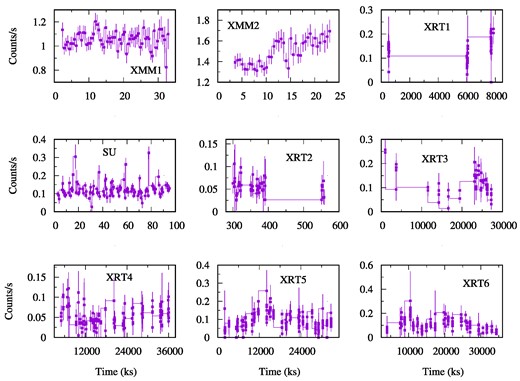
Variation of photon counts with respect to time from XMM–Newton, Suzaku and Swift/XRT observations of Mrk 6 at different epochs (see Table 1). The light curves in the 0.5–10.0 keV range are shown here.
3.1.1 Fractional variability
To check the temporal variability of Mrk 6 across different energy bands, we calculate the fractional variability Fvar (Edelson et al. 1996; Nandra et al. 1997; Rodríguez-Pascual et al. 1997; Vaughan et al. 2003; Edelson & Malkan 2012). The fractional variability for a light curve of xi counts/s with the measurement error σi for N number of data points, mean count rate μ and standard deviation σ, is given by the relation,
where, |$\sigma ^2_{\rm XS}$| is the excess variance (Nandra et al. 1997; Edelson et al. 2002), used to estimate the intrinsic source variance and given by,
Normalized excess variance is defined as |$\sigma ^2_{\rm NXS}=\sigma ^2_{\rm XS}/\mu ^2$|. The uncertainties in |$\sigma ^2_{\rm NXS}$| and Fvar are estimated as described in Vaughan et al. (2003) and Edelson & Malkan (2012). The peak-to-peak amplitude is defined as R = xmax/xmin (where, xmax and xmin are the maximum and minimum count rates, respectively) to investigate the variability in the X-ray light curves.
For both the XMM–Newton observations of Mrk 6 (XMM1 & XMM2), the results of the variability analysis for different energy bands are given in Table 2. During the XMM1 observation, we find that the peak-to-peak amplitude R varies in the range of 5.00 to 1.46. However, due to the low count rate and large error associated with each data point, we encounter negative values for |$\sigma ^2_{\rm NXS}$|, resulting in imaginary fractional variability (Fvar) for light curves in hard X-ray band and entire energy band. In the soft X-ray band, |$\sigma ^2_{\rm NXS}$| and Fvar are estimated to be 0.021 ± 0.020 and 14 per cent, respectively. Similarly, during the XMM2 observation, we find that R varies in the range of 1.54 to 1.29. However, |$\sigma ^2_{\rm NXS}$|, and Fvar are approximately the same for the soft, hard, and the entire energy bands with values of 0.003 ± 0.002 and ∼5.6 per cent, respectively. For NuSTAR observations (NU1 & NU2), the results of the variability analysis (xmax, xmin, μ) are presented in Table 2. The variation of the X-ray photons with time in band1 and band2 for both the observations (NU1 & NU2) are shown in the top middle panels of Fig. 2.
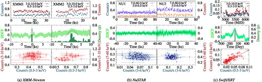
The multiplots display the light curves in different energy ranges, the correlation between the light curves, and the count–count plot from three different X-ray instruments (XMM–Newton, NuSTAR, and Swift/XRT). Top left-hand panels: The light curves of Mrk 6 in 0.5 to 3.0 keV (blue) and 3.0 to 10.0 keV (brown) ranges are presented for two epochs of XMM–Newton (XMM1 and XMM2) observations. The top middle panels show the light curves of the source in 3.0 to 6.0 keV (blue) and 7.0 to 60 keV (brown) ranges for two epochs of NuSTAR (NU1 and NU2) observations. The top right-hand panel shows the light curves of the source in 0.5 to 3.0 keV (blue) and 3.0 to 10 keV (brown) ranges for all the Swift/XRT observations of Mrk 6 between 2019 and 2022. It can be seen that the average count rate of the source in the high energy bands is high in comparison to the low energy band for all the observations. Middle panels: Corresponding ZDCF (light green) analysis curves showing the correlation as a function of time delay between the X-ray light curves are plotted. The likelihood functions (dark green), simulated using 102 000 points, are plotted along with the ZDCF. Lower panels: The count versus count plots are presented for all the observations.
The table provides variability statistics in different energy ranges for various observations, calculated using light curves with 500 s time bin. It is important to mention that in most of the cases, the average error of the observational data surpasses the 1σ limit, resulting in negative excess variance. As a result, these cases contain imaginary values for Fvar, and thus, they are excluded from the table.
| ID | Energy band | N | xmax | xmin | μ | |$R=\frac{x_{\rm max}}{x_{\rm min}}$| | |$\sigma ^{2}_{\rm NXS}$| | Fvar |
|---|---|---|---|---|---|---|---|---|
| keV | count s−1 | count s−1 | count s−1 | % | ||||
| XMM1 | 0.5–3.0 | 64 | 1.640 | 0.327 | 0.450 | 5.00 | 0.021 ± 0.020 | 14.0 ± 7.1 |
| 3.0–10.0 | 64 | 1.142 | 0.452 | 0.633 | 2.52 | −0.010 | – | |
| 0.5–10.0 | 63 | 1.204 | 0.824 | 1.053 | 1.46 | −0.002 | – | |
| XMM2 | 0.5–3.0 | 40 | 0.757 | 0.491 | 0.619 | 1.54 | 0.003 ± 0.002 | 5.6 ± 2.0 |
| 3.0–10.0 | 40 | 1.036 | 0.740 | 0.871 | 1.39 | 0.003 ± 0.016 | 5.3 ± 1.6 | |
| 0.5-10.0 | 40 | 1.694 | 1.311 | 1.490 | 1.29 | 0.003 ± 0.001 | 5.8 ± 1.2 | |
| NU1 | 3.0–6.0 | 151 | 0.103 | 0.017 | 0.065 | 6.50 | −0.006 | – |
| 7.0–60.0 | 156 | 0.603 | 0.147 | 0.261 | 4.10 | −0.004 | – | |
| 3.0–60.0 | 157 | 0.643 | 0.246 | 0.361 | 2.45 | −0.008 | – | |
| NU2 | 3.0–6.0 | 110 | 0.296 | 0.076 | 0.134 | 3.86 | −0.003 | – |
| 7.0–60.0 | 111 | 0.920 | 0.218 | 0.405 | 4.21 | 0.008 ± 0.004 | 9.3 ± 0.2 | |
| 3.0–60.0 | 112 | 5.244 | 0.437 | 0.635 | 12.00 | −0.054 | – | |
| XRT1 | 0.5–3.0 | 52 | 0.089 | 0.007 | 0.047 | 12.00 | 0.053 ± 0.040 | 23.0 ± 9.0 |
| 3.0–10.0 | 53 | 0.154 | 0.014 | 0.086 | 11.00 | 0.049 ± 0.026 | 22.0 ± 6.3 | |
| 0.5–10.0 | 53 | 0.221 | 0.032 | 0.132 | 6.87 | 0.037 ± 0.020 | 19.0 ± 5.7 | |
| XRT2 | 0.5–3.0 | 40 | 0.041 | 0.002 | 0.010 | 18.28 | −0.107 | – |
| 3.0–10.0 | 48 | 0.091 | 0.013 | 0.047 | 6.63 | −0.016 | – | |
| 0.5–10.0 | 47 | 0.106 | 0.025 | 0.055 | 4.08 | −0.008 | – | |
| XRT3 | 0.5–3.0 | 52 | 0.114 | 0.002 | 0.050 | 49.28 | 0.168 ± 0.046 | 4.1 ± 6.9 |
| 3.0–10.0 | 54 | 0.152 | 0.014 | 0.067 | 10.35 | 0.087 ± 0.031 | 29.0 ± 5.9 | |
| 0.5–10.0 | 53 | 0.257 | 0.031 | 0.117 | 8.08 | 0.101 ± 0.026 | 31.0 ± 5.0 | |
| XRT4 | 0.5–3.0 | 130 | 0.071 | 0.002 | 0.023 | 33.26 | −0.006 | – |
| 3.0–10.0 | 128 | 0.083 | 0.005 | 0.031 | 15.72 | 0.075 ± 0.030 | 27.0 ± 5.7 | |
| 0.5–10.0 | 125 | 0.122 | 0.015 | 0.055 | 7.78 | 0.022 ± 0.020 | 15.0 ± 6.9 | |
| XRT5 | 0.5–3.0 | 179 | 0.099 | 0.004 | 0.034 | 20.39 | 0.017 ± 0.022 | 13.0 ± 8.7 |
| 3.0–10.0 | 185 | 0.180 | 0.012 | 0.061 | 14.36 | 0.117 ± 0.021 | 34.0 ± 3.6 | |
| 0.5–10.0 | 185 | 0.257 | 0.020 | 0.093 | 12.40 | 0.080 ± 0.016 | 28.0 ± 3.3 | |
| XRT6 | 0.5–3.0 | 156 | 0.202 | 0.004 | 0.046 | 42.27 | 0.051 ± 0.034 | 22.0 ± 7.7 |
| 3.0–10.0 | 159 | 0.151 | 0.009 | 0.064 | 16.47 | 0.082 ± 0.023 | 28.0 ± 4.3 | |
| 0.5–10.0 | 161 | 0.303 | 0.030 | 0.107 | 10.01 | 0.073 ± 0.020 | 27.0 ± 4.1 | |
| XRT† | 0.5–3.0 | 511 | 0.098 | 0.001 | 0.011 | 55.04 | −0.209 | – |
| 3.0–10.0 | 637 | 0.293 | 0.008 | 0.083 | 35.80 | 0.196 ± 0.013 | 44.0 ± 1.9 | |
| 0.5–10.0 | 626 | 0.391 | 0.021 | 0.093 | 18.07 | 0.146 ± 0.012 | 38.3 ± 2.0 |
Note.† Represent combined Swift/XRT observation from XRT1(MJD-53754)-XRT6(MJD-59886).
For Swift/XRT observations, the variability parameters like |$\sigma ^2_{\rm NXS}$| and corresponding (Fvar) are also calculated. However, due to the low count rate and high error associated with each data point, we encounter negative values for normalized excess variance, resulting in imaginary fractional variability for the XRT2 observation. For observations with positive |$\sigma ^2_{\rm NXS}$|, the observed Fvar is found to be ranging from 4.1 to 23 per cent with an average of 16 per cent for the soft X-ray band. However, we find negative normalized excess variance for XRT4 in this energy band. In the hard X-ray band, Fvar is found to be 22 to 34 per cent with an average of 28 per cent. For the entire energy band, we obtain Fvar ranging from 15 to 31 per cent with a mean of 24 per cent. We also calculate the variability parameters of the combined Swift/XRT observations (XRT1–XRT6). In this case, we obtain Fvar as 44 per cent for the hard X-ray band and 38 per cent for the entire energy band. However, the average count rate in the soft X-ray band is very low (0.001 count s−1), causing noise dominance and resulting in negative normalized excess variance. The details of variability analysis are presented in Table 2.
Temporal variability in different energy bands provides insight into the physical properties of the emitting region. In the case of Mrk 6, the normalized excess variances were close to zero in the XMM–Newton (XMM1–MJD 51995) and NuSTAR (NU1 & NU2) observations, indicating the uncertainties of observed data surpassing the data dispersion. This implies insignificant variability above the count rate uncertainties, except for XMM2 (MJD–53670), which exhibited only |${\sim}5.7\pm 1.5\ \hbox{per cent}$|. In the combined Swift/XRT observations, over 20 per cent variability was detected. So, we can conclude that Mrk 6 shows temporal variability below 10 per cent in shorter time-scales (∼60 ks), whereas, for a longer time-scale (∼weeks), we observe over 20 per cent temporal variability.
3.1.2 Correlation
To investigate the correlation between the light curves, we conduct a detailed cross-correlation analysis of short-term and long-term X-ray observations of Mrk 6. We use two epochs of XMM–Newton (XMM1 & XMM2) and NuSTAR (NU1 & NU2) observations for the short-term study, whereas we employ the combined Swift/XRT observations (XRT3–XRT6) for the long-term analysis.
We use the ζ-transformed discrete correlation function (ζ−DCF9, Alexander 1997) method to investigate the correlation between the variation of photon counts in different energy bands. To determine the significance of the correlation function, we utilize the likelihood function for each discrete correlation function (DCF). For this purpose, we use 102 000 simulated points in the ζ−DCF code for the light curves obtained from the XMM–Newton, NuSTAR, and Swift/XRT observations. The error in the position of the peaks is calculated using the formula given in Gaskell & Peterson (1987), and the corresponding values are given in Table 3. The light curves with different energy bands from XMM–Newton, NuSTAR, and combined Swift/XRT observations are shown in the left-hand, middle, and right-hand top panels of Fig. 2, respectively. Furthermore, we plot the correlation function with corresponding light curves in the middle panels of Fig. 2. The count–count plots are also presented in the bottom panels of the same figure.
Details of the parameters utilized for estimating time delays between light curves in two different energy ranges. The peak value of the correlation function is denoted by |$\epsilon ^{z}_{\tau }$|, and the corresponding time delay is represented by |$\tau^{zdcf}_{\rm d}$|. Using the method outlined in (Gaskell & Peterson 1987), the error on the position of the peak of the correlation function is determined and is given by Δτd. A comparison between this error and the time bin size was conducted to ensure the accuracy of the result, with the larger value selected for our analysis. For further details, refer to Section 3.1.2.
| ID | Epochs | Bin size | Δτd | |$\epsilon ^{z}_{\tau }$| | |$\tau ^{zdcf}_{\rm d}$| |
|---|---|---|---|---|---|
| Year | (ks) | (ks) | (ks) | ||
| XMM1 | 2001 | 0.5 | 0.21 | 0.48 ± 0.05 | 0.31 ± 0.5 |
| XMM2 | 2005 | 0.5 | 0.46 | 0.50 ± 0.03 | 0.77 ± 0.5 |
| NU1 | 2015 | 0.5 | – | – | – |
| NU2 | 2015 | 0.5 | – | – | – |
| XRT† | 2019–2022 | 1.0 | 5.07 | 0.68 ± 0.05 | −1.88 ± 5.07 |
Note.† In the case of XRT observation, the correlation parameters are calculated in the unit of days.
We begin our analysis using the 2001 XMM–Newton observation (XMM1, MJD–51995). We find that the bin size of the light curve is larger than the value of uncertainty calculated using the formula given by Gaskell & Peterson (1987). So, we consider the bin size as the uncertainty on the position of the peak. We use a similar approach to estimate the delay in the light curves for the XMM2 observation. The estimated values are presented in Table 3.
In the case of NuSTAR observations, it is found that these two bands (band1 & band2) are uncorrelated. From the spectral analysis of these observations, we notice that below 10.0 keV, the X-ray photons originate from the Compton cloud, while above 10.0 keV, the reflection component dominates (see Section 3.2). We do not find any correlation between band1 and band2 as we examine the correlation between two types of photons with distinct origins.
We then proceed to investigate the light curves from Swift/XRT observations. Due to the limited resolution and low exposure time, we opt for a one-day bin size for the light curves from all XRT observations. The high uncertainty associated with smaller bin sizes, such as 500 s, led to the exclusion of many data points. We attempted different bin sizes for the light curves and found that the one-day bin is the optimum size for the temporal analysis. We consider 2019 to 2022 Swift/XRT observations, representing nearly continuous observations for our analysis. We exclude XRT1 (2006) and XRT2 (2015) observations due to their significant temporal separation from the nearly continuous XRT observations during 2019–2022. The light curves for two different bands are shown in the top right-hand panel of Fig. 2. We use similar techniques to calculate the correlation function (ζ−DCF). However, our analysis did not reveal any plausible time delay (−1.88 ± 5.07 d) between the soft X-ray and hard X-ray bands. The correlation function has a peak value of |$\epsilon ^{z}_{\tau }=0.68\pm 0.05$|. The detection of correlation between soft X-ray (0.5–3.0 keV) and hard X-ray (3.0–10.0 keV) bands suggests that the photons in both energy bands could have originated through the same physical mechanism (Kumari et al. 2021; Nandi et al. 2021, 2023). On the other hand, we find that the Swift/XRT spectra from 2019–2022 observations are well fitted by a single absorption coefficient (see Section 3.2). This finding indicates that the low-energy photons (below 3.0 keV) are less affected by column densities compared to other observations, where two absorption coefficients are required to fit the low-energy portions of each spectrum.
From the above study, it is evident that the light curves of soft X-ray and hard X-ray bands do not exhibit any significant correlation, or at most show very weak correlation during the XMM–Newton observations in 2001 (XMM1) and 2005 (XMM2). These observations are further characterized by the need for two absorption coefficients to fit the spectra below 3.0 keV, indicating a complex structure in the low-energy spectrum.
However, during the 2019–2022 Swift/XRT observations, a reasonably strong correlation is observed between these energy bands. From the spectral study of data from these observations, we find that the low-energy part of the X-ray spectrum is relatively simple for Swift/XRT observations. It is well fitted with a single absorption coefficient model. In the case of a high energy band (above 10.0 keV), we observe the domination of the reflection component over the primary continuum. As a result, the light curves in band1 and band2 are found to be uncorrelated. The detailed results are given in Table 3, and the corresponding correlation functions are plotted in the middle panels of Fig. 2.
3.2 Spectral analysis
We use data from XMM–Newton, NuSTAR, Suzaku, and Swift/XRT observations of Mrk 6 in our spectral analysis to investigate the spectral variations of the source over an extensive time frame of ∼22 years (2001–2022). We use |$\tt {XSPEC}$| v12.12.1 (Arnaud 1996) software package for spectral analysis. The χ2 statistics is used to determine the best-fitting models to describe the observed data. The spectral analysis is carried out using XMM–Newton observations in 2001 and 2005 in the 0.5–10 keV range, simultaneous Suzaku and NuSTAR observations in the 0.5–60 keV range, simultaneous Swift/XRT and NuSTAR observations in the 0.5–60 keV range, and XRT observations for 13 epochs from 2006 to 2022 in the 0.5–10 keV range (see Table 1). NuSTAR data beyond 60 keV are not considered in the present analysis as it is dominated by background. To ensure robust statistics, we bin the data in such a way that there are at least 30 counts/bin for both XMM–Newton, Suzaku, and NuSTAR observations, while we used 10 counts in each bin for the Swift/XRT observations. The GRPPHA task is used for binning the spectral data. The quoted errors for best-fitting spectral parameters are determined at a 90 per cent confidence level by using the command error in Xspec. We calculate the unabsorbed X-ray luminosity from each spectrum using clumin10 on the powerlaw model. We estimate the Eddington luminosity LEdd = 1.95 × 1046 erg s−1 by using the relation, LEdd = 1.3 × 1038(MBH/M⊙), where MBH = 1.5 × 10⁸ M⊙ (Afanasiev et al. 2014). The bolometric luminosity is calculated using the intrinsic luminosity of the source in the energy range from 2.0 to 10.0 keV with the bolometric correction factor 20 (Vasudevan & Fabian 2009). While estimating the luminosity, we use the redshift, z = 0.0186. Using the bolometric luminosity and Eddington luminosity of the source, we derive the Eddington ratio (λEdd), which is defined as the ratio between the bolometric luminosity (Lbol) and Eddington luminosity (LEdd). Throughout this work, we use the Cosmological parameters as follows: |${H}_0 = 70 \, \text{km s}^{-1} \, \text{Mpc}^{-1}, \Lambda _0 = 0.73, {\rm and}\ \sigma _{\rm M} = 0.27$| (Bennett et al. 2003).
3.2.1 Model construction
To investigate the spectral variability in the source during our observation period, we construct a base model covering the broad energy range from 0.5 to 60.0 keV. We begin by employing simple models, such as the power law, to characterize the observed X-ray spectra. Later, these models are replaced with more sophisticated phenomenological and physical models to understand the accretion dynamics and other physical properties. A constant component is used as a cross-normalization factor while using data from different instruments in simultaneous (SU+NU1 and XRT2+NU2) spectral fitting.
Initially, we consider the 3.0 to 10.0 keV X-ray continuum spectrum of the source for spectral fitting. According to current understanding, the X-ray continuum photons are produced through the process of inverse Compton scattering, wherein the thermal photons from the accretion disc are up-scattered in a hot electron cloud. This process can produce a power-law type of spectrum. Therefore, we consider powerlaw model to fit the spectrum of each observation given in Table 1. Along with this, we also consider Galactic hydrogen column density (NH, gal) along the line of sight as the multiplicative model TBabs (Wilms, Allen & McCray 2000) within XSPEC. We fix the value of NH, gal at 7.63 × 1020 cm−2, the Galactic value in the direction of the source.11 Thus, our base model for the 3.0 to 10.0 keV X-ray spectral fitting is as follows:
|${\tt TBabs \times const \times powerlaw}.$|
We fit each spectrum with this model, and the corresponding variation of χred for XRT2+NU2 (MJD–57335) observation is illustrated in the panel (a) of Fig. 3. After the continuum fitting, we observe positive residuals in the 6–7 keV range (see Fig. 3(a)), which is attributed to the presence of Fe Kα line. To account for this, we introduced a Gaussian model, zGauss in Xspec. As a result, our model to fit the spectrum in the 3.0 to 10.0 keV range is as follows:
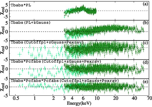
Variation of χred values is shown for each model across the broad-band (XRT2+NU2) spectra of Mrk 6. The analysis started in the 3.0–10.0 keV range spectrum with the simple powerlaw model, and corresponding residuals are shown in the top panel (a). Then, we added zGaussian for the Fe-line at ∼6.45 keV. Later, we extended spectra above 10 keV. The corresponding residuals are shown in the second panel (b). The pexrav model was used to account for the reflection component. Next, we extended the spectra below 3.0 keV, and the corresponding residuals are shown in the third panel (c). The residuals obtained by adding single and double pcfabs components to account for the absorption characteristics of the local absorber in the soft X-ray ranges are shown in the fourth (d) and fifth (e) panels, respectively.
|${\tt TBabs \tt \times const(powerlaw+zGauss)}.$|
After successfully fitting the primary continuum and the iron Kα line in 3.0 to 10.0 keV range (see Fig. 3(b)), we proceed to extend the X-ray spectra into the high energy regime (above 10 keV). In doing this, we find that the observational broad-band data do not align with our model (Fig. 3(b)). We use another powerlaw to address this deviation in the high-energy data points from the primary model. Subsequently, this additional power-law component is later substituted with pexrav, and the corresponding variation of χred is shown in Fig. 3(c). It is to be noted that the powerlaw component is replaced by a cut-off power law (cutoffpl) to investigate the presence of a high-energy cut-off in the broad-band observations. So, for broad-band observations, the model became:
|${\tt TBabs\times const(cutoffpl+zGauss+pexrav)}.$|
To address the low-energy counterpart of the observed X-ray spectra (below 3.0 keV), we initially employ a single pcfabs12 along with the |${\tt TBabs \times const(cutoffpl+zGauss+pexrav)}$| model. The corresponding variation of χred is shown in Fig. 3(d) for the observation XRT2+NU2. It is evident in this panel that a single pcfabs is insufficient to account for the local hydrogen column density along the line of sight. Therefore, we introduce another pcfabs to fit the broad-band spectrum in the 0.5–60.0 keV range, and the corresponding variation of χred is shown in Fig. 3(e). As a result, the composite model employed to fit the broad-band spectra can now be defined as follows:
|$\tt { TBabs\times pcfabs\times pcfabs\times const(cutoffpl+zGauss} \\{+pexrav)}.$|
To investigate the ionization properties of the absorber, we replace the second pcfabs component with zxipcf (Miller et al. 2006; Reeves et al. 2008) component. It is worth mentioning that a previous study by Feldmeier et al. (1999), Immler et al. (2003), and Malizia et al. (2003) also employed double absorption components and suggested that one absorber might be located in proximity to the black hole or within the BLR region, while the second absorber could be situated further away, possibly within the torus. This model (zxipcf) can calculate the amount of ionization of the medium through the ionization parameter |$\rm (\xi)$| as |$\xi =L/(nR^2)$|, where L is the luminosity of the irradiating source, n is the number density of the irradiated material, and R is the distance between the source and the irradiated material.
It is noted that while fitting data in the 0.5–10 keV range (XMMs and XRT observations in Table 1), we use |${\tt TBabs \times pcfabs \times pcfabs \times (powerlaw+zGauss)}$| and |${\tt TBabs\times pcfabs \times zxipcf \times (powerlaw+zGauss)}$| as our composite models.
3.2.2 powerlaw
We started our spectral analysis with an absorbed power-law model with a Gaussian line (zGauss) as described in Section 3.2.1. The model in Xspec reads as: |${\tt TBabs\!\times \! pcfabs\!\times \!pcfabs\!\times \! (powerlaw + zGauss)}$|. This composite model fits the X-ray spectra up to 10.0 keV. Corresponding power-law indices are found to be Γ = 1.53 ± 0.10 and 1.57 ± 0.10 for XMM1 and XMM2 observations, respectively. Next, we analyse the data obtained from the Swift/XRT observations of the source for the energy range of 0.5–10 keV. Across all 13 XRT spectra, the Fe Kα line remains undetected. This could be due to the low exposure time of each observation, combined with the poor energy resolution of Swift/XRT. Therefore, we fit the Swift/XRT spectra by removing the Gaussian component from the baseline model. The resultant fitted model in Xspec reads as: |${\tt TBabs \times pcfabs \times pcfabs \times powerlaw}$|. From the analysis of XRT1 (MJD–53754), we find that the column densities increased and photon index (Γ) changed from, Γ ∼1.57 to 1.73 after the XMM2 observation (MJD–53670).
In the subsequent analysis, we use the data from two broad-band observations, namely, SU+NU1 (MJD–57133) and XRT2+NU2 (MJD–57335), in the energy range of 0.5–60 keV. The parameters obtained after applying the best-fitted composite model to the spectra are Γ = 1.72 ± 0.05 and 1.73 ± 0.02, iron Kα line at 6.39 ± 0.06 and 6.25 ± 0.10 keV with EW of |$156^{+98}_{-75}$| and |$103^{+30}_{-30}$|, respectively. The broad-band spectra fitted with this composite model for the SU+NU1 and XRT2+NU2 observations are shown in Fig. 5. Next, we replaced the second pcfabs component with zxipcf to check the ionization of the absorber. The best-fitting values obtained in the presence of an ionized absorber are reported in Table 4.
Best-fitting parameters obtained from the spectral fitting of the data with Model: |${\tt TBabs\times pcfabs\times zxipcf\times (powerlaw+zGauss)}$|. The ionizing luminosity |$L_{\rm ion}$| is calculated in the energy range of 13.6 eV–13.6 keV (1–1000 Ryd).
| Id | MJD | NH i | Cf1 | NH2 | |$\log\xi$| | Cf2 | Γ | NormPL | |$\chi ^{2}/\rm dof$| | log Lion | rmax |
|---|---|---|---|---|---|---|---|---|---|---|---|
| (1022 cm−2) | (1022 cm−2) | (10−3) | |$\log ({\rm erg\,s}^{-1})$| | pc | |||||||
| photons keV−1 cm−2 s−1 | |||||||||||
| XMM1 | 51 995 | |$1.31^{+0.57}_{-0.38}$| | |$0.91^{+0.05}_{-0.06}$| | |$6.47^{+2.65}_{-1.10}$| | |$1.08^{+0.23}_{-0.26}$| | |$0.70^{+0.14}_{-0.17}$| | |$1.58^{+0.08}_{-0.08}$| | |$3.48^{+0.27}_{-0.28}$| | 763.02/740 | |$43.51^{+0.03}_{-0.02}$| | 13.50 |
| XMM2 | 53 670 | |$1.76^{+0.21}_{-0.50}$| | |$0.93^{+0.05}_{-0.05}$| | |$5.83^{+1.07}_{-1.01}$| | |$1.20^{+0.20}_{-0.19}$| | |$0.67^{+0.17}_{-0.18}$| | |$1.56^{+0.10}_{-0.09}$| | |$5.55^{+1.30}_{-0.40}$| | 595.08/658 | |$43.65^{+0.06}_{-0.04}$| | 15.69 |
| XRT1 | 53 754 | |$1.95^{+1.01}_{-1.02}$| | |$0.85^{+0.05}_{-0.04}$| | |$6.69^{+4.52}_{-8.39}$| | |$1.05^{+0.15}_{-0.19}$| | |$0.80^{+0.04}_{-0.03}$| | |$1.71^{+0.10}_{-0.15}$| | |$4.95^{+0.27}_{-0.28}$| | 118.81/115 | |$43.58^{+0.02}_{-0.04}$| | 16.44 |
| SU+NU1 | 57 133 | |$2.76^{+0.52}_{-0.92}$| | |$0.71^{+0.04}_{-0.04}$| | |$12.91^{+3.40}_{-11.10}$| | |$1.03^{+0.16}_{-0.30}$| | |$0.81^{+0.01}_{-0.02}$| | |$1.72^{+0.10}_{-0.09}$| | |$3.00^{+0.10}_{-0.08}$| | 357.49/388** | |$43.25^{+0.03}_{-0.06}$| | 4.17 |
| XRT2+NU2 | 57 335 | |$7.70^{+1.03}_{-1.90}$| | |$0.88^{+0.02}_{-0.05}$| | |$12.65^{+7.75}_{-8.20}$| | |$1.10^{+0.44}_{-0.29}$| | |$0.92^{+0.02}_{-0.02}$| | |$1.73^{+0.07}_{-0.10}$| | |$4.86^{+0.87}_{-0.71}$| | 442.03/457** | |$43.37^{+0.03}_{-0.05}$| | 4.78 |
Note.** The fit statistics for each instrument in the broad-band fitting SU+NU1 is: 96.67/68 for XIS, 135.11/162 for FPMA, and 125.71/158 for FPMB. Similarly, in XRT2+NU2 broad-band fitting, fit statistics is: 104.67/123 for XRT, 188.73/166 for FPMA, and 148.63/168 for FPMB.
Applying the same baseline model to the remaining 12 Swift/XRT observations, we find that the double pcfabs does not significantly improve the fit. This could be due to the low exposure time of the observations, relatively poor energy resolution of XRT, or the absence of the second absorber. Consequently, we opt to substitute the double pcfabs with a single pcfabs from XRT3a (MJD–58647) to XRT6c (MJD–59886). In these cases, our chosen baseline model becomes |${\tt TBabs\times pcfabs \times powerlaw}$|. Across these observations, the average photon index (Γ) is estimated as 1.43. For the single absorber, the absorption column density and corresponding covering factor vary in the ranges of (|$2.48^{+0.46}_{-0.51}$|–|$5.34^{+1.75}_{-1.60})\times 10^{22}~\text{cm}^{-2}$|, and (|$0.90^{+0.06}_{-0.15}$|–|$0.97^{+0.01}_{-0.03})$|, respectively. The X-ray continuum luminosity of the source in the 3.0–10.0 keV energy band, estimated from the power-law fitting to the data from these observations, varies in the range of |$42.45^{+0.10}_{-0.10}$| to |$42.92^{+0.02}_{-0.02}$|, whereas the Eddington ratio |$\log(\lambda_{\rm Edd})$| varied in the range of −2.40 to −1.97. The details of the best-fitted results are given in Table 5.
Parameters obtained from the |${\tt TBabs\times pcfabs\times pcfabs\times (powerlaw+zGauss)}$| model fitting with all the spectra for the energy range of 0.5 to 10 keV. The unabsorbed X-ray continuum luminosity is calculated for the energy range of 3.0 to 10.0 keV. The detailed results are discussed in Section 3.2.2
| Id | MJD | NH i | Cf1 | NH2 | Cf2 | Γ | |${\rm Norm}^{\rm PL^\dagger }$| | Fe Kα | EW | |${\rm Norm}^{k_\alpha ^\dagger }$| | |$\log L_{x}$| | |$\log \lambda_{\rm Edd}$| | |$\chi ^{2}/\rm dof$| |
|---|---|---|---|---|---|---|---|---|---|---|---|---|---|
| (1022 cm−2) | (1022 cm−2) | (10−3) | (keV) | (eV) | (10−5) | |$\log({\rm erg\,s}^{-1})$| | |||||||
| XMM1 | 51995 | |$1.97^{+0.26}_{-0.30}$| | |$0.92^{+0.01}_{-0.03}$| | |$6.21^{+2.16}_{-1.72}$| | |$0.54^{+0.09}_{-0.09}$| | |$1.53^{+0.10}_{-0.08}$| | |$3.34^{+0.73}_{-0.57}$| | |$6.43^{+0.04}_{-0.05}$| | |$128^{+28}_{-26}$| | |$2.64^{+1.08}_{-0.83}$| | |$43.06^{+0.03}_{-0.03}$| | |$-1.83^{+0.02}_{-0.02}$| | 764.06/741 |
| XMM2 | 53670 | |$1.92^{+0.25}_{-0.37}$| | |$0.94^{+0.01}_{-0.03}$| | |${ 5.26^{+2.20}_{-1.82}}$| | |$0.51^{+0.13}_{-0.11}$| | |$1.57^{+0.10}_{-0.10}$| | |$5.00^{+1.08}_{-0.86}$| | |$6.40^{+0.04}_{-0.03}$| | |$61^{+22.70}_{-23.20}$| | |$1.75^{+0.64}_{-0.65}$| | |$43.17^{+0.03}_{-0.04}$| | |$-1.70^{+0.02}_{-0.02}$| | 590.27/660 |
| XRT1 | 53754 | |$3.21^{+0.61}_{-1.28}$| | |$0.95^{+0.02}_{-0.07}$| | |$27.32^{+2.72}_{-2.14}$| | |$0.62^{+0.03}_{-0.03}$| | |$1.73^{+0.10}_{-0.15}$| | |$6.94^{+2.3}_{-1.5}$| | – | – | – | |$42.81^{+0.06}_{-0.05}$| | |$-2.05^{+0.05}_{-0.05}$| | 119.97/116 |
| SU+NU1 | 57 133 | |$4.97^{+3.38}_{-1.77}$| | |$0.78^{+0.03}_{-0.03}$| | |$30.68^{+4.29}_{-3.37}$| | |$0.77^{+0.09}_{-0.03}$| | |$1.72^{+0.06}_{-0.04}$| | |$3.22^{+0.19}_{-0.17}$| | |$6.39^{+0.06}_{-0.06}$| | |$156^{+98}_{-75}$| | |${1.78^{+0.37}_{-0.36}}$| | |$42.88^{+0.02}_{-0.02}$| | |$-2.08^{+0.01}_{-0.01}$| | 364.51/389** |
| XRT2+NU2 | 57335 | |$5.18^{+0.98}_{-0.89}$| | |$0.78^{+0.05}_{-0.04}$| | |$14.24^{+1.22}_{-1.27}$| | |$0.87^{+0.02}_{-0.02}$| | |$1.73^{+0.02}_{-0.02}$| | |$2.98^{+0.02}_{-0.02}$| | |$6.25^{+0.12}_{-0.09}$| | |$103^{+30}_{-30}$| | |$1.29^{+0.41}_{-0.49}$| | |$43.03^{+0.05}_{-0.05}$| | |$-1.87^{+0.02}_{-0.02}$| | 445.34/458** |
| XRT3a | 58 647 | |$3.98^{+1.33}_{ -0.95}$| | |$0.92^{+0.02}_{ -0.02}$| | – | – | |$1.37^{+0.12}_{ -0.10}$| | |$1.72^{+0.2}_{-0.2}$| | – | – | – | |$42.86^{+0.04}_{ -0.06}$| | |$-2.01^{+0.05}_{-0.05}$| | 62.97/49 |
| XRT3b | 58 806 | |$2.72^{+0.74}_{ -0.80}$| | |$0.97^{+0.01}_{- 0.03}$| | – | – | |$1.44^{+0.16}_{-0.15}$| | |$3.06^{+1.20}_{-1.46}$| | – | – | – | |$42.89^{+0.08}_{ -0.08}$| | |$-1.98^{+0.08}_{-0.08}$| | 39/50 |
| XRT3c | 58 832 | |$2.86^{+1.14}_{ -1.09}$| | |$0.91^{+0.05}_{ -0.12}$| | – | – | |$1.41^{ +0.16}_{ -0.17}$| | |$1.10^{+0.13}_{-0.61}$| | – | – | – | |$42.79^{+0.03}_ {- 0.04}$| | |$-2.12^{+0.04}_{-0.04}$| | 54.48/45 |
| XRT4a | 58 892 | |$4.07^{ + 1.47 }_{ - 1.46}$| | |$0.90^{ + 0.06}_{- 0.15}$| | – | – | |$1.41^{+ 0.07}_{ - 0.06}$| | |$0.84^{+0.11}_{-0.52}$| | – | – | – | |$42.54^{ + 0.06}_{- 0.06}$| | |$-2.34^{+0.06}_{-0.06}$| | 59.63/45 |
| XRT4b | 59 004 | |$5.34^{ + 1.75 }_{ - 1.60}$| | |$0.91^{ + 0.04}_{- 0.10}$| | – | – | |$1.58^{+ 0.17}_{ - 0.15}$| | |$0.91^{+0.88}_{-0.56}$| | – | – | – | |$42.45^{ + 0.10}_{- 0.10}$| | |$-2.40^{+0.10}_{-0.10}$| | 32.95/36 |
| XRT4c | 59 135 | |$4.03^{ + 1.19 }_{ - 1.12}$| | |$0.93^{ + 0.03}_{- 0.07}$| | – | – | |$1.39^{+ 0.13}_{ - 0.11}$| | |$1.00^{+0.75}_{-0.50}$| | – | – | – | |$42.63^{ + 0.07}_{- 0.06}$| | |$-2.26^{+0.07}_{-0.07}$| | 57.60/64 |
| XRT5a | 59 271 | |$4.60^{ + 0.98 }_{ - 0.98}$| | |$0.94^{ + 0.02 }_{ - 0.03}$| | – | – | |$1.41^{+ 0.18}_{ - 0.23}$| | |$1.29^{+0.47}_{-0.51}$| | – | – | – | |$42.76^{+ 0.03}_{- 0.03}$| | |$-2.14^{+0.03}_{-0.03}$| | 82.27/94 |
| XRT5b | 59 388 | |$3.68^{ + 0.60 }_{ - 0.60}$| | |$0.96^{ + 0.01 }_{ - 0.02}$| | – | – | |$1.40^{+ 0.24}_{ - 0.23}$| | |$1.96^{+1.00}_{-0.62}$| | – | – | – | |$42.92^{+ 0.02}_{- 0.02}$| | |$-1.97^{+0.02}_{-0.02}$| | 148.68/143 |
| XRT5c | 59 523 | |$3.45^{ + 0.68 }_{ - 0.64}$| | |$0.94^{ + 0.02 }_{ - 0.03}$| | – | – | |$1.41^{+ 0.21}_{ - 0.23}$| | |$1.21^{+0.50}_{-0.43}$| | – | – | – | |$42.77^{+ 0.02}_{- 0.02}$| | |$-2.13^{+0.03}_{-0.03}$| | 111.02/135 |
| XRT6a | 59 641 | |$3.12^{ + 0.53 }_{ - 0.57}$| | |$0.97^{ + 0.01 }_{ - 0.02}$| | – | – | |$1.43^{+ 0.20}_{ - 0.14}$| | |$2.09^{+0.80}_{-0.30}$| | – | – | – | |$42.92^{+ 0.06}_{- 0.05}$| | |$-1.97^{+0.03}_{-0.03}$| | 125.27/132 |
| XRT6b | 59 752 | |$2.48^{ + 0.46 }_{ - 0.51}$| | |$0.96^{ + 0.01 }_{ - 0.01}$| | – | – | |$1.41^{+ 0.22}_{ - 0.23}$| | |$1.52^{+0.67}_{-0.46}$| | – | – | – | |$42.81^{+ 0.03}_{- 0.03}$| | |$-2.07^{+0.03}_{-0.03}$| | 119.29/127 |
| XRT6c | 59 886 | |$3.24^{ + 0.62 }_{ - 0.62}$| | |$0.95^{ + 0.03 }_{ - 0.03}$| | – | – | |$1.49^{+ 0.20}_{ - 0.26}$| | |$1.66^{+0.57}_{-0.52}$| | – | – | – | |$42.73^{+ 0.04}_{- 0.03}$| | |$-2.16^{+0.03}_{-0.03}$| | 99.05/115 |
Note.† In the unit of photons keV−1 cm−2 s−1 ** The fit statistics for each instrument in the broad-band fitting SU+NU1 is: 106.26/69 for XIS, 133.69/162 for FPMA, and 124.56/158 for FPMB. Similarly, in XRT2+NU2 broad-band fitting, fit statistics is: 104.48/124 for XRT, 191.71/166 for FPMA, and 149.15/168 for FPMB.
The luminosity variation in X-ray band (Lx), Eddington ratio (λEdd), photon index (Γ), hydrogen column densities for the two distinct absorbers (NH i & NH2), and corresponding covering factors (Cf1 & Cf2) are graphically presented in Fig. 4, for all the observations used in the present work. The X-ray luminosity of the source remains comparable throughout our observational period and is presented in panel (a) of Fig. 4. The average value of |$\log(L_x)$| is |$42.82^{+0.07}_{-0.07}$|, with the highest and lowest values being |$43.17^{+0.01}_{-0.01}$| and |$42.45^{-0.10}_{+0.10}$|, respectively. The Eddington ratio of Mrk 6 is shown in panel (b) of Fig. 4.
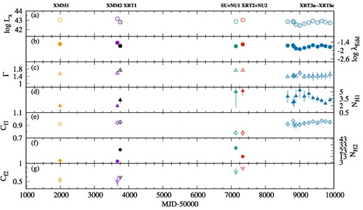
Temporal variations of X-ray luminosity (Lx), Eddington ratio (λEdd), photon index (Γ), hydrogen column density, and corresponding covering factor for two distinct absorbers (NH i & Cf1, and NH2 & Cf2) are shown for all the observations used in the present work. The values of Lx and λEdd are plotted in logarithmic scale. The values of the parameters are also given in Table 5.
However, we observe that the photon index (Γ) varies between |$1.37^{+0.12}_{-0.10}~\text{and}~ 1.73^{+0.02}_{-0.02}$|. The variation of Γ is presented in panel (c) of Fig. 4. We observe that Mrk 6 has a complex column density structure around it. In the initial phase of our observations, two-column densities of different natures are used to describe the absorption. However, towards the later part of our observation (from XRT3b), the complexity in the absorption disappears. The variation of hydrogen column density with the corresponding covering factor for both the absorbers are shown in panels (d, e) and (f, g) of Fig. 4, respectively. Fig. 5 shows the best-fitting spectrum obtained with the powerlaw model.
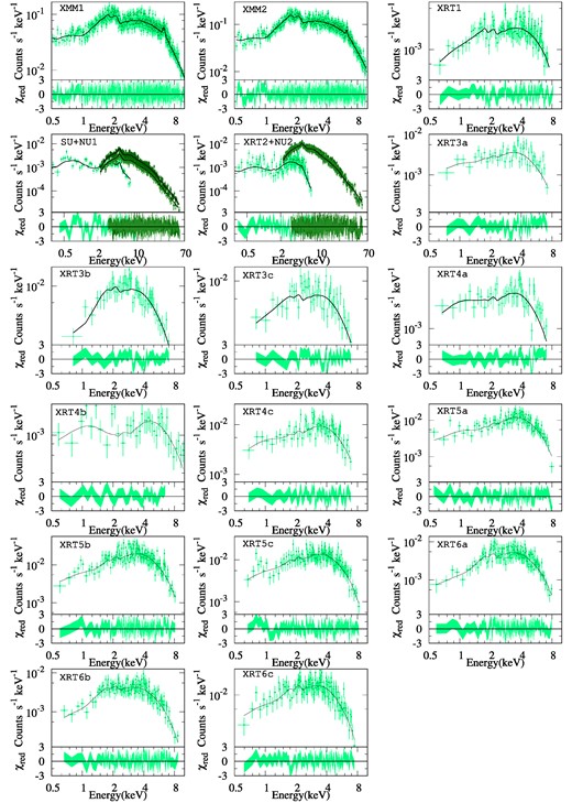
Powerlaw model fitted spectra of Mrk 6 from the XMM–Newton, Suzaku, NuSTAR, and Swift observations along with the residuals obtained from the spectral fitting.
3.2.3 nthcomp model
As the power-law model effectively fits the primary continuum in the 3.0–10.0 keV range, we attempt to estimate the temperature of the Compton cloud. Hence, we replace the powerlaw with nthcomp model (Zdziarski, Johnson & Magdziarz 1996; Życki, Done & Smith 1999). The thermally Comptonized continuum model is parametrized by the hot electron temperature kTe. This model depends on the energy of the seed photons (kTbb), which we consider at 10 eV for all the observations. It is to be noted that we vary this parameter from 1 to 50 eV and do not notice any variation in the residuals of the fitted spectra. Alongside this, we consider disc-blackbody type seed photons for this work. To do so, we opt int-type=1 for all the spectral fitting. The nthcomp model provides us the photon index (Γ) and the hot electron temperature of the Compton cloud (kTe). Furthermore, we calculate the optical depth (τ) for each observation using the formula:
by using the relation as presented in Zdziarski, Johnson & Magdziarz (1996), where |$\theta_{\rm e} = \frac{kT_{\rm e}}{m_{\rm e}c^{2}}$| is the electron energy with respect to the rest mass energy.
Simultaneous broad-band observations of Mrk 6 were carried out with Suzaku and NuSTAR, and Swift/XRT and NuSTAR, at two epochs, separated by 202 days. While fitting the broad-band spectra for both the epochs with the nthcomp model, we find that the photon index (Γ) remains almost constant (Γ ∼ 1.70–1.72). This suggests that the nature of the Compton cloud remained stable over this period. The electron cloud temperature (kTe) is found to exceed 65 keV for SU+NU1 observation and is determined as |$69^{+15}_{-9}$| keV for XRT2+NU2 observation. In both cases, the values of the optical depth (τ) remain almost constant (τ ∼ 1.83–1.71). The results obtained from our spectral fitting with this model are listed in Table 6. We also include a Gaussian component to account for the Fe-line near ∼6.4 keV, and the results closely resemble those obtained from the power-law fitting.
nthcomp model fitting results for the spectrum above 3.0 keV.
| Id | MJD | Γ | kTe | Normnth | |$\chi ^{2}/\rm dof^{**}$| | τ* |
|---|---|---|---|---|---|---|
| (keV) | (10−3) | |||||
| photons keV−1 cm−2 s−1 | ||||||
| SU+NU1 | 57 133 | |$1.70^{+0.09}_{-0.10}$| | >65 | |$3.52^{+0.31}_{-0.30}$| | 305.43/363 | <1.83 |
| XRT2+NU2 | 57 335 | |$1.72^{+0.05}_{-0.07}$| | |$69.51^{+14.82}_{-9.46}$| | |$2.98^{+0.36}_{-0.23}$| | 416.06/419 | |$1.71^{+0.23}_{-0.58}$| |
Note. ** The fit statistics for each instrument in the broad-band fitting SU+NU1 is: 48.04/45 for XIS, 132.88/161 for FPMA, and 124.51/157 for FPMB. Similarly, in XRT2+NU2 broad-band fitting, fit statistics is: 69.13/85 for XRT, 191.81/166 for FPMA, and 155.12/168 for FPMB. * The optical depth is not estimated from the spectral fitting. It is calculated using equation (3).
3.2.4 pexrav model
Although the power-law model provides a satisfactory fit of the primary continuum in the 3.0–10.0 keV energy range, these models fail to characterize the high energy (above 10.0 keV) counterpart of the observed spectrum of Mrk 6. So, we use another power law, which is found to be flattened compared to the continuum. Moreover, the Fe line EW of more than 200 eV is a signature of the presence of a reflection component from an obscured medium (Krolik, Madau & Zycki 1994). The flatness of the second power-law component, along with the high equivalent width of the observed Fe Kα line, suggests the presence of a reflection component in the broad-band spectrum of Mrk 6. To address the reflection component, we substitute the second power law with the slab reflection model pexrav (Zdziarski, Johnson & Magdziarz 1996). Consequently, the composite model utilized to fit the broad-band spectra of both the epochs of observations is as follows:
The two column densities, namely pcfabs and zxipcf, are used to incorporate absorption along the line of sight (for more details, see Section 3.2.2). Regarding the model pexrav, we tie the photon index with the cut-off power-law index (Γ) while keeping this Γ as a free parameter. As the cut-off power-law model is used as the primary continuum, we constrain relrefl < 0, indicating that pexrav solely contributes to the reflection component only. We fix the abundance to the solar value while the inclination angle (i) and reflection fraction (Rf) are kept free during spectral fitting.
For the SU+NU1 (MJD–57133) observation, we find the photon index and cut-off energy at |$\Gamma =1.72^{+0.10}_{-0.09}$| and |$E_{\rm c}=111^{+39}_{-28}$| keV, respectively. The pexrav component of the composite model gives the value of the reflection coefficient as |$R_{\rm f}=1.85^{+0.16}_{-0.15}$|. Subsequently, in the case of the XRT2+NU2 (MJD–57335) observation, we find |$\Gamma =1.75^{+0.07}_{-0.10}$|, cut-off energy |$E_{\rm c}=121^{+38}_{-35}$| keV, and reflection fraction |$R_{\rm f}=1.02^{+0.15}_{-0.18}$|. The comparable parameters obtained during the two epochs of observations may be due to the 202-day gap between the epochs, during which the source properties did not show any noticeable change in its properties. It is to be noted that the parameter i is insensible during these spectral fittings. We obtained that i = 63 ± 45° for both cases. The results obtained from our spectral fitting with this model are listed in Table 7 .
The parameters obtained from the spectral fitting of broad-band (0.5 to 60.0 keV) data of Mrk 6 with the model: |${\tt TBabs\times pcfabs\times zxipcf\times const(cutoffpl+zGauss+pexrav)}$|.
| Id | MJD | NH i | Cf1 | NH2 | Cf2 | |$\log \xi$| | Γ | EC | Rf | Norm | |$\chi ^{2}/\rm dof^{**}$| |
|---|---|---|---|---|---|---|---|---|---|---|---|
| (1022 cm−2) | (1022 cm−2) | (keV) | (10−3) | ||||||||
| photons keV−1 cm−2 s−1 | |||||||||||
| SU+NU1 | 57 133 | |$3.20^{+0.52}_{-0.57}$| | |$0.49^{+0.18}_{-0.19}$| | |$17.56^{+1.15}_{-2.45}$| | |$0.91^{+0.18}_{-0.14}$| | |$0.98^{+0.11}_{-0.51}$| | |$1.72^{+0.10}_{-0.09}$| | |$111^{+39}_{-28}$| | |$1.85^{+0.16}_{-0.15}$| | |$2.41^{+0.70}_{-0.47}$| | 751.16/814 |
| XRT2+NU2 | 57 335 | |$3.36^{+0.55}_{-0.64}$| | |$0.57^{+0.04}_{-0.04}$| | |$12.60^{+5.14}_{-5.41}$| | |$0.96^{+0.22}_{-0.29}$| | |$0.82^{+0.12}_{-0.15}$| | |$1.75^{+0.07}_{-0.10}$| | |$121^{+38}_{-35}$| | |$1.02^{+0.15}_{-0.18}$| | |$4.86^{+0.87}_{-0.71}$| | 889.50/881 |
Note.** The fit statistics for each instrument in the broad-band fitting SU+NU1 is: 102.97/71 for XIS, 338.32/381 for FPMA, and 309.87/362 for FPMB. Similarly, in XRT2+NU2 broad-band fitting, fit statistics is: 118.25/130 for XRT, 443.04/381 for FPMA, and 328.21/370 for FPMB.
3.2.5 Borus model
Although the disc-reflection model provides an acceptable fit, it is worth noting that the pexrav model is inadequate to explain the properties of the reflective medium in detail. Indeed, this reflection model offers valuable insights into the temperature of the Compton cloud and the reflection coefficient. However, it is important to highlight that pexrav assumes an infinite line-of-sight column density and overlooks the finite characteristics of the reflecting medium. Therefore, in the subsequent analysis, we opt for a more comprehensive toroidal reflection model known as borus13 (Baloković et al. 2018). This model assumes a spherical reprocessing medium with a conical cut-out at the poles. This provides a toroidal structure of the reflecting materials, exhibiting a variable covering factor. For this work, we use borus0214 model, which offers supplementary information on parameters such as the cut-off energy (Ecut) and abundance of Fe (AFe) in addition to other model parameters. The composite model employed to fit the broad-band spectra using borus02 is described as follows:
|${\tt zphabs\times cabs\times cutoffpl1}$| represents the absorbed direct primary emission while |${\tt const2\times cutoffpl2}$| represents the scattered primary emission. In the above model, const1 and const2 are instrument cross-normalization and the relative normalization of a leaked or scattered unabsorbed reflection of the intrinsic continuum, respectively. We allow the torus column density (|$N_{\rm H}^{\rm tor}$|) with the toroidal angle (θtor) and the inclination angle (i) to vary freely during the broad-band spectral fitting, as these parameters are unknown to us. For other model parameters, we follow the methodology outlined in Baloković et al. (2018), and the corresponding outcomes are presented in Table 8.
The parameters obtained from the spectral fitting of broad-band (0.5 to 60.0 keV) data of Mrk 6 with the model: |${\tt const1\times Tbabs\times (atable\lbrace borus02\rbrace +zphabs\times cabs\times cutoffpl1+const2\times cutoffpl2)}$|.
| Id | MJD | ΓBR | Ecut | |$N^{\rm Tor}_{\rm H}$| | |$C^{\rm Tor}_{\rm f}$| | θtor | i | AFe | |$N^{\rm los}_{\rm H}$| | NormBR | |$\chi ^{2}/\rm dof^{**}$| |
|---|---|---|---|---|---|---|---|---|---|---|---|
| (keV) | (1025 cm−2) | (°) | (°) | (A⊙) | (1022 cm−2) | (10−3) | |||||
| photons keV−1 cm−2 s−1 | |||||||||||
| SU+NU1 | 57 133 | |$1.72^{+0.09}_{-0.12}$| | |$105^{+34}_{-17}$| | |$1.41^{+1.35}_{-1.32}$| | |$0.80^{+0.26}_{-0.28}$| | |$36.74^{+3.78}_{-3.78}$| | |$18.95^{+3.70}_{-3.91}$| | |$0.24^{+0.08}_{-0.09}$| | |$13.16^{+1.50}_{-1.50}$| | |$2.48^{+0.36}_{-0.30}$| | 786.72/811 |
| XRT2+NU2 | 57 335 | |$1.77^{+0.10}_{-0.13}$| | |$120^{+22}_{-18}$| | |$1.02^{+1.12}_{-1.10}$| | |$0.80^{+0.22}_{-0.29}$| | |$37.07^{+3.95}_{-4.98}$| | |$19.05^{+4.99}_{-4.19}$| | |$0.21^{+0.08}_{-0.08}$| | |$15.54^{+1.75}_{-1.75}$| | |$5.30^{+0.58}_{-1.71}$| | 883.13/876 |
Note.** The fit statistics for each instrument in the broad-band fitting SU+NU1 is: 110.80/70 for XIS, 365.57/380 for FPMA, and 310.35/361 for FPMB. Similarly, in XRT2+NU2 broad-band fitting, fit statistics is: 95.16/124 for XRT, 458.35/383 for FPMA, and 329.62/369 for FPMB.
The column density NH for zphabs is kept unconstrained during the broad-band spectral fitting. Furthermore, we tie the normalization values, cut-off energies, and the photon indices for both the cut-off power-law models (cutoffpl1 and cutoffpl2) to the borus02 model. The column densities of cabs and zphabs models are tied together and represent the line-of-sight absorption at the redshift of the source.
From the broad-band spectral fitting of SU+NU1 and XRT2+NU2 observations with borus02 model, the estimated model parameters align consistently with the values found in spectral fitting using other models. For instance, the average photon index (Γ) and the cut-off energy Ecut) obtained from borus02 fitting, approximately 1.7 and 115 keV, respectively, are very similar to the results obtained from fitting with the nthcomp model. Additionally, this model (borus02) provides insights into the properties of the torus derived from the X-ray spectral fitting. We find the average hydrogen column density of the torus |$N_{\rm H}^{\rm tor}=1.2\times 10^{25}$| cm−2 with half-opening angle θtor = 37 ± 4° and a constant covering factor |$C^{\rm tor}_{\rm f}=0.8\pm 0.3$| for these observations. Furthermore, the borus02 model fitting for SU+NU1 and XRT2+NU2 observations yield an inclination angle of i ∼ 19 ± 4° and iron abundances of AFe ∼ 0.2 ± 0.08. The detailed results obtained from this fitting are reported in Table 8.
4 DISCUSSION
In this study, we investigated long-term X-ray temporal and spectral properties of Mrk 6 using data from various X-ray missions, such as XMM–Newton, NuSTAR, Swift/XRT, and Suzaku. We used various phenomenological (powerlaw, cutoffpl, and pexrav) and physical (nthcomp and borus) models to study the X-ray emitting region throughout our observational period. In this section, we discuss the key findings of the above analysis.
4.1 Evolution of primary continuum
The primary continuum in the X-ray energy band of AGNs is believed to arise through the process of inverse Comptonization in a hot electron cloud (∼109 K), called Compton cloud or corona (Sunyaev & Titarchuk 1980). The UV/optical seed photons from the accretion disc (Shakura & Sunyaev 1973) are up-scattered in this Compton cloud and produce X-ray photons. It is believed that this hot electron cloud is located in the nearby region of the central black hole. However, the geometry of the Compton cloud is still a topic of ongoing research.
Mrk 6 is a nearby, relatively unexplored AGN that has exhibited ‘changing-look’ behaviour in optical observations (Osterbrock & Koski 1976; Malkan & Oke 1983; Doroshenko 2003; Afanasiev et al. 2014; Marin, Hutsemékers & Agís González 2019; Lyu et al. 2022). However, its characteristics in the X-ray band have not been thoroughly investigated. As we have a very limited understanding of its spectral behaviour in X-rays, our primary motivation is to explore various properties of the Compton cloud. As the primary continuum is well fitted by the power-law model, we can explain the variation in the primary continuum by studying the variability in the photon index (Γ). Throughout our observations between 2001 and 2022, we noticed a minor variation in Γ of the primary continuum. In the 2001 and 2005 observations, we observed a similar type of continuum with Γ ∼ 1.5 ± 0.1. However, the Eddington ratio increased in the 2005 observation.
During the 2006 observation, we observed a steepened spectrum with Γ = 1.73 ± 0.1, indicating that the source transitioned to a softer state compared to the previous observations. The estimated source luminosity of 1042.81 erg s−1 is approximately 2.3 times less than that during the 2005 observation. This change in the spectral state suggests a shift in the emission properties of the source, potentially indicating alterations in its accretion dynamics and radiation mechanisms.
In the 2015 observations, we identified a comparable X-ray continuum to that observed in 2006, reflected in a similar spectral index of Γ = 1.7 ± 0.1 and an average X-ray luminosity of 1042.9 erg s−1. These observations, complemented by a high-energy counterpart from NuSTAR, allowed us to estimate the high energy cut-off, yielding an average value of Ec ∼ 115 ± 40 keV. Corresponding electron temperature (kTe) obtained from spectral fitting is kTe > 65 keV. We also estimated the optical depth (τ) for these observations to be τ < 1.83.
Following the broad-band observations in 2015, Swift/XRT continued to observe the source from 2019 to 2022, segmented into twelve binned observations. Our spectral analysis across this period revealed minimal variation in the X-ray continuum. The average photon index (Γ) of the power-law continuum stands at 1.43 ± 0.05. The highest photon index (Γ = 1.58 ± 0.17), indicating the softest spectrum, was observed in 2020 (XRT 4b). Conversely, the hardest spectrum, denoted by the lowest value of Γ = 1.37 ± 0.12, was observed in 2019 (XRT 3a). The luminosity and the Eddington ratio vary accordingly.
Along with the primary X-ray continuum, a narrow Fe-line was evident in observations from XMM–Newton, Suzaku, and NuSTAR. However, due to the spectral resolution and exposure time limitations of Swift/XRT, we failed to detect any line in the Swift/XRT spectra. To check the presence of Fe-line robustly, we combined all Swift/XRT spectra into a single spectrum. The Fe-line remains undetected even after combining. From the spectral fitting of data from the XMM–Newton and NuSTAR observations, we identified the Fe-line at approximately ∼6.4 keV, exhibiting variations in equivalent width (EW). The average EW measured was 112 ± 45 eV, with the highest recorded value of |$156^{+98}_{-75}$| eV observed in the 2015 data set, while the lowest was noted as 61 ± 23 eV in the 2005 observation.
Based on the overall results obtained from X-ray spectroscopy, we found that the nature of the Compton cloud changed with time. The spectral state transitioned from a relatively harder state (Γ ∼ 1.5) to a comparatively softer state (Γ ∼ 1.7) and again became harder (Γ ∼ 1.4) towards the end of the observation period. We observed that the Eddington ratio |$\log(\lambda_{\rm Edd})$| varied from −1.70 to −2.40 with an average of −2.04. This indicates that the source remained in the sub-Eddington regime during these 22 years of the observations.
4.2 Properties of the absorbing medium
Earlier observations across various energy bands (from radio to X-ray) pointed out that Mrk 6 has a complex gas structure around the central X-ray-emitting region. Feldmeier et al. (1999) provided the first insight into the complexities of the gas structure. They also proposed that the X-ray photons might be influenced by gas containing trace amounts of dust, or this gas could be situated within the BLR. Later, using BeppoSAX (1999), ASCA (1997), and XMM–Newton (2001) observations, Immler et al. (2003) reported that Mrk 6 favours a double partial-covering model consisting of partially ionized and neutral gas along the line of sight. They suggested that the observed variability could be attributed to the dynamic gas movements within the torus. However, Schurch, Griffiths & Warwick (2006) concluded from the 2003 XMM–Newton observation that the absorbing gas along the line of sight exhibited characteristics of the outflow. This idea found support in previous radio studies (Capetti et al. 1995) and spectropolarimetric observations (Khachikian, Asatrian & Burenkov 2011).
Initially, it became apparent that this source exhibited a double, partially covered hydrogen column structure along the line of sight. However, as we progressed, a single partially covered absorption model was sufficient to describe absorption in the X-ray spectrum for observations from 2019 to 2022. This intriguing transition indicates that the gas structure surrounding the central engine was complex until 2015. After that, this complexity appeared to diminish after 2015. We find the value of NH i at 1.9 × 1022 cm−2 for the 2001 and 2005 XMM–Newton observations. However, after that, NH i increased and reached 5.07 × 1022 cm−2 during the 2015 broad-band observation. Later, the neutral hydrogen column density (NH i) became nearly constant at 3.50 × 1022 cm−2 for the rest of the observations. From the above discussion, we infer that the neutral hydrogen column density in Mrk 6 remains relatively consistent in our observational period (2001–2022) at around (2–5) × 1022 cm−2 with a small variation within uncertainty. With this, the covering factor of this component remains consistently high, approximately >90 per cent for most of the observations. These findings imply that this neutral hydrogen cloud likely resides at a considerable distance from the central engine, potentially near or above the torus and along the line of sight.
On the other hand, we observed another type of hydrogen cloud, which was ionized, during the X-ray spectral fitting below 3.0 keV. Initially, we modelled this using a simple model known as pcfabs (see Section 3.2.2). However, we later replaced it with the more sophisticated zxipcf model. We found that the column density (NH2) and the covering factor (Cf2) of this component vary with time. For 2001 XMM–Newton observation, we encountered (NH2 ∼ 6.2 × 1022 cm−2), which later increased and reached at (NH2 ∼ 31 × 1022 cm−2) during the simultaneous observations in 2015. Beyond 2015, this component of hydrogen column density seemed to dissipate. Furthermore, we observed that the covering factor increased over time. In 2001, this NH2 covered nearly ∼54 per cent of the X-ray emitting region. However, the value of this parameter increased to ∼78 per cent during 2015 observations. We also estimated the ionization parameter (log ξ) for these observations and found that this parameter remained relatively stable with log ξ ∼ 1 − 1.2. Given the ionized nature of this medium, exhibiting temporal variations, it may be inferred that this ionized hydrogen cloud resides comparatively close to the X-ray-emitting region.
To calculate the maximum possible distance of this ionized cloud, we used the formula |$r \le r_{\rm max} = \frac{L_{\rm ion}}{N_{\rm H}\xi }$| (Blustin et al. 2005; Crenshaw & Kraemer 2012). Utilizing the ionizing luminosity (Lion) calculated in the energy range of 13.6 ev to 13.6 keV at redshift (z) of 0.0186 and NH, we calculated the maximum radial distance, rmax (see Table 4). Initially, the ionized absorber extended up to 13.50 pc during the 2001 XMM–Newton observation, expanded further to 15.69 pc in 2005, and subsequently decreased. The SU+NU1 and XRT2+NU2 broad-band observations indicated a cloud spanning 4.17 and 4.78 pc, respectively. As the outer radius moved inward, we observed a higher hydrogen column density for these observations: |$12.91^{+3.40}_{-11.10}\times 10^{22}$| and |$12.65^{+7.75}_{-8.20}\times 10^{22}$| cm−2, respectively, while the ionization remained comparable to the previous observations. Our findings suggest that the ionized cloud, initially at 15.69 pc, moved inward to 4.76 pc. These locations potentially coincide with AGN components like the narrow-line region (NLR) or torus (Kaastra et al. 2012; Reeves et al. 2013; Laha et al. 2016). The dissipation or shift in the position of this region may related to the outflow as suggested in previous studies (Capetti et al. 1995; Kharb et al. 2006; Afanasiev et al. 2014).
The analysis of broad-band X-ray data (0.5 to 60.0 keV range) using the ‘borus02’ model provided insights into the characteristics of the obscuring materials around the central engine. From the spectral fitting, we found that the average hydrogen column density (|$N_{\rm H}^{\rm Tor}$|) is nearly constant at ∼1.21 × 1025 cm−2 with approximately ∼80 per cent covering and toroidal opening angel from pole θtor ∼ 37° (see Section 3.2.5). The Fe abundance in the torus is also found to be nearly constant at ∼0.22 A⊙. We found the value of the inclination angle i nearly constant at 19.0°. This stability observed in the nature of the source could be due to the relatively short-time gap between these two observations, which occurred within 202 days.
From the above study on Mrk 6 in the X-ray band, we unveiled a complex structure of hydrogen column density that is extended from the vicinity of the central engine to a more distant region. The hydrogen cloud, comparatively near the central region, exhibits partial ionization and undergoes fast temporal changes. This cloud disappeared after 2015 and has not reappeared since. On the other hand, another portion of the hydrogen cloud, situated far from the central X-ray emitting region, remained relatively stable over time. It is important to note that the X-ray photons are not directly affected by the torus since the torus opening angle is significantly larger (approximately twice) than the inclination angle.
4.3 Correlation between different parameters
Our spectral analysis provides a meaningful understanding of the different properties of the X-ray emitting regions in Mrk 6. It is observed that the source exhibited various spectral states, with the photon index Γ ranging from 1.37 ± 0.12 to 1.73 ± 0.12. We have also examined the correlation among various spectral parameters. Selected correlations between different parameters are presented in Fig. 6. We utilize the Pearson Correlation Coefficient (PCC15) to check the order of correlations between different spectral parameters. We have observed a weak correlation between the photon index (Γ) and log λEdd with the Pearson correlation coefficient (PCC) of +0.42 (p-value = 0.09) (presented in Fig. 6). It is worth mentioning that the parameter λEdd is intricately represented by the accretion rate (e.g. Done et al. 2012) in astrophysical accreting systems. As the accretion rate increases, the supply of soft photons increases. Consequently, the power-law index steepens, leading to the correlation observed between (Γ) and log λEdd. An increase in the supply of soft photons can produce more hard photons by interacting with the Compton cloud. However, this process also leads to cooling and shrinking of the Compton cloud. As a result, the X-ray luminosity of the continuum does not increase proportionately. Therefore, we do not find any significant correlation between (Γ) and the 3.0–10.0 keV continuum luminosity (Lx) (presented in Fig. 6) as the correlation coefficient PCC=+0.41 with p-value = 0.10.
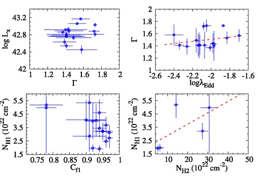
Correlation between different spectral parameters.
On examining the ambient medium surrounding the X-ray emitting region and the column densities along the line of sight, it is generally observed that the X-ray luminosity decreases with an increase in the hydrogen column density (NH i) along the line of sight. As the luminosity is an intrinsic source property and does not depend on absorption due to matter along the line of sight, we do not find any strong correlation or anticorrelation between Lx and NH i. The correlation coefficient is found to be PCC = −0.32 with a (p-value = 0.21). This suggests that the nature of the source remained unchanged, whereas there was a change in the density of the hydrogen cloud. As the column density increases, the amount of hydrogen gas in the ambient medium around the X-ray emitting region is expected to increase. Consequently, we find a correlation between NH i and NH2, with a PCC of +0.64 (p-value = 0.24). This indicates that as the gas density rises in the ambient medium around the central engine, it covers a larger area. This behaviour is reflected in Mrk 6, where we find a strong correlation between NH2 and the ionized gas covering factor |$C^{\xi }_{\rm f}$|, with a PCC of +0.87 (p-value = 0.05). The results of our correlation study are tabulated in Table 9.
Correlation between parameters obtained from the spectral fitting of data from observations with various X-ray observatories over a period of 22 years. Parameter-1 and Parameter-2, shown in the first and second columns, respectively, are involved in the correlation study. The Pearson Correlation Coefficient (PCC) is shown in the third column, and the corresponding p-values are shown in the fourth column. A negative PCC value shows an anticorrelation between the two parameters, whereas the opposite is valid for a positive PCC value.
| Parameter-1 | Parameter-2 | PCC | p-value |
|---|---|---|---|
| Γ | |$\log\lambda_{\rm Edd}$| | +0.42 | 0.09 |
| Γ | |$\log L_{x}$| | +0.41 | 0.10 |
| |$\log L_{x}$| | NH i | −0.32 | 0.21 |
| NH i | NH2 | +0.64 | 0.24 |
| NH2 | |$C^{\xi }_{\rm f}$| | +0.87 | 0.05 |
| Parameter-1 | Parameter-2 | PCC | p-value |
|---|---|---|---|
| Γ | |$\log\lambda_{\rm Edd}$| | +0.42 | 0.09 |
| Γ | |$\log L_{x}$| | +0.41 | 0.10 |
| |$\log L_{x}$| | NH i | −0.32 | 0.21 |
| NH i | NH2 | +0.64 | 0.24 |
| NH2 | |$C^{\xi }_{\rm f}$| | +0.87 | 0.05 |
In this study, we explore the correlation between different parameters and find that the variation of these parameters can be explained from the physical point of view. However, it is important to note that the p-value associated with some correlation is greater than 0.05, indicating that the correlation may not be statistically significant at the 5 per cent level. This suggests that the observed relationship could potentially be due to random variability. Further investigation or a larger sample size may be needed to draw more accurate conclusions. Photon index (Γ), which is directly measured from a simple power-law fitting to the X-ray spectrum, is related to other physical quantities such as X-ray continuum luminosity (Lx) and/or Eddington ratio (λEdd) of the source. The neutral hydrogen column density along the line of sight (NH i) is also found to be non-variable and correlated with the ionized hydrogen column density (NH2) of this source. These correlations and anticorrelations between different parameters provide valuable insights into the behaviour of the X-ray emitting region in Mrk 6 and are consistent with known trends observed in other AGNs. We successfully explain their behaviour using the correlations and anticorrelations between them. This result provides a better understanding of the complex behaviour of Mrk 6.
5 CONCLUSIONS
We conducted a detailed temporal and spectral analysis of the X-ray observations of Mrk 6 over a time period of ∼22 years (2001–2022). During this observation period, we observe a minor variation in the various spectral parameters of this source, such as photon index, X-ray luminosity, and Eddington ratio. We explored the nature of obscuring materials of this source and tried to understand its complex nature. Furthermore, our analysis of the broad-band spectrum unveiled insights into the properties of the reflecting medium, allowing us to estimate the intrinsic parameters like the inclination angle and torus opening angle. In this summary, we present an outline of our key findings.
Although Mrk 6 displays characteristics of a changing-look AGN (CLAGN) from optical observation in the past, our X-ray spectral analysis shows a marginal variation in the X-ray luminosity and Eddington ratio over a period of 22 years. This indicates that in the X-ray regime, the source did not show any significant change in its behaviour during the observational period. It is noted that the X-ray continuum luminosity varies between 3 × 1042 to 15 × 1042 erg s−1, and the corresponding Eddington ratio changes from 0.004 to 0.020 in the 22 years of the observational period. Based on the calculated Eddington ratio, it is evident that the source remains in a sub-Eddington regime during these observations.
We observed a complex variable structure of the obscuring absorber of Mrk 6. The hydrogen cloud, relatively closer to the central engine, appears partially ionized and extends up to NLR or the Torus region. This section of the cloud displays complex variability and undergoes rapid temporal changes. We observed this component of the hydrogen cloud up to the 2015 observations and predicted that it would have disappeared between 2015 and 2019. In contrast, another portion, situated far from the central engine, remained relatively stable over time. It is important to note that the torus did not have a direct impact on the X-ray observations, as the torus opening angle is significantly larger than the inclination angle.
Correlation study of light curves in soft (0.5–3.0 keV range) and hard (3.0–10.0 keV range) bands yielded a fairly strong correlation with approximately zero delay for long-term observations. The detection of this correlation suggests that the photons in both energy bands originate from the same physical mechanism. However, in the shorter time-scale (a few ks), we observed only a weak correlation or no correlation between these two energy bands. On the other hand, in the high energy band (above 10 keV), we did not notice any significant correlations with different energy bands. It is important to note that a strong correlation between the soft and hard bands exists when the structure of column density is relatively simpler.
From the temporal study, we report that the fractional rms amplitude (Fvar) of the source is below 10 per cent for the shorter time-scale (∼60 ks) and above 20 per cent for longer time-scale (∼weeks).
ACKNOWLEDGEMENTS
We sincerely thank the anonymous referee for his/her insightful comments and constructive suggestions that helped us to improve the manuscript. The research work at the Physical Research Laboratory, Ahmedabad, is funded by the Department of Space, Government of India. The data and/or software used for this work is taken from the High Energy Astrophysics Science Archive Research Center (HEASARC), which is a service of the Astrophysics Science Division at NASA/GSFC and the High Energy Astrophysics Division of the Smithsonian Astrophysical Observatory. This work has made use of data obtained from the NuSTAR mission, a project led by Caltech, funded by NASA, and managed by NASA/JPL, and has utilized the NuSTARDAS software package, jointly developed by the ASDC, Italy, and Caltech, USA. This work has used data from the Suzaku, a collaborative mission between the space agencies of Japan (JAXA) and the USA (NASA). This work made use of data Swift/XRT supplied by the UK Swift Science Data Centre at the University of Leicester. This research has made use of observations obtained with XMM–Newton, an ESA science mission with instruments and contributions directly funded by ESA Member States and NASA.
DATA AVAILABILITY
We used archival data of Swift/XRT, XMM–Newton, Suzaku, and NuSTAR observatories for this work. These data are publicly available on their corresponding websites. Appropriate links are given in the text.
Footnotes
|${\rm borus02\_v170323c.fits}$|s
