


ABSTRACT
We explore the eccentricity measurement threshold of Laser Interferometer Space Antenna (LISA) for gravitational waves radiated by massive black hole binaries (MBHBs) with redshifted BH masses Mz in the range 104.5–107.5 M⊙ at redshift z = 1. The eccentricity can be an important tracer of the environment where MBHBs evolve to reach the merger phase. To consider LISA’s motion and apply the time delay interferometry, we employ the lisabeta software and produce year-long eccentric waveforms using the inspiral-only post-Newtonian model taylorf2ecc. We study the minimum measurable eccentricity (emin, defined one year before the merger) analytically by computing matches and Fisher matrices, and numerically via Bayesian inference by varying both intrinsic and extrinsic parameters. We find that emin strongly depends on Mz and weakly on mass ratio and extrinsic parameters. Match-based signal-to-noise ratio criterion suggest that LISA will be able to detect emin ∼ 10−2.5 for lighter systems (Mz ≲ 105.5 M⊙) and ∼10−1.5 for heavier MBHBs with a 90 per cent confidence. Bayesian inference with Fisher initialization and a zero noise realization pushes this limit to emin ∼ 10−2.75 for lower-mass binaries, assuming a <50 per cent relative error. Bayesian inference can recover injected eccentricities of 0.1 and 10−2.75 for a 105 M⊙ system with an ∼10−2 per cent and an ∼10 per cent relative errors, respectively. Stringent Bayesian odds criterion (|$\ln {\mathcal {B}}\gt 8$|) provides nearly the same inference. Both analytical and numerical methodologies provide almost consistent results for our systems of interest. LISA will launch in a decade, making this study valuable and timely for unlocking the mysteries of the MBHB evolution.
1 INTRODUCTION
The Laser Interferometer Space Antenna (LISA; Amaro-Seoane et al. 2017; Barack et al. 2019) will be one of the first space-based gravitational wave (GW) observatories that will launch in the 2030s, along with TianQin (Wang et al. 2019) and Taiji (Gong et al. 2021). It will be sensitive to observed frequencies of GWs in the range of ∼10−4–10−1 Hz. The primary extragalactic sources for LISA are mergers of massive black hole binaries (MBHBs) of 104–108 M⊙ and intermediate/extreme mass ratio inspirals (I/EMRIs; Babak et al. 2017; Amaro-Seoane 2018b) with primary-to-secondary BH mass ratio q greater than 103. LISA will be sensitive enough to detect GWs from coalescing MBHBs with q ≲ 10.0 up to redshift z ∼ 20 (Amaro-Seoane et al. 2017). Most MBHBs will have high signal-to-noise ratios (SNRs; Amaro-Seoane et al. 2017) in the LISA band, which will help to constrain their parameters with high accuracy.
MBHBs mainly form as by-products of galaxy mergers (Begelman, Blandford & Rees 1980). The process involved in shrinking the separation between MBHs from galactic scales to form a binary in the post-merger nucleus takes millions to billions of years, depending on the internal structure of the host galaxies and the relative dominance of various astrophysical processes (see, e.g. Amaro-Seoane et al. 2023). At sub-pc scales, the interaction of the binary with gas and stars in its environment can drive the binary to the coalescence phase in the LISA band within a Hubble time (Milosavljević & Merritt 2003; Haiman, Kocsis & Menou 2009). By the time a tight binary is formed, information on its dynamical history, which reflects the nature of the properties of the host galactic nucleus, is mostly lost. However, GW waveforms from these tight systems can carry signatures of the source environment, either in the form of modifications of the vacuum waveform, from phase shifting (Barausse, Cardoso & Pani 2014; Derdzinski et al. 2019, 2021; Toubiana et al. 2021; Cardoso et al. 2022; Sberna et al. 2022) and amplitude modulation (D’Orazio & Loeb 2020) to the injection of additional harmonics at higher frequency (Zwick et al. 2022), or via a direct relation with the binary parameters that can be extracted from the analysis of the vacuum waveform. In the latter case, the precise astrophysical environment an MBHB evolves within from pc-scales to the near-merger stage may lead to different system variables at the LISA entry for the same starting binary.
One of the most sensitive binary parameters to the surrounding environment is the orbital eccentricity. While most studies in the literature assume that MBHBs will circularize by the time they enter the LISA band (with entry eccentricity eLISA ≲ 10−4) due to emission of GWs (Peters & Mathews 1963; Peters 1964), some may retain non-negligible eccentricity due to evolving in a suitable dynamical environment, e.g. if MBHBs are embedded in gas (Armitage & Natarajan 2005; Sesana et al. 2005; MacFadyen & Milosavljević 2008; Cuadra et al. 2009; Roedig et al. 2011; Roedig & Sesana 2012; Siwek, Weinberger & Hernquist 2023; Tiede & D’Orazio 2023), in a star cluster (Matsubayashi, Makino & Ebisuzaki 2007; Löckmann & Baumgardt 2008; Preto et al. 2009; Sesana 2010; Gualandris et al. 2022), in a tri-axial potential (Merritt & Vasiliev 2011; Khan et al. 2013), or if they interact with a third BH (Bonetti et al. 2016, 2018a, b, 2019). Hence, eccentricity can be an important tracer to probe these effects.
The eccentricity is a unique intrinsic binary parameter because it decreases rapidly as the system approaches the merger. As a result, in order to infer it from a waveform, we need to detect the GW signal many cycles before the merger. Therefore, for now, the ground-based LIGO-Virgo-KAGRA (LVK) collaboration does not include eccentricity in their analysis of the stellar-mass (≲100 M⊙) BH binaries (SmBHBs) due to the challenges in modelling late-inspiral-merger with the presence of eccentricity and spins (see, e.g. Ramos-Buades et al. 2022). However, LVK indeed does searches for eccentric SmBHBs using un-modelled methods (Abbott et al. 2019; Ramos-Buades et al. 2020). Given that we will observe GWs in the early inspiral phase in the LISA band for most MBHBs, ignoring eccentricity could lead to mismodelling of the GW waveform. Most of the focus on eccentricity detection in the LISA frequency band has been in the context of multi-band SmBHBs sources (Nishizawa et al. 2016, 2017; Klein et al. 2022), with some attention on EMRIs. Multi-band sources are seen in the LISA band a few years before they merge in the LVK frequency band of ∼10–104 Hz (Sesana 2016; Vitale 2016). The detection of eccentricity is proposed as a way to distinguish whether SmBHBs are formed in the field or via dynamical interaction such as in globular clusters, nuclear clusters, or galactic nuclei (Breivik et al. 2016; Nishizawa et al. 2016; D’Orazio & Samsing 2018; Gondán et al. 2018; Samsing & D’Orazio 2018; Romero-Shaw, Lasky & Thrane 2019, 2022; Romero-Shaw et al. 2020; Zevin et al. 2021). Also, eccentricity can help in breaking parameter degeneracies by inducing higher harmonics (Mikóczi et al. 2012; Yang et al. 2022; Xuan; Naoz & Chen 2023) and it can improve parameter estimation accuracy (Sun et al. 2015; Vitale 2016; Gondán et al. 2018; Gondán & Kocsis 2019; Gupta et al. 2020). EMRIs are mostly expected to have a significant entry eccentricity in the LISA band, ranging from eLISA ≳ 0.1–0.8 (Hopman & Alexander 2005; Amaro-Seoane 2018a), which can be measured to high accuracy, barring data analysis challenges (Babak et al. 2017; Berry et al. 2019; Chua & Cutler 2022).
This work considers eccentric binaries in vacuum of two near-coalescence non-spinning MBHs. We are interested in determining the minimum eccentricity that can be confidently measured by LISA one year before the merger for a given MBHB source at z = 1. Our analysis attempts to be as realistic as possible in the data analysis which will be employed for LISA once the mission is operational, i.e. we take into account the full LISA motion in its orbit around the Sun, generate high-order post-Newtonian (PN) waveforms, employ the time delay interferometry (TDI) technique to cancel the detector’s laser noise, and finally perform Bayesian inference to recover injected parameters.
The measurability of eccentricity in the MBHB’s GW waveform is a novel investigation. It is an important study because, similar to multi-band sources, residual eccentricities can be a signature of the environment in which MBHBs have evolved. For instance, recent high-resolution hydrodynamical simulations by Zrake et al. (2021) show that for equal-mass binaries hardening in prograde circumbinary gas discs, we expect an eccentricity of ∼10−3 one year before coalescence. The eccentricity evolution in the late stages of hardening by a prograde accretion disc is further supported by D’Orazio & Duffell (2021) and Siwek, Weinberger & Hernquist (2023). Moreover, Tiede & D’Orazio (2023) show that we should expect even higher eccentricity in the LISA band if the circumbinary disc is retrograde instead of prograde. Therefore, eccentricity detection by LISA could be a tracer of gas interaction. Simulations of MBH binary evolution starting from realistic galaxy mergers (Capelo et al. 2015), in which three-body encounters with stars dominate the orbital decay at sub-pc separations, show that the eccentricity always increases above the value that it has when the hardening phase begins, reaching values as large as 0.9 (Khan et al. 2018). The residual value of eccentricity around 50–100 Schwarzschild radii (about one year before merger), when circularization via GW emission has already started to act, is yet to be determined. However, recently Gualandris et al. (2022) studied the evolution of eccentricity through the stellar hardening phase and into the GW radiation regime, finding that the residual value of the eccentricity at about 50 Schwarzschild radii for a 4 × 10⁶ M⊙ MBHB ranges from below 10−4 to nearly 10−3 (as suggested by Elisa Bortolas in further communication). Interestingly, the specific eccentricity here mainly depends upon the parameters at large scale and positively correlates with the initial eccentricity of the merging galaxies. Also, the lowest possible eccentricity detectable by LISA for a given MBHB will tell us whether its neglect during parameter estimation will lead to biases and degeneracies. The consensus for entry eccentricity in the LISA band for MBHBs is ≲10−4, which justifies the circular assumption, but for eLISA > 10−4, it would be crucial to consider eccentricity during match filtering and when constraining binary variables (Porter & Sesana 2010).
The paper is structured as follows: In Section 2, we describe our waveform model and systems of interest. Section 3 studies analytical constraints on eccentricity measurement using matches and Fisher formalism. In Section 4, we detail our Bayesian setup to find the minimum measurable eccentricity. We discuss the findings in Section 5 and summarize the key takeaways of this work in Section 6.
2 WAVEFORM GENERATION, SYSTEM PARAMETERS, LISA RESPONSE, AND TIME DELAY INTERFEROMETRY
MBHBs are one of the most promising sources for LISA as they are expected to be the loudest events and will spend a significant amount of time (up to a few years) in LISA’s frequency band before merging. Most of the time MBHBs spend in the LISA band is in the long-inspiral phase where eccentricity (e) can still be non-negligible. The inspiral part of the GW waveforms from eccentric BHB mergers has been developed within the PN formalism both in time and frequency domains (Damour, Gopakumar & Iyer 2004; Mishra et al. 2016). The time-domain PN waveforms have the advantage of having a larger region of validity in eccentricity, and they can probe eccentricities up to ≈0.8, but they are slow to generate (Tanay, Haney & Gopakumar 2016; Tanay et al. 2019). The frequency-domain waveforms are much faster to compute but are limited to the low-eccentricity approximation. For LISA data analysis, it is imperative to have fast waveform computation as the evolution of the BHB occurs over a large time-frequency volume. There exist a wide range of frequency-domain eccentric BHB waveforms, namely taylorf2ecc (Moore et al. 2016), EccentricFD (Huerta et al. 2014), and EFPE (Klein 2021), among others. For this study, we have employed the taylorf2ecc inspiral-only waveform model with circular phasing accurate up to 3.5PN order taken from another inspiral-only model taylorf2 (Buonanno et al. 2009) and eccentricity corrections to phasing up to 3PN and |$\mathcal {O}(e^2)$|, making it valid for e ≲ 0.1. However, this model does not give a prescription for spinning BHs. We choose TaylorF2Ecc as our fiducial model as astrophysically we mostly do not expect higher eccentricities, as mentioned in the introduction.
The parameter space we consider for MBHBs spans the range of total redshifted masses Mz between 104.5 and 107.5 M⊙, mass ratios.1q ∈ [1.2, 8], and the initial eccentricity one year before the merger (e1yr) between 10−3.5 and 0.1. We have not considered the individual spins of the component BHs for this work. Unless otherwise stated, we always quote the values at the detector frame (L-frame). This leaves us with three intrinsic parameters2 (first three rows of Table 1) and six extrinsic parameters (last six rows of Table 1). We employ the cosmological parameters from the Planck Collaboration VI (2020) survey to compute the luminosity distance from redshift: Hubble constant H0 = 67.77 km s−1 Mpc−1, matter density parameter Ωm = 0.30966, and dark-energy density parameter ΩΛ = 0.69034.
Source parameters in the L-frame.
| Parameter | Units |
|---|---|
| Total redshifted mass Mz | M⊙ |
| Mass ratio q | Dimensionless |
| Eccentricity one year before coalescence e1yr | Dimensionless |
| Luminosity distance DL | Mpc |
| Phase at coalescence ϕ | Radian |
| Inclination ı | Radian |
| Ecliptic latitude λ | Radian |
| Ecliptic longitude β | Radian |
| Initial polarization angle ψ | Radian |
We generate eccentric waveforms |$\tilde{h}_{\rm ecc}(f)$| for our systems of interest using the taylorf2ecc template over these parameter grids to optimally cover the intrinsic parameter space:
Additionally, we also generate quasicircular (e1yr = 0) waveforms (|$\tilde{h}_{\rm cir}$|). For extrinsic parameters, our fiducial values are z = 1 which corresponds to DL = 6791.3 Mpc, and the angles are all set to 0.5 radians. We choose these parameters such that MBHBs spend at least one year in the LISA band before coalescing.
In this work, we only work with Newtonian amplitudes and study binaries until they reach their innermost stable circular orbit (ISCO), i.e. at binary separation rISCO ≡ 3rs, where rs ≡ 2GMz/c2 is the Schwarzschild radius of the total mass BH,3 at which point binaries are expected to circularize.4 We find the starting frequency (f1yr) such that the system reaches the ISCO at frequency fISCO in exactly one year by using the Peters’ time-scale (Peters 1964). The reason why we have chosen f1yr as our reference frequency to initiate the signal and not some fixed frequency as usually employed by the LVK collaboration is that MBHB masses can vary by up to three orders of magnitude, making any fixed frequency sufficient for some systems and too short or long for others.
In Fig. 1, we show the characteristic strain |$h_{\rm c}(f)\equiv 2f\tilde{h}(f)$|, a visual aid to represent how signal adds up in the detector, the LISA noise curve Sn(f) including a confusion noise due to galactic binaries taken from Marsat, Baker & Canton (2021), and the accumulated phase for an Mz = 105 M⊙, q = 8.0, and e1yr = 0.1 system at z = 1 for taylorf2ecc and the quasicircular inspiral-merger-ringdown waveform model IMRPhenomD (Husa et al. 2016; Khan et al. 2016). Since the inspiral part of the IMRPhenomD comes from the taylorf2 template, phasings are almost identical until the system is close to the ISCO. The initial phase difference is due to non-zero eccentricity in taylorf2ecc, and later deviations come from the merger part of the IMRPhenomD, which are beyond the scope of the inspiral-only model taylorf2ecc.
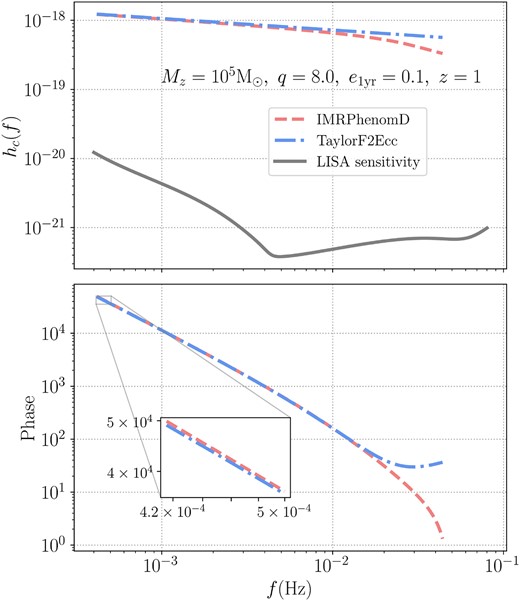
Characteristic strain hc compared to the LISA noise (solid grey; in the top panel) and accumulated phase (in the bottom panel) for an Mz = 105 M⊙, q = 8.0, and e1yr = 0.1 binary at z = 1 for waveform templates IMRPhenomD (dashed red) and taylorf2ecc (dot–dashed blue) between f1yr and fISCO. In the bottom panel, we also enlarge the initial phase to show the difference between quasicircular and eccentric phasings.
To account for LISA motion and to project the waveform into TDI channels, namely A, E, and T, we modify the lisabeta software (see Marsat, Baker & Canton 2021 for details and subsequent notations) by including support for taylorf2ecc. Therefore, a waveform |$\tilde{h}(f)$| will have strain projections |$\tilde{h}_{\rm A,E,T}(f)$| and noise power spectral densities |$S_\mathrm{ n}^{\rm A,E,T}$| corresponding to A, E, and T channels, respectively.
Now, we can write down the standard inner-product between two waveforms as
where the pre-factor 4 comes from the one-sided spectral noise density normalization. Hence, the SNR of the signal is |$\sqrt{(h|h)}$|. In Fig. 2, we show the dependence of the SNR at z = 1 as a function of total mass and mass ratio for our parameter space in equation (1). As expected, the SNR is higher for near-equal mass ratios than the unequal ones and decreases as the redshift increases. Furthermore, the SNR peaks at middle-range masses of ∼106 M⊙, known as golden LISA sources.
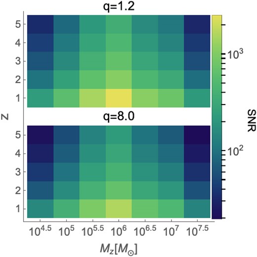
SNR for our systems of interest for two limiting mass ratios of q = 1.2 (top panel) and q = 8.0 (bottom panel). In both panels, we vary Mz from 104.5 to 107.5 M⊙ and z from 1 to 5, and set rest of the parameters to our fiducial values. These SNRs take into account LISA motion and are calculated by summing over three TDI channels A, E, and T. The low eccentricities we consider here do not affect the SNR significantly.
In the following two sections, we find the minimum eccentricity and errors on its recovery in the LISA data stream for a given source. First, we approach this task analytically by using a match between waveforms and computing Fisher information matrices. We then perform Bayesian inference to numerically determine the posteriors.
3 ANALYTICAL MEASURABILITY OF ECCENTRICITY
We first present a simple and commonly used estimate for the distinguishability of eccentric from quasicircular binaries in LISA using a match-based SNR criterion defined in equation (5). Furthermore, we employ the Fisher formalism to estimate how well-constrained eccentricity will be for these sources. These computations provide a theoretical benchmark that can be compared with Bayesian inference presented later.
3.1 Optimal match
We compute matches between hecc and hcir waveforms with the same Mz and q, and find the minimum SNR (SNRmin) for which LISA can distinguish between these waveforms with more than 90 per cent confidence. To compute SNRmin, we use the criterion from Baird et al. (2013):
where |$\chi _k^2(1-p)$| is the χ2 probability distribution function, 1 − p is the significance level, k is the number of free binary parameters, and |$\mathscr {M}(h_{\rm ecc},h_{\rm cir})$| is a match between hcir and hecc:
which is maximized over phase shifts Δϕ. In our case, we have p = 0.9 and k = 3 as we vary only three binary parameters – Mz, q, and e1yr. This transforms equation (3) into
If the event’s SNR is less than SNRmin then one cannot differentiate between quasicircular and eccentric binaries, which in turn provides a constraint on the minimum detectable eccentricity (emin) assuming the rest of the binary parameters are known. In Fig. 3, we show SNRmin for our systems of interest and compare it with the event’s SNR at our fiducial z = 1 (SNRz = 1). It illustrates that emin ∼ 10−2.5 for lower-mass MBHBs (Mz ≲ 105.5 M⊙) and ∼10−1.5 for higher-mass systems. The strong dependence on the total mass can be attributed to the fact that even though our considered binaries spend one year in the LISA band, f1yr for heavier systems is much lower than for the lighter binaries. This implies that the inspiral part of the signal, where eccentricity is dominant, will fall within the low sensitivity region of LISA, leading to systematically worse constraints for heavier systems. Moreover, the weak dependence on the mass ratio can be explained from our definition of e1yr. Unsurprisingly, higher eccentricities are easily distinguishable from lower ones.
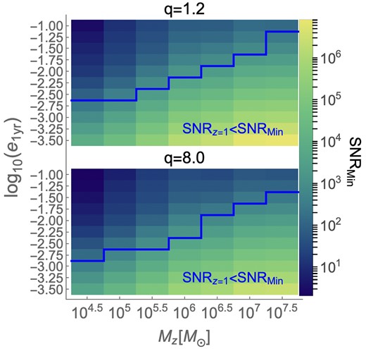
SNRmin required to distinguish between quasicircular and eccentric waveforms for our parameter space. In the top panel, we fix q = 1.2, and vary Mz from 104.5 to 107.5 M⊙ and e1yr from 10−3.5 to 10−1. In the bottom panel, we keep the mass ratio q = 8.0 constant, and vary Mz and e1yr as in the top panel. Both panels have a blue line showing the boundary of the LISA non-detectability region at z = 1 (SNRz = 1 < SNRmin).
One can use the SNR estimates in Fig. 2 for any MBHBs at higher redshift in the LISA band and use Fig. 3 to assess whether eccentricity will be detectable for the given system since SNRmin is computed in the L-frame. In the next section, we find the expected error bars on the recovery of injected eccentricity using the Fisher formalism.
3.2 Fisher matrix
A standard parameter estimation technique in the LISA community is to compute a Fisher matrix (Vallisneri 2008), which tells us how well we can constrain a certain parameter assuming a Gaussian noise and high SNR. We can define the Fisher matrix as
where |$\partial _{\rm a} h\equiv \partial h/\partial \theta _{\rm a}$| is the partial derivative of a waveform h with respect to a parameter θa.
The inverse of the Fisher matrix is the variance–covariance matrix, whose diagonal elements are variances (σ2) for each of the injected parameters. The square-root of a variance provides the standard deviation (σ), which tell us the error estimate on a given parameter.
We again only vary intrinsic parameters: Mz, q, and e1yr, and show in Fig. 4 the Fisher-based error estimate on eccentricity (|$\sigma ^{\rm Fisher}_{\rm e}$|) for our parameters of interest in equation (1). Errors mainly vary with total mass and less significantly with mass ratio, due to the same reasons as explained for the match results in Section 3.1. Fig. 4 suggests that for lighter systems, higher eccentricities are constrained to error (relative error |$\equiv 100\times \sigma ^{\rm Fisher}_{\rm e}/e$|) ∼10−4 (∼0.1 per cent) whereas for lower e1yr we find |$\sigma ^{\rm Fisher}_{\rm e}\sim 10^{-3}$| (∼1000 per cent). For heavier binaries, errors are ∼10−3 (∼1 per cent) for higher eccentricities and ∼10−1 (105 per cent) for lower e1yr. This suggests that lower eccentricities are completely unconstrained.
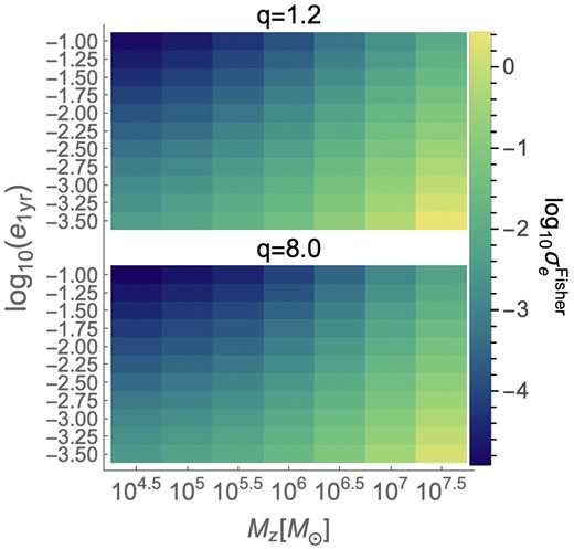
For the same binary parameters as in Fig. 3, error estimates by Fisher formalism (|$\sigma ^{\rm Fisher}_e$|) on eccentricities of our considered binaries.
One can always scale these errors (∼1/SNR) at a further luminosity distance by using SNR values in Fig. 2 to get rough estimates. In the next section, we perform Bayesian inference to find error estimates on eccentricity recovery and the minimum measurable eccentricity.
4 MEASURABILITY OF ECCENTRICITY USING BAYESIAN INFERENCE
The main goal of Bayesian inference is to construct posterior distributions p(θ|d) for the parameter space θ to fit the observed data d (see e.g. Thrane & Talbot 2019). p(θ|d) represents the probability distribution function of θ given the data d and it is normalized such that ∫dθ p(θ|d) = 1. To compute the posterior, we use Bayes theorem,
where |$\mathcal {L}(d|\theta)$| is the likelihood function of the data d given the parameters θ, π(θ) is the prior on θ, and |$\mathit{ Z}\equiv \int {\rm d}\theta \mathcal {L}(d|\theta)\pi (\theta)$| is the evidence. Since we are not selecting between different models, we can treat Z as a normalization constant. Also, we only consider uniform (flat) priors for all parameters.
For our stationary Gaussian noise |$S_\mathrm{ n}^{\mathrm{ A},\mathrm{ E},\mathrm{ T}}$|, we can write down the log-likelihood with a zero-noise realization summed over A, E, and T channels as (Marsat, Baker & Canton 2021):
where |$\tilde{h}$| is the template signal, and |$\tilde{h}_{\rm inj}$| is the simulated injected signal. The zero-noise realization accelerates the likelihood computation, improves upon the Fisher results by providing the shape of posteriors, and helps understand parameter degeneracies and detectability of certain effects (here eccentricity).
For sampling, we use the parallel tempering Markov chain Monte Carlo (MCMC) code ptmcmc.5 To further speed up the likelihood computation, we draw random samples from a multivariate Gaussian with the mean given by the injected parameters and standard deviations provided by the Fisher formalism6 in Section 3.2.
We primarily sample only the intrinsic parameters and set a high-frequency cutoff for the data at fISCO of the injected binary.7 We show the posteriors for Mz, q, and e1yr in Fig. 5 for injected binary parameters 105 M⊙, 8.0, and 0.01. All parameters are well recovered, with the injected values being extremely close to the median of their respective posterior. The chirp mass parameter |$\mathcal {M}\equiv M(q/(1+q)^2)^{3/5}$| is even better constrained to |$24932.3377^{+0.0808}_{-0.0815}~{\rm M}_{\odot }$| as expected (see e.g. Cutler & Flanagan 1994) with the injected value being 24 932.3365 M⊙. Moreover, Bayesian errors are similar to the errors provided by the Fisher formalism, as expected due to the high SNR and a zero-noise realization.
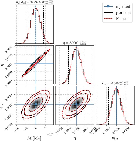
Posterior distributions (solid black) for an injected binary with Mz = 105 M⊙, q = 8.0, and e1yr = 0.01. The extrinsic parameters are fixed to our fiducial values. The two extreme vertical dashed lines constrain the 90 per cent credible interval, whereas the middle dash line represents the median of the distribution. The blue lines mark the injected values, whereas the contours in two-dimensional posteriors indicate 68, 95, and 99 per cent credible intervals. We also indicate the Fisher results (dashed red) for comparison.
We also study the effect of including extrinsic parameters8 (also given in Table 1) on the measurability of the eccentricity in Fig. 6. Here, we show the comparison of the posteriors of e1yr in equation (1) for fixed Mz = 105 M⊙ and q = 8.0 between the cases when sampling only intrinsic parameters and when sampling over all parameters in Table 1. Adding extrinsic parameters results in a slight broadening of eccentricity posteriors and a narrow shift in the peak. This is anticipated due to the increase in degrees of freedom, which do not contribute to the measurement of eccentricity.9 Unsurprisingly, the higher the eccentricity, the better the recovery of the injected value, i.e. the injected value is extremely close to the peak of the posterior.
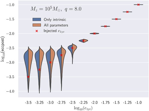
Posterior distributions (eccpost) for the eccentricity corresponding to each injected e1yr for binaries with fixed Mz = 105 M⊙ and q = 8.0. The posteriors are constrained to the 90 per cent credible interval and are shown in blue (left) if we only sample the intrinsic parameters and in orange (right) if we vary all parameters. The injected values are marked with a red cross.
To measure how well injected eccentricities are recovered in our Bayesian inference, we introduce a Bayesian relative error metric in terms of the injected eccentricity einj and the standard deviation of the corresponding eccentricity posterior |$\sigma ^{\rm MCMC}_e$|:
To survey the parameter space widely with Bayesian inference, we have conducted a total of 7 × 4 × 8 runs by sampling over only intrinsic parameters for seven values of the total mass, four values of the mass ratio, and eight values of the eccentricity given in equation (1). We present only the runs for the intrinsic parameters here, as we have shown that including extrinsic parameters does not affect the results significantly.
We present the findings of our Bayesian inference in terms of |$\sigma ^{\rm MCMC}_{e,\rm rel}[\%]$| in Fig. 7. Systems with e1yr ≳ 10−1.5 will mostly lead to the measurement of eccentricity to a relative error of less than 1 per cent for lower-mass MBHBs and ≲10 per cent for higher-mass binaries, independent of q. The lowest value of eccentricity (emin) that LISA can measure with a less than 50 per cent relative error is 10−2.75 for Mz = 104.5 M⊙.
![For the same binary parameters as in Fig. 3, relative error percentage ($\sigma ^{\rm MCMC}_{e,\rm rel}[\%]$) on the recovery of eccentricity in our Bayesian inference. A dashed red line is drawn to separate the region with relative error larger than 10 per cent and a solid blue line is drawn to separate the region with $\sigma ^{\rm MCMC}_{e,\rm rel}[\%]\gt 50$ per cent. We have suppressed relative errors above 100 per cent to enhance the informative results.](https://oup.silverchair-cdn.com/oup/backfile/Content_public/Journal/mnras/528/3/10.1093_mnras_stad3477/1/m_stad3477fig7.jpeg?Expires=1750253248&Signature=Drb28XlUAcQM32I62aBuxw0LzZsb~GpDMkKe65mcA3B9wjcLXSfaJyp0YQOqSqf9VsYAYw8iD8VXyMs6AdmOyhyGrN~AQeukL82tAkZ0utG8nfLVTJPlNShjSnmt8S8NLG1853tSd6jpVR9vnT~vcwDFr7Z6Z425C7BSADFm00NcQC0WiRK20TRJPSGdqe0JPXilwrJ1IDOhCFlXjSpH1D0r5tDgSQ45aaNL3T8PPBzeWvgqJ5ozvfNPwTnwhZKtVDm9L2y15fB0uXMYmxU4z-4XM5NxTy0-YhxB2ugF6aspHxQ82Cc9d-DrkzLecpjcElJ~IkXG1PkA1~rNgIQozQ__&Key-Pair-Id=APKAIE5G5CRDK6RD3PGA)
For the same binary parameters as in Fig. 3, relative error percentage (|$\sigma ^{\rm MCMC}_{e,\rm rel}[\%]$|) on the recovery of eccentricity in our Bayesian inference. A dashed red line is drawn to separate the region with relative error larger than 10 per cent and a solid blue line is drawn to separate the region with |$\sigma ^{\rm MCMC}_{e,\rm rel}[\%]\gt 50$| per cent. We have suppressed relative errors above 100 per cent to enhance the informative results.
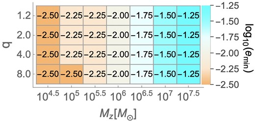
We set 50 per cent Bayesian relative error as a fiducial threshold for the measurement of eccentricity.10 We summarize the results of all our MCMC runs in terms of the minimum measurable eccentricity (emin) by LISA as a function of total mass and mass ratio in Fig. 8. The results are mostly independent of mass ratio, although we witness some slight change for higher-mass ratios (q = 8). emin for heavier systems is around 10−1.5, whereas for lighter MBHBs the eccentricity can be measured down to ∼10−2.75. The measurement of eccentricity in this regime can have far-reaching astrophysical consequences which we present in the discussion.
![Minimum measurable eccentricities as a function of binary mass and mass ratio based on whether $\sigma ^{\rm MCMC}_{e,\rm rel}[\%]\lt 50$ in equation (8).](https://oup.silverchair-cdn.com/oup/backfile/Content_public/Journal/mnras/528/3/10.1093_mnras_stad3477/1/m_stad3477fig8.jpeg?Expires=1750253248&Signature=nkTVUEhtnE~spkfQI1dCZFZ0Q9iIwtPdlN2ciDuQdMQna8j0z2HG1GZJjOcuOf0oCJHFUYYKqXJkLF9nZPqs8R1DdE-Lij2ZSN5YP7VeNJKfYcTxxqvAayBaz7V6siUM8L8yXQwUsmKaEBRPTZ~YJeF~02qbB06mnKNbldzxDzuDuNv9eKSyKvj~LRQMQqN15VmmSXAXzgxOpKvbTddSFBZChiA2Hjz8K0rxxc3AE58KbosFJCBEGvKOaGHh3K9850q~RhSl7gCbGPh9swFl52x86VJF1LzkW0U4MlHUcQvR1J3ZogSDhV2AsBz1UxfWXEUqWIZso1iYjMc979zXUg__&Key-Pair-Id=APKAIE5G5CRDK6RD3PGA)
Minimum measurable eccentricities as a function of binary mass and mass ratio based on whether |$\sigma ^{\rm MCMC}_{e,\rm rel}[\%]\lt 50$| in equation (8).
5 DISCUSSION
The current detectability analysis of GWs from MBHBs mostly assumes negligible eccentricity (≲10−4) once the binaries enter the LISA frequency band. However, we know that environmental interaction is necessary for binaries to reach the near-coalescence phase within a Hubble time. Therefore, it is important to consider if even residual eccentricities are measurable, which can be a tracer of the binary’s environment. In this work, we remain agnostic about the driver of the binary’s eccentricity. Instead, we have determined the minimum measurable eccentricity for a range of binary parameters. These limits can be compared with theoretical models of binary evolution in order to determine which binary formation scenarios lead to measurable eccentric signatures in the GW waveform. For example, we can compare our results with eccentricities predicted by binary evolution in circumbinary discs (D’Orazio & Duffell 2021; Zrake et al. 2021; Siwek, Weinberger & Hernquist 2023), which predict |$e_{1\rm yr}\sim 10^{-3}$| for ∼103–105 M⊙ systems at z = 1. Based on our results in Fig. 8, e ∼ 10−3 will be indeed detectable11 for binaries within the mass range ∼104.5–105.5 M⊙ at z = 1. Considering that the eccentricity evolution will depend on the accretion disc properties (D’Orazio & Duffell 2021), precise detection of eccentricity in GWs can help constrain the source’s environmental properties. The interaction with stars can also excite non-negligible eccentricities in the LISA band. Gualandris et al. (2022) suggest |$e_{1 \rm yr}\sim 10^{-4}$|–10−3 for a 4 × 10⁶ M⊙ MBHB, a range of eccentricities not detectable for such massive system as per Fig. 8. However, lower-mass binaries are not yet explored in these models. It is possible that a better waveform model which includes more physics concerning eccentricity, such as the advance of periastron (Tiwari et al. 2019), could improve eccentricity measurements, but we leave this to future work. Overall, measuring specific eccentricities predicted by various environments may help to distinguish between them. Furthermore, not including eccentricity during parameter estimation could lead to significant biases in the recovery of other binary parameters (see Appendix B).
In addition to measuring orbital properties of binaries in GWs, informative measurements of environmental deviations in GW waveforms are also possible for certain systems. Suppose the influence of scattered stars, surrounding gas, or a nearby third body causes alterations in the orbital evolution (compared to the same binary in vacuum). In that case, this interaction leads to a dephasing of the detected GW signal (e.g. Garg et al. 2022; Zwick, Capelo & Mayer 2023), amplitude modulation due to Doppler boosting and lensing (D’Orazio & Loeb 2020), and can excite harmonics at higher frequencies (Zwick et al. 2022). For a complete characterization of the binary properties in astrophysical environments, it will be necessary to consider how these deviations correlate with binary parameters. Assuming one has a robust knowledge of the range of predicted residual eccentricities in different scenarios for the background (e.g. a gaseous environment versus stellar encounters) and, simultaneously, of the expected waveform modulation due to various interactions, it becomes possible to cross-correlate these parameters to enhance the determination of environmental effects. We plan to quantify the feasibility of these measurements in future work.
LISA and other space-based mHz GW detectors will be able to observe the coalescence of MBHBs in the mass range 104–108 M⊙ across the whole sky. We expect to detect at least a few events per year, with the event rate dominated by lower-mass MBH mergers at z ≲ 2 (Amaro-Seoane et al. 2023). However, current predictions by both post-processing of cosmological simulations and semi-analytical models vary by orders of magnitude, as they depend on intricate details of MBH seeding mechanisms and evolution in their host galaxies (e.g. Ricarte & Natarajan 2018; Tremmel et al. 2018; Barausse et al. 2020; Volonteri et al. 2020; Valiante et al. 2021). While the literature is still evolving on the expected residual eccentricity at LISA entry from different environments, being able to measure the eccentricity might add important information to place further constraints on astrophysical scenarios for binary evolution. Furthermore, irrespective of that, we need to be able to extract all the potential information from the waveform if we are going to use them for fundamental physics tests, such as excluding alternative general relativistic theories (there can be various hidden degeneracies we do not know of at the moment).
The work presented here is not devoid of certain systematics that are present in the GW waveform model that is employed. As mentioned in Section 2, the GW model taylorf2ecc we use only provides eccentric phase corrections up to 3PN and at |$\mathcal {O}(e^2)$|, which makes it reasonable to use in the low-eccentricity regime but can still induce some inaccuracies. The higher-order eccentric corrections – up to |$\mathcal {O}(e^6)$| – are known (Tiwari et al. 2019) but are cumbersome to implement within the full Bayesian inference infrastructure, and the comparison of result for the leading order in eccentricity with respect to higher-order eccentric corrections are left for future work. Additionally, TaylorF2Ecc does not include the component spin effects, which can have positive and negative consequences for the measurability of eccentricity. The spin–orbit and spin–spin couplings, which enter at high PN orders in the phasing, can affect the inspiral significantly (Kupi, Amaro-Seoane & Spurzem 2006; Brem, Amaro-Seoane & Spurzem 2013; Sobolenko et al. 2017). However, we would like to point out that LISA will very well measure spin effects near the late inspiral-merger phase of the MBH binary’s evolution, where the system will be quasicircular for the eccentricities considered here, so any possible degeneracies between spins and eccentricity will be broken. To summarize, for low values of eccentricities, one can ignore the above-mentioned GW modelling issues without drastically changing the final results.
In this work, we only consider eccentricity corrections to phase and not to the amplitude. The eccentricity enters at |$\mathcal {O}(e^2)$| in phase without having a |$\mathcal {O}(e)$| term which could be more important for low eccentricities. Amplitude corrections from higher harmonics induced by eccentricity can include |$\mathcal {O}(e)$| terms. Therefore, it needs to be explored how much the inclusion of amplitude corrections due to eccentricity would improve the eccentricity measurement. Lower-mass MBHBs have a large number of GW cycles in the LISA band, which magnifies the |$\mathcal {O}(e^2)$| terms in the cumulative phase, thereby leading to possibly better measurement of eccentricity from phase than from the amplitude for lighter binaries. Furthermore, Moore et al. (2016) states that for the small eccentricities we consider here, eccentricity corrections to phase are more important than to the amplitude.
6 CONCLUSION
In this work, we study LISA-detectable GWs from eccentric MBHBs in vacuum to find the minimum measurable eccentricity (emin) that can be inferred from the GW waveform. We consider systems that spend at least a year before merging in the LISA frequency band at z = 1 with total redshifted mass Mz in the range 104.5–107.5 M⊙, primary-to-secondary mass ratio q between 1.2 and 8, and initial eccentricity e1yr from 10−3.5 to 10−1. These MBHBs have SNR ∼ 100–2500 (see Fig. 2), allowing us to infer their binary parameters with high accuracy. To robustly estimate emin, we use the inspiral-only post-Newtonian eccentric waveform template taylorf2ecc, and consider LISA’s motion in its orbit around the Sun as well as time delay interferometry to suppress the laser noise by employing the lisabeta software. We approach this analytically via computing matches and Fisher matrices, and numerically via Bayesian inference to find emin for optimally chosen parameter grids in equation (1) to cover our systems of interest. We itemize our findings below.
Considering only three free binary parameters – Mz, q, and e1yr – we find that all approaches suggest that emin mainly depends upon Mz and weakly upon q (see Figs 3, 4, and 7).
The optimal match-based SNR criterion, that distinguishes eccentric and quasicircular waveforms with more than 90 per cent confidence, suggests that emin is ∼10−2.5 for lower-mass MBHBs (Mz ≲ 105.5 M⊙ and ∼10−1.5 for higher-mass systems (see Section 3.1 and Fig. 3).
Relative errors on the recovery of eccentricity provided by the Fisher formalism for lighter systems are ∼0.1 per cent for high eccentricities and ∼1000 per cent for low e1yr. For heavier MBHBs, relative errors are ∼1 per cent for higher eccentricities and 105 per cent for lower e1yr (see Section 3.2 and Fig. 4).
Bayesian inference can constrain e1yr ∼ 10−1.5 to less than 10 per cent relative error for most MBHBs.
Sampling also extrinsic parameters in Table 1 does not affect the eccentricity posterior significantly (see Figs 6 and E2).
Assuming a Bayesian relative error of less than 50 per cent as a threshold for emin, we find that the minimum measurable eccentricity is emin = 10−2.75 for 104.5 M⊙ MBHBs, independent of the mass ratio (Fig. 8).
ACKNOWLEDGEMENTS
AD, MG, and LM acknowledge support from the Swiss National Science Foundation (SNSF) under the grant 200020_192092. ST was supported by the SNSF Ambizione Grant Number: PZ00P2-202204. We acknowledge Stanislav Babak, Pedro R. Capelo, and Jonathan Gair for insightful discussions. We also thank Riccardo Buscicchio, Daniel D’Orazio, Lorenzo Speri, and Jakob Stegmann for useful comments on the manuscript. The authors also acknowledge use of the mathematica software (Wolfram Research Inc. 2021), numpy (Harris et al. 2020), and inspiration drawn from the gwfast package (Iacovelli et al. 2022) regarding the python implementation of TaylorF2Ecc.
DATA AVAILABILITY
The data underlying this article will be shared on reasonable request to the authors.
Footnotes
q = 1 system gives leads to Fisher initialization problems in Bayesian inference, hence we choose q = 1.2 as a representative value.
While there are other eccentricity-related binary parameters, we only focus on the magnitude of eccentricity.
G is the gravitational constant and c is the speed of light in vacuum.
We perform circularization test of taylorf2ecc in Appendix A.
Using a wider prior does not affect results as shown in Appendix D.
Using an earlier cutoff than the ISCO does not significantly affect the posteriors, as shown in Appendix C.
We show the full posteriors in Fig. E2.
Eccentricity is not expected to be correlated to the extrinsic parameters.
See Appendix B for the minimum eccentricity based upon the Bayes factor.
See Fig. E1 for |$e_{1\rm yr}=10^{-2.75}\approx 2\times 10^{-3}$| posteriors.
References
APPENDIX A: CIRCULARIZATION TEST FOR TAYLORF2ECC
To check that the TaylorF2Ecc template is well-behaved, i.e. |$\tilde{h}_{\rm ecc}$| converges to |$\tilde{h}_{\rm cir}$| as the system approaches the coalescence, we compute tidal matches: we divide a signal into equal frequency bins and compute the mismatch (i.e. |$1-\mathscr {M}(h_{\rm cir},h_{\rm ecc})$|) with respect to the cumulative frequency. In Fig. A1, we show the evolution of the mismatch as a function of cumulative frequency for three total masses – {105, 106, and 107} M⊙ – with fixed q = 8.0 and e1yr = 0.1 over 20 frequency bins between |$f_{1\rm yr}$| and fISCO. The figure indeed shows that the mismatch is decreasing as the MBHB approaches its ISCO, showing that taylorf2ecc is well-behaved.
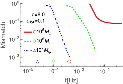
Tidal mismatches for three systems: Mz = 105 M⊙ (solid red), Mz = 106 M⊙ (dashed green), and Mz = 107 M⊙ (dot–dashed blue) for q = 8.0 and |$e_{{1\rm yr}}=0.1$| over 20 frequency bins. We also indicate |$f_{1\rm yr}$| for each respective binary with symbols ○, ⋄, and Δ.
APPENDIX B: BAYES FACTOR AND BIASES
Another way to quantify whether a certain eccentricity is well recovered in our analysis is by computing the Bayes factor. For this purpose, we need to compare two hypotheses which are trying to explain the same eccentric signal. The Null hypothesis is that a circular template (here taylorf2) is enough to accurately describe this signal. The eccentric hypothesis states that you need to have the eccentricity parameter in your template (here taylorf2ecc) to properly explain this signal. We then need to take the ratio of their evidence to compute the Bayes factor
If |$\ln \mathcal {B}\gt 8$| (Lower et al. 2018; Thrane & Talbot 2019), then we have a strong evidence that the given signal comes from an eccentric system rather than a circular one.
To do this we inject eccentric signals using taylorf2ecc and recover them with TaylorF2 to compute Zno ecc and taylorf2ecc to compute Zecc by sampling only intrinsic parameters. Since we are in a zero noise limit and high SNR limit with only eccentricity parameter different between two models, we can compute the Savage-Dickey ratio (Dickey 1971) to approximately get B. We only need to use the Fisher matrix Γij from TaylorF2Ecc for a given injected eccentricity einj :
where Γ ̄ and |${\bar{\Gamma}}$|are determinants of Fisher matrices of all parameters and parameters except eccentricity, respectively, and |$\Gamma^{-1}_{ee}$| is the value of the covariance on eccentricity. Here π(e) = 1/(0.2 − 10−6 ) due to an uniform prior.
In Fig. B1, we show minimum measurable eccentricities if |$\ln \mathcal {B}\gt 8$| for a given Mz and q. These results are almost consistent with Fig. 8, although results slightly worsen due to a stricter criterion.
Same as in Fig. 8, but now based on whether |$\ln \mathcal {B}\gt 8$|.
We can also compute the bias induced in the estimation of Mz and q when fitting circular template to an eccentric signal. For this purpose, we compute the bias for a given parameter θ, normalized by its standard deviation as
where |$\hat{\theta }$| denotes the highest likelihood point in the posterior distribution for the given model, and |$\sigma ^{\theta }_{\rm ecc}$| is the standard deviation of the eccentric model posterior of θ.
In Fig. B2, we show δθ[σ] for Mz and q as a function of varying eccentricity for a fixed Mz = 105 M⊙ and q = 8. Both biases are almost identical and as expected, grow rapidly as |$e_{1\rm yr}$| becomes higher. For |$e_{1\rm yr}=10^{-3.5}$|, the bias in both parameters is ≈0.4 and for |$e_{1\rm yr}=0.1$|, δθ[σ] = 120. These results emphasize the need to included eccentricity during parameter estimation.
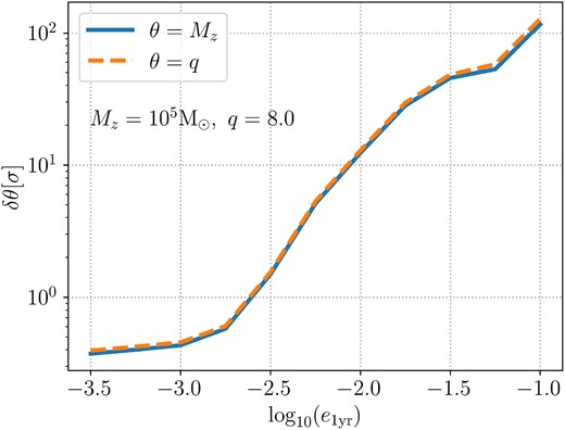
Biases induced in the estimation of Mz and q due to fitting a circular template to an eccentric signal as a function of |$e_{1\rm yr}$| for a system with Mz = 105 M⊙ and q = 8.
APPENDIX C: DEPENDENCE ON HIGH-FREQUENCY CUTOFF
In Fig. C1, we compare posteriors between two signals, where the high-frequency cutoff is at |$10\, r_{\rm s}$| and at our fiducial cutoff |$3\, r_{\rm s}$|. This exercise is performed to ensure that near-merger artefacts, beyond the scope of taylorf2ecc, do not bias our results. Almost overlapping posteriors indeed illustrate that the cutoff near the merger does not affect the recovery of parameters, especially eccentricity, which is an early inspiral effect.
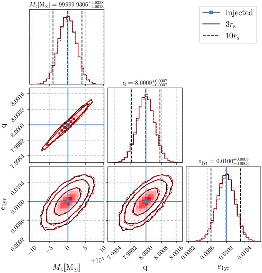
Posterior distributions for the same binary parameters as in Fig. 5 with a high frequency cutoff at |$10\, r_{\rm s}$| (dashed red) binary separation compared to our fiducial cutoff at ISCO or |$3\, r_{\rm s}$| separation (solid black).
APPENDIX D: DEPENDENCE ON FISHER INITIALIZED PRIOR’S COVARIANCE
In Fig. D1, we make a comparison between two posteriors with prior’s covariances either the same as our fiducial Fisher covariances or twice the Fisher covariances. Almost identical posteriors clearly illustrate that our Bayesian runs are giving informative results and not merely giving back the Fisher priors we are using.
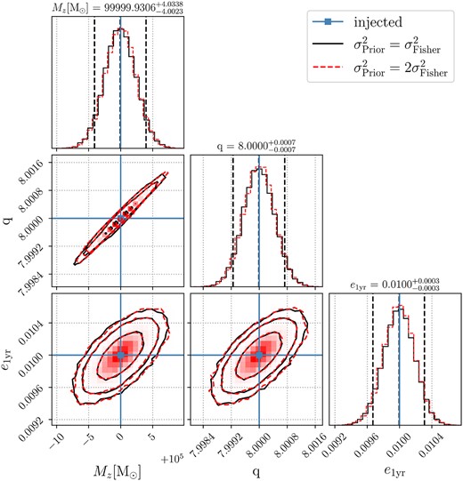
Posterior distributions for the same binary parameters as in Fig. 5 with prior’s covariances (|$\sigma ^2_{\rm Prior}$|) (solid black) being our fiducial covariances (|$\sigma ^2_{\rm Fisher}$|) provided by the Fisher formalism compared to |$\sigma ^2_{\rm Prior}$| set to |$2\sigma ^2_{\rm Fisher}$| (dashed red).
APPENDIX E: SOME INTERESTING POSTERIORS
Fig. E1 shows posteriors for intrinsic parameters for injected MBHB parameters Mz = 105 M⊙, q = 8.0, and e1yr = 10−2.75, a system that is motivated astrophysically by the binary’s interaction with its environment. While the mass and the mass ratio are still well-measured as in Fig. 5 due to similar SNR, eccentricity posterior is broad. Nonetheless, the peak of the eccentricity posterior is very close to the injected value.
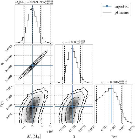
Same as Fig. 5, but for an injected binary with Mz = 105 M⊙, q = 8.0, and e1yr = 10−2.75.
In Fig. E2, we show posteriors for all parameters given in Table 1 for an injected binary with Mz = 105 M⊙, q = 8.0, and e1yr = 0.01 and the extrinsic parameters set to our fiducial values. Comparison with posteriors when only varying intrinsic parameters suggest that while Mz and q are about order-of-magnitude less constrained, eccentricity is almost not affected due to the inclusion of extrinsic parameters, supporting inference from Fig. 6. As expected, there is a degeneracy between the inclination (ı) and the luminosity distance (DL). The phase at coalescence (ϕ) and the polarization angle (ψ) have multi-modality due to periodic functions and hence their injected values are not recovered robustly. The ecliptic latitude (λ) and longitude (β) exhibit slight degeneracies with DL but are well constrained.

Posteriors (solid black) for the same intrinsic binary parameters as in Fig. 5 with sampling included for the extrinsic parameters. We also include posteriors (dashed red) when only sampling intrinsic parameters for comparison.
