The miniJPAS survey. Multiwavelength exploration of detected Extreme Emission Line Galaxies

ABSTRACT

1 INTRODUCTION

Extreme emission line galaxies (EELGs) are a subsample of extra-galactic objects, whose thorough understanding remains elusive. These exceptional astronomical entities, which may seem irrelevant at first sight due to their faint nature and reduced dimensions, might hold the key to our understanding of galaxy formation.

Typically, EELGs are highly compact objects with vivid blue/green colours, being characterized by very high (frequently reaching three orders of magnitude) equivalent widths (EW) of relatively high-excitation emission lines indicative of intense and ongoing star-formation (SF), such as Hα, optical [O iii], and [O ii] or Ly-α when observed at higher redshifts, where they are more frequently detected (e.g. Kunth & Sargent 1986; Erb et al. 2016). By presently harbouring the most violent SF events in the Universe, these galaxies provide a window to the past, resembling epochs where global SF was at its zenith (e.g. Amorín et al. 2015; Pérez-Montero et al. 2021). They produce a substantial amount of photoionizing radiation originated from complexes of young, massive stars, which, although controversial (Loeb & Barkana 2001; Bosch-Ramon 2018), is considered by various authors to significantly contribute to the re-ionization of the Universe (e.g. Salvaterra, Ferrara & Dayal 2011; Dressler et al. 2015; Erb et al. 2016). In addition, this kind of galaxies are acknowledged as likely being the building blocks of local, more massive galaxies (Dressler et al. 2011), and are amidst the most metal-poor objects observed in the Universe (e.g. Kunth & Östlin 2000; Papaderos et al. 2008, for a review). Wolf–Rayet features are often identified in these galaxies (e.g. Schaerer, Contini & Pindao 1999; Amorín et al. 2012). They might be classified as strong He ii emitters (e.g. Kehrig et al 2018; Fernández et al. 2021) and, depending upon the adopted selection criteria and redshift at which they are observed, as blue compact galaxies or blue compact dwarfs (BCGs/BCDs; e.g. Thuan & Martin 1981; Loose & Thuan 1986; Kunth & Sargent 1986; Papaderos et al. 1996; Cairós et al. 2001; Reverte et al. 2007), green pea galaxies (GPGs; Cardamone et al. 2009; Amorín et al. 2015), blueberries (Yang et al. 2016) and/or ELdots (Bekki 2015).

Reviewing the vast complexity of the subject and the broad scientific framework that these exceptional galaxies comprehend, the identification of a statistically meaningful sample across redshift is of uttermost importance. Such will allow to pursue a thorough study of the nature of these objects, and ultimately portray a coherent narrative of their role in the broader context of galaxy formation and evolution. There are several essays attempting for the assembly of a representative sample of EELGs across redshift, such as, e.g. van der Wel et al. 2011 (70 galaxies in the CANDELS fields at z ∼ 1.7), Amorín, Pérez-Montero & Vílchez 2010 (∼180 galaxies from the 20k zCOSMOS bright survey with 0.11 ≤ z ≤ 0.93) or Pérez-Montero et al. 2021 (∼2000 galaxies in the SDSS-DR7 with 0 ≤ z ≤ 0.49) and Lumbreras-Calle et al. 2021 (466 EELGs at z < 0.06) using objective prisms to identify strong emission lines. From these studies, it was disclosed that EELGs display compact morphologies (with R₅₀ ≤ 2 kpc), and a broad range of stellar masses (6.5 ≤ log M_⋆/M_⊙ ≤ 10), with higher masses being mostly found at higher redshifts. Quite importantly, some of these galaxies exhibit pristine environments (e.g. Izotov, Thuan & Guseva 2012; Griffith et al. 2011), with oxygen abundances ranging from 12 + log O/H = ∼7.3 to 8.6, and nitrogen-to-oxygen ratios from ∼0.01 to 0.1. Additional works have provided further insight on this galaxy type. For instance, Maseda et al. (2013, 2014) has analysed two samples of 19 and 22 EELGs detected at 1.3 ≤ z ≤ 2.3, revealing that these have low stellar masses (10⁸–10⁹ M_⊙) and are experiencing intense starbursts. Additional studies have found similar results, such as the works by Tran et al. (2020), Gupta et al. (2021), Gupta et al. (2023), which explores data from the MOSEL survey, covering a sample of strong [O iii] 5007 Å emitting galaxies at 3 ≤ z ≤ 4 extracted from the ZFOURGE survey. Furthermore, by analysing the physical properties of 19 EELGs identified in the ZFOURGE survey, Cohn et al. (2018) revealed that these galaxies show evidence of a starburst in the most recent 50 Myr, assembling 15 per cent of their total stellar mass within this short time period, a highly significant value when contrasted with typical star-forming galaxies, which in the same time period have formed only 4 per cent of their total stellar mass. In addition, Gupta et al. (2021, 2023) have identified signatures of galactic-scale outflows, attributing the pronounced emission lines to interactions and/or mergers. EELGs with even lower stellar masses and higher sSFRs have been identified by Tang et al. (2019) at 1.3 ≤ z ≤ 2.4, ranging from 10⁷ to 10⁸ M_⊙. In addition, these authors have detected O32 values associated with significant Lyman continuum escape.

An excellent opportunity to keep expanding the acquired knowledge on this galaxy genus, and to enlarge the number of these galactic specimens, resides on the exploration of the Javalambre-Physics of the Accelerating Universe Astrophysical Survey (JPAS; Bonoli et al. 2021). Such survey is highly suitable for this purpose, considering that it will observe a vast section of the sky (∼8000 deg²) by means of 54 narrow band filters in the optical regime with an average full width at half maximum (FWHM) of 145 Å (translated into an R of ∼60) and an average spatial resolution with a FWHM < 1.5 arcsec, spanning from 3780 to 9100 Å, and two additional broad filters extending to the ultra-violet (UV) and near infra-red (NIR). It will yield, when complete, one of the largest repositories of photospectra or low (spectral) resolution integral field spectroscopy for all morphological galaxy types from the local Universe up to z ∼ 1. Moreover, past studies have demonstrated that via this photometric survey, one can efficiently identify and characterize emission line galaxies up to z < 0.35 (Martínez-Solaeche et al. 2021, 2022) and the evolution of both red and blue galaxy populations since z = 1 (González Delgado et al. 2021, 2022). Low and intermediate redshift QSOs should be also easily detected (Queiroz et al. 2022) as well as extended Lyman alpha QSOs (Rahna et al. 2022). However, for the correct identification of such elusive objects as EELGs, given their low surface brightness stellar continuum and the similarity with QSOs when observed through the filter scheme of JPAS, our team developed an efficient technique that identifies EELGs candidates by searching for especially strong EW emission lines (EW ≥ 200 Å). This method (Iglesias-Páramo et al. 2022, hereafter IP22) was tested using the data released by the miniJPAS survey (covering 1 deg² of the AEGIS field), having identified 20 EELGs and 11 QSO candidates.

This article describes the characterization of the EELGs & QSOs identified by the aforementioned tool, outlining the development of the employed fully automated, modular pipeline, and including an informative discussion and comparison of the obtained properties. The strategy here delineated serves as a proof of concept and is expected to be massively employed in the forthcoming JPAS narrow-band data, being well suited to analyse all galaxy types. This article is organized as follows: Section 2 briefly describes how the EELG and QSO candidates were identified in the AEGIS field through the miniJPAS data, Section 3 outlines each module of the developed pipeline, Section 4 presents the obtained results, and Section 5 summarizes the main conclusions of the present work.

2 IDENTIFYING THE GALAXY SAMPLE

The galaxy sample was identified by applying the detection algorithm developed by IP22 to the miniJPAS data. This technique relies on the exploration of the miniJPAS catalogues, thereby constructing and subsequently analysing the photospectra of all the listed objects. These catalogues were produced first by identifying the numerous detected sources in post-reduced photometric data with SExtractor (Bertin & Arnouts 1996) by adopting two parallel strategies, i.e. dual and single mode (see Bonoli et al. 2021 for a detailed description of imaging data reduction and post-processing). In this fashion, several quantities of interest were collected, such as coordinates and fluxes integrated within various apertures. Having as its primary objective the correct identification of all EELGs in the photometric data frames from JPAS, the IP22 detection tool’s selection criteria was tailored after a thorough examination of real EELGs and QSO spectra and how such quantitative measurements would translate when visualized through the JPAS filter scheme. This approach resulted in the following procedure for the selection of EELGs candidates in miniJPAS photometric data. Considering the dual catalogue and each of the medium-band JPAS filters from J0400 to J0900, it were selected the sources that fulfil the subsequent criteria:

• For each photometric frame F_λ, only sources with a flux density ≥10⁻¹⁷ erg cm⁻² Å⁻¹ s⁻¹ were selected;

• From the previously selected sources, the ones with FLAG > 3 or MASK_FLAG > 0 were discarded, this way avoiding uncertainties appertaining to instrumental artefacts and false detections;

• To prevent the detection of artificial red objects, sources with f₈₅₀₀/f₄₃₀₀ > 1.2 were rejected (where f₈₅₀₀ and f₄₃₀₀ are the integrated fluxes in the filters J0800 to J0900 and J0378 to J0480, respectively);

• Only sources detected in both catalogues (single and dual) for each JPAS data frame were considered;

• Only sources with minimum contrast (f_n–f_c)/f_n ≥ 0.674 (where f_n is the total flux of the source in filter n and f_c is the estimated continuum flux density), being comparable to an EW of ∼300 Å in at least one emission line, were accepted as EELG candidates (if the rest-frame EW <300 Å the source will be discarded);

• To avoid spurious detections, it were rejected all objects to which the intensity peak in filter n is lower than 5σ, where σ corresponds to the standard deviation of the sky in the given frame n;

• The candidates identified by the preceding criteria were ascertained as EELG or QSO by direct comparison of their photospectra with a clearly defined sample of SDSS-DR14 spectroscopic data of both SF galaxies and QSOs, as well as with a set of synthetic spectra, after convolution with the medium-band JPAS filters. Additionally, this approach enabled to determine the redshift of the source, by performing a systematic comparison of the observed photospectra with red/blue-shifted SDSS spectra. The latter were shifted from z − 0.05 to z + 0.05 in increments of 0.002, thus covering a wide and continuous redshift range.

This strategy resulted in the successful detection of 31 extreme line emitters, from which 20 were classified as EELGs and as 11 QSO.

3 DESCRIPTION OF THE MODULAR PIPELINE

In pursuance of attaining complete characterization of the detected sources by extraction of all physical properties that can be estimated from the analysis of photometric data, a fully automated, modular pipeline was developed. This section is dedicated to the description of such pipeline, which was scripted in the python programming language (Van Rossum & Drake 2009), and besides employing widely used python packages such as numpy, scipy, etc., it exploits the astronomy targeted python packages astropy (Astropy Collaboration et al. 2018), astroquery (Ginsburg et al. 2019), photutils (Bradley et al. (2020)), specutils (Earl et al. 2020), and sewpy  ¹ (the python implementation of SExtractor).

As a synopsis, the pipeline herein introduced retrieves and processes imaging data (miniJPAS and virtually all publicly available multiwavelength data) for the desired source, thus extracting the optical photospectra and the spectral energy distribution (SED) in subsequent stages. Thereafter, it de-redshifts and examines the photospectra, seeking for emission lines. If any emission line is detected, it estimates its properties, in particular central wavelengths, fluxes, and EWs. In the following stage, it incorporates all the retrieved data in the analysis and constructs the SED, which will be fitted by means of the SED fitting tools cigale (Burgarella, Buat & Iglesias-Páramo 2005) and Prospector (Johnson et al. 2021, both delayed-τ and α models), subsequently estimating restframe SDSS intrinsic colours and magnitudes, fluxes, and luminosities in each of the observed passbands. As a remark, considering the modular nature of the pipeline, it is straightforward to encompass any additional SED fitting tool that the user may desire. The last module extracts the surface brightness profile (SBP) of the source by utilizing a python adaptation of the isophotal annuli (isan) surface photometry technique by Papaderos et al. (2002). If desired, this module may be used to extract the photospectra in each individual isan.

3.1 Pre-processing of the narrow-band data

Although the user may provide additional details such as observed redshift and the presence/absence of an active galactic nucleus (AGN), the pipeline merely requires the coordinates of the desired galaxy. The processing begins by locating the input coordinates in the miniJPAS catalogue and downloading the photometric frames (F_λ) and respective weight maps. If the redshift is not provided, it queries the NASA/IPAC extragalactic data base² (NED) for the recorded spectroscopic redshift. In case that such information is not available, it will subsequently use the photometric redshift previously extracted from the miniJPAS catalogues. It additionally fetches the E(B − V) value by querying the input coordinates via the astroquery.irsa_dust submodule. The photometric frames F_λ will be corrected from the effects of interstellar Galactic dust by following the prescription for the extinction curve by Cardelli, Clayton & Mathis (1989, herein designated as CCM89), and adopting R_V = 3.1:

where |$A_{\rm V} = R_{\rm V} \cdot E(B-V)$|⁠.

Supplementary data such as zero point magnitudes and band widths are retrieved from the miniJPAS catalogues. Effective wavelengths (λ_eff) are computed through the filter transmission curves (T(λ)) in such manner, while considering the nature of the detector:

for photon counter detector types (namely all JPAS data), and

for electron counter detector types (such as several of the multiwavelength data here analysed, namely, 2MASS, WISE, Spitzer, and Herschel).

The following procedure is to perform a first square-cut (length of 200 arcsec) of all of the extinction corrected miniJPAS frames, and to produce a true-colour (RGB) image of the subframe. The latter is subsequently fed to sewpy. Such will deliver a table listing all the detected objects (which will be considered in later stages, assisting to determine the presence/absence of extra sources within the aperture adopted for the photometric analysis) and the radial extent of our source (R_gal, i.e. the galactic extent estimated by SExtractor in the RGB image), which will be utilized for estimating the aperture radius (R_ap) in later stages.

A second square-cut of length of |$5\, R_{\rm gal}$| centred in our source is executed in each F_λ and respective root-mean-square (RMS) map (defined as the square-root of the inverse of the observed frame), and the trimmed imaging data are compressed in one data cube. Supplementary information that will be useful in later stages of the processing is annexed to the ensuing data cube, namely the pixel-scale, detector type (‘P’/‘E’ for photon/electron), name, and location of the file pertaining the filter transmission curve T(λ), effective lambda λ_eff, band’s width, average FWHM of the instrument’s point spread function (PSF), zero point magnitude, canonical detection limits in the data units and in mJy, exposure time, AB conversion factor and RMS map.

3.2 Retrieval of multiwavelength data

By supplying the coordinates, the following module yields nearly all the photometric data that are publicly available for the requested source, and the respective RMS maps (when accessible). It stands to benefit from the Barbara A. Mikulski Archive for Space Telescopes³ (MAST) as a submodule of the astroquery, and IRSA-IPAC (Alexov et al. 2005) API⁴ services, to automatically retrieve the located imaging data.

In particular, this module seeks:

• the MAST data base for the Galaxy Evolution Explorer (GALEX) Deep Imaging Survey (DIS) photometric data or, in case it is not available, for GALEX All-sky Imaging Survey (AIS; see Martin et al. 2005, for a review on the mission and main surveys that were carried out).⁵ The decommissioned space telescope GALEX has collected imaging and spectroscopic data in two ultraviolet bands, Far UV (FUV) 1350–1780 Å and Near UV (NUV) 1770–2730 Å, providing simultaneous co-aligned FUV and NUV images with spatial resolution (i.e. the FHWM of the PSF) of 4.3 and 5.3 arcsec, respectively. The GALEX-DIS covered an area of 80 deg² with integration times spanning 10–250 ks, with a typical integration time of 30 ks, reaching a limiting AB magnitude of the order of 25 mag (3.92e10⁻⁴, 3.71e10⁻⁴ mJy for the two respective bands). In contrast, the GALEX-AIS has a typical integration time of 100 s, covering over an area of 26 000 deg², reaching a depth of m_AB of 20 in both bands (0.428 and 0.337 mJy, respectively). GALEX data units of flux are given in counts s⁻¹.

• The IRSA-IPAC data base obtaining photometric data from the Two Micron All-Sky Survey (2MASS; see Skrutskie et al. 2006; Cutri et al. 2003, for a description of the pipeline data-reduction and specifics of the data produts). The 2MASS All-Sky Data Release covers approximately the entire celestial sphere in the near-infrared, providing imaging data on three bandpasses, namely J (1.235 μm), H (1.662 μm), and K_s (2.159 μm), achieving the canonical sensitivities of ∼15.8, 15.1, and 14.3 m_Vega (0.8, 1.0, and 1.3 mJy), respectively, and a spatial resolution of roughly 3 arcsec for the three bands. 2MASS data units of flux are given in Data Numbers (DN).

• The IRSA-IPAC data base for ALL Wide-field Infrared Survey Explorer imaging data (the space-based telescope WISE; see Wright et al. 2010 and Cutri et al. 2013 for a detailed description of the pipeline, data reduction and data specifics). ALLWISE was assembled by combining the entire data from both WISE and NEOWISE (Mainzer et al. 2011) survey phases. It delivers enhanced data products with increased photometric sensitivity and accuracy, and improved astrometric precision as compared to the previously available WISE All-Sky imaging data. The data are comprised of four bands, W1, W2, W3, and W4, at the respective central wavelengths of 3.4, 4.6, 12, and 22 μm, with an average spatial resolution of ∼6 arcsec for the first three bandpasses, and ∼12 arcsec for W4. The respective canonical sensitivity estimates within 95 per cent of the retrieved data is, in m_Vega, of 17.36, 15.97, 11.73, and 8.1 (0.037, 0.079, 0.67, and 5.1 mJy). WISE data units of flux are given in DN.

• The IRSA-IPAC data base for Spitzer (Werner et al. 2004) Enhanced Imaging Products (SEIP ⁶), a repository comprising high resolution infrared data acquired during the 5 year Spitzer Space Telescope’s cryogenic space mission, across a sky area of over 1500 deg². From the data base, it extracts the combined images of all four bands (3.6, 4.5, 5.8, and 8 μm) of the Infrared Array Camera (IRAC; Fazio et al. 2004), and the 24 micron band of the Multiband Imaging Photometer for Spitzer (MIPS; Rieke et al. 2004), with each respective bandpass featuring an average spatial resolution of 1.95, 2.02, 1.88, 1.98, and 6 arcsec. The respective sensitivity limits within the AEGIS filed⁷ were estimated as 9e10⁻⁴, 9e10⁻⁴, 6.3e10⁻³, 5.8e10⁻³, and 0.03 mJy. Spitzer data units of flux are given in MJy per steradian. Both the science and uncertainty imaging data are converted to units of mJy, by division by the conversion factor (1 steradian = 1 rad² = 4.25e10^10 □) and subsequent multiplication by the square of the respective pixel-scale of each passband.

• The IRSA-IPAC data base for Herschel⁸ in particular the Herschel Multitiered Extragalactic Survey (HerMES; Oliver et al. 2012), a legacy program that comprehends space acquired imaging data, totaling an area of 380 deg², at wavelengths between 100 and 500 μm. It comprises data collected with the Herschel Spectral and Photometric Imaging Receiver (SPIRE; Griffin et al. 2010; Bendo et al. 2013) at 250, 350, and 500 μm and the Herschel Photodetector Array Camera and Spectrometer (PACS; Poglitsch et al. 2010; Balog et al. 2014) at 100 and 160 μm. The spatial resolution is of 18.2, 24.9, and 36.3 arcsec for SPIRE bandpasses, with estimated canonical sensitivity limits of 5.8, 6.3, and 6.8 mJy, respectively, and of 6.8 and 10.7 arcsec, with a typical sensitivity of 5 and 10 mJy, respectively, for the PACS bandpasses. HerMES-SPIRE data units of flux are given in Jy per steradian, while HerMES-PACS are in Jy. The SPIRE science frames are converted to units of mJy by adopting the aforementioned method and PACS data are reduced by three orders of magnitude.

In the successive step, the herein introduced python module trims the images to a reduced area of interest with a length of 5 R_gal centred in our source and condenses all the retrieved photometry into one data cube, which additionally includes all the functional information, as previously described for the miniJPAS data. Lastly, the newly acquired data frames will be corrected from Galactic extinction by performing an equivalent procedure as the one described in the previous subsect. (R_λ values for 10 < λ < 46.2 μm were retrieved from the IRSA-IPAC ‘Galactic Dust Reddening and Extinction’ service⁹ and for λ > 46.2 μm a negligible extinction is assumed).

3.2.1 Assessment of the pipeline’s performance on the automated retrieval of photometric fluxes

A series of tests were developed with the goal of evaluating the accuracy of the herein developed pipeline on estimating fluxes through the automatic analysis of photometric frames. Initially, the estimates of the 32 EELGs under study were contrasted with the results from the miniJPAS Public Data Release (MINIJ-PAS-PDR201912; Bonoli et al. 2021). In the interest of adequately comparing the two works, both auto and Petrosian fluxes were considered, and to ensure reliability of the data analysis and interpretation, sources with an uncertainty higher than 50 per cent of the measured flux (i.e. SNR < 2) were discarded. Comparison between the retrieved catalogued fluxes and the ones obtained by the pipeline can be appreciated from Fig. 1, where the flux ratios are displayed. Inspection of this figure. reveals that this pipeline comes in excellent agreement with the results from the miniJPAS catalogue (mean values of ratios from all filters of 1.036 and 0.915 for the auto and Petrosian radii, respectively), with the larger differences emerging for the higher-wavelength filters. To note that, especially (but not exclusively) for the miniJPAS filters, in the case of no visual detection (i.e. there is no appreciable difference between the flux estimated within the aperture and the surrounding sky), this pipeline is deriving a zero flux. Such can be attributed to the criteria employed by this work in order to exclude possible contaminant sources from the background, thus favouring an accurate photometric analysis of faint galaxies. Additionally, fluxes derived within the Petrosian radius tend to be higher than the ones obtained by using the auto. This disparity can be explained by considering the inherent difference between the Petrosian radius, which in the analysed sample consistently tends to be larger than the auto.

Figure 1.

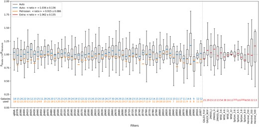
Comparison between the fluxes estimated by this pipeline and the fluxes provided in the literature. The ratios are presented as box-plots containing the 25–75 per cent percentiles, while the upper and lower limits depict the minimum and maximum ratios. The lines inside the box plots correspond to the median values for the auto, Petrosian and additional bands (blue, orange, and red coloured lines), and the legend indicates the mean value of these medians. The coloured values at the bottom of the figure display the number of galaxies that were employed to estimate the box plots for each filter.

Open in new tabDownload slide

Regarding the additional filters, a similar comparison was conducted. By exploiting the minijpas.xmatch_allwise catalogue, 10 000 randomly selected galaxies were cross-matched (adopting 5 arcsec as angular separation) with the Hermes–Herschel catalogue (Hermes et al. 2017), resulting in 1104 sources (including both extended and point-like sources). Adding the 32 galaxies under study, a number of 1135 galaxies were identified and further cross-matched with the Spitzer-SEIP catalogue (105 galaxies; Spitzer Science Center (SSC) & Infrared Science Archive (IRSA) 2021), 2MASS (74 galaxies; Cutri et al. 2003), and GALEX-AIS (30 galaxies; Bianchi et al. 2011). All the admitted flux measurements were required to satisfy the criterion of having an uncertainty that is lower than 50 per cent of its flux measurement, along with being classified as an accurate detection (e.g. photometric quality flag for WISE with a value of B or A; for more details, see Cutri et al. 2003). To note that these criteria and the relatively limited depth of all-sky surveys have led to a reduction in the number of available galaxies in the additional filters.

For all examined filters, the flux ratio between the one retrieved by the pipeline and the reference value was estimated (in the case where solely a magnitude was available from the archival catalogues, the ratio was converted by following |$\rm 10^{0.4*|m_{Breda+23}-m_{literature}|}$|⁠). Likewise the miniJPAS comparison, the results from this exercise are included in Fig. 1, with the median displayed with red colour and with a mean ratio value of 1.062. Although the herein presented is meant to exclusively analyse BCDs observed by JPAS, this exercise further supports its robustness, demonstrating its applicability to both extended and point-like sources, and rendering it qualified for the automated study of both faint and bright galaxies, both in the local and high-z Universe.

3.3 Analysis of the imaging data

The present module’s first design is to execute aperture photometry on the narrow and medium-band JPAS filters, thus extracting the photospectra from the imaging data, whereas SED extraction will be performed by the same module in later stages of the processing. Regarding the fact that the construction of both optical photospectra and SED share most of the processing stages, we decided to compile both proceedings in this subsection.

In the interest of selecting an aperture radius R_ap that encompasses virtually all of the flux emitted by our source, for miniJPAS data the adopted R_ap (pix) is equal to 1.2R_gal (arcsec) divided by the pixel scale of each individual frame F_λ. With respect to the multiwavelength data, given their lower spatial resolution as compared to JPAS, Rap is set to be twice the size of the FWHM of each individual instrument’s PSF, effectively resulting in an aperture of 4 × FWHMλ (arcsec). Regarding the sky annulus, it is defined as the area between a circle with radius R_in = R_ap + inc and a second circle with radius R_out = R_in + inc. The increment inc is adopted to be 10 pixels in all cases except for Herschel data, where it is 5, given its large pixel scale. The choice of these values has an empirical foundation, resulting from several trials adopting different values. Two masks centred in the input coordinates are created, mapping the circular area of the aperture (mask_ap) and the sky annulus (mask_sky), which will be subsequently used in the aperture photometry operation. On account of the different pixel-scales of multiwavelength data, when constructing the SED, the two previously mentioned masks will be created for each multiwavelength frame.

3.3.1 Identifying bright sources

The subsequent phase is to identify and mask all additional bright sources that may exist in each frame, this way mitigating contamination from external sources in the aperture photometry procedure. Aiming for the construction of an algorithm that operates soundly at all circumstances, this is achieved by an elaborated operation which combines several actions:

• After sky modelling and subtraction, for each individual frame create a mask comprising all bright sources (maskBS_Fλ), by detecting all excess emission brighter than 3σ as compared to the image background. This operation is performed by means of the sigma-clipping method, specifically the submodule make_source_mask from the python package photutils.

• Identify and extract contours in the mask images, thus obtaining the number, location, and dimensions of all the bright sources present in F_λ.

• Obtain maskBS_Fλ-1 by performing greyscale erosion with a square connectivity equal to one (Soille 1999) in maskBS_Fλ, this way minimizing the likelihood of our source to be merged with others (i.e. the same contour to outline our and additional sources).

• Proceed to the identification of contours in maskBS_Fλ-1 and compare it with the same obtained for the previous set of masks, prior to erosion. If the number of contours have decreased, re-apply the grey-scale erosion morphological operation to the original set of masks while adopting a structure of 2 × 2, thus avoiding neglecting sources with length in one of the spatial dimensions equal to 1 pixel.

• To avoid any risk of neglecting small-scale sources within the aperture radius, the algorithm compares maskBS_Fλ with maskBS_Fλ-1, seeking for possible contours with area of 1 pixel that were extinct after the erosion operation. If it detects any, it re-places it in maskBS_Fλ-1.

• Detect the contour corresponding to our source by identifying the one that is closer to the input coordinates and remove it from maskBS_Fλ-1.

• Perform binary dilation twice (Soille 1999) in maskBS_Fλ-1, expanding the size of each detected source, thereby obtaining the final mask of bright sources, maskBS_Fλ.

• Exclusively for multiwavelength data, having in mind the substantially broad PSF of several of the instruments here considered, it might be impossible to resolve our source if there is an external bright source in its vicinity. Towards the identification of possible nearby sources, it will estimate the distance between our source and every detected contour. Additionally, it will verify the distances of all objects listed in the SExtractor table. To redress this problem, if any of the estimated distances are lower than the PSF of the instrument, the error that will be fed to the SED fitting tools in later stages will be significantly enhanced, assumed to be 50 per cent of the measured flux within the aperture.

3.3.2 Aperture photometry

At this stage, all requirements are fulfilled to commence the aperture photometry operation, which is conducted in the following manner:

• Seclude and extract the flux of our source within the aperture (and respective sky contribution) first by multiplying each F_λ by the logical NOT (!) of maskBS_Fλ (thuswise ensuring that all bright sources within the imaging frame render 0) obtaining F_!maskBS, followed by multiplication with mask_ap. The total flux (f_ap) and number of pixels (n_ap) within the aperture are assessed by summing the flux of the image resulting from the previous operation, and by accounting for every non-zero, non-nan pixel within this area, respectively. Error estimation (σ_ap) is performed by exploiting the python submodules calc_total_error and aperture_photometry from photutils, using the individual RMS and the previously compiled exposure times. The number of valid pixels within the aperture (i.e. non-zero and non-nan) is estimated. If lower than 30 per cent of the total number of pixels within the aperture, this particular F_λ will not be considered in later stages of the processing.

• Multiply each F_!maskBS by the mask annulus mask_sky. The average flux within the annulus (μ_sky) is estimated by summing the image flux resulting from the preceding operation and subsequent division by the number of non-zero pixels within this area. In addition, the mode (Mo_sky) and the standard deviation of the sky (σ_sky) are estimated.

• The sky flux within the aperture area (f_sky) is assessed by multiplication of μ_sky by n_ap. Finally, the corrected flux radiated by our source is given by f_gal = f_ap − f_sky.

Once the SED is extracted, as a control point, the module offers visual aid as illustrated by Fig. 2 for an example source (galaxy located at RA: 214.32208°, DEC: 52.538199°). It is exhibited the various bandpasses that will be considered for this source in the SED fitting procedure, with the white circle depicting the adopted aperture whereas the black annulus indicating the area of the sky used for sky statistics. It is additionally depicted each maskBS_Fλ overlapping external bright sources. On top of each frame, it is inscribed the name of F_λ and the adopted aperture. The red ‘x’ indicates a non-detection, i.e. an upper limit for the SED fitting tools.

Figure 2.

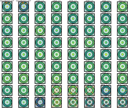
Visual output resulting from the module described in subsection 3.3 for the source located at RA: 214.32208°, DEC: 52.538199° when extracting the SED from multiwavelength imaging data. It displays all the bandpasses that will be considered in the SED fitting, with the adopted aperture overplotted in white and the sky annulus in black, in addition to the shaded areas that reflect the maskBS_Fλ. Moreover, the name of F_λ and the adopted aperture are noted on top of each frame, and the overlapped red ‘x’ on some of the panels indicates a non-detection.

Open in new tabDownload slide

3.3.3 Identifying non-detections

When considering the multiwavelength data and the subsequent SED fitting operation, it is crucial to devise a strategy for the non-supervised, accurate identification of the presence/absence of emission in the current frame. Intending to determine the criteria that are well-suited for this task, it was drafted a set of trials adopting different conditions that were later evaluated by visual inspection of an exhaustive number of individual frames. This experiment resulted in the choice of the following criteria, used for the determination of a positive detection:

1. the circle’s area, encompassing pixels brighter than Mosky + 3σsky within the aperture, should be greater than or equal to the area of a circle equivalent to the FWHM of the instrument’s PSF. In this manner, we assure that the detection (herein defined as 3σ_sky above the sky level) can be resolved by the observing telescope.

2. the fraction of the number of pixels within F_ap, which are brighter than Mo_sky + 3σ_sky must be higher than the same within f_sky, assuring that the percentage of pixels that are at least 3σ_sky above the sky level is superior within the aperture, as compared to the same within the sky annulus.

When the algorithm adjudicates a non-detection, the observed flux will be assigned to the SED fitting tools as an upper limit.

The pipeline continues by performing aperture corrections to all multiwavelength data whenever deemed necessary (i.e. when R_ap is lower enough not to encompass at least 95 per cent of the source’s luminosity, as given by SExtractor), following the recipes provided by each instrument’s handbook (see subsection 3.2 for helpful references). Error estimation for the multiwavelength data that do not provide RMS maps, such as 2MASS, is executed by adopting the prescriptions described in Cutri et al. (2003). Regarding Herschel data, as indicated by Balog et al. (2014) and Bendo et al. (2013), respectively, the flux error is of 5 per cent in all three PACS filters and 5.5 per cent in all SPIRE filters.

3.3.4 Conversion of the data units to physical units of flux

Subsequently, for each F_λ that is not in units of mJy, the measured emission f_gal is converted to physical units of flux, namely, flux density in f_λ (erg cm⁻² Å⁻¹ s⁻¹) and f_ν (erg cm⁻² Hz s⁻¹), mJy, and m_AB. This is achieved by following the prescription:

where, for each F_λ, zpt is the zero-point magnitude, AB is the AB correction factor between the Vega magnitude system, cF is the aperture correction factor and c is the speed of light in units of Å s⁻¹.

For F_λ that are in units of mJy, such as all passbands from Spitzer and Herschel, the reverse operations are applied, thus retrieving the flux in the remaining units. Both the optical photospectra and the SED in all the aforementioned flux units are stored in two fit files.

3.3.5 Detecting and assessing emission lines

After de-redshifting the extracted optical photospectra, the subsequent step consists of analysing the latter, seeking for emission lines. The procedure begins by executing the submodule find_lines_threshold from the python package, specutils, which operates by identifying deviations larger than the spectrum’s assessed uncertainty. This module was designed for the analysis of spectral data where emission lines are substantially better resolved, with its detection being therefore straightforward. In the case of low-resolution spectra such as the one obtained from miniJPAS imaging data, it is frequent for the aforementioned routine to erroneously identify emission lines. To overcome this issue, the list of detections proceeding from this python routine will be examined, being contrasted with a record of all the emission lines most commonly observed in star-forming systems, namely, Ly-α, C iv, [O ii], Mg ii, Hβ, [O iii], Hα, [N ii], and [S ii]. Provided that there are entries to which the observed wavelength differs less than 75 Å from the central wavelength of any of the well-known emission lines, it is considered a true detection.

Modelling of the detected emission lines is performed by means of the submodule RickerWavelet1D from astropy (after empirically determining that, in most cases, the latter provided better results as compared to a Gaussian fit), thus obtaining the mean (central wavelength) and standard deviation (broadness) for each emission line that was previously detected. The continuum in the vicinity of the emission line is estimated by fitting a second-degree polynomial to the photospectra, deprived of all deviant points (defined as being lower/higher than the average flux minus/plus its estimated standard deviation). Fluxes and EWs are determined by means of the specutils submodules line_flux and equivalent_width, respectively, applied in the spectral region between the previously estimated central wavelength of each detected emission line minus/plus its standard deviation. After conducting several tests to establish the threshold of detectability, the empirical limit of 25 Å was selected as the minimum acceptable equivalent width (EW) (note that the narrow bands from JPAS partly overlap, hindering any exact assessment of fluxes and EWs of emission lines). If the detected emission line is listed in the cigale default filters, its integrated flux will be taken into account in the SED fitting operation (the poor precision of the measured fluxes should not obstruct the SED fitting procedure, considering that cigale does not require exact measurements but merely their order of magnitude). An illustrative example is given by Fig. 3, which displays the visual output generated by this module for one of the processed galaxies. It is displayed the RGB image in the left-hand-side with the adopted aperture overplotted in white and the restframe photospectra in the right-hand-side, where it is highlighted the detected emission line (most probably resulting from the sum of [O iii]₄₉₅₉ and [O iii]₅₀₀₇), with an estimated EW of 592 Å). The light-blue dashed line depicts the fit to the emission line and the purple dashed line the estimated continuum utilized for the determination of the line EW.

Figure 3.

Visual output resulting from the module outlined in subsection 3.3.5. In the left-hand-side, it displays the RGB image of the source with the adopted aperture overplotted in white, and in the right-hand-side, it exhibits the rest-frame optical photospectra obtained for the source located at RA: 214.32208°, DEC: 52.538199° (and its respective spline interpolation in grey), along with the [O iii] emission line outlined by the light-blue dashed line. The determined continuum is depicted by the purple dashed line. The shaded light-blue area highlights the region where the emission line was identified.

Open in new tabDownload slide

3.3.6 Executing cigale

At this stage, the present module initiates the execution of an additional module that addresses the creation of the cigale input files and subsequent execution. For the sake of completeness, we provide a brief description of the necessary files: the cigale data file must contain one row with the galaxy ID, adopted redshift, and the flux values in units of mJy. The model configuration file (pcigale.ini) will define cigale’s context, encoding the characteristics of the data (namely the passbands to which the values in the data file correspond) and of the models that will be generated to fit the observational data. By default, it is assumed to have a Salpeter IMF (Salpeter 1955) and a delayed star-formation history (SFH) with an optional exponential burst. Note that originally cigale did not have the JPAS filter scheme installed. This operation must be previously performed independently (see Burgarella, Buat & Iglesias-Páramo 2005, for detailed information on cigale and how to prepare and execute it).

As a control point, an additional illustration is produced (Fig. 4), displaying the observed SED to be fitted by cigale and Prospector, subsequently. It indicates the spectral regions of the various pass bands, colour coded from blue to red by increasing wavelength, and the emission lines that were detected in grey. The observational points are displayed in black if considered detections and dark red if deemed non-detections by the technique elaborated in subsection 3.3.3.

Figure 4.

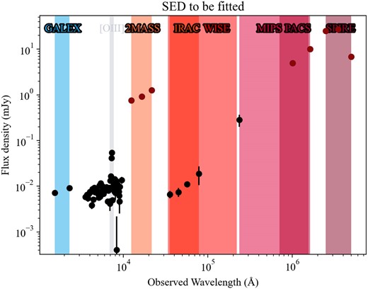
Illustration of the observed SED prior to fitting for the sample galaxy displayed in previous figures, with the x-axis in logarithmic units and the y-axis in units of mJy. The spectral regions of the different passbands are shown, with colours ranging blue to red, and the field points are colour coded according to a detection (black) or non-detection (dark-red). It is additionally highlighted in grey in the region where the emission line was detected.

Open in new tabDownload slide

Once cigale’s operation is complete, the previously introduced module 3.3 generates a graphical output of the resulting fit, additionally displaying some of the obtained physical properties, as apparent from inspection of the left-hand side of Fig. 5. The latter displays the best-fit SED model retrieved by cigale and the observational points and the upper limits in black and red, respectively.

Figure 5.

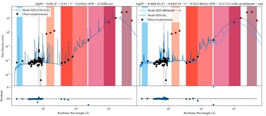
Visual output illustrating the SED fitting results by cigale (left-hand side) and Prospector (right-hand side) for the same exemplar. Both the flux density (in units of 1e⁻¹⁷ erg cm⁻² s Å) and the restframe wavelength (Å) are displayed in a logarithmic scale. The best-fitting SED models are represented by solid blue lines, the observational points by the black points and the upper limits by the dark red points. The residuals are shown in the low panel, and some of the derived physical properties are shown in the image title.

Open in new tabDownload slide

3.3.7 Executing prospector

The module accountable for the execution of Prospector starts by assembling the two models for inference and implementing a parametric (delayed-τ) and a non-parametric (α, Leja et al. 2017) star-formation history (SFH). The model referring to the parametric SFH was constructed by selecting the default parametric SFH from Prospector template library with a log uniform mass prior and adding the models for both dust and nebular emission (see Prospector user guide for a comprehensive description of the provided models). With regard to Prospector-α, it includes dust attenuation and re-radiation, a flexible attenuation curve, nebular emission, stellar metallicity, and a non-parametric SFH with six components. The simple stellar population (SSP) library is produced according to the adopted SFH. In addition, nebular emission and dust (and AGN, if the object was previously classified as QSO) contributions are included. The redshift is fixed, and it has adopted a Salpeter IMF. The dictionary encompassing the observational data is assembled, which comprises the list of the utilized passbands, the evaluated fluxes and respective uncertainties in each filter in maggies units, and the effective wavelength for each of the filters. The subsequent step is to optimize the parameters of the calibration functions for each generated model. The posterior probability distribution is estimated by sampling, either through an affine-transform-invariant version of Metropolis-Hastings MCMC (emcee) or nested sampling (dynesty). Hereupon, the SED is fitted and the results are stored. Similarly as the cigale module, a graphical output is produced, summarizing the obtained physical properties for both models (such as present-day stellar mass (M_⋆), mass-weighted mean stellar age (t_M) and metallicity (Z_M), and SFRs), and displaying the resulting best-fitting models, as exemplified by the right-hand side of Fig. 5.

3.3.8 Estimate restframe SDSS colours and magnitudes, fluxes, and luminosities for each bandpass

Subsequently, restframe magnitudes, fluxes, and luminosities, along with intrinsic colours and apparent and absolute magnitudes in the SDSS filters i, g, and r are estimated. Such is accomplished by convolving each of the filter transmission curves T(λ) with the restframe SED, as subsequently clarified.

Primarily, the restframe best-fitting SED is interpolated to the step of each T(λ), followed by its normalization, so that the sum of its flux density is equal to one, resulting in sp(λ). Subsequently, to obtain the flux in each bandpass f|$\rm _{F_{\lambda }}$| in units of f_λ (erg cm⁻² Å⁻¹ s⁻¹), it is applied the successive equation:

Conversion to f_ν units (erg cm⁻² Hz s⁻¹) is performed by multiplying f|$_{\rm F_{\lambda }}$| by |$\lambda _{\rm eff}^2$|/c × 1e10²³, obtaining f|$\rm \nu _{F_{\lambda }}$|⁠, which in turn is converted to apparent and absolute magnitudes¹⁰ (m/M) through:

where D is the galaxy distance in units of Mpc. Restframe SDSS colours are estimated through:

Finally, restframe luminosities within each bandpass L|$_{\rm F_{\lambda }}$| are estimated by:

where R is equal to D in units of cm.

4 EXPLORATION OF THE PHYSICAL PROPERTIES OF THE MINIJPAS EELGS

The coordinates of the 31 extreme line emitters identified by the IP22 algorithm (20 EELGs and 11 QSOs) in the miniJPAS data were provided to the pipeline described in the previous section. In this fashion, their multiwavelength photometry was retrieved and analysed by both cigale and Prospector (delayed-τ and α SFH models), thus obtaining stellar mass, mass-weighted stellar age estimates, SFRs, AGN fractions, etc.. In addition, by convolving the resulting SED with the filter transmission curves of each instrument, we retrieved absolute magnitudes and colours. The collected results were contrasted with the physical properties of a reference sample of ∼500 EELGs, as obtained by processing their SDSS optical spectra with fado (Gomes & Papaderos 2017), as provided by Breda et al. (2022).

Certain galactic properties assessed by the various SED fitting operations here probed are displayed in Fig. 6, which illustrates, from left to right, the estimates for the stellar mass, SFRs, mass-weighted mean stellar age, and metallicity. The solid line represents the equality line, and the dashed lines denote the mean dispersion of the differences between the estimates obtained for each model. Inspection of this figure evidences that the stellar mass and the SFRs are fairly consistent (the mean σ of the differences between models is of 0.5 dex for the stellar mass estimates and of 0.35 M_⊙ yr⁻¹ for the SFR), although Prospector delayed-τ tends to provide lower stellar mass underestimates. Nevertheless, it is evident that, as expected, QSOs register rather higher differences as compared with the EELGs. Regarding the stellar properties, the mass-weighted mean stellar ages display a higher degree of variation, with an average dispersion of 0.73 dex, whereas the mass-weighted mean stellar metallicities exhibit a mild degree of inconsistency between the three sets of estimates (with their differences displaying an average σ of 0.16 Z_⊙). Such result is also observed in previous works using state-of-the-art spectral synthesis techniques, which are the most reliable method available for the characterization of stellar populations in galaxies (e.g. Breda et al. 2022, and references within).

Figure 6.

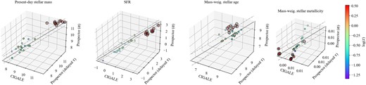
A visual representation of the estimates of the present-day stellar mass, SFR, mass-weighted stellar age, and metallicity (from left to right) for the three models for the sample galaxies. Data points (EELGs and QSOs) are colour coded according to the logarithm of their redshift, and QSOs are encircled within larger, empty circles. The solid line represents unity and the dashed lines the average dispersion (1σ).

Open in new tabDownload slide

Fig. 7 illustrates the stellar mass estimates versus the absolute magnitude in the three SDSS bands g, r, and i, as obtained by both SED fitting tools, simultaneously while contrasting with the same for the reference EELG sample. Generally, it is observed a sound agreement between the EELGs here in the study and the reference sample, with the results by cigale and Prospector-α displaying higher coherency and lower levels of dispersion. In contrast, stellar masses recovered by Prospector delayed-τ tend to be systematically lower for the respective intrinsic magnitudes as compared to the reference sample, being in average 0.42 dex lower as compared to the stellar masses recovered by cigale. These findings are remarkably consistent with previous results. In Lower et al. (2020), the authors compare the derived galaxy properties obtained by SED fitting, by assuming a parametric and a non-parametric model, for a set of ∼1600 mock galaxies from the SIMBA cosmological simulation (Davé et al. 2019), with stellar masses ranging from 4.4|$\times 10\rm ^{7}$| to 1.4|$\times 10\rm ^{12}$|⁠. As illustrated by their Fig. 3, these authors report that the estimated stellar masses assuming the Prospector delayed-τ model were, on average, approximately ∼0.4 dex lower than the true stellar mass. In contrast, the Prospector-α model recovers more accurately the true stellar masses within their sample. Regarding the QSOs, as expected, these are located at the high mass vs. high magnitude locus, yet following the same extrapolated trend for the SDSS EELG sample, demonstrating that the stellar mass estimates obtained for the EELGs and QSOs identified in miniJPAS are sound. An additional test was conducted by running the sample exclusively using optical JPAS data. Such resulted in a systematically higher SFR (∼0.42 dex, in average), with no significant variation in the remaining parameters. This result is not surprising, considering that the FIR photometry, which constrains the dust temperature, is tightly correlated with the level of SFR (the FIR photometric points, or upper limits in most cases, compel the solution to converge to lower dust temperatures, implying lower SFRs).

Figure 7.

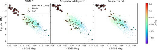
Absolute magnitude in the r SDSS optical band versus the estimated present-day stellar mass M_⋆ as obtained by cigale (left-hand side column), Prospector delayed-τ (central column), and Prospector-α (right-hand side column). Analogously to Fig. 6, data points are colour-coded according to the logarithm of their redshift, and QSOs are encircled within larger, empty circles. The transparent points represent the reference EELG sample.

Open in new tabDownload slide

An additional test was conducted by running the sample exclusively using optical JPAS data. The obtained results remained consistent with those derived from utilizing the complete set of available photometric data, showing slightly higher SFRs.

The stellar surface density was computed by dividing the obtained stellar mass estimates by the projected area (i.e. Σ_⋆ = M_⋆/π |$R_{\rm gal}^{2}$|⁠). The relations between the logarithm of Σ_⋆ and the estimated logarithm of the mass-weighted stellar age is shown in Fig. 8 for the three SED fitting operations (from left to right, cigale, Prospector delayed-τ, and Prospector-α). Although, there are severe differences between the mass-weighted stellar age estimates as given by the three SED fitting procedures, they all roughly follow the reference correlation.

Figure 8.

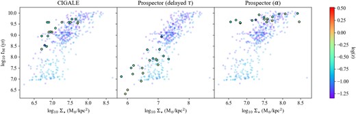
Relation between the logarithm of the stellar surface density Σ_⋆ and the logarithm of the estimated mass-weighted stellar age t_M as obtained for the three SED fitting operations and contrasted with the same for the reference sample.

Open in new tabDownload slide

Finally, the top panels of Fig. 9 illustrate the logarithm of the present-day stellar mass M_⋆ versus the logarithm of the specific star formation rate sSFR (i.e. the SFR divided by the estimated stellar mass), whereas the bottom panels display the relation between the estimated mass-weighted mean stellar age t_M and the logarithm of the sSFR for the three SED fitting procedures.

Figure 9.

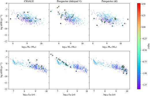
The top panels illustrate the logarithm of the present-day stellar mass M_⋆ versus the logarithm of the specific star formation rate sSFR, i.e. the SFR over the estimated stellar mass. The bottom panels display the logarithm of the mass-weighted stellar age t_M versus the logarithm of the specific star formation rate. The three panels display the respective results for each of the three SED fitting operations (from left to right, cigale, Prospector delayed-τ, and Prospector-α).

Open in new tabDownload slide

Comparison between the three SED fitting operations indicates that the obtained results are consistent with the reference correlations. Nevertheless, although the stellar mass estimates and sSFRs are fairly coherent between models, the parametric model (Prospector delayed-τ) tends to underestimate the total stellar mass as compared to the remaining determinations, as previously noted by Leja et al. (2019a, 2019b, 2020). Regarding mass-weighted stellar ages and metallicities, these display a higher level of variance. As clearly shown by the middle panel of the bottom row of Fig. 9, mean stellar ages recovered by Prospector delayed-τ tightly correlate with the sSFR. Such a result is expected considering that stellar ages are a direct function of the SFH (i.e. the adopted τ), being analytically computed from the assumed SFH, contrasting with the Dirichlet SFH prior (Prospector-α) which only weakly couples the SFR to the earlier SFH (Leja et al. 2017, 2018). This outcome reinforces the notion that parametric methods are over-simplistic and incapable of realistically recovering the complex SFHs of galaxies as the EELGs studied herein (e.g. Lower et al. 2020). Inspection of this panel additionally reveals an inconsistency between the theoretical prediction and observations, strongly suggesting that an exponentially delayed SFH with a specific τ is oversimplistic, being unable to appropriately describe the SFH of EELGs, which are expected to be considerably more complex. On the other hand, the mean stellar ages estimated by Prospector-α tend to accumulate at the high end of the parameter space. For the lower-mass galaxies, the mass-weighted stellar age given by this model appears overestimated as compared to the reference sample, as reflected by the third panel of Fig. 8.

Besides the registered inconsistencies, mainly in stellar ages and metallicities, overall the obtained relations indicate that the developed pipeline produces physically reasonable results and is an appropriate tool for the automatic multiwavelength analysis and assessment of the main properties of galaxies that lack spectroscopic information.

5 SUMMARY AND CONCLUSIONS

The present work describes the development of a fully automated, modular pipeline with the main purpose of the characterization of galaxies with absent spectroscopic information, through a multiwavelength exploration. The pipeline, scripted in the python programming language, fully open access and offered to the community via the repository GitHub, requires only the coordinates of the desired object.

It commences by retrieving the available photometric information of the source by seeking in several repositories, namely in the miniJPAS, MAST, and IRSA-IPAC data bases, and collecting photometric data from GALEX, JPAS, 2MASS, WISE, Spitzer, and Herschel, and the respective RMS maps, when available. Subsequently, and after masking all bright sources apart from the one under study, it performs aperture photometry in all available passbands, with adapted apertures according to the optical radial extent of the object and the respective FWHM of each instrument. It follows by identifying non-detections, which will be interpreted as upper limits in the SED fitting operations while constructing the observed SED. Additionally, the pipeline detects and assesses emission lines in the optical data, whose integrated fluxes will be used as input in the SED fitting with cigale. Finally, it initiates the SED fitting procedures by means of two distinct SED fitting tools (cigale and Prospector), for three individual models.

This strategy, contrary to retrieving data from the available catalogues with fixed apertures, assures consistency and homogeneity throughout the whole set of multiwavelength data, which is particularly important, specially in light of the faint nature of these objects. The obtained results are in overall agreement with previously known relations derived from detailed spectral synthesis of a sample of ∼500 EELGs from SDSS, reassuring reliability of the developed method. In addition, the soundness of the retrieved photometry was assessed, revealing solid agreement between the reference values, and demonstrating that the herein developed pipeline is suitable for the automated study of bright and faint sources, point-like or extended, and at local or high-z.

While EELGs are infrequent in our nearby cosmic neighbourhood, their study holds great significance, since these serve as valuable counterparts within our local environment mirroring the characteristics of star-forming galaxies from the early Universe, similar to those newly uncovered by the JWST, e.g. Withers et al. 2023. This work serves as a proof of concept, demonstrating the reliability of the developed pipeline and paving the way for attaining massive and automated characterization of the EELGs that will be soon detected within the ∼8000 deg² of the northern sky covered by JPAS.

ACKNOWLEDGEMENTS

IB, JVM, JIP, CK, EPM, AAP, and RGD acknowledge financial support from the State Agency for Research of the Spanish MCIU through the ‘Center of Excellence Severo Ochoa’ award to the Instituto de Astrofísica de Andalucía (SEV-2017-0709). JVM, JIP, CK, and EPM acknowledge financial support from projects Estallidos7 PID2019-107408GB-C44 (Spanish Ministerio de Ciencia e Innovacion), and grant P18-FR-2664 (Junta de Andalucía). RGD and LADG acknowledge financial support from the State Agency for Research of the Spanish MCIU through ‘Center of Excellence Severo Ochoa’ award to the Instituto de Astrofísica de Andalucía (SEV-2017-0709) and CEX2021-001131-S funded by MCIN/AEI/10.13039/501100011033. LADG, RMGD, RGB, GMS, and JERM are also grateful for financial support from the projects PID-2019-109067-GB100 and PID2022-141755NB-I00.

Based on observations made with the JST250 telescope and PathFinder camera for the miniJPAS project at the Observatorio Astrofísico de Javalambre (OAJ), in Teruel, owned, managed, and operated by the Centro de Estudios de Física del Cosmos de Aragón (CEFCA). We acknowledge the OAJ Data Processing and Archiving Unit (UPAD) for reducing and calibrating the OAJ data used in this work.

Funding for OAJ, UPAD, and CEFCA has been provided by the Governments of Spain and Aragón through the Fondo de Inversiones de Teruel; the Aragonese Government through the Research Groups E96, E103, E16_17R, and E16_20R; the Spanish Ministry of Science, Innovation and Universities (MCIU/AEI/FEDER, UE) with grant PGC2018-097585-B-C21; the Spanish Ministry of Economy and Competitiveness (MINECO/FEDER, UE) under AYA2015-66211-C2-1-P, AYA2015-66211-C2-2, AYA2012-30789, and ICTS-2009-14; and European FEDER funding (FCDD10-4E-867, FCDD13-4E-2685).

DATA AVAILABILITY

The data underlying this article are publicly available in the miniJPAS archive, at https://www.j-pas.org/datareleases/minijpas_public_data_release_pdr201912.

Footnotes

References