


ABSTRACT
The statistical technique ‘Complex Demodulation’ (CDM) is used to track the amplitude and phase changes of periodicities in five naked T Tauri stars. The periodicities are most likely caused by dark spots on the stellar surfaces, which are rotated into and out of view. Two of the stars (CD-56 1438, CD-72 248) show two independent periodicities, probably due to being binary weak-lined T Tauri stars. Two different low-pass filters, operating, respectively, in the frequency and time domains, are used as part of the CDM methodology. Statistical aspects of the estimated amplitudes and phases are investigated in some detail: in particular, expressions are derived for standard errors and for possible biases. A large variety of different types of amplitude and phase changes are found, including approximately linear or quadratic, abrupt level shifts, pulses, and oscillatory. Long term changes in amplitudes are aperiodic, but mimic long-term cycles.
1 INTRODUCTION
Low-mass (M < 2 M⊙) pre-main sequence (PMS) stars can be subdivided into two groups: classical T Tauri stars (CCTSs) and weak-lined T Tauri stars (WTTSs). Although there is some overlap, CTTSs are roughly younger than about 4 Myr, while ages of WTTSs are in the range 4–10 Myr. The former group of stars is characterized by the presence of circumstellar discs [Lada (1987) Young Stellar Object (YSO) class II], and typically exhibit photometric variability caused by accretion and/or variable extinction. A comprehensive review of CTTS variability types (FU Ori, UX Lup, ‘bursters’, ‘dippers’, UX Ori, RW Aur, etc.) can be found in Fischer et al. (2023); these differ in the amplitudes, durations, and aperiodic light curve shapes. In addition, flaring events associated with magnetic fields, and periodic brightness modulation due to star-spots are also observed.
WTTSs, which belong to YSO class III, have lost most or all of their circumstellar material (e.g. Padgett 2006; Wahhaj et al. 2010). Consequently, their variability is typically much simpler, being induced by star-spots on the stellar surface that rotate in and out of view (e.g. Wang et al. 2023). Aside from these periodic brightness changes, some WTTS also show magnetic flares. Amplitudes of the periodic variations are typically a few tenths of a magnitude in the V-band, but could be as low as a few per cent of the flux (e.g. Grankin et al. 2008). Periods of the stars range from a few hours to several days (e.g. Affer et al. 2013; Karim et al. 2016; Rebull et al. 2022).
Long continuous time series of WTTSs have been obtained by a number of satellite missions – MOST (Walker et al. 2003 – see e.g. Rucinski et al. 2008; Siwak et al. 2011; Cody et al. 2013); CoRoT (Auvergne et al. 2009 – see e.g. Affer et al. 2013; Lanza et al. 2016); Kepler/K2 (Borucki et al. 2010; Howell et al. 2014 – see e.g. Hambálek et al. 2019; Stauffer et al. 2017, 2021); and TESS (Ricker et al. 2015 – see e.g. Rebull et al. 2022).
Koen (2015) presented ground-based multifilter photometry of four short period (P < 1 d) weak-lined T Tauri stars (WTTSs), obtained over 4–5 nights for each star. He noted that the observed photometric variability could be explained by cool star-spots on the stellar surfaces, and estimated spot temperatures and filling factors from the relative amplitudes seen in the different filters. Interestingly, variability amplitudes were seen to change dramatically over time-scales of 1–2 d.
This paper is by way of an updated view of the variability in the stars, benefitting from the availability of uninterrupted space-based observations by the ‘Transiting Exoplanet Survey Satellite’ (TESS – Ricker et al. 2015). A fifth star – CD-56 1438 – is added to the four objects studied by Koen (2015). All five stars are members of young associations: Columba (CD-36 3202); Argus (CD-49 1902, CD-56 1438); and Octans (CD-66 395, CD-72 248) (e.g. Da Silva 2009).
Some basic information about the five stars is presented in Table 1. Three periods are listed: P1 is from Kiraga (2012), who used ‘All Sky Automated Survey’ (ASAS – Pojmanski 1997) photometry to find periodicities in bright X-ray sources. The second set of periods P2 were extracted from the TESS observations. Being densely sampled, these measurements could be used to gain a more precise picture of the frequency content of the variability; for example, CD-56 1438 and CD-72 248 clearly have more than one independent frequency. Analysis of the TESS data therefore allowed the ASAS data, with its long time baseline of 9 yr, to be revisited in order to derive periods P3 with good accuracy. Periods P2 are used in the analysis below; there is little difference between these and P3, except for the case of CD-49 1902.
Information about the target stars. Spectral types are from Torres et al. (2006) and rotational velocities from Zúñiga-Fernández et al. (2021) (except for CD-49 1902, for which vsin i is from Torres et al. 2006). The radial velocity ranges and number n of measurements of Vr are from the Simbad data base.1 The original sources are Torres et al. (2006), Gaia Collaboration (2018), Steinmetz et al. (2020), Jonsson et al. (2020), and Zúñiga-Fernández et al. (2021). Periods in columns 6–8 are from Kiraga (2012) (based on ASAS photometry); analysis of TESS data in this paper; and a re-analysis of the ASAS data.
| Name | Spectrum | vsin i | Vr range | n | P1 | P2 | P3 |
|---|---|---|---|---|---|---|---|
| km s−1) | km s−1 | (d) | (d) | (d) | |||
| CD-36 3202 | K2Ve | 52 (3) | (16, 27) | 3 | 0.23533 | 0.2353 | 0.23526 |
| CD-49 1902 | G7V | 55 (5.5) | (19, 20) | 2 | 0.90750 | 0.9023 | 0.90756 |
| CD-56 1438 | K0V | 62 (3) | (13, 27) | 3 | 0.41848 | 0.1997, 0.4184 | 0.19964, 0.41833 |
| CD-66 395 | K0IV | 60 (5) | (8, 17) | 3 | 0.21280 | 0.2710 | 0.27099 |
| CD-72 248 | K0IV | 62 (0.5) | (−34, 13) | 5 | 0.235576 | 0.2356, 0.2514 | 0.23558, 0.25138 |
Luminosities of the stars can be calculated by using published photometric measurements conveniently available from the VizieR service2 of the Strasbourg astronomical Data Center. Original sources of the data are APASS (‘AAVSO Photometric All-Sky Survey’; Henden et al. 2015), Gaia (Gaia collaboration 2021), the ‘SkyMapper Southern Survey’ (Wolf et al. 2018), 2MASS (‘Two Micron All-Sky Survey’, Skrutskie et al. 2006), and WISE (‘Wide-field Infrared Survey Explorer’, Wright et al. 2010). The efforts of these surveys are gratefully acknowledged. Assuming preliminary values for the effective temperature of each star, bolometric corrections (Choi et al. 2016) can be obtained by interpolation in the ‘MESA Isochrones and Stellar Tracks’ tables.3 Results are not sensitive to gravity, hence a fixed value of log g = 4 is assumed for each of the stars. Combining the corrected magnitudes with parallaxes (Gaia Collaboration 2021) leads to a set of bolometric magnitudes. The assumed temperature can then be adjusted to minimize the scatter in the set of bolometric magnitudes. We note that all five stars show 0.1–0.2 mag excesses at the shortest (SkyMapper u and v) and longest (WISE W1, W2, and W3) wavelengths. The excess blue emission is probably due to chromospheric activity (e.g. Ingleby et al. 2013), while the infrared excesses could be ascribed to circumstellar material (e.g. Cieza et al. 2007).
The results are in Table 2. For comparison, the effective temperatures expected on the basis of the spectral types in Table 1 are also listed; note that these values of Teff are appropriate for PMS stars (Pecaut & Mamajek 2013). Two sets of estimated temperatures are listed; those in column 3 of the table exclude the two shortest wavelength magnitudes. Values of Mbol were also calculated excluding u and v; including these lead to results which are at most 0.04 mag brighter. Given the PMS nature of the stars it is no surprise that the bolometric magnitudes are larger than those of main sequence dwarfs of the same spectral types (Pecaut, Mamajek & Bubar 2012; Pecaut & Mamajek 2013).
Properties derived from photometric measurements and parallaxes of the stars. The second column contains effective temperatures derived from all available standardized photometry. The third column temperatures are based on photometry exluding SkyMapper u and v. For comparison, temperatures in the fourth column are those expected from the MS spectral types (Pecaut & Mamajek 2013). Errors on Mbol are given in brackets. Bolometric magnitudes in column 6 are given for comparison: these are for main sequence dwarfs of the same spectral types.4 The last column shows the maximum number of photometric filters taken into account.
| Name | Teff, 1 | Teff, 2 | Sp. Teff | Mbol | Dwarf Mbol | n |
|---|---|---|---|---|---|---|
| (K) | (K) | (mag) | (mag) | |||
| CD-36 3202 | 4900 | 4820 | 4760 | 5.94(0.02) | 5.02 | 20 |
| CD-49 1902 | 5430 | 5310 | 5290 | 5.07(0.02) | 5.88 | 16 |
| CD-56 1438 | 5190 | 5070 | 5030 | 4.81(0.04) | 5.54 | 20 |
| CD-66 395 | 5470 | 5310 | 5030 | 4.99(0.02) | 5.54 | 19 |
| CD-72 248 | 5040 | 4870 | 5030 | 4.84(0.03) | 5.54 | 18 |
The primary aim of this paper is the detailed investigation of amplitude and phase changes in the fundamental frequencies of variability of the five stars. The next section of the paper motivates the study and describes preparation of the data for analysis. The mathematical technique to be used for the purpose, complex demodulation (CDM), is discussed in detail in Section 3. Particular attention is paid to the topics of bias and errors in the estimates, as this information appears to be absent from the literature. Results are given in Section 4, followed by a discussion of binarity (Section 5) and concluding remarks in Section 6.
Times of observation are conveniently given as
where JD is the conventional Julian Date. Also for convenience, starnames will be abbreviated in what follows, retaining only ‘CD’ followed by the first two digits (e.g. CD-36 3202 becomes CD36).
2 TESS DATA
TESS ‘Pre-search data conditioned simple aperture photometry’ (PDCSAP) of the stars was download via the ‘Mikulski Archive for Space Telescopes’.5 A summary of the data content is given in Table 3.
Pertinent information about the TESS observations of the five stars.
| Name | Sectors | Interval covered | Cadence | Range N | |$\overline{N}$| |
|---|---|---|---|---|---|
| (TJD) | (min) | ||||
| CD-36 3202 | 6–7 | 1468.27–1516.09 | 2 | 6300-8508 | 7778 |
| 33–34 | 2201.74–2254.06 | 10 | 1677-1747 | 1719 | |
| CD-49 1902 | 5–7 | 1438.14–1516.07 | 30 | 418-576 | 536 |
| 31–33 | 2144.53–2227.57 | 10 | 1596-1854 | 1711 | |
| CD-56 1438 | 4–12 | 1410.91–1652.89 | 2 | 4871-9977 | 7839 |
| 27–32 | 2036.28–2200.03 | 2 | – | – | |
| 34–39 | 2229.16–2389.72 | 2 | – | – | |
| CD-66 395 | 8–13 | 1517.92–1682.36 | 2 | 5025-9936 | 7920 |
| 27–35 | 2036.28–2279.97 | 2 | – | – | |
| 37–39 | 2308.37–2389.70 | 2 | – | – | |
| CD-72 248 | 1–13 | 1325.31–1682.32 | 2 | 4824-10027 | 8073 |
| 27–39 | 2036.28–2389.72 | 2 | – | – |
The analysis which follows is applied to individual TESS orbits, rather than sectors, since the CDM method requires data to be regularly spaced. The mean gap between successive orbits within a sector is 2.8 d, with a mean orbit duration of 11 d.
Fig. 1 shows the most interesting parts of amplitude spectra of the photometry of CD49. Examination of the figures shows very obvious changes in the amplitudes of both dominant frequencies and harmonics. Note, for example, the dramatic decrease in the amplitude of variability in CD49 from sectors 5 to 6. Also, in the sector 31 photometry of this star, the first harmonic amplitude is slightly larger than that of the fundamental, while by the end of sector 33, the harmonic has virtually disappeared.
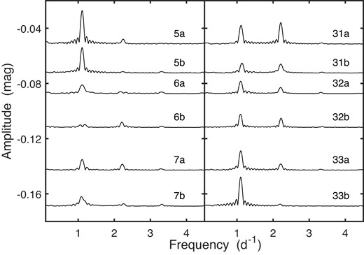
Amplitude spectra of the TESS photometry of CD-49 1902. Individual spectra are labelled with their sector numbers, and with ‘a’ or ‘b’, denoting, respectively, the first and second orbits.
The somewhat peculiar-looking double-peaked feature in the spectra of CD56 near frequency 5 d−1 is perhaps worth remarking on (Fig. 2): one of the peaks is the first harmonic of f = 2.390 at 4.780 d−1, the other is an independent periodicity with a fundamental frequency 5.008 d−1. Similarly, in the spectra of CD72 (Fig. 3), two closely spaced independent fundamental frequencies (at 3.979 and 4.245 d−1) are visible. Interestingly, in this star, variability with the lower of the frequencies is much less prominent during the second season of observations (particularly sectors 27–28 and 35–39). Other amplitude spectra are in the supplementary material.
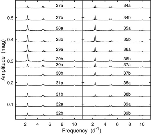
As for Fig. 1, but for the second season of TESS observations of CD-56 1438.
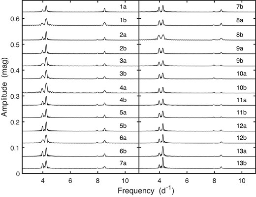
As for Fig. 1, but for the first season of TESS observations of CD-72 248.
The rest of this section of the paper is devoted to a description of the necessary pre-processing of the data needed in order to mitigate the effects of outlying observations, which are mostly the results of microflares. The situation is illustrated by Fig. 4, the top panel of which shows the sector 29a light curve of CD66. Residuals left after pre-whitening by the fundamental frequency of variation and its first few harmonics are plotted in the middle panel. Small flares near TJD 2090, 2096, and 2097 are visible. With the benefit of hindsight, these can also be seen in the original light curve. It is also evident that some care needs to be taken in any automated procedure for outlier detection, as the trend visible in the residual plot could shift acceptable datapoints to unacceptable levels (and vice versa). The residuals graphed in the middle panel were therefore subjected to further rounds of pre-whitening, this time by low (f < 0.9 d−1) frequencies. The results are plotted in the bottom panel. Note also that the limits defining outliers (shown by the two parallel lines in the bottom panel) need to be set quite generously, for two reasons: first, the rather obvious amplitude change visible in the top panel translates into considerable residual fluctuations in the bottom panel, which are not related to outliers. Second, although for a single zero-mean Gaussian the probability of observing a value outside the ±3.5σ limits is only 0.05 per cent, in the present case 7454 residuals are being considered, greatly enhancing the probability of a seeing spuriously large (or small) values.
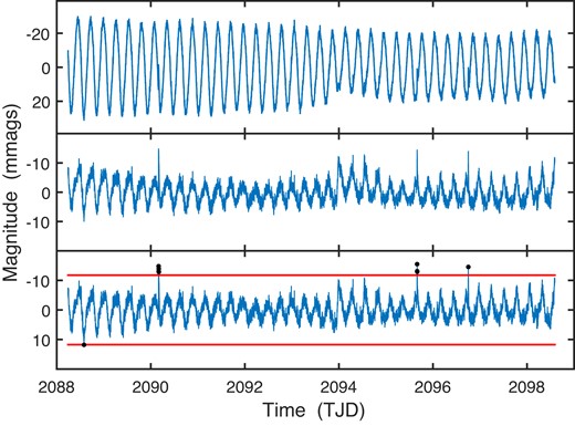
Top panel: the sector 29a light curve of CD-66 3202. Middle panel: residuals after prewhitening by the fundamental frequency (3.69 d−1) and its first three harmonics. Bottom panel: residuals after further prewhitening by low frequencies to remove trends. The (red) lines are at ±3.5σ. Black dots mark the nine residuals exceeding the limits.
Outliers detected in this manner are dealt with by replacing them by more typical values, estimated by linear interpolation. The few missing values in the downloaded photometry are similarly filled in by linear interpolation, as the demodulation technique requires observations to be spaced regularly in time.
For extended flares linear interpolation over the affected section of the light curve may fall short, particularly if the light curve shape is complex. This is so because the linear replacement section will mimic an abrupt change in the light curve properties. It is noteworthy that three of the stars – CD56, CD66, and CD72 – have been identified by Tu et al. (2020) as giving rise to ‘superflares’ (energy exceeding 1033 erg, duration longer than 1 h). The solution implemented is as follows:
Manually identify large extended flares, and note the start and end points t1 and t2 of the light curve section to be replaced.
Use the preceding cycle [y(t1 − P), y(t1)] of the light curve as a template for the replacement (P being the dominant period of variability).
- Setand interpolate u(t) in the points tj which cover the flare.$$\begin{eqnarray} u(t)=y(t-P),{\qquad}t_1 \le t \le t_2, \end{eqnarray}$$
A few examples can be seen in Fig. 5.
Examples of large flares that could not be replaced by linearly interpolated values. Instead, the preceding cycle of variability was used to reconstruct (black plus signs) the normal light curve shape underlying the flare. From top to bottom: CD-36 3202 sector 7b; CD-36 3202 sector 34b; CD-66 395 sector 11a. The latter is identified as a ‘superflare’ by Tu et al. (2020).
Finally, features that are not of interest are pre-whitened from the photometry before demodulation, to avoid spectral leakage. These include harmonics of the frequency of interest, unwanted independent frequencies (in the cases of CD56 and CD72) and their harmonics, and possible low frequency (<1 d−1) trends. Note that for CD56 and CD72, separate analyses are carried out for the two principal independent frequencies.
3 COMPLEX DEMODULATION
Complex demodulation is a time domain method used to identify trends in the amplitude and/or phase of sinusoidally varying time series (e.g. Bloomfield 2000). For the convenience of the reader a brief introduction follows.
The model is
where the amplitude A and the phase Φ may be slowly varying functions of time, and e accounts for random variability superimposed on the sinusoidal signal. Of course, in practice, the frequency ω0 = 2πf0, which is here assumed fixed, may also be variable. However, formally, only changes in the argument ω0t + Φ can be detected. We speculate that in the context of star-spots phase changes, as induced by changes in spot sizes or longitudinal drift, may be more prominent than frequency changes due to latitudinal drift to surface regions with different rotation velocities. Phase changes are easier to model, and that is what is done here, with the caveat that frequency changes may be present.
In order to introduce CDM note that (1) is equivalent to
Multiply through by exp (−iω0t) to find
If it is assumed that the changes in A and Φ are slow compared with the time-scale P = 2π/ω0 of rotation, then the first term on the right-hand side of (2) is dominated by low frequencies, while the other two terms vary more rapidly with frequencies 2ω and ω. The implication is that low pass filtering can be used to dampen the high frequency terms and to extract
where the tilde indicates the result of the filtering. It follows that
where Yi and Yr are, respectively, the imaginary and real parts of the function Y.
It may appear paradoxical that low-pass filtering is now being used to estimate the low-frequency feature Y(t), when low-frequency components of the data were removed when pre-processing the TESS photometry as described in section 2. However, these are quite distinct components of the time series: in (1), trends form part of the noise component e(t) of the data, while Y(t) is associated with slow changes in the sinusoidal signal component. The latter is unaffected by the detrending of the raw data.
Two low pass filters are used below. The first is successive applications of the simple moving average (MA)
For example,
The weights
are shown by plus signs in Fig. 6. Also plotted are the weight functions w3(j) and w5(j) for k = 3 and 5, calculated numerically. Note the loss of L data points at either end of the time interval for each application of the MA filter.
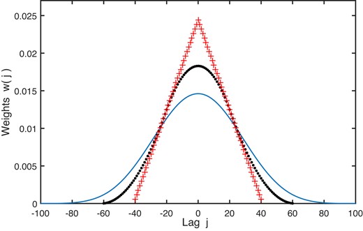
Effective filter weights corresponding to repeated passes of an MA filter with length 2L + 1 = 41. Plus signs: k = 2; dots: k = 3; solid line: k = 5.
Use will also be made of a Fourier transform (FT)-based filter: taking the Fourier transform of Y(t), setting the transform zero for all frequencies higher than a selected limit fC, and then taking the inverse transform. The two filters will, respectively, be referred to as the MAk (k applications of the simple moving average) and the FT filter in what follows.
The choice of the filter bandwidths (filter window length L and number k of applications of the MA filter, or cut-off frequency fC) can be guided by the frequency resolution of the data. The time between successive TESS observations is constant, hence time can conveniently be treated as a discrete variable. With time-steps set to unity, the Nyquist frequency is then 0.5. The frequency resolution is ∼1/N, and setting fC ∼ iC/N with iC = 2–4 ensures that most unwanted frequencies are excluded, but allows variations near ω0 to be captured. As far as the MA filter is concerned, k = 2–4 passes with filter length L = [P] (where [P] = [2π/ω0] is the nearest integer approximation to the period of interest), delivers results similar to those of the FT filter. Examples of frequency transmission functions
can be seen in Fig. 7; note that for this purpose the FT filter was also cast in the typical form (4).
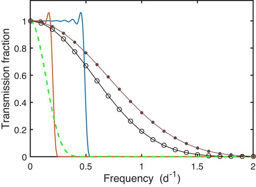
Transmission functions of low-pass filters used in this paper. Solid blue line: FT filter, fC = 0.5 d−1. Solid red line: FT filter, fC = 0.2 d−1. Broken line: MA2 filter, f0 = 1 d−1. Line with open circles: MA3 filter, f0 = 5 d−1. For purposes of comparison, the line with dots shows the transmission of the MA2 filter, f0 = 5 d−1.
Evaluation of CDM results is aided by knowledge about possible bias, and about the random variability of the estimates. The FT filter applied to x(t) is defined by the equations
where the set K of indices in the last equation is chosen to give the desired frequency cut-off fC. Of interest is the real part
of Z, where Xr and Xi are the real and imaginary parts of X. It follows that
A closed form of the function S(t, j) is derived in Appendix A.
From (3), the FT estimates of the amplitude and phase functions are then
where Zrc and Zrs are obtained by, respectively, setting x(j) = y(j)cos (ωj) and x(j) = y(j)sin (ωj) in (6).
Simulation experiments reveal that bias is dominated by the specifics of the filter, and that noise plays a negligible part. Setting y(t) = A cos (ωt + ϕ), i.e. assuming constant amplitude and phase,
In other words, bias is given simply by |$A-\tilde{A}(t)$| and |$\phi -\widetilde{\Phi }(t)$|.
Similarly, applying the MA1 filter to y(t) = Acos (ωt + ϕ),
where D = D(ω, L) is defined in equation (B2). More generally, for an MAk filter,
and hence
To summarize, equations (8) and (9) provide the basis for calculating bias in the estimated amplitude and phase functions. In order to judge the importance of the bias, knowledge of the random estimation errors in these quantities is required. (Bias may be of little importance in the presence of large errors). Uncertainties in the estimated amplitude and phase estimates are induced by the random errors e(t) in (1). In order to study these uncertainties, it is assumed that the smoothing reduces the second term on the RHS of (2) sufficiently compared to the first that it can be ignored. For y(t) of the form (1), with constant amplitude A and phase ϕ, it then follows that
where h(t) = r(t) + is(t) is the smoothed version of the error term e(t)exp (−iωt). For example, for the MA1 filter,
Substituting equation (10) into equation (3), and assuming that the signal to noise ratio (SNR) is sufficiently large that higher order terms in r/A and s/A are negligible,
It follows that
For both types of filter under consideration the functions r(t) and s(t) are linear combinations of the errors e(t). Therefore, the expected values Er = Es = 0, provided Ee = 0 (zero-mean errors). Consequently
Using the results in Appendix C,
for the FT filter. As it happens, the summations in (14) are proportional to N, and independent of ω and ϕ, except for values of t near its extremes. This implies that the variances in (14) are mostly ∝1/N.
For an MAk filter,
In considering numerical examples, we first discuss the simple cases of bias and variance of the estimates from an MAk filter. Note that the factor D in (9) is of order unity; this implies that the bias terms are ∼1/(2L + 1)k. The shortest period in Table 1 is 0.2 d, which covers L = 144 time intervals at 2 min cadence, i.e. the bias terms are of the order 10−5 for k = 2. Even at 30 min cadence with L = 10, bias is of the order 0.002 for k = 2 or 10−4 for three applications of the MA filter. For longer periods, the bias is even smaller.
The standard errors on the estimated amplitudes and phases are characterized by sinusoidal variations with amplitudes which are very small compared to their mean values; it is therefore sufficient to focus on the mean values (over t). The scaling of the errors with A and σe are evident from (15). Scaling aside, errors on |$\tilde{A}(t)$| and |$\tilde{\Phi }(t)$| are closely similar. Furthermore, mean errors are very weakly dependent on N and ϕ, being strong functions of the frequency f only – see Fig. 8. The points in the diagram are well fitted by cubic polynomials
see Table 4 for the coefficients aj. Note that the faster the cadence, the shorter the unit of time, and hence the longer a given period in those time units. This then gives rise to larger smoothing lengths 2L + 1, which again diminishes standard errors.

Standard errors of the estimated amplitudes and phases for the MA2 (squares), MA3 (dots), and MA4 (circles) filters. From top to bottom, cadences are 30, 10, and 2 mins. Also shown is an example cubic fit to the MA2 errors associated with a 30 min cadence. The amplitude A and noise standard deviation σe were set to unity for these calculations.
The results of fitting cubic functions to the mean standard errors on amplitudes and phases estimated by MA filters. The second column specifies the number of applications of the simple MA filter.
| Cadence (min) | k | a3 | a2 | a1 | a0 |
| 2 | 2 | 1.2825E-4 | −2.0598E-3 | 1.7692E-2 | 1.4722E-2 |
| 3 | 1.1650E-4 | −1.8710E-3 | 1.6070E-2 | 1.3372E-2 | |
| 4 | 1.0876E-4 | −1.7468E-3 | 1.5002E-2 | 1.2483E-2 | |
| 10 | 2 | 3.0656E-4 | −4.8401E-3 | 3.9911E-2 | 3.2648E-2 |
| 3 | 2.7844E-4 | −4.3962E-3 | 3.6251E-2 | 2.9654E-2 | |
| 4 | 2.5995E-4 | −4.1042E-3 | 3.3843E-2 | 2.7684E-2 | |
| 30 | 2 | 5.3047E-4 | −8.5718E-3 | 6.8442E-2 | 5.6774E-2 |
| 3 | 4.8182E-4 | −7.7863E-3 | 6.2166E-2 | 5.1567E-2 | |
| 4 | 4.4982E-4 | −7.2690E-3 | 5.8937E-2 | 4.8142E-2 |
The situation for the FT filter is considerably more complicated. In order to put bias into context, it is useful to first consider standard errors (SEs). These exhibit a noticeable dependence on all parameters. Inspection of Fig. 9, for example, shows the influence of the cut-off and signal frequencies. Note, for example, the increase with decreasing fC of the mean levels of all standard errors. The amplitude and phase SE plots are mirror images with respect to the mean error levels, or, put differently, the two curves are 180° out of phase.
Standard errors of estimated amplitudes (solid lines) and phases (dotted lines) for the FT filter for two different cutoff frequencies fC = 0.2 (top panel) and fC = 0.5 (bottom panel). Red and black lines are for signal frequencies 1 and 5 d−1, respectively. Parameters which are the same for all calculations are A = σe = 1, ϕ = 0 and N = 5000 and cadence 2 min.
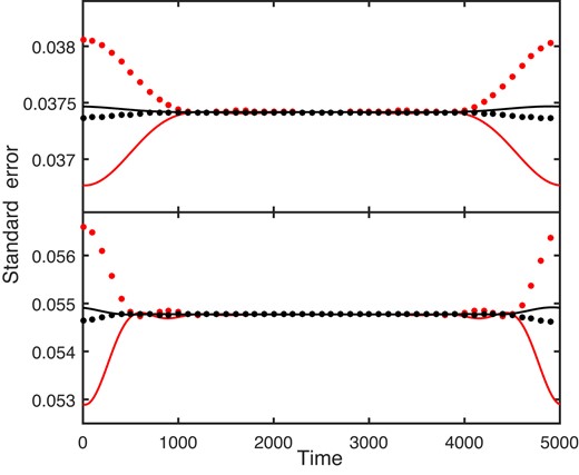
Changing the (constant) phase ϕ changes primarily the first and last ∼10 per cent of the SE series, both in shape and amplitude (Fig. 10). The affected region is smaller for larger sample sizes. Note that although the deviations from the mean levels in Fig. 10 look impressive, the maximum excursions are only 1.6 per cent of the mean.
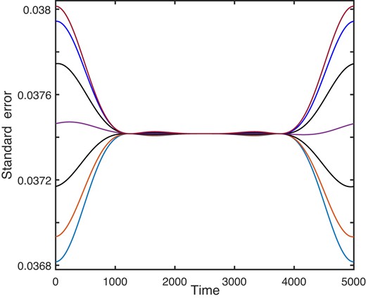
The effect of the phase ϕ on the standard errors in the estimated amplitude. The bottom-most (at time = 1) curve is for ϕ = 0.5; thereafter, successive increments of 0.25 in ϕ lead to steadily increasing errors. Further increases (beyond ϕ = 2) cause the trend to reverse. All calculations assumed a signal frequency f0 = 2.5 d−1, 2 min cadence, fC = 0.2, and A = σe = 1.
The levels of the flat parts of the graphs in Figs 9 and 10 are largely independent of all variables except N: see Table 5, and the illustrative example in Fig. 11. The discontinuity in the latter graph is due to a change in the number of low frequencies taken into account (i.e. ic changes from 2 to 3 at N ≈ 7200).
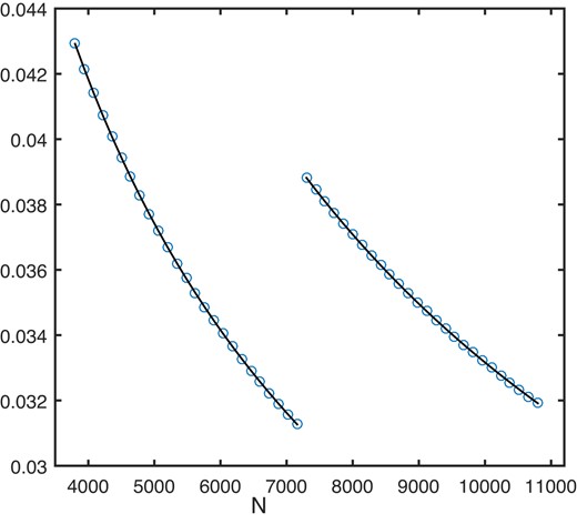
Standard errors on the FT estimated amplitude or phase for 2 min cadence data with cut-off frequency fC = 0.2 d−1 (small circles). The scaling is such that A = σe = 1. The fitted lines are of the form |${\rm SE}=\beta/\sqrt{N}$|, where β = 2.6458 (N ≤ 7200), 3.3166 (N > 7200).
The results of fitting the relation SE|$=\beta /\sqrt{N}$| to the mean standard errors on amplitudes and phases estimated by FT filters.
| Cadence (min) | Range N | β | Range N | β |
| Cutoff frequency 0.2 d−1 | ||||
| 2 | 3601–7200 | 2.6458 | 7201–10800 | 3.3166 |
| 10 | 1441–2160 | 3.3166 | – | – |
| 30 | 241–480 | 2.6458 | 481–720 | 3.3166 |
| Cutoff frequency 0.5 d−1 | ||||
| 2 | 4321–5760 | 3.8730 | 5761–7200 | 4.3589 |
| 7201–8640 | 4.7958 | 8641–10080 | 5.1962 | |
| 10 | 1441–1728 | 4.7958 | 1729–2016 | 5.1962 |
| 30 | 385–480 | 4.3589 | 481–576 | 4.7958 |
| 577–672 | 5.1962 | – | – | |
Armed with this information about standard errors, we are able to sensibly evaluate the bias in |$\widetilde{A}(t)$| and |$\widetilde{\Phi }(t)$| estimated by the FT filtering. Fig. 12 is the bias-related counterpart of Fig. 9: there is a qualitative similarity between the diagrams in the sense that constant variance or low bias is generally restricted to the inner part of the time interval. As for the SEs, the precise form of the bias is sensitive to the phase ϕ. Comparing the two figures shows that the bias is within 1 SE for the configuration shown, i.e. not of major concern.
Expected values of the amplitude (top panel) and phase (bottom panel) functions, for 2 min cadence data with cut-off frequency fC = 0.2 (thin lines) or 0.5 d−1 (thick lines). Red (black) lines correspond to a signal frequency of 1 d−1 (5 d−1). The assumed (constant) amplitude and phase are A = 1 and ϕ = 0.
In general, the importance of the bias should be considered against the background of the scaling with σe and A in equations (8) and (14). For example, if A = 10, the amplitude bias in Fig. 12 is increased tenfold, while its SE is unaffected. Although the phase bias is unaffected, its SE is decreased tenfold, and hence its bias may be highly significant.
Since the bias is a cause of concern only near the beginning and end of the time series, the simplest way of dealing with it is to discard estimates over the two intervals [1, ℓ] and [N − ℓ, N]. One option is to choose ℓ such that the bias over the interval [ℓ + 1, N − ℓ − 1] is at most one sigma. This often proved overly restrictive, leading to unacceptably large ℓ. Replacing σ by 10 per cent of the range of |$\widetilde{A}$| or |$\widetilde{\Phi }$|, where the estimates are computed by an MA filter, seemed like a reasonable compromise. This follows because the resulting ℓ is smaller, but any bias is also guaranteed to be small in relative terms. Furthermore, a minimum of 2.5 per cent of N was trimmed off either end of the series of FT estimated amplitude and phase functions, to avoid obvious end effects (as visible in e.g. Fig. 12).
4 RESULTS
All the demodulation results are available as supplementary material to the paper; Figs 13 and 14 are examples. Fig. 13 is derived from the sector 29 photometry of CD66 (see Fig. 4, and the top panel of Fig. 15), and Fig. 14 from the sector 6 photometry of CD36 (see the bottom two panels of Fig. 15).
Estimated amplitude and phase variations of the periodicity in the sector 29 photometry of CD66 (first orbit results on the left). Note the abrupt decrease in the amplitude during the first orbit, accompanied by a switch in the direction of the phase change. Black and red lines are estimates from the FT and MA filters, respectively. The short vertical bars in the bottom left corner of each panel are two SEs in length.
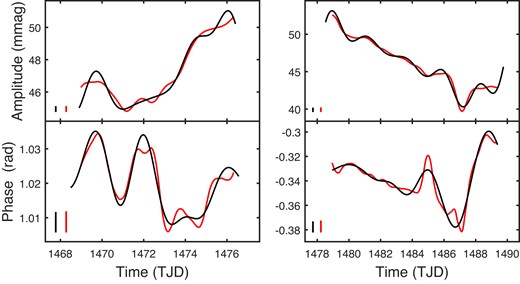
Estimated amplitude and phase variations of the periodicity in the sector 6 photometry of CD36 (first orbit results on the left). The rapid, small amplitude change and recovery near TJD 1487 are clearly visible in the light curve (Fig. 15). Black and red lines are estimates from the FT and MA filters, respectively. The two short vertical bars in the bottom left corner of each panel are two SEs in length.
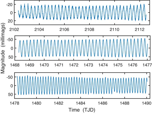
The top panel shows the second orbit, sector 29, in the photometry of CD66. (The first orbit observations are plotted in Fig. 4). The middle and bottom panels contain plots of the sector 6 light curves of CD36. In the bottom panel, note the elevated level of light minimum following a (removed) flare at TJD 1486.8.
Note that fC = 0.5 and k = 3 for all the data sets except the CD-49 1902 observations; for those fC = 0.2 (because of its longer period of 1.108 d) and k = 2. The latter choice was dictated by the relatively short data strings for this star, and the desire to avoid ‘losing’ too many observations through repeated applications of the MA filter. In general, the agreement between the FT and MA filter results is good.
In each of the plots, pointwise uncertainties (from equations 14 and 15) are indicated by vertical bars of length 2 SE. In order to gauge whether the overall estimated variability is meaningful the ranges of |$\widetilde{A}(t)$| and |$\widetilde{\Phi }(t)$| were calculated, and standardized by σA and |$\sigma _\Phi$|, respectively. The standardized ranges were generally well above 10, with only eight estimated functions having ranges below 8. To put this into context, Fig. 16 shows simulated 99-th percentiles of the estimated range, for a number of data set sizes and assumed frequencies f0. The simulations were carried out only for the simpler case of the MA filter (i.e. with minimal bias). As can be seen in the figure, the percentiles are sensitive functions of the series length N and the signal frequency f0; there is little or no dependence on the values of A, σe, and ϕ.
![The 99-th percentiles of simulated distributions of the standardized amplitude range (i.e. range$[\widehat{A}(t)]/\sigma _{\rm A}$), when the amplitude and phase are constant. Circles, diamonds, and squares are for f0 = 1, 2.5, and 5 d−1, respectively. Results are for the MA2 filter (f0 = 1) and MA3 filter (the two higher frequencies), assuming a 2 min cadence. Overlapping symbols correspond to different assumed A and ϕ. Percentiles for the standardized range of $\widehat{\phi }$ are very similar.](https://oup.silverchair-cdn.com/oup/backfile/Content_public/Journal/mnras/528/2/10.1093_mnras_stae161/1/m_stae161fig16.jpeg?Expires=1749329612&Signature=FhTpryKXPOIKlp4wTOv5zuJNpuKJUchLl~2a~yZhhHPYNIsSslyW2a4Yz3FfuvvHLtjn~fc544Xm1qyGlY9Y6IwZwf9M5OMkdXIvOGDEWP8GH0iXGSFHFIspQPSGAHhmn6n7bPx5NffAbdoA6HCWk5oZZO8IHTxsd1JvRwi4W2gH2wA1sFg~aw3woQEAOh3u2fVhdxeJ6qyEXCejrJuleH71oa6~5n0GsizZ32j4DZgGZXnJItUuWYQ02EDUhu9JTvVEfXYhTYMGise9fJupKXMDtX34TCIHzKAY01F0DcfxRGEvQMQgUYZ8iJxJFuYalz0cEX2O4DIPnxwAckMoWg__&Key-Pair-Id=APKAIE5G5CRDK6RD3PGA)
The 99-th percentiles of simulated distributions of the standardized amplitude range (i.e. range|$[\widehat{A}(t)]/\sigma _{\rm A}$|), when the amplitude and phase are constant. Circles, diamonds, and squares are for f0 = 1, 2.5, and 5 d−1, respectively. Results are for the MA2 filter (f0 = 1) and MA3 filter (the two higher frequencies), assuming a 2 min cadence. Overlapping symbols correspond to different assumed A and ϕ. Percentiles for the standardized range of |$\widehat{\phi }$| are very similar.
The conclusion is that estimated variability is significant at at least the 0.5 per cent level for all but three estimated functions – |$\widehat{\Phi }$| for CD49 (sector 6a) and CD56 (f0 = 2.39 d−1, sector 12b) and |$\widehat{A}$| for CD49 (sector 5a). There is a caveat to this, though: the standard errors σA and |$\sigma _\Phi$| were calculated from (13), which is based on the assumption that the SNR is large. It is easy to see that should the amplitude approach zero, the phase will become indeterminate, and hence |$\sigma _\Phi$| will increase without bound. In reality, SNRs below 5 are seen at some times for all data sets (except for CD72, f0 = 4.245 d−1), as can be seen from the amplitude spectra in the supplementary material.
CDM reveals a variety of shapes of amplitude and phase changes over the course of single orbits, i.e. over time-scales of a few days. Forms include: roughly linear (CD49 sector 7b; CD66 sectors 13b, 28, 30), linear with ripples (CD66 sectors 27b, 39a; CD72 sectors 1a, 7a, 9a, 34b), roughly quadratic (CD49 sector 5b; CD56 sector 37b; CD66 sector 38b; CD72 sector 28b), abrupt level shifts (CD36 sector 34b; CD66, sectors 9b, 10a; CD72, sector 27b), oscillatory (CD56 sectors 11b, 27a, 28a; CD66 sector 35a; CD72 sectors 8a, 11a, 12b, 37a, 37b), broad pulses or troughs (CD56 sectors 8a, 8b, 10b, 12a, 31b; CD66 sectors 35b, 37b; CD72 sectors 1b, 4a, 28b), narrow pulses or valleys (CD36 sectors 6b, 7b; CD56 sectors 5b, 7a; CD72 sector 4a), and quite complex variability (CD66 sector 32b; CD56 e.g. sectors 34a, b; CD72 e.g. sectors 11b-27b). In general, there does not seem to be any relationship between amplitude and phase changes, nor (in the cases of CD56 and CD72) changes in attributes of the two unrelated frequencies.
We discuss a few specific cases in more detail. The abrupt amplitude change visible in the sector 29a light curve of CD66 (Fig. 4) is reflected in its |$\widehat{A}(t)$| plot (Fig. 13). What is not obvious from the light curve is that in this case there is an accompanying change in the phase. Examination of |$\widehat{\Phi }$| shows that it can be interpreted as two roughly linear sections, with a switch between the two during the short time (∼1 d) during which the amplitude decreases rapidly. Instead of two gradual phase changes, this could be interpreted as a switch between two frequencies. A possible physical basis is a rapid change in the latitude at which star-spots dominate, together with differential rotation of the stellar surface.
Fig. 14 presents a somewhat different scenario: the dip in |$\widehat{A}$| during the sector 6b observations of CD36 can be traced to the obvious temporary elevation of the light curve minimum (Fig. 15). This again appears to be the result of a short-lived flare at TJD 1486.85. The flare, which happened near the phase of minimum, appears to affect the level of the minimum only for a few cycles. An explanation is that the flare left a bright region on/near the star at its darkest site; the bright region then gradually faded from view.
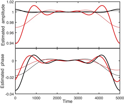
Whereas amplitude changes are often obvious in the light curves, phase changes are generally quite small, typically smaller than 2 per cent of a cycle. Though the estimated ranges of variation are almost without exception highly significant, the reader may wonder how accurately the functions |$\widetilde{\Phi }(t)$| are. Fig. 17 shows the results of applying CDM to two simulated time series with different signal frequencies. The phase was taken to vary as
while the amplitude was kept constant. Realistic amplitudes, noise levels, and series lengths were assumed. For the higher frequency (f0 = 5 d−1) in the top panel, estimates from both filters are evidently highly accurate. The FT filter also performs well for the lower frequency (f0 = 2 d−1, bottom panel), while the MA3 filter oversmooths, leading to an underestimation of the amplitude of the variations. Fortunately, only two of the seven signal frequencies in the paper are of the order of 2 d−1 or lower, so that this should not be a substantial problem. Note also that a smaller MA filter order (k = 2), and hence less smoothing, was used for the real CD49 data for which f0 = 1.1 d−1.
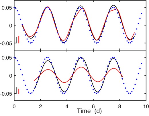
Estimated phase functions |$\widetilde{\Phi }(t)$| for signals with a constant amplitude A = 15 and noise standard deviation σe = 2.3. Black and red lines, respectively, denote estimates from the FT filter (fC = 0.5) and MA filter (k = 3), while dots show the true values. Short vertical bars denote 2|$\sigma _\Phi$|. The cadence (2 min) and number of data (N = 7000) are typical of most data sets. Top panel: f0 = 5 d−1. Bottom panel: f0 = 2 d−1.
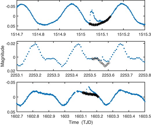
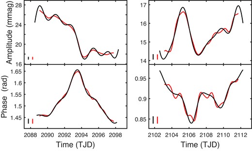
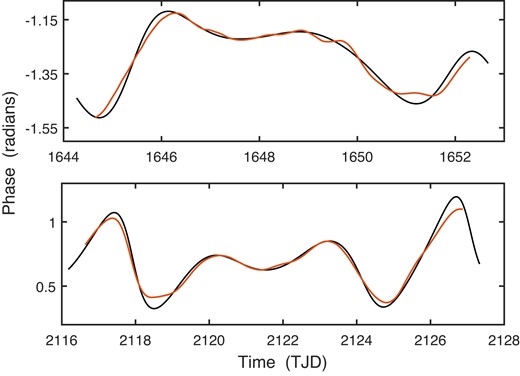
Two examples where phase changes in light curves are visually discernible are given in Fig. 18. Note that in both data sets harmonics of the frequency of interest, as well as the second frequency and its harmonics, have been pre-whitened from the photometry, leaving only one sinusoid. In the top panel (CD56, sector 12b), observations lead the model light curve at the outset, but by TJD 1645.5 the situation reverses. At the end of the light curve section, the two curves are approximately in phase. Similarly, in the bottom two panels (CD72, sector 30a), observations lead at the start, but lag by TJD 2124.7. For most of time depicted in the bottom panel, observations again lead the model light curve.
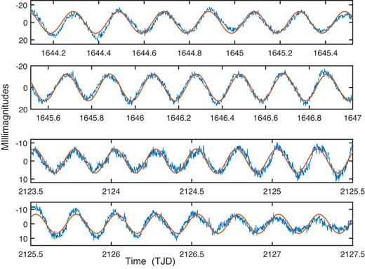
Blue lines: sector 12b variability of CD56 at f = 5.01 d−1 (top two panels) and sector 30a variability of CD72 at f = 3.98 d−1 (bottom two panels). Red lines: fitted model light curves, assuming constant amplitude and phase. See the text for more details.
The estimated phases of the two frequencies over the entire orbits are plotted in Fig. 19. The large roughly linear drifts in phase over 1644.6 < TJD < 1646.3 (top panel) and 2124.7 < TJD < 2126.8 (bottom panel) can alternatively be interpreted as manifestations of frequency jumps. This follows because the instantaneous frequency of a sinusoidal signal
is defined as
Consequently, if
where α is the slope of the phase drift, then the instantaneous frequency is f(t) = f0 + α/2π, a change of α/2π d−1 from the frequency f0 at at t = t0. The implied frequency shifts are ∼0.04 (CD56) and ∼0.06 d−1 (CD72), i.e. fractional changes of 0.8 and 1.6 per cent, respectively.
Estimated phase changes in the f = 5.01 d−1 frequency of C56 during sector 12b (top panel), and in the f = 3.98 d−1 frequency of CD72 during sector 30a (bottom panel).
The combined CDM results for all the sectors are plotted in Fig. 20, for CD66 (see Supplementary material for the other stars). Since the phase zero-points for each orbit is essentially arbitrary, the mean phase value for each orbit has been set to zero.
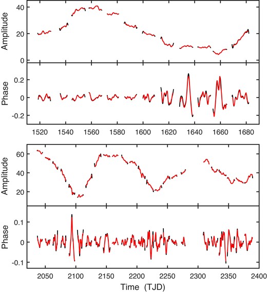
All estimated amplitude and phase changes in the periodic variations of CD66. Top two panels: sectors 8–13. Bottom two panels: sectors 27–39 (excluding 36). Amplitudes are in millimagnitudes, phases in radians. Black and red lines, respectively, show FT and MA filter results.
A noteworthy feature of the diagrams is that the phase variability appears to be greatly enhanced when the amplitude is low – see, for example, near TJD 1660 and 2100 in Fig. 20, or at the beginning and end of the first season of the CD72 data (for f2 = 3.9785 d−1). The phase standard errors are, however, larger at smaller amplitudes [equations (14) and (15)], so that this is a point which should be studied in greater depth.
The estimated functions |$\widetilde{A}(t)$| and |$\widetilde{\Phi }$| over all orbits were scrutinized for periodicities, but none were found. This is perhaps one of the most important findings of this paper: although Fig. 20 (and other such plots in the Supplementary material) suggest cycles in the photometric amplitudes, the changes are aperiodic.
The estimated functions are freely available for further analysis.
5 MORE ON THE BINARITY OF CD56 AND CD72
As seen above, photometry of two of the stars, CD56 and CD72, show the presence of two independent periods. (All stars show multiple periodicities, but in the other three cases these consist of fundamental frequencies plus harmonics). A reasonable explanation is that these two stars are binary WTTSs.
One possible means of investigating binarity is to try model the observed spectral energy distribution (SED) by the sum of two theoretical SEDs. This would clearly only be useful if the SEDsof the two star were rather different. However, if one star were substantially cooler than the other, it would also need to be larger in order for its radiation to be detectable at all: this seems unlikely for two coeval young stars. The situation would be further complicated by non-photospheric radiation excesses in the blue and/or red – as observed for the present set of stars.
Although only a few radial velocity measurements are available, it does appear that CD72 may be a radial velocity variable (Table 1). Furthermore, according to Table 2, CD56 and CD72 are the most luminous of the five stars, albeit not by much. None the less, bearing in mind that the contribution by a hidden binary companion is at most −0.75 mag, the small luminosity excesses in CD-56 1438 and CD-72 248 may none the less be meaningful.
Gaia radial velocity data (Katz et al. 2023) for the stars were also extracted from the Gaia archive.6 The ‘rv_chisq_pvalue’, which assesses the probability that the radial velocity is constant, is zero for all five stars. Similarly, the constant-velocity goodness-of-fit (GOF) statistics lie in the range 14.9–48.4; given that this measure has a standard normal distribution, these values are all highly indicate of variability.
In order to put these results into context, data for 66 WTTSs from the lists of Padgett et al. (2006) and Gregorio-Hetem & Hetem (2022) were also retrieved from the Gaia archive. Of these, 55 satisfy the criteria n ≥ 10 (minimum number of transits) and 3900 ≤ Teff ≤ 8000 K (Katz et al. 2023). The χ2p-values of only six stars are not significant at the conventional 5 per cent level; 47 have p < 0.001. It therefore seems that measured radial velocity variability is a very common feature of WTTSs, being present for 85 per cent of the sample. It is not clear whether this could simply be a result of spectral variability, or whether it truly points to stellar multiplicity.
Kounkel et al. (2022, 2023) (and references to earlier work therein) have made the point that rapidly rotating PMS stars are predominantly in binary systems. It would therefore be interesting to conduct a larger study than the modest one reported above and to correlate radial velocity variability measured by Gaia with rotation periods.
The third Gaia data release contains information for ‘non-single stars’ (NSS – Gaia Collaboration 2023a,b). Interestingly, of the five stars studied in this paper, only CD56 is a Gaia NSS, namely an astrometric multiple. The binary solution has (T1 ≈ 4975 K, log g1 ≈ 4.23); (T2 ≈ 5150 K, log g2 ≈ 4.78). It is noteworthy that the second temperature in Table 2 lies between these two values.
As a point of interest, three of the 66 randomly selected WTTSs are Gaia NSS: RX J1524.0-3209, RX J1525.5-3613 and Wa Oph 1.
6 CONCLUDING REMARKS
There is a large literature on the topic of long-term cycles in magnetic-related activity in stars, i.e. analogues of the solar cycle – see e.g. Distefano et al. (2017), Mignon et al. (2023), Irving et al. (2023), and numerous references therein. Conclusions from different studies of the same stars are often contradictory (see e.g. Mignon et al. 2023). The methodology is sometimes questionable – for example, identifying periodicities by eye when formal methods reveal none. Furthermore, the author is not aware of a single instance in which three or more cycles of the same putatively long periodicity in stellar activity have been seen (except in the obvious case).
The confusion is easily explained by the type of long-term variability amplitudes found in the present five cases, namely random, aperiodic changes. It is not difficult to identify apparent periodicities in sections of such series, particularly if they are only observed intermittently. It is also important to note that the type of amplitude variability seen in Fig. 20 is not necessarily even ‘quasi-periodic’. True non-regular periodicities are described by second-order differential equations (as in the case of their deterministic counterparts), but first-order stochastic differential equations can also exhibit what appear to be cycles (see e.g. the discussion in Wright et al. 2006), although these are completely transient.
A number of aspects of the methodology described above deserve further exploration. Amongst these, perhaps the most obvious is to find objective methods to determine the ‘best’ values of the cut-off frequency fC of the FT filter and the number of applications k of the MA filter. Another issue is the development of a formal test procedure in order to establish whether there is indeed an inverse correlation between the level of phase variability and the amplitude A(t).
One possible way to obtain better error estimates is to use bootstrapping (e.g. Efron & Tibshirani 1993). In the present context, this would entail the following:
- Calculate the estimation residualswhere m(t) is the estimated model, and L1 and L2 are the lower and upper limits of the times for which estimates |$\widetilde{A}$| and |$\widetilde{\Phi }$| are available.(16)$$\begin{eqnarray} \widehat{e}(t)&=&y(t)-m(t) \\ m(t)&=&\widetilde{A}(t) \cos [\omega _0 t + \widetilde{\Phi }(t)],{\qquad}L_1 \le t \le L_2, \end{eqnarray}$$
Draw, with replacement, a random sample of size L2 − L1 + 1 from the set of |$\widehat{e}$|. Add these to the model values m(t) to produce a set of pseudo-observations y(1)(L1), y(1)(L1 + 1), …, y(1)(L2).
Apply the CDM methodology to the y(1)(t), producing estimates |$\widetilde{A}^{(1)}(t)$| and |$\widetilde{\Phi }^{(1)}(t)$|. Note that another n1 and n2 datapoints will be lost, respectively, at the start and end of the interval [L1, L2], due to low pass filtering.
Repeat steps (ii) and (iii) M − 1 times, generating data sets {y(j)(t)} followed by estimated functions |$\widetilde{A}^{(j)}(t)$| and |$\widetilde{\Phi }^{(j)}(t)$|.
For each time point, L1 + n1 + 1 ≤ t ≤ L2 − n2 percentiles for the original |$\widetilde{A}(t)$| and |$\widetilde{\Phi }(t)$| can now be constructed from the M bootstrapped amplitude and phase function values at the specific time point.
Of course, such a procedure would be computationally intensive. It also has the drawback that, due to the smoothing losses, it is only useful over the central part of the observation interval.
It has been implicitly assumed in equation (1) that the errors e(t) are uncorrelated. Should this not be the case, then equations such as (14) and (15) need to be amended: the measurement error is no longer a constant, but instead depends on frequency. As shown by Hannan (1971) and Walker (1973), |$\sigma _{\rm e}^2$| is replaced by I(f0), where I is the power spectrum
and γ(k) is the autocovariance function of the noise process e(t), at lag k.
ACKNOWLEDGEMENTS
This research has made use of the VizieR catalogue access tool and the Simbad Astronomical Database at CDS, Strasbourg, France; bolometric corrections from the ‘MESA Isochrones and Stellar Tracks’; and the results of various large photometric surveys referred to in section 1 of the paper. The paper is based on data collected with the TESS mission, downloaded from the MAST data archive at the Space Telescope Science Institute (STScI). The paper benefitted from the referee’s comments.
DATA AVAILABILITY
TESS photometry is available from the website given in section 2. The data underlying the supplementary figures are available from the author.
Footnotes
References
APPENDIX A: A SUMMATION FORMULA FOR THE FT FILTER
The required sum is
The set K of indices is related to the low pass filter cut-off frequency fC:
where the square brackets indicate the integer part of the number. Note that 0 < fC ≤ 0.5, i.e. time is defined in units of the cadence, so that the Nyquist frequency is 0.5. The set of indices is then
Consequently
Using the formula
(e.g. Gradshteyn & Ryzhik 2007) we obtain
and
APPENDIX B: A SUMMATION FORMULA FOR THE MA FILTER
Let
In order to make use of the summation formula
(e.g. Gradshteyn & Ryzhik 2007), (B1) is rewritten as
where the shorthands ω′ = 2ω and ϕt = ϕ + 2ωt were used. Similarly, the identity
can be used to show that
It follows that for k repeated applications of the filter
APPENDIX C: EXPECTATIONS OF SMOOTHED NOISE FUNCTIONS
The functions r(t) and s(t) are smoothed versions of e(t)cos (ωt) and e(t)sin (ωt) [see the discussion between equations (10) and (11)]. As such, for the FT filter, use can be made of equation (5), with x(j) replaced by the appropriate function:
where S(t, j) is defined in equations (A1) and (A2). If e(t) is a zero-mean white noise series,
hence
For the MA1 filter,
More generally, for an MAk filter,
with w(j) a weight function such as in Fig. 6.
