


ABSTRACT
The recent decade has seen an exponential growth in spatially resolved metallicity measurements in the interstellar medium (ISM) of galaxies. To first order, these measurements are characterized by the slope of the radial metallicity profile, known as the metallicity gradient. In this work, we model the relative role of star formation feedback, gas transport, cosmic gas accretion, and galactic winds in driving radial metallicity profiles and setting the mass–metallicity gradient relation (MZGR). We include a comprehensive treatment of these processes by including them as sources that supply mass, metals, and energy to marginally unstable galactic discs in pressure and energy balance. We show that both feedback and accretion that can drive turbulence and enhance metal-mixing via diffusion are crucial to reproduce the observed MZGR in local galaxies. Metal transport also contributes to setting metallicity profiles, but it is sensitive to the strength of radial gas flows in galaxies. While the mass loading of galactic winds is important to reproduce the mass–metallicity relation (MZR), we find that metal mass loading is more important to reproducing the MZGR. Specifically, our model predicts preferential metal enrichment of galactic winds in low-mass galaxies. This conclusion is robust against our adopted scaling of the wind mass-loading factor, uncertainties in measured wind metallicities, and systematics due to metallicity calibrations. Overall, we find that at z ∼ 0, galactic winds and metal transport are more important in setting metallicity gradients in low-mass galaxies whereas star formation feedback and gas accretion dominate setting metallicity gradients in massive galaxies.
1 INTRODUCTION
Metals act as natural tracers of galaxy evolution and provide some of the most important constraints on the physical properties of baryons in galaxies (Kobayashi, Karakas & Lugaro 2020). This has resulted in the development of several galactic chemical evolution models over the last three decades to reproduce, fit, or explain trends in the metal content of galaxies. Most of the literature thus far has focused on understanding the physics of galaxy-integrated (or global) metallicities, and fundamental trends such as the mass–metallicity relation (MZR; Tremonti et al. 2004; Zahid et al. 2014; Sanders et al. 2021). However, thanks to integral field unit (IFU) spectroscopy, the last decade has seen immense advancements in mapping the spatially resolved metal content in galaxies. It is now clear that, at least at z = 0, galaxies typically exhibit a gradient in metallicity whereby their inner parts are more metal rich than their outskirts. Such a negative metallicity gradient is a natural consequence of inside–out galaxy formation (e.g. Shaver et al. 1983).
This simplified picture is complicated by various factors internal and external to galaxies, as is evident from the vast diversity of metallicity gradients discovered in numerous galaxies across cosmic time (see reviews by Kewley, Nicholls & Sutherland 2019; Maiolino & Mannucci 2019; Sánchez 2020). High-resolution data from IFU spectroscopy have also revealed the existence of resolved versions of the MZR: the mass–metallicity gradient relation (MZGR) and the resolved mass–metallicity relation (rMZR). The former describes the evolution of metallicity gradients with stellar mass (e.g. Sánchez et al. 2014; Belfiore et al. 2017; Sánchez-Menguiano et al. 2018; Poetrodjojo et al. 2018; Mingozzi et al. 2020; Sharda et al. 2021b; Franchetto et al. 2021), whereas the latter describes the evolution of local metallicity with the local stellar surface density (e.g. Rosales-Ortega et al. 2012; Sánchez et al. 2013; Barrera-Ballesteros et al. 2016; Trayford & Schaye 2019).
IFU observations have started to reveal the detailed 2D structure of metal distribution in galaxies, finding evidence not just for radial, but also azimuthal variations (e.g. Ho et al. 2017, 2018; Kreckel et al. 2019, 2020; Li et al. 2021, 2023). However, progress in theoretical work on modelling these first- and second-order metallicity variations for a wide range of galaxies has remained rather limited (Kudritzki et al. 2015; Ho et al. 2015; Lian et al. 2018; Krumholz & Ting 2018; Belfiore et al. 2019; Sharda et al. 2021a; Metha, Trenti & Chu 2021). A key challenge in modelling resolved metal distributions is that they are impacted by both local and global processes in galaxies (Baker et al. 2023; see, however, Boardman et al. 2022). Additionally, while the global metallicity is only sensitive to the total metal content of galaxies, the spatially resolved metallicity structure is also affected by transport processes within the interstellar medium (ISM), which redistribute metals from the time they are produced. Thus, metal dynamics are as important as metal production and ejection in setting spatially resolved metal distributions. We subdivide and introduce these two categories below (see also Fig. 1).
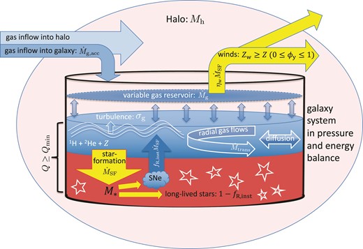
Bathtub model of chemical evolution, adapted from Lilly et al. (2013, fig. 2), and modified to reflect the spatially resolved metallicity model presented in this work. The galaxy is modelled as a two-component reservoir: stellar (red) and gas phase (blue). The gas reservoir is made up of H, He, and metals (denoted by the ISM metallicity Z). We consider marginally unstable galactic discs (quantified by the Toomre Q parameter) in pressure and energy balance. The evolution of gas mass, |$\dot{M}_{\rm {g}}$|, is described by equation (7). It depends on the gas accretion rate (|$\dot{M}_{\rm {g,acc}}$|), star formation rate (|$\dot{M}_{\rm {SF}}$|), radial gas flows (or, gas transport, |$\dot{M}_{\rm {trans}}$|), and galactic winds (|$\eta _{\rm {w}}\dot{M}_{\rm {SF}}$|, where ηw is the mass-loading factor). Gas turbulence (quantified by the gas velocity dispersion, σg) is driven by energy injected into the ISM via accretion, star formation feedback, and gas transport. Metals are produced as star formation leads to supernovae (SNe). Some fraction of the metals produced is returned almost instantaneously to the ISM (fR,inst), whereas the rest is locked in long-lived stars. Metals are also ejected via galactic winds with metallicity Zw, which can be greater than or equal to Z. ϕy denotes the preferential metal enrichment of winds. Once produced, metals are also advected with radial gas flows, and diffused into the ISM due to turbulence and thermal instabilities. ©AAS. Reproduced with permission.
1.1 Gas and metal flows in/out of galaxies
To understand the physics of spatially resolved metal distribution and metallicity gradients, it is helpful to first explore the life cycle of baryons in galaxies. Gas regulator models paint a simple yet powerful picture of this life cycle: gas accretes on to the galaxy from the cosmic web in the form of cold or hot streams, or through mergers and interactions (e.g. Fardal et al. 2001; Dekel & Birnboim 2006; Bournaud & Elmegreen 2009; Dekel et al. 2009a; Rupke, Kewley & Barnes 2010). The accreted gas is then transported across the galactic disc via angular momentum exchange due to viscous torques or encounters with giant molecular clouds (GMCs) and bars or spiral arms (e.g. Pfenniger & Norman 1990; Block et al. 2002; Bournaud, Combes & Semelin 2005; Dekel, Sari & Ceverino 2009b; Krumholz & Burkert 2010; Hopkins & Quataert 2011). The accreted gas also acts as a fuel for star formation, and dictates subsequent galactic life cycles (e.g. Kereš et al. 2005; Somerville & Davé 2015). Star formation leads to metal production dictated by the mass distribution of massive stars following a stellar initial mass function. Some of these metals are locked in low mass stars that live for a long time, others are returned to the ISM on relatively shorter time-scales (Tinsley 1980), or are depleted on to dust (e.g. Konstantopoulou et al. 2022). Star formation and active galactic nuclei (AGNs) feedback drives winds that eject mass and metals out of the galaxy (e.g. Veilleux, Cecil & Bland-Hawthorn 2005; Muratov et al. 2015; Pillepich et al. 2018a; Mitchell et al. 2020a; Veilleux et al. 2020; Pandya et al. 2021). A fraction of the ejected mass makes its way back on to the disc in the form of fountains (e.g. Shapiro & Field 1976; Fraternali & Binney 2008; Grand et al. 2019; Li & Tonnesen 2020), whereas the rest enriches the circumgalactic medium (CGM) with metals (Tumlinson, Peeples & Werk 2017). Sufficiently strong winds can also deposit metals beyond the virial radii of galaxies into the intergalactic medium (IGM; Origlia et al. 2004; Ranalli et al. 2008; Tumlinson et al. 2011). Thus, the life cycle of metals is quite dynamic, and it is now known that all these different physical processes alter the metal content of galaxies (e.g. Dalcanton 2007; Finlator & Davé 2008; Lilly et al. 2013; Grand et al. 2019; Sharda et al. 2021a; Wang & Lilly 2022b; Greener et al. 2022).
1.2 Metal dynamics within galaxies
We define metal dynamics as processes that alter the spatial distribution of metals within galaxies without altering the total metal mass. Broadly speaking, we can further classify metal dynamics into categories: (1) transport of metals with the bulk flow of the gas, and (2) redistribution of metals. The former results in advection of metals, and is primarily driven by radial gas flows generated due to gravitational instabilities (Dekel, Sari & Ceverino 2009b; Krumholz & Burkert 2010; Forbes, Krumholz & Burkert 2012), magnetic stresses (Wang & Lilly 2022a), stellar bars (Kubryk, Prantzos & Athanassoula 2013, 2015), or mismatch in the specific angular momentum of accreting gas and the disc (Mayor & Vigroux 1981; Pezzulli & Fraternali 2016). The latter is caused by turbulence in galactic discs that mix metals produced in different parts of the galaxy (e.g. due to diffusion or thermal instabilities, Yang & Krumholz 2012; Petit et al. 2015; Beniamini & Hotokezaka 2020). Except for a handful of galactic chemical evolution models, most models to date still lack a treatment for metal advection. The few that do include this process find it to be important for setting resolved metallicity trends in galaxies (Sharda et al. 2021a; Chen et al. 2023b). However, the treatment of radial gas flows is often decoupled from star formation and gas accretion, which creates inconsistency in the treatment of metals and the gas, or allows for tunable parameters that are then matched to an observable to constrain metal advection. This is further complicated by the fact that direct evidence for radial gas flows is scarce (Schmidt et al. 2016; Di Teodoro & Peek 2021; Sharda et al. in preparation), even though it has been long suspected to play an important role in galaxy evolution (Tinsley 1980; Lacey & Fall 1985).
The diffusion of metals due to turbulence warrants a detailed discussion since it is a relatively new component of galactic chemical evolution models (Sharda et al. 2021a), and is usually implemented as sub-grid physics in hydrodynamical simulations (Escala et al. 2018). Galactic discs typically exhibit supersonic turbulence, as is now known from measurements of the multiphase gas velocity dispersion across cosmic time (Ianjamasimanana et al. 2012; Moiseev, Tikhonov & Klypin 2015; Wisnioski et al. 2015; Varidel et al. 2016, 2020; Simons et al. 2017, 2019; Wisnioski et al. 2019; Förster Schreiber et al. 2018; Übler et al. 2019; Girard et al. 2021). Simulations have shown that, in the absence of strong anisotropies (Hansen, McKee & Klein 2011; Beattie & Federrath 2020) or strong magnetic fields oriented perpendicular to the disc (Kim & Basu 2013), supersonic turbulence decays very rapidly compared to the dynamical time of the disc (Mac Low et al. 1998; Stone, Ostriker & Gammie 1998; Lemaster & Stone 2009; Downes & O’Sullivan 2009, 2011; Burkhart et al. 2015; Kim & Ostriker 2015b). Therefore, turbulence needs to be continuously driven in galactic discs in order to explain the observed high gas velocity dispersions that cannot be a result of thermal gas motions (Sarrato-Alós, Brook & Di Cintio 2023).
The two most common sources of turbulent energy injection into the ISM in galactic discs are star formation feedback due to supernovae (Ostriker & Shetty 2011; Faucher-Giguère, Quataert & Hopkins 2013) and radial gas flows. Krumholz et al. (2018, hereafter, KBFC18) present a unified model of galaxies that includes both these processes, and show that star formation feedback alone can maintain a floor velocity dispersion of |$6-10\, \rm {km\, s^{-1}}$|, explaining why the gas velocity dispersion tends to settle down to this value. KBFC18 also find that the high gas velocity dispersions seen in starburst galaxies are primarily driven by gravity due to radial mass transport. This model has been used to reproduce the observed star formation rate (SFR) – gas velocity dispersion trend in several surveys (Johnson et al. 2018; Yu et al. 2019; Varidel et al. 2020; Yu et al. 2021; Girard et al. 2021; see also Ejdetjärn et al. 2022). A number of other authors have also published models to explain the role of turbulence in galaxy evolution but without the dual role of feedback and transport while simultaneously considering energy and momentum balance (KBFC18, section 1.2 and references therein).
However, KBFC18 only consider gas accretion from outside the galaxy as a source that supplies mass to the galactic disc, but did not consider the possibility that it might also drive turbulence in the disc (Ginzburg et al. 2022). Such driving is possible because the accreting gas can convert some of its kinetic energy into turbulence, as has been demonstrated in several simulations (Klessen & Hennebelle 2010; Elmegreen & Burkert 2010; Genel, Dekel & Cacciato 2012; Gabor & Bournaud 2014; Heigl, Gritschneder & Burkert 2020; Forbes et al. 2023). Some works (e.g. Hopkins, Kereš & Murray 2013) argue that this effect is negligible; however, they do not consider all regimes (both in terms of halo mass and redshift) where accretion can be dominant. Some simulations are inconclusive about the importance of accretion in driving turbulence in discs (Orr et al. 2020), while others find it to be quite important, at least for certain halo masses and redshifts (Gabor & Bournaud 2013; Forbes et al. 2023; Jiménez et al. 2023; Goldman & Fleck 2023). Accretion is less efficient at driving turbulence if it is more spherical rather than in the form of thin filaments, or if the accreting streams are coherent and co-rotating with the disc, which might be the case for thin-disc star-forming galaxies (Danovich et al. 2015; Hafen et al. 2022), but this hypothesis is complicated by the multiphase nature of accreting streams (Cornuault et al. 2018). Regardless of the predictions of these simulations, it is clearly the case that if gas accretion drives turbulence in the disc, several assumptions about the origin of gas velocity dispersions (and other quantities that are influenced by the gas velocity dispersion, like metallicity) need to be revisited (Hopkins, Kereš & Murray 2013).
1.3 This work and its motivation
Only a handful of theoretical works have focused on the spatially resolved metal distribution and MZGR (Ho et al. 2015; Kudritzki et al. 2015; Lian et al. 2018; Belfiore et al. 2019; Yates et al. 2021), and none of these investigate metal dynamics due to both radial gas flows and turbulent diffusion. Ho et al. (2015), Kudritzki et al. (2015), and Belfiore et al. (2019) further assume that galactic winds are not metal enriched as compared to the ISM, which has been well known to be a severe limitation of chemical evolution models (e.g. Dalcanton 2007; Peeples & Shankar 2011; Chisholm, Tremonti & Leitherer 2018; Cameron et al. 2021). Several studies have discussed the role of winds in the context of chemical evolution models and shown that they are crucial to explaining trends in the MZR (e.g. Finlator & Davé 2008; Feldmann 2015; Chisholm, Tremonti & Leitherer 2018; Choi et al. 2020; Tortora, Hunt & Ginolfi 2022), but the corresponding role of winds in setting the spatially resolved metal distribution remains largely unexplored.
Cosmological simulations have also investigated the MZGR, with varying degrees of success in reproducing the observed trends (Tissera et al. 2016, 2019; Ma et al. 2017; Collacchioni et al. 2020; Hemler et al. 2021; Porter et al. 2022). While these simulations provide an excellent overview of the impacts of large-scale physical processes (including the role of CGM/IGM) and environment on metallicity profiles, they rely on subgrid recipes for star formation and metal diffusion. This is due to limitations imposed by finite resolution and the adopted temperature floor that does not capture the cold ISM. It is also difficult to control for important variables that influence metallicity profiles in these simulations, which leads to uncertainty around the relative contribution of different physical processes in setting the MZGR.
In a series of previous works, Sharda et al. (2021a) introduced a first principles model for the physics of gas-phase metallicity and metallicity gradients in galaxies. The authors built upon the unified disc model of KBFC18 by including metal dynamics to show how various galaxy properties govern the gas-phase metallicity profiles in galaxies (Sharda et al. 2021a, b, c). However, Sharda et al. only incorporated gas accretion as a process that adds mass to the disc, and did not self-consistently model gas turbulence and its relationship to accretion. In this work, following the updates to the Krumholz et al. (2018) model by Ginzburg et al. (2022), we self-consistently model the role of gas accretion by also including it as a source of turbulence, properly capturing the relation between metal dilution by accretion of metal-poor gas and driving of turbulence by the kinetic energy of incoming material. Such a comprehensive treatment of gas accretion has not been included in existing chemical and metallicity evolution models, which renders our understanding of the importance of gas accretion in setting ISM metallicities incomplete. As we will show in this work, gas velocity dispersion plays a central role in setting spatially resolved gas-phase metallicities, and metal diffusion due to turbulence becomes dominant over other processes in some galaxies.
We arrange the rest of the paper as follows. Section 2 presents the model for the evolution of gas-phase metallicity, Section 3 presents resulting metallicity gradients, Section 4 presents the local MZGR we obtain from the fiducial model, and Section 5 discusses the role of galactic winds in setting the MZGR. Finally, we present our conclusions in Section 6. For the purpose of this paper, we use Z⊙ = 0.0134, corresponding to |$12 + \log _{10}\rm {O/H} = 8.69$| (Asplund, Amarsi & Grevesse 2021), Hubble time |$t_{\rm {H(0)}} = 13.8\, \rm {Gyr}$| (Planck Collaboration 2018), and follow the flat Lambda cold dark matter cosmology: Ωm = 0.27, ΩΛ = 0.73, h = 0.71, and σ8 = 0.81.
2 MODEL FOR SPATIALLY RESOLVED GAS-PHASE METALLICITY
In this work, we piece together models for galactic discs and gas-phase metallicities from Forbes et al. (2014a), KBFC18, Sharda et al. (2021a), and Ginzburg et al. (2022) to present a semi-analytic model for gas-phase metallicity gradients that self-consistently includes the role of accretion, feedback, and transport. We list all the mathematical symbols representing different physical parameters for the galactic disc in Table 1. Similarly, we provide parameters for the metallicity model in Table 2. For the remainder of this work, we classify galaxies according to their stellar mass, M⋆, as follows: low-mass galaxies – |$\log _{10} M_{\star }/\rm {M_{\odot }} \le 9$|, and massive galaxies – |$\log _{10} M_{\star }/\rm {M_{\odot }} \ge 10.5$|.
List of parameters in the galaxy evolution model.
| Parameter | Description | Reference equation | Fiducial value |
|---|---|---|---|
| Mh | Halo mass | – | – |
| M⋆ | Stellar mass | – | – |
| Mg | Gas mass | – | – |
| Σg | Gas surface density | Equation (1) | – |
| κ | Epicyclic frequency | Equation (1) | – |
| β | Rotation curve index | Equation (1) | −0.5 − 0.5 |
| σg | Gas velocity dispersion | Equation (1) | – |
| Q | Toomre Q parameter of stars + gas | Equation (2) | ≥Qmin |
| |$\dot{M}_{\rm {h}}$| | Dark matter accretion rate | Equation (3) | – |
| vϕ | Rotational velocity | Equation (5) | – |
| c | Halo concentration parameter | Equation (5) | 6 − 17 |
| |$\dot{M}_{\rm {g}}$| | Rate of change of gas mass | Equation (7) | – |
| ηw | Wind mass loading factor | Equation (7) | 0 |
| |$\dot{M}_{\rm {g,acc}}$| | Gas accretion rate | Equation (8) | – |
| fB | Universal baryonic fraction | Equation (8) | 0.17 |
| ϵin | Baryonic accretion efficiency | Equation (8) | 0.1 − 1 |
| |$\dot{M}_{\rm {SF}}$| | Star formation rate | Equation (9) | – |
| ϕa | Ratio of unresolved and resolved star formation rate | Equation (9) | 2 |
| tSF, max | Maximum gas depletion time-scale | Equation (9) | |$2\, \rm {Gyr}$| |
| ϵff | Star formation efficiency per free-fall time | Equation (9) | 0.015 |
| ϕmp | Ratio of the total to the turbulent pressure at the disc mid-plane | Equation (9) | 1.4 |
| fg, Q | Effective gas fraction in the disc | Equation (9) | 0−1 |
| fsf | Fraction of star-forming gas | Equation (9) | 0−1 |
| fg, P | Effective mid-plane pressure due to self-gravity of gas | Equation (9) | 0−1 |
| |$\dot{M}_{\rm {trans}}$| | Gas transport due to radial flows | Equation (10) | – |
| η | Scaling factor for the rate of turbulent dissipation | Equation (10) | 1.5 |
| ϕQ | 1 + ratio of gas to stellar Toomre Q parameter | Equation (11) | 2 |
| ϕnt | Fraction of gas velocity dispersion due to non-thermal motions | Equation (12) | 0−1 |
| σSF | Turbulence driven by star formation feedback | Equation (14) | – |
| 〈p/m〉⋆ | Average supernova momentum per stellar mass formed | Equation (14) | |$3000\, \rm {km\, s^{-1}}$| |
| σacc | Turbulence driven by accretion | Equation (16) | – |
| ξa | Accretion-induced turbulence injection efficiency | Equation (16) | 0.2 |
List of parameters in the ISM metallicity model.
| Parameter | Description | Reference |
|---|---|---|
| sg | Radial profile of gas surface density | Equation (18) |
| k | Radial profile of metal diffusion | Equation (18) |
| |$\dot{s}_{\star }$| | Radial profile of star formation rate | Equation (18) |
| surface density | ||
| |$\dot{c}_{\star }$| | Radial profile of cosmic accretion | Equation (18) |
| surface density | ||
| xb | Radius where star formation in the Toomre | Equation (21) |
| regime equals that in the GMC regime | ||
| |$\mathcal {T}$| | Orbital to metal diffusion time-scale | Equation (22) |
| |$\mathcal {P}$| | Ratio of metal advection to metal diffusion | Equation (23) |
| |$\mathcal {A}$| | Ratio of gas accretion to metal diffusion | Equation (23) |
| |$\mathcal {S}$| | Ratio of star formation to metal diffusion | Equation (24) |
| ϕy | Preferential enrichment of galactic winds | Equation (26) |
| |$\mathcal {Z}_{\rm {w}}$| | Metallicity of galactic winds | Equation (26) |
| ξw | Fraction of newly produced metals ejected | Equation (27) |
| with the wind | ||
| teqbm | Metallicity equilibration time-scale | Equation (28) |
| tfluc | Metallicity fluctuation time-scale | Section 2.3.1 |
| |$\mathcal {Z}$| | ISM metallicity normalized to solar | Equation (29) |
| |$\mathcal {Z}_{r_0}$| | Central ISM metallicity normalized to solar | Equation (29) |
| c1 | Constant of integration in the | Equation (29) |
| metallicity equation |
Any chemical evolution model should also be able to reproduce (or, be consistent with) gas-phase galaxy scaling relations since the prescription of metals in these models is inherently tied to that of the gas. The galactic disc model that we incorporate from KBFC18 and Ginzburg et al. (2022) has been verified against numerous scaling relations, including the (resolved and unresolved) Kennicutt–Schmidt relation, and the trend between star formation rate and galaxy kinematics (Yu et al. 2019; Varidel et al. 2020; Girard et al. 2021; Yu et al. 2021; Parlanti et al. 2023; Rowland et al., in preparation). Similarly, modelling metallicity gradients has an additional constraint as compared to modelling integrated/unresolved metallicities – metallicity gradient models should also be able to simultaneously reproduce the scaling relations of integrated metallicity with galaxy properties. We have shown in previous works how our model also reproduces the MZR (Sharda et al. 2021b). Since the updates we present in this work provide a better description of metal dynamics within galaxies but does not change the global metal content in the disc, we only discuss and apply the new model to study metallicity gradients.
We base our model on the premise that galactic discs remain marginally stable due to gas transport driven by gravitational instabilities (Krumholz & Burkert 2010; Forbes, Krumholz & Burkert 2012; Forbes et al. 2014a). In other words, we assume that galactic discs are able to self-regulate to a particular value of the Toomre Q parameter (Toomre 1964). Following Krumholz et al. (2018, equation 7), we set the Toomre Q parameter of the gas
where κ is the epicyclic frequency given by |$\kappa = \sqrt{2(1+\beta)}\Omega$|; here, |$\beta = d \, \mathrm{ln} v_{\phi }/d\, \mathrm{ln}\, r$| is the rotation curve index of the galaxy, vϕ is the rotational velocity at the outer edge of the disc, and Ω is the angular velocity. σg is the gas velocity dispersion, and Σg is the gas surface density. We assume a flat rotation curve for massive galaxies (β = 0) and a rising rotation curve for low-mass galaxies (β = 0.5). Following Sharda et al. (2021b), we create a linear ramp to interpolate between these two for setting β for intermediate-mass galaxies (|$9 \le \log _{10} M_{\star }/\rm {M_{\odot }} \le 10.5$|).
Following Romeo & Falstad (2013), we also express the total Toomre Q parameter of the gas and the stars as
where fg,Q is the effective gas fraction in the disc (KBFC18, equation 9). For discs to be marginally stable, we require that Q ≥ Qmin, where Qmin is the minimum Toomre Q parameter needed for stability (see, however, Forbes 2023 for a more sophisticated approach). As a fiducial value, we set Qmin = 1 as appropriate for relatively quiescent discs.1 We will discuss the role of Qmin in detail in Section 2.1.
We begin by describing the evolution of the halo mass and gas mass (Section 2.1), from which we infer the gas velocity dispersion (Section 2.2) based on the Toomre criterion. We then incorporate these parameters into the metallicity model, solve for the metallicity at each radius, and check if the radial metallicity distribution is in equilibrium. If it is, we find radial metallicity profiles (Section 2.3) and calculate the metallicity gradient. This way, we can self-consistently find the gas velocity dispersion and metallicity at each epoch without violating the total mass, energy and metal budget of the disc. We provide a schematic that captures the most important ingredients of our model in Fig. 1.
2.1 Evolution of the halo mass and gas mass
To describe the evolution of the halo mass, Mh, we first estimate the halo accretion rate, |$\dot{M}_{\rm {h}}$|, following Neistein & Dekel (2008) and Bouché et al. (2010)
where a = 0.628, b = 0.14 and the self-similar time variable w is such that
We integrate equation (3) to find the halo mass, Mh as a function of redshift. Note that we use the stellar mass – halo mass relation from Moster, Naab & White (2013, table 1) to estimate M⋆. Once we determine Mh, we follow Dekel et al. (2013) to find the rotational velocity at the outer edge of the disc, vϕ, assuming a Navarro, Frenk & White (1997) profile for the dark matter density as (equations 69−71 of Krumholz et al. 2018)
where c is the halo concentration parameter that encodes the merger history of dark matter haloes. We follow Zhao et al. (2009, fig. 16) to vary c as a function of Mh, ignoring the ∼0.1 dex scatter in c at fixed Mh (e.g. Jing 2000; Wechsler et al. 2002; Diemer & Joyce 2019), since changes by an order of magnitude in c only impact vϕ by ∼50 per cent. We also evolve the size of the galactic disc following (Ginzburg et al. 2022)
where we have added the leading factor of 2 to ensure we cover most of the star-forming part of the disc.
The rate of change of gas mass in the disc is controlled by processes that supply mass to the disc (e.g. accretion) and that remove mass from the disc (e.g. star formation and outflows). Thus,
where the terms on the right-hand side represent, respectively, the accretion rate of gas on to the galactic disc (|$\dot{M}_{\rm {g,acc}}$|), radial transport of gas through the disc (|$\dot{M}_{\rm {trans}}$|, also referred to as radial gas flows), star formation rate (|$\dot{M}_{\rm {SF}}$|), and mass outflow rate given by the product of the mass-loading factor ηw and |$\dot{M}_{\rm {SF}}$|. In writing equation (7), we have assumed that the gas is transported down the potential well of the galaxy and ends up in a bulge that forms a distinct component of the galaxy. We, however, do not track the evolution of the bulge in the model; the bulge is only intended to act as a boundary condition for the galactic disc rather than a separate reservoir. We have neglected the recycling of metals in the form of galactic fountains (Spitoni, Matteucci & Marcon-Uchida 2013; Christensen et al. 2016; Grand et al. 2019; Tollet et al. 2019; Veilleux et al. 2020). Assuming it is the gas expelled by star formation feedback that gets recycled through a fountain, including galactic fountains would add a source term of the form |$\alpha _{\rm {GF}}\dot{M}_{\rm {SF}}$| in equation (7), where αGF describes mass-loading of material returned to the galaxy (e.g. Lapi et al. 2020). However, it is unclear if this is sufficient to describe galactic fountains because the mass and dynamics of fountains are not just set by star formation-driven winds, but also by material already present in the CGM (e.g. Pandya et al. 2022). Further, there is no consensus on the time-scales on which fountains re-supply mass and metals to the galaxy (e.g. Spitoni et al. 2009; Anglés-Alcázar et al. 2017; Grand et al. 2019; Mitchell, Schaye & Bower 2020b).
2.1.1 Gas accretion
To define the gas accretion rate, we re-write it as
where fB = 0.17 is the universal baryonic fraction (White & Fabian 1995; Burkert et al. 2010; Planck Collaboration et al. 2016), and ϵin is the accretion efficiency of baryons that we adopt from Forbes et al. (2014a, equation 22), which is based on fits to cosmological simulations of Faucher-Giguère, Kereš & Ma (2011). As KBFC18 and Ginzburg et al. (2022) mention, these fits likely overestimate the accretion rate in the most massive haloes at z = 0.
2.1.2 Star formation
Following Krumholz, Dekel & McKee (2012) and Forbes et al. (2014a), we assume that the star formation rate, |$\dot{M}_{\rm {SF}}$|, is different in the Toomre-regime (where it is set by global disc instabilities – Genzel et al. 2008; Tacconi, Genzel & Sternberg 2020; Hodge & da Cunha 2020) and in the GMC-regime (where it is set by local instabilities, as observed in the Milky Way and nearby spiral galaxies – Bigiel et al. 2008; Leroy et al. 2008; Jeffreson et al. 2020). In other words, star formation occurs in a continuous, volume-filling ISM in the Toomre regime whereas it occurs in individual molecular clouds in the GMC regime. Note that both Sharda et al. (2021a) and Ginzburg et al. (2022) only consider the Toomre regime for calculating |$\dot{M}_{\rm {SF}}$|. In our present model, we take the SFR to be (equation 60 of Krumholz et al. 2018)
where fsf is the fraction of gas in the star-forming molecular phase, ϕa is a parameter of order unity that accounts for the integral of the star formation rate per unit area for galaxies with varying β (section 3.1.2 of Krumholz et al. 2018), ϵff is the star formation efficiency per freefall time, fg,P denotes the ratio of the mid-plane pressure due to self-gravity of the gas to the total mid-plane pressure, ϕmp denotes the ratio of the total to the turbulent pressure at the disc mid-plane, torb,out is the orbital time-scale at the outer edge of the disc, and |$t_{\rm {SF,max}} \approx 2\, \rm {Gyr}$| is the maximum gas depletion time-scale. Thus, terms in parentheses represent star formation feedback in the Toomre and the GMC regimes, respectively.
In practice, we set fg,Q = fg,P, ϕmp = 1.4, and ϕa = 2. Following numerous results (Krumholz, Dekel & McKee 2012; Federrath & Klessen 2012; Salim, Federrath & Kewley 2015; Sharda et al. 2018, 2019; Hu et al. 2022), we keep ϵff = 0.015, ignoring possible intrinsic scatter (Hu et al. 2021, 2022), variations with radius (Leroy et al. 2018; Fisher et al. 2022) or redshift (Tacconi, Genzel & Sternberg 2020). We express fsf as the ratio of the molecular to the molecular and atomic gas mass, and find it following a compilation of observations by Tacconi, Genzel & Sternberg (2020, table 3) and Saintonge & Catinella (2022, fig. 4). We also consider a theoretical model that can specify radial variations in fsf (Krumholz 2013) in Appendix A.
2.1.3 Gas transport
As gravitational instabilities and non-axisymmetric torques transport angular momentum outwards from the galaxy centre, mass is transported inwards to conserve angular momentum (a process similar to that observed in accretion discs around protostars and black holes – Shakura & Sunyaev 1973; Hartmann et al. 1998). The effective transport rate can be estimated either from considerations of energy conservation (Krumholz & Burkert 2010) or, in the case of gas-rich discs that produce massive clumps, from analysis of clump kinematics (Dekel, Sari & Ceverino 2009b). Since the two approaches differ only by a small factor in their predictions (and not at all for galaxies with flat rotation curves), we adopt the transport rate by KBFC18, who adopt the energy conservation approach. Their formulation is based on the premise that star formation feedback can also drive turbulence in the disc in addition to gas transport. Ginzburg et al. (2022) extend the KBFC18 formulation to include gas accretion as another source of turbulence in the disc. We combine the two approaches set in (KBFC18, equation 49) and Ginzburg et al. (2022, equation 39) to define the gas transport rate as
where |$\dot{M}_{\rm {trans}} \gt 0$| corresponds to inward mass flow, η = 1.5 defines the dissipation of turbulence across the scale height of the disc in one crossing time, ϕQ is given by
and ϕnt parametrizes the contribution of thermal motions to the total gas velocity dispersion,
where σth is the thermal gas velocity dispersion. Following Krumholz et al. (2018, section 2.4.3), we estimate σth = fsfσth,mol + (1 − fsfσth,WNM). Here, |$\sigma _{\rm {th,mol}} \approx 0.2\, \rm {km\, s^{-1}}$| is the thermal velocity dispersion of molecular gas assuming a gas temperature |$\approx 10\, \rm {K}$|, and |$\sigma _{\rm {th,WNM}} \approx 5.4\, \rm {km\, s^{-1}}$| is the thermal velocity dispersion of the warm neutral medium (WNM; Wolfire et al. 2003).
The last term in equation (10), F(σg), warrants a detailed discussion. It represents the fractional contribution of star formation feedback and gas accretion as compared to transport in driving turbulence in the disc. Below, we analyse different cases where we only include star formation feedback or accretion as drivers of turbulence in the disc, to study their impact on the gas-phase metallicity gradients.
- Turbulence driven by feedback and transport. First, we only consider the case where star formation feedback and gas transport due to radial flows drive σg, and accretion only adds mass to the disc but does not drive turbulence in the disc. This is equivalent to setting(13)$$\begin{eqnarray} F(\sigma _{\rm {g}}) = 1 - \frac{\sigma _{\rm {SF}}}{\sigma _{\rm {g}}}\, , \end{eqnarray}$$where σSF is the gas velocity dispersion that can be maintained by star formation feedback. We define σSF as (equation 39 of Krumholz et al. 2018)(14)$$\begin{eqnarray} \sigma _{\rm {SF}} = \frac{4f_{\rm {sf}\epsilon _{\rm {ff}}}}{\sqrt{3f_{\rm {g,P}}}\pi \eta \phi _{\rm {mp}}\phi _{\rm {Q}}\phi ^{3/2}_{\rm {nt}}} \left\langle \frac{p}{m} \right\rangle _{\star }\, \times \\ \mathrm{max}\left[1, \sqrt{\frac{3f_{\rm {g,P}}}{8(1+\beta)}}\frac{Q_{\rm {min}}\phi _{\rm {mp}}}{4f_{\rm {g,Q}}\epsilon _{\rm {ff}}}\frac{t_{\rm {orb}}}{t_{\rm {SF,max}}}\right]\, , \end{eqnarray}$$
where we maximize over terms that represent star formation feedback in the Toomre and the GMC regimes, respectively. |$\langle p/m \rangle _{\star } \approx 3000\, \rm {km\, s^{-1}}$| represents the average momentum per unit stellar mass formed that is injected into the ISM by non-clustered core-collapse supernovae (Cioffi, McKee & Bertschinger 1988; Thornton et al. 1998; Ostriker, McKee & Leroy 2010; Walch & Naab 2015; Kim & Ostriker 2015a; Hayward & Hopkins 2017). Although simulations of clustered supernovae that lead to the formation of superbubbles (e.g. Keller et al. 2014) suggest a value higher by a factor of few (Kim & Ostriker 2015a; Gentry et al. 2017, 2019; Kim, Ostriker & Raileanu 2017), discrepancies up to an order of magnitude exist between different simulations (see the discussion in Hu et al. 2023). These discrepancies stem from a mixture of numerical (treatment of shocks and contact discontinuities in Lagrangian versus Eulerian codes) and physical (impact of magnetic fields) issues. Supernova clustering is also sensitive to the local ISM metallicity due to metallicity-dependent cooling and associated expansion of superbubbles (Karpov et al. 2020). It is also not yet clear what fraction of this momentum drives turbulence in the ISM as compared to driving winds (e.g. Orr et al. 2022). Given these caveats, we continue to use momentum injection from non-clustered supernovae in our model, but emphasize that further exploration of supernova clustering (especially at non-Solar metallicities) is highly desirable to more accurately model the role of star formation feedback for ISM metal distribution.
- Turbulence driven by accretion and transport. Next, we consider the case where only accretion and transport drive σg. Here,(15)$$\begin{eqnarray} F(\sigma _{\rm {g}}) = 1 - \left(\frac{\sigma _{\rm {acc}}}{\sigma _{\rm {g}}}\right)^3\, , \end{eqnarray}$$where σacc is the gas velocity dispersion due to turbulence induced by gas accretion(16)$$\begin{eqnarray} \sigma _{\rm {acc}} = \left(\frac{(2+\beta) \xi _{\rm {a}}G\dot{M}_{\rm {g,acc}}}{8(1+\beta)\eta \phi _{\rm {Q}}\phi ^{3/2}_{\rm {nt}}}\frac{Q^2_{\rm {min}}}{f^2_{\rm {g,Q}}}\right)^{1/3}, \end{eqnarray}$$
where ξa is the fraction of kinetic energy of the accreted gas that drives turbulent motions in the disc.2 Klessen & Hennebelle (2010) argue that ξa is set by the density contrast between the accreting material and the material in the disc. The density of the accreting material depends on the clumpiness of the accreting streams (Mandelker et al. 2020). Taking inspiration from models that find the clumpiness of accreting streams to strongly vary with redshift (Mandelker et al. 2018), Ginzburg et al. (2022) propose ξa = 0.2(1 + z). Further, Forbes et al. (2023) also find ξa ≈ 0.1−0.2 on average across the disc at z ≈ 0 for a |$M_{\star } = 5\times 10^{9}\, \rm {M_{\odot }}$| galaxy they study in the Illustris TNG50 suite of simulations (Nelson et al. 2019). However, there are no direct observational measurements of ξa to date. Keeping these facts in mind, we fix ξa = 0.2(1 + z), and show how our results remain unchanged for a higher ξa in Appendix B.
- Turbulence driven by feedback, accretion, and transport. In this case, star formation feedback, gas accretion and gas transport all drive turbulence in the galaxy. The equivalent expression for F(σg) then becomes (Ginzburg et al. 2022)(17)$$\begin{eqnarray} F(\sigma _{\rm {g}}) = 1 - \frac{\sigma _{\rm {SF}}}{\sigma _{\rm {g}}} - \left(\frac{\sigma _{\rm {acc}}}{\sigma _{\rm {g}}}\right)^3\, . \end{eqnarray}$$
It is worth noting that σg equilibrates to a higher value when both accretion and feedback drive turbulence as compared to the cases above. In the analysis that follows, we use different versions of F(σg) to understand the impacts of various drivers of turbulence on gas-phase metallicity gradients.
2.1.4 Winds
The role of galactic winds for the evolution of Mg is described by ηw (see equation 7). Several works have focused on developing models for ηw (Creasey, Theuns & Bower 2013, 2015; Forbes et al. 2014b; Hayward & Hopkins 2017; Torrey et al. 2019; Tacchella, Forbes & Caplar 2020), as well as measuring it in simulations (Muratov et al. 2015; Christensen et al. 2016; Pillepich et al. 2018b; Kim et al. 2020; Pandya et al. 2021). These works find ηw that spans more than three orders of magnitude (fig. 13 of Mitchell et al. 2020a), which is a substantially larger range than that estimated from direct observations of galactic winds. This scatter is a complex combination of varying details of (star formation and/or AGN) feedback models, accurately resolving the multiphase nature of galactic winds, the location at which ηw is measured (in isolated versus cosmological simulations), treatment of the CGM, and burstiness of star formation. Observations estimate ηw ≈ 0−30 (Bouché et al. 2012; Newman et al. 2012; Kacprzak et al. 2014; Schroetter et al. 2015, 2019; Chisholm et al. 2017; Davies et al. 2019; Förster Schreiber et al. 2019; McQuinn, van Zee & Skillman 2019), but are plagued by systematics originating from the location as well as the thermal phase in which it is measured.
In our fiducial model, we leave ηw undefined because no models exist that self-consistently treat the role of outflows in driving turbulence in galactic discs together with the other sources we describe above.3 In practice, this means that we do not consider the wind term in equation (7) in the fiducial model, but we explore the full possible range of preferential metal ejection via winds below in Section 2.3. To rectify this inconsistency, we will later consider three different scalings of ηw derived from theoretical models and simulations to discuss the effects of a non-zero ηw in Section 5. Note that we do not consider AGN feedback in our model. In massive haloes, AGN feedback can boost ηw (Mitchell et al. 2020a), so it is likely that some of the scalings we consider based on studies excluding AGN feedback underestimate ηw at the high-mass end.
2.2 Gas velocity dispersion
With all the terms in equation (7) defined, we can now integrate the equation to obtain the evolution of the gas mass as a function of redshift. The only input parameter that we need is the halo mass at some high redshift, which we use to evolve the galaxy down to z = 0.4 The exact choice of redshift is not important since the solution quickly converges to its steady-state value within a few orbital times (fig. B1 of Ginzburg et al. 2022).
In cases where F(σg) ≥ 0, we use the Toomre Q criterion (equation 1) to obtain σg(z). However, we also encounter cases where F(σg) < 0; physically, this occurs when mass transport is not needed to drive the required level of gas velocity dispersion, and the disc self-regulates the Toomre Q parameter. In such cases, Q ≥ Qmin, and we find σg by solving for F(σg) = 0.5 This is a major improvement over Sharda et al. (2021a) because we self-consistently derive σg based on the overall mass and energy budget in galactic discs instead of setting it to ad-hoc values. Although only a handful of theoretical studies have focused on possible correlations between σg and gas-phase metallicity (Ma et al. 2017; Krumholz & Ting 2018; Sharda et al. 2021c; Hemler et al. 2021), it is expected that the ISM metal distribution is sensitive to σg (Queyrel et al. 2012; Gillman et al. 2021), so it is crucial to self-consistently find σg. Solving for σg in this manner means that we do not take any radial variations in σg into account; however, these are expected to be minor, since both modelling (KBFC18) and observations (e.g. Wilson et al. 2011; Mogotsi et al. 2016) show that σg varies with radius by at most a factor of two in local galaxies. We do not make a distinction between σg in the star-forming molecular phase versus the ionized phase, though we caution that recent observations and simulations have shown the former can be systematically lower (Girard et al. 2021; Ejdetjärn et al. 2022; Rathjen et al. 2022; Lelli et al. 2023).
Fig. 2 shows the resulting σg for the three cases where gas turbulence is driven by feedback + transport (blue), accretion + transport (orange), and feedback + accretion + transport (green). We find that, in energy balance, accretion-driven turbulence (with efficiency ξa set to 0.2) plays a minor role in setting σg in low-mass galaxies, but it is the dominant contributor to turbulence in massive galaxies. The high σacc at high M⋆ is partially caused by the overestimation of |$\dot{M}_{\rm {g,acc}}$| in massive haloes as we mention in Section 2.1. Nevertheless, the value of σg at the high-mass end is in good agreement with that observed in local galaxies (Epinat, Amram & Marcelin 2008; Moiseev, Tikhonov & Klypin 2015; Varidel et al. 2020).
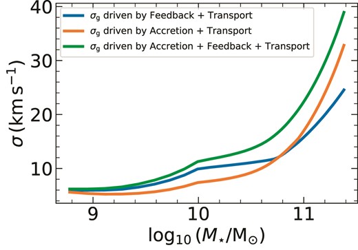
Gas velocity dispersion, σg, as a function of stellar mass, at z = 0. The three curves corresponds to models where turbulence is driven by either feedback due to star formation, gas accretion, gas transport, or a combination of the three.
Conversely, feedback plays a major role in driving turbulence in low-mass galaxies but becomes sub-dominant compared to accretion in massive galaxies. This is seemingly contrary to the findings of both KBFC18 and Ginzburg et al. (2022) who find that mass transport is the dominant driver of turbulence in massive local galaxies. However, KBFC18 did not consider accretion as a possible source of turbulence that would reduce the amount of transport needed to maintain σg, and Ginzburg et al. (2022) did not consider the GMC regime of star formation, which compared to their assumption that all galaxies are in the Toomre regime yields a higher |$\dot{M}_{\rm {sf}}$| and hence reduces the transport rate |$\dot{M}_{\rm {trans}}$| required to maintain energy equilibrium (cf. equation 7). Mass transport is thus very sensitive to model parameters that govern |$\dot{M}_{\rm {sf}}$| and ηw at z = 0. As we will discuss later, this has important consequences for the metallicity distribution and gradient in local galaxies.
2.2.1 Other potential drivers of turbulence
We pause here to briefly mention other potential sources of turbulence in the disc that we have not taken into account in this work.
Feedback from supermassive black holes is another potential source of turbulent energy injection in galaxies (e.g. Churazov et al. 2004; Zhuravleva et al. 2014; Li et al. 2020). For instance, both AGN-driven winds (Wagner, Umemura & Bicknell 2013) and radio jets (Mukherjee et al. 2018; Zovaro et al. 2019; Nesvadba et al. 2021) can enhance turbulence throughout the galactic disc on kpc scales. We also ignore turbulence injected by magnetorotational instabilities that could be important in the outskirts of galactic discs (Sellwood & Balbus 1999; Piontek & Ostriker 2005), since the current evidence remains rather inconclusive (Tamburro et al. 2009; Utomo, Blitz & Falgarone 2019; Bacchini et al. 2020).
Another class of potential turbulence drivers are stellar components of the galaxy that can transfer energy to the gas, for example, spiral arms and bars. While these can drive turbulence in the gas (Kim & Ostriker 2007; Haywood et al. 2016; Khoperskov et al. 2018; Orr et al. 2023), simulations spanning a variety of redshifts and halo masses find that they remain subdominant compared to feedback, transport, and accretion (Bournaud, Elmegreen & Elmegreen 2007; Bournaud & Elmegreen 2009; Ceverino, Dekel & Bournaud 2010; Goldbaum, Krumholz & Forbes 2015, 2016). Nevertheless, the impact of these drivers of turbulence on the gas-phase metallicity remains largely unexplored (e.g. Zurita et al. 2021; Chen et al. 2023a).
2.3 Evolution of gas-phase metallicity
The metallicity model of Sharda et al. (2021a) is a standalone model that uses a galaxy evolution model as an input to predict the metallicity profile in a wide variety of galaxies. The model includes several key physical processes – gas accretion, radial gas flows, metal advection and diffusion, star formation, metal consumption in long-lived stars, and outflows. In its primitive form, the evolution of spatially resolved gas-phase metallicity in this model is given by equation 14 of Sharda et al. (2021a):
where x and τ are the dimensionless galactocentric distance and time variables, respectively. x = r/r0, where |$r_0 = 1\, \rm {kpc}$| is the reference radius that we assume to be the inner edge of the disc. Similarly, |$\tau = t \, \Omega _0$|, where Ω0 is the angular velocity at r0. |$\mathcal {Z}$| is the gas-phase metallicity Z normalized to |$\rm {Z_{\odot }}$|. The parameters |$s_{\rm {g}} (x), k(x), \dot{s}_{\star }(x)$| and |$\dot{c}_{\star }(x)$|, respectively, represent the functional forms of spatial variations in the gas surface density Σg, epicyclic frequency κ, star formation rate surface density |$\dot{\Sigma }_{\star }$|, and gas accretion rate surface density |$\dot{\Sigma }_{\rm {g,acc}}$|.
We pause here to mention a key difference between our approach and that of Sharda et al. (2021a). These authors find sg(x) = 1/x, k(x) = x by assuming that vϕ is the same throughout the galactic disc. However, this is only valid as long as β ∼ 0. We further generalize their results by re-writing |$v_{\phi } = v_{\phi ,\rm {r}} (r/R)^{-\beta }$| where |$v_{\phi ,\rm {r}}$| is the rotational velocity at a distance r from the galaxy centre, and R is the disc size we define in equation (6). The advantage of re-writing the rotational velocity in this way is that we retain the meaning of vϕ as that defined at the outer edge of the disc. With this generalization, we obtain
It is expected that |$\dot{c}_{\star }$| declines with x (Chiappini, Matteucci & Romano 2001; Fu et al. 2009; Courty, Gibson & Teyssier 2010; Forbes et al. 2014b; Pezzulli & Fraternali 2016; Mollá et al. 2016; Stevens et al. 2017). We retain |$\dot{c}_{\star }(x)=1/x^2$| from Sharda et al. (2021a). While the motivation for such a radial variation in |$\dot{\Sigma }_{\rm {acc}}$| is that it can reproduce the present-day stellar surface density of the Milky Way (Colavitti, Matteucci & Murante 2008), there is no reason why all galaxies should follow this profile. Nevertheless, (appendix A Sharda et al. 2021a) show that a different functional form does not qualitatively change the resulting metallicity gradients in local spirals, and does not matter at all for local dwarfs, and we therefore adopt a single functional form for simplicity.
Since we include both the Toomre and the GMC regime of star formation, we update the definition of |$\dot{s}_{\star }$| such that it is a continuous function of x
where xb is the critical location in the disc where |$\dot{\Sigma }_{\star }$| in the GMC regime equals that in the Toomre regime (equation 32 of Krumholz et al. 2018)
Note that the star formation rate profile is less steep in the GMC regime, which will lead to more metal production in the outer regions of the galaxy as compared to the Toomre regime. As we will discuss later in Section 4, this feature is partially responsible for giving rise to steady-state inverted metallicity gradients in the model.
The four dimensionless ratios that connect the metallicity model to the evolution of gas and stars are: (1) |$\mathcal {T} -$| the ratio of the orbital and metal diffusion time-scales, (2) |$\mathcal {P} -$| the ratio of metal advection to metal diffusion, well known as the Péclet Number in fluid dynamics (Patankar 1980), (3) |$\mathcal {S} -$| the ratio of metal production (star formation) to metal diffusion, and (4) |$\mathcal {A} -$| the ratio of gas accretion to metal diffusion. As in Section 2.1, we have not taken into account the effect of galactic fountains in returning metals to the disc. As in equation (19) and equation (20a), we also generalize the expressions for |$\mathcal {T}, \mathcal {P}, \mathcal {S}$| and |$\mathcal {A}$| from Sharda et al. (2021a)
where xmax = R/r0 is the disc size normalized by r0, and ϕy is a fractional quantity that describes the preferential metal enrichment of galactic winds.6 Most galactic chemical evolution models to date assume that the metallicity of galactic winds is the same as that of the ISM. However, this is not necessarily the case for all galaxies. ϕy accounts for the fact that the wind metallicity can be higher than the ISM metallicity in a galaxy if the ejecta from supernovae are imperfectly mixed with the ISM (Dekel & Silk 1986; Mac Low & Ferrara 1999; Recchi et al. 2008; Peeples & Shankar 2011; Fu et al. 2013; Emerick et al. 2018; Emerick, Bryan & Mac Low 2019; Taylor, Kobayashi & Kewley 2020; Sharda et al. 2021a; Yates et al. 2021; Andersson et al. 2022), as has now been observed in galactic winds of low mass galaxies (Chisholm, Tremonti & Leitherer 2018; Lopez et al. 2020; Cameron et al. 2021; Xu et al. 2022; Tortora, Hunt & Ginolfi 2022). Following Sharda et al. (2021b, equation A1), we write
where y = 0.028 is the yield of newly formed Type II metals (Forbes, Krumholz & Speagle 2019) following the instantaneous recycling approximation (Tinsley 1980) and |$\mathcal {Z}_{\rm {w}}$| is the metallicity of galactic winds normalized to |$\rm {Z_{\odot }}$|. It is given by equation 41 of Forbes, Krumholz & Speagle (2019)
where fR,inst = 0.77 is the fraction of metals locked in low mass stars (Tinsley 1980), and ξw is a fractional parameter bounded between 0 and 1 that describes the preferential enrichment of galactic winds if some of the newly produced metals are ejected with winds before they mix with the ISM. Thus, equation (27) implies that common assumption of wind metallicity being equal to the ISM metallicity is likely only a lower bound in reality. Further, since a fraction fR,inst of metals are locked in stars, the minimum metal mass ejected is 1 − fR,inst.
We see from equation (26) that ϕy ∼ 0 corresponds to all newly produced metals being entrained in the winds, whereas if ϕy ∼ 1, newly produced metals are perfectly mixed with the ISM before they are ejected such that the wind metallicity equals the ISM metallicity. In the absence of any scaling relations of ϕy with galaxy properties, we explore ϕy in the range of 0.1−1, and show how the resulting metallicity gradients are quite sensitive to the choice of ϕy. In principle, we can specify ϕy as a spatially varying parameter. However, we treat it as an integrated quantity for this work since variations in ϕy with x remain unexplored. As we will discuss below, |$\mathcal {P}, \mathcal {S}$| and |$\mathcal {A}$| form the cornerstone of our metallicity analysis and act as useful diagnostics to understand what sets metallicity gradients in galaxies.
Note that we only consider elements produced by core collapse supernovae in this work, since the observable we study is the oxygen abundance gradient in the ISM. Therefore, we cannot comment on the evolution of ϕy for elements produced by other nucleosynthetic sources (e.g. AGB stars or Type Ia supernovae). In fact, simulations of low-mass galaxies that explicitly resolve feedback find metal enrichment of galactic winds to be dependent on the nucleosynthetic source (Emerick et al. 2018). Similarly, metal mixing in the ISM is also sensitive to the nucleosynthetic source (Krumholz & Ting 2018).
2.3.1 Metal equilibration time-scale
Because we are interested in searching for steady-state solutions to equation (18), we first estimate the time it takes for a given metal distribution to reach equilibrium, teqbm. Following Sharda et al. (2021a, equation 19), teqbm is given by
The physical interpretation of the above equation is that we compare the time taken by gas accretion, star formation, outflows, metal advection and metal diffusion to induce changes in metallicity with the rate at which metallicity evolves with time as given by the leading term in equation (18). Under equilibrium, |$\partial \mathcal {Z} / \partial \tau \rightarrow 0$|. This is a common practice in chemical evolution models, as it allows us to estimate if metallicity reaches equilibrium simultaneously with other galaxy properties (Davé, Finlator & Oppenheimer 2012; Lilly et al. 2013; Feldmann 2015; Krumholz & Ting 2018).
If the metal distribution does not reach equilibrium within a reasonable time, we consider the resulting gradients to be in non-equilibrium, in which case we cannot apply our model to study gradients. A necessary condition is that the metal equilibration time-scale be less than the Hubble time. However, this is not sufficient since physical processes relevant for the model may change on time-scales much shorter than the Hubble time. Out of all the physical processes we include, the time-scale for star formation, quantified by the molecular gas depletion time-scale, tdep, is usually observed to be the shortest (Genzel et al. 2015; Scoville et al. 2017; Utomo et al. 2017; Tacconi et al. 2018; Liu et al. 2019). In nearby galaxies, observations find |$t_{\rm {dep}} \approx 2\, \rm {Gyr}$| (Leroy et al. 2008; Bigiel et al. 2011; Saintonge et al. 2011; Sun et al. 2023). Keeping this in mind, we consider the metallicity to be in non-equilibrium if teqbm ≫ tdep. To ensure that local fluctuations in metallicity are not responsible for setting the metallicity gradient (that would otherwise generate a random metallicity gradient set by a stochastic metal field), we investigate if teqbm is longer than the time-scale for such fluctuations to become steady. Typically, the latter is of the order of |$t_{\rm {fluc}} \approx 300\, \rm {Myr}$| in local galaxies (fig. 7 of Krumholz & Ting 2018), and we check if teqbm ≳ tfluc. Given the self-consistent evolution of gas parameters with metals, the model we present here allows for inverted gradients to form in equilibrium, in contrast to the Sharda et al. (2021a) model.
2.3.2 Equilibrium solutions
Sharda et al. (2021a) show that most galaxies tend to achieve a steady-state metallicity gradient within a time-scale much shorter than the Hubble time, and comparable or shorter than tdep. When this condition is satisfied, we can search for equilibrium solutions for equation (18) by setting |$\partial \mathcal {Z} / \partial \tau \rightarrow 0$|.
Since the functional form of the star formation term, |$\dot{s}_{\star }(x)$|, is different in the Toomre and the GMC regimes of star formation, the resulting solution for |$\mathcal {Z}(x)$| is also different. |$\mathcal {Z}(x)$| in the Toomre regime is given by
and in the GMC regime is given by
Here, |$\mathcal {Z}_{r_0}$| is the metallicity at r0, and c1 is a constant of integration. Physically, c1 reflects the strength of the metallicity gradient at r0. Galaxies tend to achieve a particular value of |$\mathcal {Z}_{r_0}$| that is governed by the competition between terms that dominate at r0. For massive local galaxies, |$\mathcal {Z}_{r_0}$| is set by the competition between source (star formation and outflows) and accretion. For low-mass galaxies, |$\mathcal {Z}_{r_0}$| is set by the interplay between advection and diffusion if |$\dot{M}_{\rm {trans}} \gt 0$|. In the case where there is no mass transport (|$\dot{M}_{\rm {trans}} = 0$|), |$\mathcal {Z}_{r_0}$| is set by source and diffusion. We provide the equations for |$\mathcal {Z}_{r_0}$| in terms of c1 in Appendix C. Thus, c1 is the only unknown parameter in practice. We also see that equation (29) reduces to equation (41) of Sharda et al. (2021a) when β → 0.
With these solutions, we can develop some intuition for the steepness of the resulting metallicity profiles. If |$\mathcal {S} \gt \mathcal {P} + \mathcal {A}$|, the profiles are steeper, thus giving strong negative metallicity gradients. On the contrary, if |$\mathcal {P} + \mathcal {A} \gt \mathcal {S}$|, the metal distribution is quite homogeneous, giving flat metallicity gradients. In the extreme case where |$\mathcal {P} + \mathcal {A} \gg \mathcal {S}$|, this can even lead to an inversion in the metallicity profile where the inner regions of the galaxy are more metal-poor as compared to the outskirts, thereby driving an inverted metallicity gradient. The inversion is more likely to occur for low-mass galaxies because of the leading term that scales as xβ in both the Toomre and GMC regimes. The strength of the gradient is also modulated by c1, which we constrain using physically meaningful boundary conditions in Section 2.3.3.
2.3.3 Boundary conditions for equilibrium solutions
We follow Sharda et al. (2021a) to define boundary conditions for the equilibrium solutions we obtain in Section 2.3.2. These boundary conditions constrain c1 to a finite range of values that in turn give rise to a family of metallicity profiles (hence, gradients) for each solution. Note that if we excluded metal diffusion, equation (18) would reduce to first order, which will only have one constant of integration that can be fully specified using |$\mathcal {Z}_{r_0}$|. So, we would only obtain one profile per solution instead of a family of profiles.
We first require that |$\mathcal {Z}(x)$| is greater than some minimum value, |$\mathcal {Z}_{\rm {min}}$| at all x. This condition provides a lower bound on c1. We also demand that the metal flux crossing into the disc is at most equal to advection of metals from the CGM (with metallicity |$\mathcal {Z}_{\rm {CGM}}$|). Following Sharda et al. (2021a, equation 43), we express this condition as
This condition ensures that most metals present in the disc belong to the in situ population of metals produced by star formation (which is generally true unless galactic fountains recycle a significant amount of metals), and provides an upper bound on c1. We do not show the resulting equations for c1 here as they consist of several non-linear functions that are not illuminating, but they can be directly obtained by the applying the above constraints.
We set |$\mathcal {Z}_{\rm {CGM}} = 0.05$| for low-mass galaxies, 0.2 for massive galaxies, and create a linear ramp in log10M⋆ between these two for intermediate mass galaxies. Such a set-up roughly reproduces the metallicity of metal-poor inflows on to the disc seen in simulations (Muratov et al. 2017). As more measurements of |$\mathcal {Z}_{\rm {CGM}}$| become available (e.g. Prochaska et al. 2017; Kacprzak et al. 2019), it will be possible to refine the prescription we use.
This completes the formulation of the model. In Table 3, we provide a summary of key differences between our approach and earlier works we make use of.
| Parameter | KBFC18 | Sharda et al. (2021a) | Ginzburg et al. (2022) | This work |
|---|---|---|---|---|
| Evolution of |$\dot{M}_{\rm {g}}$| | ✕ | ✕ | ✓ | ✓ |
| Self-consistent |$\dot{M}_{\rm {g}}$| and σg | ✕ | ✕ | ✓ | ✓ |
| Radial resolution | ✕ | ✓ | ✕ | ✓ |
| Include GMC regime | ✓ | ✕ | ✕ | ✓ |
| Include ξa | ✕ | ✕ | ✓ | ✓ |
| Include σacc | ✕ | ✕ | ✓ | ✓ |
| Include ηw | ✕ | ✓ | ✕ | ✓ |
| Include |$\mathcal {Z}$| | ✕ | ✓ | ✕ | ✓ |
| Include ϕy | ✕ | ✓ | ✕ | ✓ |
| Include ϕa | ✓ | ✕ | ✕ | ✓ |
| Allow Q ≥ Qmin | ✓ | ✕ | ✕ | ✓ |
| Allow β ≠ 0 | ✓ | ✓ | ✕ | ✓ |
| Allow radial variations in vϕ | ✓ | ✕ | ✕ | ✓ |
| Allow ϕnt ≤ 1 | ✓ | ✕ | ✕ | ✓ |
| Allow fsf ≤ 1 | ✓ | ✓ | ✕ | ✓ |
3 EQUILIBRIUM METALLICITY GRADIENTS
We now present resulting ISM metallicity profiles and gradients from the model for two classes of galaxies. Table 4 lists the values of model parameters for the two representative galaxies. The top panel of Fig. 3 presents the resulting family of metallicity profiles from the model for a fiducial local massive galaxy with |$M_{\star } = 10^{10.8}\, \rm {M_{\odot }}$| at z = 0 with ϕy = 1.0 (solid curves) and 0.1 (dotted curves). We include all three sources of turbulence (feedback, accretion, and transport) to create these profiles. The family of curves results from the permissible range of values of the constant c1 in the metallicity equation. However, not all the gradients are in equilibrium. The colourbar in Fig. 3 informs on the time taken by the metal distribution to reach equilibrium compared to tdep; the redder the colour, the larger are the deviations from equilibrium. As expected, we see that the metallicity at the inner edge of the disc naturally approaches the value |$\mathcal {Z}_{r_0}$| set by the terms that dominate at small radii. The inner regions (x < 5) of all the profiles are in the Toomre regime of star formation whereas the outer regions are in the GMC regime, as expected from the KBFC18 model. The bottom panel of Fig. 3 presents the family of metallicity profiles for a fiducial local low-mass galaxy with |$M_{\star } = 10^{9}\, \rm {M_{\odot }}$|. In this case, the Toomre regime exists for x < 3.5, beyond which star formation occurs in GMCs. For the lowest mass galaxies we study, the entire star-forming disc is in the GMC regime at z = 0. For the massive galaxy, the radial metallicity profiles for high values of ϕy are consistent with the average metallicity profile observed in nearby galaxies of similar mass (Belfiore et al. 2017). On the other hand, model profiles with low values of ϕy in the low-mass galaxy better match the observed profiles for similar mass (see also Sharda et al. 2021a, figs 2 and 5).

Top panel: ISM metallicity profiles (|$\mathcal {Z} = Z/Z_{\odot }$|) as a function of the dimensionless radius (x = r/r0 with |$r_0 = 1\, \rm {kpc}$|) for the fiducial case of a massive galaxy (|$M_{\star } = 10^{10.8}\, \rm {M_{\odot }}$|) with ϕy = 1.0 (solid) and 0.1(dotted), respectively. ϕy describes the preferential metal enrichment of galactic winds. The family of curves for each ϕy arise from constraints on the constant of integration c1 in the solution for metallicity. Colourbar represents the difference between the metal equilibration time-scale, teqbm, and the gas depletion time-scale, tdep, with increasingly red colour representing larger deviations from equilibrium. Bottom panel: Same as the top panel but for a low-mass galaxy with |$M_{\star } = 10^{9}\, \rm {M_{\odot }}$|.
List of parameter values for metallicity gradients in two representative galaxies as shown in Fig. 3.
| Parameter | Massive galaxy | Low-mass galaxy |
|---|---|---|
| M⋆ | |$10^{10.8}\, \rm {M_{\odot }}$| | |$10^{9}\, \rm {M_{\odot }}$| |
| xmax | 15 | 5.5 |
| fg, Q | 0.5 | 0.9 |
| ϵin | 0.24 | 0.46 |
| c | 10 | 15 |
| β | 0 | 0.5 |
| fsf | 0.6 | 0.4 |
| fg, P | 0.5 | 0.9 |
| Parameter | Massive galaxy | Low-mass galaxy |
|---|---|---|
| M⋆ | |$10^{10.8}\, \rm {M_{\odot }}$| | |$10^{9}\, \rm {M_{\odot }}$| |
| xmax | 15 | 5.5 |
| fg, Q | 0.5 | 0.9 |
| ϵin | 0.24 | 0.46 |
| c | 10 | 15 |
| β | 0 | 0.5 |
| fsf | 0.6 | 0.4 |
| fg, P | 0.5 | 0.9 |
To find a 1D gradient, we fit the logarithmic metallicity profiles with a linear function in x from 1 to xmax (see Table 4), the slope of which is the metallicity gradient. This is an oversimplification because the profiles are typically more complex given the non-linearity of |$\mathcal {Z}(x)$|, so a gradient returned by the fit is often a poor representation of the underlying profile. However, we use this approach to mimic observational measurements where the 2D maps are reduced to 1D by stacking metallicity profiles as a function of galactocentric distance, and then fit with a linear function in |$\log _{10} \mathcal {Z}$|. For the massive galaxy, we find gradients to be in the range |$-0.18\, \mathrm{dex}\, r^{-1}_{\rm {e}}$| to |$0.08\, \mathrm{dex}\, r^{-1}_{\rm {e}}$|, where we take re ≈ R/2 in the model; adopting re from van der Wel et al. (2014) (as in Sharda et al. 2021a) gives similar results. Similarly, we obtain gradients in the range |$-0.23\, \mathrm{dex}\, r^{-1}_{\rm {e}}$| to |$0.13\, \mathrm{dex}\, r^{-1}_{\rm {e}}$| for the low-mass galaxy. Typically, profiles given by the maximum possible value of c1 (especially for massive galaxies) are out of equilibrium, and these profiles lead to inverted gradients. While most inverted metallicity gradients are out of equilibrium in the model, we do find some steady-state profiles where the metallicity in the outer regions is larger than that in the inner regions. This differs from our earlier models in Sharda et al. (2021a), which did not include the GMC regime of star formation and did not find any inverted gradient equilibria.
Given this new finding, it is worth investigating how these inverted gradients form and exist in equilibrium. Let us consider a simpler case of a massive galaxy with no advection, so |$\beta = \mathcal {P} = 0$|. In such a case, at large radii, accretion and diffusion compete with star formation to set the metallicity. However, star formation in the GMC regime only declines with radius as 1/x, while accretion and diffusion go as 1/x2. So, even though fewer metals are being produced at large radii, the rate at which they are diluted or transported is even smaller. This is why metallicity in the outskirts can be higher, leading to inverted gradients in the model in equilibrium. However, there are two important corollaries. First, this result is sensitive to our assumed radial profile of accretion, |$\dot{c}_{\star } = 1/x^2$| (Colavitti, Matteucci & Murante 2008). If we assume that accretion goes as 1/x instead, for example, the resulting gradient will likely be close to zero. Second, if fsf declines strongly with radius (e.g. Krumholz, McKee & Tumlinson 2009; Krumholz 2013; Kubryk, Prantzos & Athanassoula 2015), the source term |$\mathcal {S}$| would decrease more rapidly than 1/x, and we would again have no or less inversion. We also do not invoke radial variations in ϕy or ηw below (e.g. Johnson et al. 2021). Exploring radial variations in these parameters requires direct measurements of both the molecular and atomic gas surface densities, as well as metal enrichment of galactic winds at different radii. This is an area where a multiwavelength observations, combining JWST IFU instruments, VLT/MUSE and ALMA (e.g. Leroy et al. 2021; Emsellem et al. 2022) have the potential to make a big impact on our understanding of inverted metallicity gradients.
Note that our model is based on a disc flow model, but (major) mergers can significantly impact the disc, and likely reset the metallicity gradients. We showed in Sharda et al. (2021a) that the metallicity distribution falls out of equilibrium during a major merger (a result corroborated by observations – Pérez-Díaz et al. 2023), and thus our equilibrium model cannot be applied in such cases. It is for this reason that we do not study merging galaxies (e.g. ULIRGs) in this work. The impact of minor mergers is small at resetting the gas-phase metallicity gradient, especially at z = 0, which is the focus of this work. There is an associated question of the impact of past major mergers on the present day metallicity gradient in the disc, answering which requires using a combination of hydrodynamic simulations and SAMs like ours (Sharda et al., in preparation), and is beyond the scope of this work.
4 MZGR WITH THE FIDUCIAL MODEL
We show the observed MZGR (corrected for spatial resolution) from three different surveys – MaNGA (Mapping Nearby Galaxies at Apache Point Observatory, Bundy et al. 2015), CALIFA (Calar Alto Legacy Integral Field Area, Sánchez et al. 2012), and SAMI (Sydney-AAO Multi-object Integral-field spectrograph, Bryant et al. 2015) in Fig. 4. Each marker denotes the average metallicity gradient (normalized by re) in different bins of stellar mass. It is immediately clear that even between the three surveys, average gradients differ by as much as |$0.1\, \mathrm{dex\, }r^{-1}_{\rm {e}}$|. In fact, the galaxy-to-galaxy scatter at fixed M⋆ is as high as |$0.3\, \mathrm{dex\, }r^{-1}_{\rm {e}}$|. The scatter is larger at the low- and high-mass ends than at intermediate masses (fig. 10 of Poetrodjojo et al. 2021). While some of this scatter can be physical (especially at the low-mass end), it is also caused by systematic differences between gas-phase metallicity calibrations (Kewley & Ellison 2008), limited spatial resolution and S/N ratio (Mast et al. 2014; Acharyya et al. 2020), the sensitivity of metallicity diagnostics to physical properties of H ii regions such as ionization parameter (e.g. Pettini & Pagel 2004; Kobulnicky & Kewley 2004; Pilyugin & Grebel 2016; Curti et al. 2017; Mingozzi et al. 2020), and to poorly understood contributions from diffuse ionized gas (DIG; Sanders et al. 2017; Zhang et al. 2017; Poetrodjojo et al. 2019; Vale Asari et al. 2019). An important effect of this discrepancy is that it is not clear if the MZGR shows an inflection at |$9.5 \lt \log _{10} M_{\star }/\rm {M_{\odot }} \lt 10.5$| (Belfiore et al. 2017; Mingozzi et al. 2020); some studies favour such a break whereas others find a constant, characteristic gradient for all galaxies (Sánchez et al. 2014; Sánchez-Menguiano et al. 2016, 2018; Poetrodjojo et al. 2018).
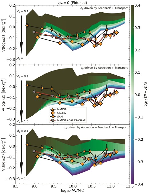
The local MZGR as predicted from the fiducial model. It plots metallicity gradients (|$\nabla \log _{10}\, \mathcal {Z}$|) as a function of the stellar mass (M⋆). The colourbar indicates the ratio of the strength of processes that create flat metal distributions (|$\mathcal {P}$| and |$\mathcal {A}$|) to those that create steep metallicity gradients (|$\mathcal {S}$|) in equilibrium, as defined in Section 2. The top panel plots the model MZGR for the case where only gas accretion and transport drive turbulence in the galaxy. The middle panel corresponds to the case where only star formation feedback and gas transport drive turbulence. The bottom panel corresponds to the case where all three factors are included as drivers of gas turbulence. The scatter in the model at fixed M⋆ corresponds to the results of varying ϕy, the parameter that describes the preferential ejection of metals via galactic winds, from 0.1 to 1, as indicated. Overplotted (orange markers) are average metallicity gradients in bins of M⋆ obtained from IFU surveys – MaNGA (Belfiore et al. 2017; Mingozzi et al. 2020), CALIFA (Sánchez et al. 2014; Sánchez-Menguiano et al. 2016), and SAMI (Poetrodjojo et al. 2018), as well as mean of the three (grey markers).
Using the second data release of SAMI data, Poetrodjojo et al. (2021) reduce the discrepancy due to different emission line ratios and metallicity calibrations to |$0.02\, \mathrm{dex\, }r^{-1}_{\rm {e}}$| by using a carefully chosen combination of various diagnostics that include more than two emission line ratios (e.g. Pilyugin & Grebel 2016). These authors find that there is indeed evidence for a break in the MZGR between |$9.5 \lt \log _{10} M_{\star }/\rm {M_{\odot }} \lt 10.5$|, however, the feature is rather weak as compared to the curvature observed in the MZR. Franchetto et al. (2021) reach the same conclusion based on their analysis of the MZGR in the MaNGA and GASP (GAs Stripping Phenomena in galaxies with MUSE, Poggianti et al. 2017) surveys. Deciphering the origin of the MZGR and determining whether there is an inflection at intermediate masses is important to understanding how various physical processes we describe in Section 2 impact metal distribution in galaxies.
To construct an MZGR from our model, we specify a range of halo masses at high-z such that the resulting halo mass at z = 0 span |$10.9 \lt \log _{10} M_{\rm {h}}/\rm {M_{\odot }} \lt 14$|.7 As we saw in Section 3, the model produces a family of metallicity profiles. Below, we find the MZGR for different cases corresponding to the different drivers of turbulence (feedback, accretion, and transport).
4.1 Gas turbulence driven by feedback and transport
In this case, the Péclet number |$\mathcal {P}$| that describes the ratio of metal advection to diffusion is set only by star formation feedback and gas transport (σg corresponding to the blue curve in Fig. 2). This is the case studied in Sharda et al. (2021a) since the KBFC18 model we used only considers feedback and transport as sources of turbulence. However, there are several differences between this and earlier work, as we point out in Section 2.
The top panel of Fig. 4 plots the resulting MZGR from the model in this case. We colour code the model MZGR by the ratio |$(\mathcal {P} + \mathcal {A}) /\mathcal {S}$|; the reason for this coding is that the processes parametrized by the numerator (advection and accretion) tend to flatten the gradient, while the one parametrized by the denominator (star formation) tends to steepen it. Thus this ratio is effectively the ratio of flattening to steepening processes. We show the resulting values of |$\mathcal {P}$|, |$\mathcal {A}$|, and |$\mathcal {S}$| for this case in the left-hand panel of Fig. 5. The scatter in |$\mathcal {S}$| at fixed M⋆ is caused by ϕy (see equation 24). In line with our expectations, we see that steep negative gradients develop when |$\mathcal {S} \gt \mathcal {P} + \mathcal {A}$|; this process is largely controlled by the parameter ϕy, since at fixed M⋆ increasing ϕy leads to larger |$\mathcal {S}$| (as indicated by colour in Fig. 4) and to steeper, negative gradients (corresponding to moving downward in Fig. 4). The exception to this trend is the least massive galaxies with |$M_{\star } \lt 10^{9.1}\, \rm {M_{\odot }}$| – these galaxies lie in the GMC regime of star formation, as against galaxies with |$M_{\star } \ge 10^{9.1}\, \rm {M_{\odot }}$| where the inner regions are in the Toomre regime and the outer regions are in the GMC regime. Since the star formation time-scale is capped by tSF,max in the GMC regime, the resulting |$\mathcal {S} \lt \mathcal {P} + \mathcal {A}$| even with ϕy = 1, as we can also read off from the left panel of Fig. 5. We also find that |$\mathcal {A} \gt 1$| for all M⋆ in this case, implying that metal diffusion is weak as compared to gas accretion. However, metal diffusion dominates over metal advection and star formation in some low-mass galaxies that have |$\mathcal {P} \lt 1$| and |$\mathcal {S} \lt 1$|. Since diffusion tends to homogenize the metal distribution by moving metals from high to low concentrations, strong diffusion leads to flatter gradients. The inflection we see in the MZGR at |$M_{\star } \approx 10^{9.2}\, \rm {M_{\odot }}$| occurs due to mass transport shutting off.
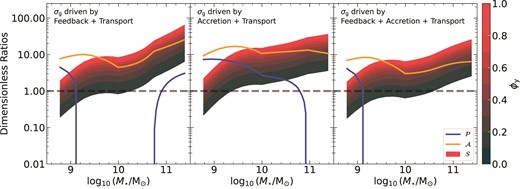
Left panel: The three dimensionless ratios (|$\mathcal {P}, \mathcal {A}$|, and |$\mathcal {S}$|) that set the metal distribution at z = 0 in the fiducial model presented in Section 4, as a function of stellar mass, for the case where turbulence is driven by star formation feedback and gas transport. The value of |$\mathcal {S}$| is directly proportional to the parameter ϕy that describes the preferential enrichment of galactic winds (see equation 24), so for this parameter we plot a vertical range corresponding to varying ϕy from 0.1 to 1, as indicated by the colourbar. Metal transport due to radial gas flows (|$\mathcal {P}$|) is only active for the lowest and most massive galaxies in this case. The dashed line denotes a value of unity, with values of a parameter less than unity indicating that turbulent diffusion is a more important process than the one described by that parameter. Middle panel: Same as the left panel but now turbulence is driven by gas accretion and transport. Metal advection is active for most galaxies in this case. Right panel: Same as the other two panels but turbulence is now driven by all three mechanisms – feedback, accretion, and transport. Metal advection is active only in the lowest mass galaxies. These diagnostic plots aid in understanding the nature of metal distributions and metallicity gradients in each of the corresponding models presented in Fig. 4.
We further see that there is a large scatter in the gradient at fixed stellar mass (especially in low-mass galaxies) that narrows at the high-mass end. This scatter occurs because the gradients are quite sensitive to the choice of ϕy–low ϕy lowers |$\mathcal {S}$|, driving flat or even inverted gradients, whereas high ϕy drives steep negative gradients. At the low-mass end, the data prefers low values of ϕy, implying a significant boost in preferential metal ejection in winds of low-mass galaxies. In the absence of accretion as a source of turbulence, σg equilibrates to a lower value that is closer or equal to σSF. This in turn causes |$\mathcal {P}$| to go to zero, thus shutting off mass transport and driving flatter (and even inverted) metallicity gradients at the high-mass end. This is complimented by the dramatic increase in |$\mathcal {S}$| and an even larger increase in |$\mathcal {A}$| because |$\mathcal {S} \propto \sigma ^2_{\rm {g}}$| and |$\mathcal {A} \propto \sigma ^3_{\rm {g}}$|. We find that this model fails to reproduce the observed MZGR, especially at the high-mass end.
At first look, this result seems contradictory to the MZGR presented in Sharda et al. (2021b), because these authors could also reproduce the high-mass end of the observed MZGR with just feedback + transport. However, their ad-hoc choice of σg was larger than that we derive in this work (blue curve in Fig. 2). Larger σg led to |$\mathcal {P} \gt 0$| and smaller |$\mathcal {A}$| in massive galaxies in Sharda et al. (2021b), yielding flatter gradients in good agreement with those observed. As we will discuss below, our self-consistent solution for σg that includes accretion as a source of turbulence does reproduce the MZGR at the high-mass end because of larger σg. This highlights the importance of accretion and turbulence in setting ISM metallicity distributions and gradients in massive galaxies.
4.2 Gas turbulence driven by accretion and transport
Next, we discuss the case where gas turbulence is driven by a combination of accretion and transport (orange curve in Fig. 2). We show the predictions from the model in the middle panel of Fig. 4, and the corresponding dimensionless ratios in the middle panel of Fig. 5. Overall, this model produces flatter metallicity gradients as compared to the feedback + transport model in Section 4.2. It can also reproduce the diversity of metallicity gradients in low-mass galaxies, although the range of ϕy that best matches the data is narrower as compared in the feedback + transport case. Including accretion as a source of turbulence brings the model gradients closer to the data, but agreement is still quite poor for massive galaxies. This is because |$\mathcal {P} \gt 1$| in most galaxies where transport is active, so a combination of strong metal advection and relatively higher gas accretion drives the flat and inverted gradients in this model. Thus, we learn that removing feedback and accretion as sources of turbulence results in model gradients that are too flat or inverted at the high-mass end as compared to the observed MZGR.
4.3 Gas turbulence driven by accretion, feedback, and transport
We have seen that if feedback and accretion are not included as sources of turbulence in the disc, the resulting model MZGRs do not reproduce the observed MZGR at the high-mass end, even with the uncertainty in ϕy. Now, we consider the more general case where σg is driven by feedback, accretion, and transport acting together (the green curve in Fig. 2). The bottom panel of Fig. 4 plots the model MZGR with the data. We find that the agreement between the model and the data is much better at all M⋆ as compared to the cases above where we exclude either feedback or accretion as sources of turbulence. Higher σg caused by turbulence due to all three sources (under energy balance) leads to smaller |$\mathcal {S}$| and even smaller |$\mathcal {A}$| that results in steeper gradients, particularly at the high-mass end. We can also discern the same from the right panel of Fig. 5. As compared to the other two models, we see that |$\mathcal {A}$| is smaller due to larger σg. The inflection in the MZGR at |$M_{\star } \approx 10^{9.2}\, \rm {M_{\odot }}$| that we noticed in the feedback + transport model is also present in this case, due to |$\mathcal {P} \rightarrow 0$| as mass transport shuts off. In equilibrium, the strength of mass transport is very sensitive to |$\dot{M}_{\rm {sf}}$| at z = 0, and thus to variations in the star-forming gas fraction fsf to which |$\dot{M}_{\rm {sf}}$| is proportional. We explore alternate models of fsf in Appendix A and show that the model MZGR at the high-mass end (where transport may or may not be shut off) remains qualitatively similar.
We also see that low-mass galaxies strongly prefer a low ϕy, implying significant metal enrichment of galactic winds. Below, we will see that this conclusion holds irrespective of the mass-loading of galactic winds in low-mass galaxies. We remind the reader that we adopt ξa = 0.2 for local galaxies, and show in Appendix B how the results change in the unlikely case where ξa is higher. As we show in Appendix D using MaNGA data, these interpretations are robust to scatter caused by different metallicity diagnostics used to measure metallicity gradients in the data (see also Poetrodjojo et al. 2021; Sharda et al. 2021a).
5 ROLE OF GALACTIC WINDS
As we mention in Section 2.1.4, the fiducial model we have presented so far is limited, and to some extent, inconsistent, because we include mass-loading of galactic winds (ηw) in the evolution of metallicity (cf. equation 27) but not in the evolution of the gas mass. There are several different scalings of ηw available in the literature, which can broadly be grouped into two categories: one where ηw is related to the large-scale properties of the galaxy (e.g. Mh and virial velocity, Murray, Quataert & Thompson 2005; Muratov et al. 2015; Pillepich et al. 2018a; Mitchell et al. 2020a; Pandya et al. 2021), and another where it is described by properties internal to the disc (e.g. Σg, ΣSFR, and fg; Dekel & Krumholz 2013; Hayward & Hopkins 2017; Kim et al. 2020; Pandya et al. 2021; Bassini et al. 2023). To rectify the inconsistency between metals and the gas, we discuss three cases below where we adopt ηw from the two groups of works as above. Our choice of adopted models is such that we can cover a broad range in ηw at fixed M⋆. While this approach of adopting ηw from other works still renders the treatment of outflows decoupled from the rest of the model, the advantage of using these recipes is that they can easily be incorporated into semi-analytical models like ours.
5.1 Effects of different mass loading parametrizations
- Mass-loading factor from Hayward & Hopkins (2017). Using an analytical model that describes the dual role of star formation feedback in regulating star formation as well as launching winds from the galactic disc, Hayward & Hopkins (2017) show that the gas fraction is a critical factor that determines ηw in star-forming galaxies. These authors find that gas-rich galaxies are typically more turbulent, and turbulence causes sharper density contrasts in the ISM (e.g. Federrath et al. 2010; Federrath & Klessen 2012; Burkhart 2018). As a result, low-density material is more efficiently accelerated out of the disc by star formation feedback. We adopt the approximate relation between the gas fraction, fg, HH17, and ηw provided by Hayward & Hopkins that effectively captures their detailed calculations(32)$$\begin{eqnarray} \eta _{\rm {w}} = 14 \left(f_{\rm {g,HH17}} \frac{M_{\star }}{10^{10} \rm {M_{\odot }}}\right)^{-0.23} e^{-0.75/f_{\rm {g,HH17}}}\, , \end{eqnarray}$$where fg, HH17 = Mg/(Mg + M⋆) is given by Hopkins et al. (2009, 2010):(33)$$\begin{eqnarray} && {f_{\rm {g,HH17}} = f_{\rm {0,HH17}} \left[1 - \tau (z)\left(1 - f^{3/2}_{\rm {0,HH17}}\right)\right]^{-2/3} } \\ && f_{\rm {0,HH17}} = \left[1 + \left(\frac{M_{\star }}{10^{9.15}\, \rm {M_{\odot }}}\right)^{0.4}\right]^{-1}\, , \end{eqnarray}$$
where τ(z) is the fractional redshift given by the ratio of lookback time at given z to that at z → ∞. However, this model uses a scaling |$\Sigma _{\rm {SFR}} \propto \Sigma ^{1.7-2}_{\rm {g}}$| (Faucher-Giguère, Quataert & Hopkins 2013; Thompson & Krumholz 2016) that is too steep as compared to the well-known Kennicutt-Schmidt relation (Kennicutt 1998).
- Mass-loading factor from FIRE-2 simulations. We use the best-fitting scaling of the multi-phase ISM ηw (measured in a radial shell between |$0.1-0.2\, R_{\rm {vir}}$|) as a function of M⋆ from FIRE-2 zoom-in simulations (Hopkins et al. 2018):(34)$$\begin{eqnarray} \eta _{\rm {w}} = 10^{4.3} \left(\frac{M_{\star }}{\rm {M_{\odot }}}\right)^{-0.45}\, . \end{eqnarray}$$
This scaling is based on an analysis of multiphase winds in central galaxies of 13 haloes spanning a wide range of Mh (equation 15 of Pandya et al. 2021). A key improvement over similar studies is that Pandya et al. define a more physically meaningful criteria to define outflowing gas particles that also encaptures the slow-moving hot wind. However, the set of simulations used for this analysis does not include AGN feedback and turbulent metal diffusion.
Mass-loading factor from EAGLE simulations: Lastly, we adopt the relation between ηw measured in EAGLE galaxies (Schaye et al. 2015) as a function of M⋆ from Mitchell et al. (2020a, fig. 15). Similar to Pandya et al. (2021), this ηw corresponds to mass leaving the ISM of the galaxy, and not the halo, and is measured for central galaxies. Crucially, the simulations used for this work by Mitchell et al. include AGN feedback. However, the criteria used by EAGLE to select outflowing gas particles is different than FIRE-2 (see section 2.6 of Mitchell et al. 2020a).
These scalings of ηw also constrain the range over which ϕy can vary, as against the fiducial model where we swept across ϕy = 0−1. This is simply because a fixed value of ηw limits the range of ξw in equation (27) that in turn limits ϕy. However, as we can expect from equation (27), this constraint is only used in practice in galaxies where ηw < 1 − fR,inst.
Fig. 6 unifies these scaling relations to represent them as a function of M⋆ for illustration. We find that, at the low-mass end, ηw from all the three works are qualitatively consistent with each other. While different simulations qualitatively agree on the behaviour of ηw with M⋆ for low-mass galaxies, they do not converge on the partition of mass and metal loading in the different phases of galactic winds as this is sensitive to the distance from the mid-plane where ηw is measured. There also exists tension between ηw measured in simulations and observations (e.g. Concas et al. 2022; Marasco et al. 2023). Simulations of isolated galaxies that can afford very high resolution tend to measure mass fluxes few |$\rm {kpc}$| from the mid-plane (e.g. Kim et al. 2020; Vijayan et al. 2020; Wibking & Krumholz 2022), whereas cosmological simulations tend to measure much farther away from the disc (see the discussion in Pandya et al. 2021). However, there is a large scatter in ηw for simulated massive galaxies. The key reason for this difference is that EAGLE includes AGN feedback that boosts mass-loading in massive galaxies at z = 0. In the absence of AGN feedback, it is difficult to drive strong winds in massive galaxies due to their deep potential wells. While our model does not include AGN feedback and is closer in spirit to Hayward & Hopkins (2017), it is insightful to test how AGN feedback-dominated ηw impacts the MZGR.
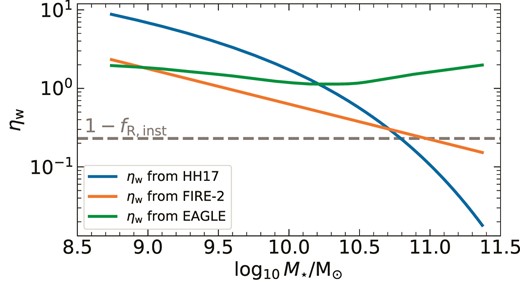
Mass loading factor, ηw, as a function of stellar mass at z = 0 from the three different cases we consider: (1) analytical model for star formation-driven winds (blue, Hayward & Hopkins 2017), (2) FIRE-2 cosmological zoom-in simulations without AGN feedback (orange, Pandya et al. 2021), and (3) EAGLE cosmological simulations including AGN feedback (green, Mitchell et al. 2020a). The dashed grey line demarcates 1 − fR,inst, the fraction of newly formed metals not locked in low-mass stars (Tinsley 1980).
5.2 Results
We know from equation (7) that introducing ηw ≠ 0 activates the outflow sink term that takes mass out of the disc and thus impacts Mg. Since σg ∝ Mg, and the dimensionless ratios that govern the metallicity profile are all sensitive to σg, we expect wind mass loading to non-linearly modulate the metallicity profiles and resulting metallicity gradients. Figs 7–9 plot the resulting model MZGR where we scale ηw following Hayward & Hopkins (2017), Pandya et al. (2021), and Mitchell et al. (2020a), respectively. We only plot the model for the case where turbulence is driven by a combination of feedback, accretion, and transport, as we have seen in Section 4 that neglecting either feedback- or accretion-driven turbulence does not reproduce the observed MZGR even in the fiducial case with ηw undefined.

We first discuss results for the scaling of ηw from Hayward & Hopkins (2017). We notice from Fig. 7 that, as compared to the fiducial model (bottom panel of Fig. 4), the range of metallicity gradients at the high-mass end of the MZGR remains unaffected by this scaling. This is because even at fixed ϕy, the model produces a family of gradients due to constraints on c1 (see Section 2.3.3). However, the range of gradients at the low-mass end is reduced by more than |$0.1\, \rm {dex}\, r^{-1}_{\rm {e}}$|, due to a high ηw > 1 for low-mass galaxies. While this scaling of ηw can capture the observed MZGR, the mechanism giving rise to the agreement between the observations and the model is significantly different as compared to the fiducial model, as we see from the differences in the ratio |$(\mathcal {P} + \mathcal {A})/\mathcal {S}$| denoted by the colourbar. The transition in colour from green to blue as a function of increasing M⋆ implies a transition in the dominant mechanism that sets metallicity gradients in low-mass versus massive galaxies, and is responsible for driving the model MZGR. Additionally, the best match between the model and the data reveals a large scatter in the preferred value of ϕy for galaxies with |$M_{\star } \lt 10^{9.4}\, \rm {M_{\odot }}$|: low-mass galaxies in the SAMI survey prefer ϕy ∼ 0.1, whereas MaNGA and CALIFA dwarfs prefer ϕy ∼ 0.4. The average measurement for the three surveys prefers ϕy ∼ 0.25. Massive galaxies (|$M_{\star } \gtrsim 10^{10}\, \rm {M_{\odot }}$|) prefer ϕy ∼ 0.8−1.0.
To further diagnose the cause for these differences, we plot the dimensionless ratios as a function of M⋆ for this scaling in the left panel of Fig. 10. At the high-mass end, ϕy is restricted to a very narrow range close to unity because ηw in the Hayward & Hopkins model is less than 1 − fR, inst, which limits the allowed range of |$\mathcal {Z}_{\rm {w}}$| (cf. equation 27). Physically, we can understand this result very simply: for these galaxies the mass flux carried by the winds is so small that, even if this mass were to consist of pure SN ejecta, winds would carry away at most a small fraction of the metals being produced. Thus most metals must remain in the galaxy, corresponding to ϕy close to unity. Since the dimensionless ratio |$\mathcal {S} \propto \phi _{\rm {y}}$|, this leads to a decrease in the quantity |$(\mathcal {P} + \mathcal {A})/\mathcal {S}$|, which in turn drives the colourbar to blue at the high-mass end in Fig. 7. We also see from the left panel of Fig. 10 that |$\mathcal {P} \gt 0$| only for galaxies with |$M_{\star } \lt 10^{10}\, \rm {M_{\odot }}$|, implying that mass transport shuts off in massive galaxies because accretion and feedback can drive sufficient levels of turbulence in these galaxies. Lastly, metal diffusion dominates over star formation for a wider range of M⋆ in this case as compared to the fiducial model.
Next, we examine the MZGR using the scaling of ηw from FIRE-2 zoom-in simulations. Fig. 8 shows the results. The scatter in metallicity gradients at the low mass end is larger than both the fiducial model and the model above where ηw scales according to the Hayward & Hopkins model. This correlates with the non-zero |$\mathcal {P}$| as we show in the middle panel of Fig. 10, and occurs because ηw measured in FIRE-2 dwarf galaxies is smaller by almost an order of magnitude as compared to Hayward & Hopkins. On the contrary, the scatter at the high-mass end remains identical to the other models, although the relative contribution of the dimensionless ratio |$\mathcal {S}$| is larger than the fiducial model but smaller than the model with ηw from Hayward & Hopkins. This occurs because the larger ηw in FIRE-2, as compared to Hayward & Hopkins, leads to a wider range of ϕy, as we read off from the middle panel of Fig. 10. Nevertheless, ηw from FIRE-2 simulations also results in an MZGR that can reproduce the observed data, but the preferred value of ϕy for low-mass galaxies is lower as compared to the case above with ηw from Hayward & Hopkins. Specifically, models with ϕy ∼ 0.1−0.2 best reproduce metallicity gradients in low-mass galaxies in all the three IFU surveys in this case. The preferred values of ϕy for massive galaxies remain similar to the case above.

Finally, we examine the case where we scale ηw following the EAGLE simulations (Mitchell et al. 2020a). We plot the resulting model MZGR in Fig. 9, and the corresponding diagnostic plot for the dimensionless ratios in the right panel of Fig. 10. For |$10^{9}\, \mathrm{M_{\odot }} \lt M_{\star } \lt 10^{10.7}\, \mathrm{M_{\odot }}$|, the MZGR from EAGLE is similar to that we obtain from FIRE-2 results above. The difference in the range of gradients at |$M_{\star } \lt 10^{9}\, \mathrm{M_{\odot }}$| between the two is due to a non-zero |$\mathcal {P}$| in FIRE-2. Further, the best match between the observed and the EAGLE MZGR also leads to ϕy ∼ 0.1−0.2 for low-mass galaxies. This is not surprising given ηw from both these simulations for low- and intermediate-mass galaxies is within a factor of few (Fig. 6). While the range of metallicity gradients predicted for massive galaxies is also the same, the underlying mechanism is qualitatively different. As compared to Fig. 8, we see that |$(\mathcal {P}+\mathcal {A}) \gt \mathcal {S}$| for some gradients at large M⋆. The reason behind this is the fact that EAGLE includes AGN feedback that boosts ηw above 1 − fR,inst for massive galaxies. As a consequence, EAGLE allows ϕy to be as low as possible, which in turn decreases |$\mathcal {S}$|. We confirm this from the range of ϕy and |$\mathcal {S}$| we observe from the right panel of Fig. 10.

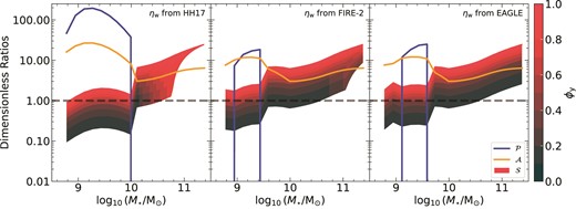
Left panel: Strength of the dimensionless ratios in the metallicity model (|$\mathcal {P}, \mathcal {A}$|, and |$\mathcal {S}$|) as a function of M⋆ for the case where turbulence is driven by feedback, accretion, and transport, and the mass-loading factor, ηw, scales with the gas fraction and M⋆, following an analytical model of star formation-driven winds (Hayward & Hopkins 2017). Colourbar denotes the permitted range of ϕy that describes the preferential enrichment of galactic winds (see equation 26). Middle panel: Same as the left panel but ηw is scaled with M⋆ following FIRE-2 cosmological zoom-in simulations without AGN feedback (Pandya et al. 2021). Right panel: Same as the other two panels but ηw is scaled with M⋆ following EAGLE cosmological simulations that include AGN feedback (Mitchell et al. 2020a).
We can summarize the overall conclusions from using different scalings of ηw as follows: (1) there is a transition in the dominant process setting metallicity gradients in local galaxies as a function of M⋆; gradients are set by |$\mathcal {P}$| (advection) and |$\mathcal {A}$| (accretion) in low-mass galaxies, and |$\mathcal {S}$| (production) begins to play an important role in setting the gradients in intermediate-mass and massive galaxies, (2) discrepancies in ηw that exist for massive galaxies due to AGN feedback lead to different mechanisms setting the high-mass end of the MZGR, (3) mass-loading is less critical for the MZGR as compared to metal-loading, and (4) low-mass galaxies seem to prefer a low ϕy irrespective of our adopted scaling of ηw, implying winds in low-mass galaxies are metal-enriched compared to their ISMs.
5.3 Predicted scaling of metal enrichment of galactic winds
Based on this analysis, we can now predict a scaling of ϕy that describes the preferential metal enrichment of galactic winds using ηw from the three studies we discuss above in Section 5.2. Such an exercise is similar in spirit to Peeples & Shankar (2011) who predict the scaling of the ratio |$\mathcal {Z}_{\rm {w}}/\mathcal {Z}$| based on the best match between their chemical evolution model and the MZR from Sloan Digital Sky Survey (SDSS; Tremonti et al. 2004). For this purpose, we use the observed MZGR from the three IFU surveys as well as their overall mean, and calculate the range of ϕy needed to reproduce the average metallicity gradient observed per M⋆ in the model with ηw from Hayward & Hopkins (2017), Pandya et al. (2021), and Mitchell et al. (2020a). Specifically, we start with a uniform distribution of ϕy from 0 to 1; for each ϕy, we check if the model in question can reproduce the gradients observed in a given survey. If so, then it ends up in our final ϕy distribution. It is difficult to put strong constraints on the range of ϕy (especially for massive galaxies) given the family of gradients produced at fixed ϕy. Nevertheless, this exercise demonstrates the power of using metallicity gradients as a tracer of metal enrichment of galactic winds, and its subsequent impact on the metallicity of the CGM and the IGM.
Fig. 11 shows the predicted scaling of ϕy as a function of M⋆ from our analysis. The median value of ϕy is denoted by the solid black line within the notched boxplots. The errorbars denote the 5th and the 95th percentile range. We take the mean and standard deviation of M⋆ in different bins in the three IFU surveys to specify the x-coordinates and widths for each boxplot, respectively. The key conclusion we draw from Fig. 11 is that ϕy is low and well constrained for galaxies with |$M_{\star } \lt 10^{9.4}\, \rm {M_{\odot }}$| regardless of the IFU survey data, systematics due to metallicity calibrations, adopted scaling of ηw, and boundary conditions on the metallicity solution imposed by c1. The median value of ϕy increases with M⋆: it is ≈0.5 for intermediate-mass galaxies and ≈0.8 for massive galaxies. However, the scatter is high, with ϕy = 0.3−1.0 providing a match between the model and the observed MZGRs.
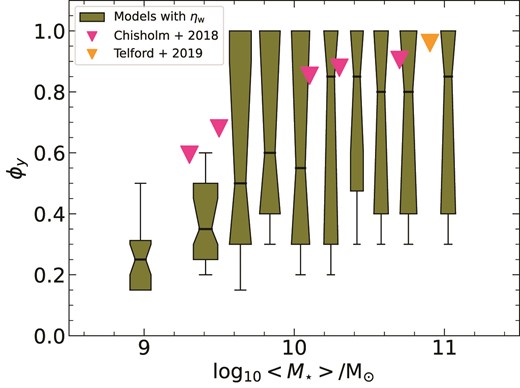
Boxplot showing the predicted scaling of ϕy that describes the preferential enrichment of galactic winds, as a function of M⋆ for local galaxies. ϕy ≈ 1 typically corresponds to wind metallicities being similar to ISM metallicities (equation 26). ϕy ≈ 0 typically corresponds to winds being very metal enriched as compared to the ISM. The predicted ϕy is based on the best match between the models with different mass-loading factors (ηw, see Section 5) and the observed MZGR from the three local IFU surveys (SAMI, MaNGA, CALIFA) as well as their overall mean. Notches denote confidence interval around the median value that is marked in solid black. Errors denote the 5th and 95th percentile range. The x-coordinate for each boxplot is the mean M⋆ across the IFU surveys. The width of the boxplot is the 1σ deviation from the mean M⋆. Pink markers denote upper limits on ϕy measured by Sharda et al. (2021b, appendix A) based on the observations of galactic wind mass-loading and metal-loading in a sample of five local galaxies by Chisholm et al. (2017), Chisholm, Tremonti & Leitherer (2018). Orange marker denotes our estimate of ϕy for M31 based on the results of Telford et al. (2019).
We also overplot ϕy for a sample of five local galaxies for which mass- and metal-loading were measured by Chisholm et al. (2017), Chisholm, Tremonti & Leitherer (2018) from Si iv and Si ii absorption features in the UV using HST/COS spectra. The corresponding ϕy values were obtained by Sharda et al. (2021b, see their appendix A).8 The predictions for ϕy are in good agreement with all the galaxies in the Chisholm, Tremonti & Leitherer sample; however, the least massive galaxy (Mrk 1486) prefers a slightly higher ϕy as compared to the predictions. Cameron et al. (2021) estimate ϕy ≈ 0.8−0.95 from measurements of ionized gas outflows for Mrk 1486. Since Chisholm, Tremonti & Leitherer and Cameron et al. only analyse the ionized phase of winds in these galaxies, it is likely that the ϕy estimated for these galaxies is an upper limit, as the hot, X-ray emitting phase can also carry a substantial amount of metals (Lopez et al. 2020, 2023). In addition to these data, we also expect ϕy ∼ 1 based on the results of Telford et al. (2019) for the local massive galaxy M31 with |$M_{\star } \approx 10^{11}\, \rm {M_{\odot }}$|. Our predicted scaling of ϕy is in qualitative agreement with the scaling of |$\mathcal {Z}_{\rm {w}}/\mathcal {Z}$| extracted by Peeples & Shankar (2011) from the MZR. It is evident that observational measurements of ϕy in diverse galaxies will be key to solving the puzzle of the role of galactic winds in driving integrated as well as spatially resolved gas-phase metal distribution in galaxies.
6 CONCLUSIONS AND FUTURE OUTLOOK
In this work, we create a model of spatially resolved gas-phase metallicities in galaxies by combining models of turbulent galactic discs in pressure and energy balance (KBFC18, Ginzburg et al. 2022) with a model for ISM metallicities (Sharda et al. 2021a). The evolution of gas-phase metallicity profiles in our model is dictated by both the large-scale properties of galaxies and properties local to the ISM. We include a comprehensive treatment of metal dynamics (advection with radial gas flows and diffusion due to turbulence powered by star formation feedback, gas transport, and cosmic accretion), and allow for preferential enrichment of galactic winds whereby wind metallicities can be higher than the ISM metallicity (see the schematic in Fig. 1). Crucially, the key parameters in our model are constrained by both local and global equilibrium, which ensures that metals are treated self-consistently with the gas and stars in galactic discs. Previous works have shown that our model also reproduces the observed relationship between |$\dot{M}_{\rm {SF}} - M_{\rm {g}}$|, ΣSFR − Σg, |$\sigma _{\rm {g}} - \dot{M}_{\rm {SF}}$|, and |$M_{\star } - \mathcal {Z}$|. Table 3 highlights the key differences in our work as compared to previous models, which are important to self-consistently model spatially resolved metallicities and metallicity gradients.
We compare the results of our model with observed metallicity gradients in local galaxies. We show that when the gas mass and velocity dispersion are calculated self-consistently, only models where turbulence is driven by a combination of feedback, transport, and accretion can reproduce the local mass-metallicity gradient relation (MZGR; see Fig. 4). Turbulence driven only by feedback or accretion produces metallicity gradients that are flatter than that observed in massive galaxies. Metal transport, if active (due to radial gas flows), plays an important role in setting metallicity gradients in low-mass galaxies.
The prescriptions of wind mass-loading we adopt from theoretical works (Hayward & Hopkins 2017; Pandya et al. 2021; Mitchell et al. 2020a) are naturally decoupled from the rest of the model. Regardless of this decoupling, we find strong evidence for the preferential metal enrichment of winds in low-mass galaxies, in line with earlier works based on modelling the MZR (Dalcanton 2007; Peeples & Shankar 2011; Sharda et al. 2021b; Tortora, Hunt & Ginolfi 2022). We also find metal loading to be more critical than mass loading in driving the MZGR. The key impact of metal-loaded winds in low-mass galaxies is to reduce the overall level of metal content in the ISM, which is necessary to reproduce the observed flatness in metallicity gradients in these galaxies without violating other gas-phase scaling relations. However, the extent of enrichment of winds in intermediate-mass and massive galaxies remains unclear because metal-loaded winds are less important (compared to feedback and accretion) for driving metallicity gradients in these galaxies (Fig. 11).
The current sample of direct measurements of wind metallicities and outflow rates is very limited and often only probes a single phase of galactic winds. Given the importance of winds in explaining both the MZR and the MZGR, it is crucial to obtain direct measurements of mass, metal, and energy loading in diverse galaxies. JWST/NIRSpec and VLT/MAVIS are expected to deliver resolved metallicity measurements for a large number of galaxies at high redshifts (Rigaut et al. 2021; Rigby et al. 2023). On the theoretical front, it is desirable to self-consistently model the CGM and the ISM so that the decoupling that currently exists between the two in chemical evolution models such as ours can be removed (Carr et al. 2022; Pandya et al. 2022). Equally important is understanding multiphase metal mixing at the CGM–ISM interface (Kim et al. 2020; Schneider et al. 2020; Vijayan, Krumholz & Wibking 2023) that occurs at pc scales not currently resolved in cosmological simulations (Gentry et al. 2019). Such a unification of ISM and CGM models can also provide a self-consistent formalism for galactic fountains that is missing from models like ours. Particularly interesting is the discovery of inverted gradients in galaxies across redshift (e.g. Cresci et al. 2010; Curti et al. 2020; Wang et al. 2019, 2022). Explaining the origin of inverted gradients within the context of gas regulator models remains a critical task for future theoretical work.
ACKNOWLEDGEMENTS
We thank the referee for their constructive report on this manuscript. We thank Aditi Vijayan and David Weinberg for going through a draft of this work and providing feedback. We also thank Simon Lilly and the AAS Journals for permitting us to adapt and modify the schematic depicting the bathtub model of chemical evolution (Fig. 1). We are grateful to Christopher Hayward, Viraj Pandya, and Joop Schaye for discussions on galactic winds. PS acknowledges support in the form of Oort Fellowship at Leiden Observatory, and the International Astronomical Union – Gruber Foundation Fellowship. OG was supported by a Milner Fellowship. MRK is supported by the Australian Research Council (ARC) Laureate Fellowship FL220100020 and Future Fellowship FT180100375. JCF is supported by the Flatiron Institute through the Simons Foundation. AD and OG were supported by the Israel Science Foundation Grant ISF 861/20. Parts of this research were supported by the ARC Centre of Excellence for All Sky Astrophysics in 3 Dimensions (ASTRO 3D), through project number CE170100013. Analysis was performed using numpy (Oliphant 2006; Harris et al. 2020) and scipy (Virtanen et al. 2020); plots were created using matplotlib (Hunter 2007), cmasher (Van der Velden 2020), and astropy (Astropy Collaboration 2013, 2018). This research has made extensive use of NASA’s Astrophysics Data System Bibliographic Services.
DATA AVAILABILITY STATEMENT
No data were generated for this work.
Footnotes
In writing equation (16), we have equated mass transport rates due to turbulent viscosity from Krumholz et al. (2018, equation 49) and Ginzburg et al. (2022, equation 39) to re-define the parameter γdiss in Ginzburg et al. (2022) as |$\gamma _{\rm {diss}} = 3/\left(2\eta \phi _Q \phi ^{3/2}_{\rm {nt}}\right)$|. Our expression differs from Ginzburg et al. (2022, equation 37) by a factor (2 + β)/2 because we also study galaxies where vϕ is not constant across the disc (i.e. galaxies with β ≠ 0). For β = 0.5, this makes a 7 per cent difference for σacc.
Leaving ηw undefined is not the same as setting it to 0 since the latter would constrain ϕy to unity as per equation (26), not permitting variations in ϕy. Since our aim in this section is to explore the full range of ϕy, we leave ηw undefined.
We use SCIPY solve_ivp to numerically integrate equation (7) from high-z to z = 0. Given the stiffness in the differential equation that arises from the different time-scales of accretion and star formation, we employ the backwards differentiation formula (BDF, Shampine & Reichelt 1997) method to search for stable solutions at each z.
The equation we solve is a sixth degree polynomial in σg, as compared to the cubic equation in Ginzburg et al. (2022) because |$\sigma _{\rm {SF}} \propto \phi ^{-3/2}_{\rm {nt}}$| (cf. equation 14) and |$\sigma _{\rm {acc}} \propto \phi ^{-3/2}_{\rm {nt}}$| (cf. equation 16). We retain the dependence of ϕnt on σg, whereas Ginzburg et al. (2022) assumed ϕnt = 1.
Note that Sharda et al. (2021a) missed a factor 1/Q in their definition of |$\mathcal {S}$| (equation 39 in their paper). This error has no impact on their results since they assumed Q = Qmin = 1.
Note that most local galaxies with |$M_{\rm {h}} \sim 10^{14}\, \rm {M_{\odot }}$| are usually ellipticals. We deliberately cover such high Mh to compare against the few massive star-forming galaxies with measured gas-phase metallicity gradients in the CALIFA survey (Sánchez et al. 2014; Sánchez-Menguiano et al. 2016).
The Chisholm, Tremonti & Leitherer (2018) sample has two additional galaxies; however, these galaxies have |$M_{\star } \lt 10^8\, \rm {M_{\odot }}$| that is beyond the mass range we consider in our models.
References
APPENDIX A: IMPACT OF VARIATIONS IN THE FRACTION OF STAR-FORMING MOLECULAR GAS
As we explain in the main text, whether massive galaxies show mass transport or not is sensitive to the star formation rate under equilibrium because transport is not needed if star formation and gas accretion are of similar strength. Thus, the existence of mass transport in the model boils down to parameters that dictate |$\dot{M}_{\rm {sf}}$|.
Variations in the fraction of star-forming molecular gas (fsf) that sets |$\dot{M}_{\rm {sf}}$| needs further exploration as previous work has shown it varies with galactocentric radius whereas we treat it as a constant in the main text. In principle, we can follow the approach used by KBFC18 to define a radially varying fsf that these authors find from the Krumholz (2013) model. However, the Krumholz (2013) model uses metallicity as an input to find fsf since the transition from atomic to molecular gas is sensitive to the ISM metallicity (Krumholz, McKee & Tumlinson 2009; Ostriker, McKee & Leroy 2010). Since metallicity is the final output of our model, it would require an iterative algorithm over several non-linear terms to model spatial variations in fsf, which is why we refrain from adopting it as our standard choice.
As a workaround, we now use the Krumholz (2013) model to find fsf where we estimate the input metallicity from the MZR. We adopt the value of fsf at r = R/2 that roughly represents the radially averaged fsf across the disc. Fig. A1 shows the resulting MZGR for the fiducial model we plot in the bottom panel of Fig. 4. We also plot the corresponding dimensionless ratios that govern the metallicity in Fig. A2. We find that transport is now active even in intermediate-mass galaxies because the average fsf is lower than the one we use in the main text, which lowers |$\dot{M}_{\rm {sf}}$|. However, the gradients produced by the model for |$M_{\star } \approx 10^{10.6}\, \rm {M_{\odot }}$| are slightly shallower than that observed, because a lower fsf decreases |$\mathcal {S}$| (cf. equation 24).

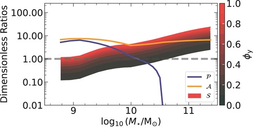
APPENDIX B: IMPACT OF UNCERTAINTIES IN THE EFFICIENCY OF ACCRETION-INDUCED TURBULENCE
The efficiency with which accreting gas can convert its kinetic into driving turbulence in the disc is described by the parameter ξa in our work. Throughout the main text, we have assumed ξa = 0.2 for all galaxies. However, as Ginzburg et al. (2022) point out, ξa is essentially a free parameter as no constraints or measurements are available for it (except from the analysis of one low-mass galaxy in the IllustrisTNG simulations by Forbes et al. 2023 that gives ξa = 0.2). It is difficult to constrain ξa because it depends on the angular momentum of the accreting gas as well as its clumpiness (Mandelker et al. 2018, 2020). In this section, we explore higher values of ξa = 0.6 and ξa = 1.0 to understand its impact on the MZGR, noting that ξa = 1 in particular is an extreme value since it implies all the kinetic energy of accreting gas goes into driving turbulent motions. We only show results for the fiducial model where σg is driven by feedback, accretion, and transport.
The top and bottom panels of Fig. B1 plot the MZGRs for the case with ξa = 0.6 and 1, respectively. The key difference between these plots and the ones we present in the main text is that the scatter due to ϕy at large M⋆ is higher. We can understand this trend with the help of σg – higher ξa leads to more turbulence due to gas accretion, and thus, higher σg. Since |$\mathcal {S} \propto \sigma ^2_{\rm {g}}$| but |$\mathcal {A} \propto \sigma ^3_{\rm {g}}$|, |$\mathcal {A}$| decreases much more as compared to |$\mathcal {S}$|, and a stronger |$\mathcal {S}$| can drive steeper, negative metallicity gradients even at high M⋆. However, it is unlikely that ξa is high in local massive galaxies, especially if a significant fraction of accreting gas is co-rotating with the disc (e.g. Danovich et al. 2015; Trapp et al. 2022).
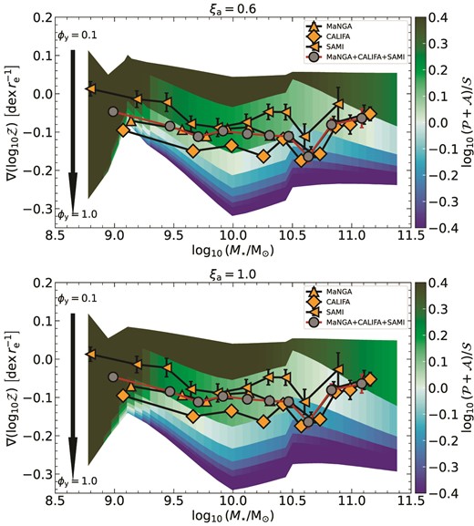
Same as the fiducial model in the bottom panel of Fig. 4 but with the ξa = 0.6 (top panel) and ξa = 1.0 (bottom panel), implying 60 per cent and 100 per cent of the kinetic energy of accreting gas goes into driving turbulent motions in the disc, respectively. The mass-loading factor (ηw) is estimated from the EAGLE cosmological simulations (Mitchell et al. 2020a).
APPENDIX C: EQUATIONS FOR CENTRAL METALLICITY
Following from Section 2.3.2, we provide here the resulting equations for the central metallicity |$\mathcal {Z}_{r_0}$|. For the case where |$\mathcal {Z}_{r_0}$| is set by the competition between source and accretion (e.g. massive galaxies),
If |$\mathcal {Z}_{r_0}$| is set by the competition between advection and diffusion (e.g. low-mass galaxies), then, in the Toomre regime of star formation,
and, in the GMC regime of star formation,
Finally, if |$\mathcal {Z}_{r_0}$| is set by the competition between source and diffusion (e.g. when transport shuts off),
APPENDIX D: SYSTEMATIC DIFFERENCES IN MZGR DUE TO METALLICITY DIAGNOSTICS
The gas-phase metallicity is typically measured using a combination of emission lines commonly found in the spectra of H ii regions. Various diagnostics of ISM metallicity exist that provide a way to convert emission line ratios to metallicity on the absolute scale (|$12+\log _{10}\rm {O/H}$|; see the reviews by Kewley, Nicholls & Sutherland 2019 and Maiolino & Mannucci 2019). These diagnostic have systematic differences that are partially responsible for the observed scatter in metallicity gradients (e.g. Poetrodjojo et al. 2021). In this section, we study the impacts of these differences on our interpretation of the MZGR. To do so, we plot the MZGR obtained from the MaNGA survey (Mingozzi et al. 2020) but for three different calibrators: PP04, based on the N ii to H α ratio, (Pettini & Pagel 2004), M08, based on O iii and O ii (Maiolino et al. 2008), and IZI (Blanc et al. 2015). Briefly, the modified version of IZI that Mingozzi et al. create uses Bayesian inference to predict the joint posterior probability distribution function (PDF) of the metallicity, ionization parameter, and extinction along the line of sight by comparing the observed emission line ratios with the Dopita et al. (2013) photoionization models.
Fig. D1 shows a comparison of the fiducial model MZGR where σg is driven by feedback, accretion, and transport with the MaNGA MZGR derived from these metallicity calibrations. The overall trend in the MZGR remains the same for all the three calibrations, as already noted by (fig. 12 of Mingozzi et al. 2020). In fact, the scatter within different surveys (MaNGA, SAMI, CALIFA) is somewhat larger than that within the same survey but different calibrators. The comparison between the model and the observed MZGR also remains unchanged. Thus, we find that systematic differences arising from different metallicity calibrations has no appreciable impact on the comparison between the model and the data.
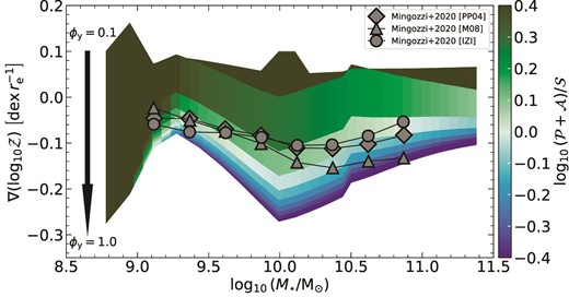
Same as the fiducial model in the bottom panel of Fig. 4 but the overplotted data is from the MaNGA survey (Mingozzi et al. 2020) using three different metallicity calibrations: PP04 (Pettini & Pagel 2004), M08 (Maiolino et al. 2008), and IZI (Blanc et al. 2015). The mass-loading factor (ηw) is estimated from the EAGLE cosmological simulations (Mitchell et al. 2020a).
