


ABSTRACT
We report a detailed multi-wavelength study of the supernova remnant G296.5+10.0 using archival data from XMM–Newton and Fermi-LAT complemented with ATCA observations. In the X-ray band, we performed an adaptive smoothing on the double background subtracted images to construct an X-ray mosaic map with six individual observations. Below 2.0 keV, G296.5+10.0 is asymmetrical, with the south-east side of the radio shell brighter than the south-west one. The spatially resolved X-ray spectral study confirms the thermal origin of the plasma, with enhanced metal abundances, probably arising from ejecta material according to the H i and infrared (|$140~{\mu \rm m}$|) distributions. In the γ-ray band, we analysed 14 years of accumulated Fermi observations below 500 GeV via different fitting processes. To discuss the origin of the γ-ray emission, we compare the GeV results with H i structures probably associated with the SNR and with the radio spectral indices found at various positions towards the radio shell. Moreover, we identified diverse sources candidates to contribute γ-ray emissions observed. Also, we calculated the lepto-hadronic spectral energy distribution of the remnant for synchrotron, inverse Compton, Bremsstrahlung, and proton–proton processes. The emission at low energies can be explained by electron-synchrotron radiation, with a weak magnetic field of |$B=25\, {\rm \mu G}$|, while the γ-ray data can be explained by hadronic interactions. Employing the reddening-distance method, we computed a distance of 1.4 kpc for the SNR, implying an age of 14 000 yr.
1 INTRODUCTION
Supernova remnants (SNRs) are classified, according to the morphological features observed in the radio and X-ray bands, as shell-like, plerionic, and composite or mixed-morphology (MM). Their appearance is determined by the mass loss history of the exploding star, the supernova (SN) event itself, the possible remaining central compact object (CCO), the ambient magnetic field and the surrounding interstellar medium (ISM) where the remnant evolves. Many shell-type SNRs, far from being circular, depict a barrel-like shape, giving rise to a new subgroup in this classification (Kesteven 1987; Kesteven & Caswell 1987). SNRs belonging to this subclass, also called bipolar or bilateral (Fulbright & Reynolds 1990), are characterized by two opposing bright limbs allocated on either side about an axis of cylindrical symmetry, with low or null emission between them.
Gaensler (1998) summarizes several possible reasons proposed to explain the appearance of bilateral SNRs, differentiating between intrinsic (e.g. toroidal distribution of ejecta, the effect of a high-velocity progenitor, the distribution of mass loss and magnetic field in the circumstellar medium produced by the progenitor, the influence of outflows from a CCO) and extrinsic reasons (e.g. expansion of the remnant inside a tube-like cavity, or the geometry of the ambient magnetic field). The Galactic SNR G296.5+10.0 constitutes a prototypical case of this peculiar subclass, exhibiting a bilateral morphology with a striking axial symmetry in the radio band.
In radio, G296.5+10.0 has a 90 × 65 arcmin-size with its symmetry axis almost perpendicular to the Galactic plane. This source was first classified as a SNR based on the spectral index α = 0.5 (defined as Sν ∝ ν−α) obtained from different observations at 0.2, 0.6, and 1.4 GHz (Whiteoak & Gardner 1968). The authors also reported that the radio emission is distributed along two ridges, as was later confirmed with observations at 5 GHz (Milne 1970). Roger et al. (1988) carried out a high-resolution radio observation with the Molonglo Observatory Synthesis Telescope (MOST) at 843 MHz, revealing a fine structure in the form of filaments aligned tangentially to the SNR shell, which are interpreted as multiple thin sheets of emission or crushed clouds viewed edge-on. Harvey-Smith et al. (2010) studied the Faraday rotation of G296.5+10.0 using spectropolarimetric images at 1.4 GHz obtained with the Australia Telescope Compact Array (ATCA). They found that the source displays a highly ordered rotation measure (RM) structure, with positive and negative values on the eastern and western sides of the shell, respectively, which they explained through an azimuthal magnetic field produced by the progenitor stellar wind (but see Mabey et al. 2020, who dispute this interpretation and prefer a uniform magnetic field). Giacani et al. (2000) presented H i observations in a 3|${_{.}^{\circ}}$|5 × 3|${_{.}^{\circ}}$|5 fields around G296.5+10.0 using ATCA and found that some H i structures between −17.5 and |$-15.5\,{\rm km}\, {\rm s}^{-1}$| could be apparently linked to the SNR. This result locates the SNR at a distance of ∼2.1 kpc based on Galactic rotation models (Giacani et al. 2000).
The first X-rays observations of G296.5+10.0 were reported by Tuohy et al. (1979) using the HEAO-1 A2 experiment. They found an X-ray peak correlated to the south-east part of the radio shell. In the following years, observations from the Einstein Observatory (Helfand & Becker 1984; Matsui, Long & Tuohy 1988) showed the detailed distribution of the X-ray emission over the eastern part, with a weak component at the south-west of the SNR. No significant X-rays were found in the north-west. An X-rays analysis on the eastern side of G296.5+10.0 based on data from the EXOSAT Position Sensitive Detector (PSD; Kellett et al. 1987) revealed a thermal origin for the plasma between 0.1–1.2 keV. Also, the X-ray map showed a localized region of low X-ray surface brightness, or hole, that lies between two radio peaks aligned N–S at the south-east of the shell and is bordered all around by a ridge of enhanced X-rays emission. Based on these results, Kellett et al. (1987) proposed that the X-ray emission could be associated with the cloud evaporation process.
The X-ray image obtained by Helfand & Becker (1984) also revealed the presence of the CCO 1E 1207.4–5209 in proximity to the centre of the SNR, which has no counterpart in the radio band. Kellett et al. (1987) suggested that this X-ray object (dubbed EXO120723-5209.8 by the authors) could be the neutron star related to G296.5+10.0. Following this scenario, Zavlin, Pavlov & Trumper (1998) found that 1E 1207.4–5209 could be placed at a distance in the range 1.6-3.3 kpc, in very good agreement with the kinematic distance estimated in Giacani et al. (2000). A small H i depression strikingly coincident in position with the CCO between the velocities −16.1 and |$-15.8\,{\rm km}\, {\rm s}^{-1}$| (Giacani et al. 2000) renders further support to a possible neutron star-SNR association. Zavlin et al. (2000) found 1E 1207.4–5209 to be the first CCO with pulsating X-rays emission. A revised analysis of the timing data (Gotthelf & Halpern 2007) revealed a noticeable stable rotation period (in spite of a few glitches detected recently; Gotthelf & Halpern 2020), implying a lack of magnetic activity. A proper motion measurement (Halpern & Gotthelf 2015) demonstrates that the pulsar has scarcely moved during the lifetime of G296.5+10.0, hence its off-centred position from the geometrical centre of the radio shell could imply either an asymmetrical SN explosion or an asymmetrical evolution of the SNR, or both.
At γ-ray energies, G296.5+10.0 was first studied by Araya (2013) using fifty-two months of accumulated Fermi-LAT observations (Pass 7 data). The cited work reported the detection of a (seemingly) extended γ-ray source, although the fitted extended disc model did not sufficiently improve the point-source hypothesis to claim a clear detection of extension. The author concluded that both leptonic and hadronic mechanisms could account for its high-energy emission. G296.5+10.0 was later included in the first Fermi-LAT SNR catalogue (Acero et al. 2016) with significant evidence of extension and a radius of 0|${_{.}^{\circ}}$|76 ± 0|${_{.}^{\circ}}$|08. The Fermi High-Latitude Extended Sources Catalog (Ackermann et al. 2018) also listed G296.5+10.0 (as FHES J1208.7-5229), in this case with 0|${_{.}^{\circ}}$|7 radius of extension at very high significance. More recently, the re-analysis of LAT γ-ray data from the source performed by Zeng et al. (2021) favoured a hadronic scenario for the origin of its γ-ray emission.
It is clear that several aspects related to G296.5+10.0 still need to be explained. We expect that a detailed spectroscopical analysis of the X-rays emission will provide useful clues to unveil the origin of different peculiar features, like the eastern ridge and hole (Bingham et al. 2004). With this goal in mind, in this paper we report a high-energy study of the SNR G296.5+10.0 processing archival data of the XMM–Newton telescope and, in addition, of the Fermi-LAT at energies between 100 MeV and 500 GeV. We complement this study with H i and radio continuum data. The structure of the paper is as follows: in Section 2, we describe the XMM–Newton and Fermi-LAT observations and the data reduction process, including the radio data. X-ray/γ-ray analysis and results are shown in Section 3. In Section 4, we discuss the implications of our results including an analysis of the spectral energy distribution of the remnant, from the radio to the γ-ray data. Finally, we summarize our main conclusions in Section 5.
2 OBSERVATIONS AND DATA REDUCTION
2.1 XMM–Newton observations
The full extension of G296.5+10.0 has been observed six times with the European Photon Imaging Camera (EPIC) of the XMM–Newton satellite. This camera consists of three detectors: two MOS cameras, namely MOS1 and MOS2 (Turner et al. 2001), and a PN camera (Strüder et al. 2001), which operate in the 0.3–10 keV energy range. The five sets towards the SNR G296.5+10.0 were made with a thin filter in Full Frame Mode, and they are available in the data base of XMM–Newton telescope. The observation with ID 0862990201 was made in the direction of source 1E 1207.4–5209. From this last data set, the EPIC-MOS cameras have a medium filter in Full Frame Mode, while the EPIC-PN has a thin filter in Small window.
The EPIC MOS background components are mainly electronic noise, fluorescence emission lines (instrumental background, not vignetted), X-ray Galactic emission (astrophysical background, vignetted), and soft magnetospheric protons focused by the optics (Lumb et al. 2002; Marty et al. 2003). Since G296.5+10.0 is an extended source that fills most of the field of view, it is not possible to estimate the local astrophysical background from the same data. Instead of a local background, we used the MOS1, MOS2, and PN sets of blank sky (BS) files (Carter & Read 2007) pointed towards a Galactic longitude of 296|${_{.}^{\circ}}$|5 and a Galactic latitude 10|${_{.}^{\circ}}$|0 with a radius of 4000 arcsec. The BS sets were scaled by the relative exposure time and then reprojected into the sky altitude of G296.5+10.0 pointings with the script skycast (see Section 5 in Carter & Read 2007). Furthermore, we downloaded the Filter Wheel Closed (FWC) files1 to correct the five observations by the instrumental background response of the XMM–Newton satellite.
For the data reduction of each observation, we used the heasoft version 6.26.1 and the Science Analysis System (SAS) version 18.0.0. We first generated calibrated events files with the emproc and epproc tasks. In order to avoid strong background flares, we extracted light curves of the full field of view for each camera above 10 keV, excluding intervals 3σ above the mean count rate to produce good-time interval (GTI) files. Also, we filtered these event files using the evselect task to retain only photons likely to be X-ray events. In this last procedure, we selected events with FLAG = 0, PATTERN 0 to 4 and energies 0.2 to 15 keV for the PN, and PATTERN 0 to 12 and energies 0.2 to 12 keV for MOS1/2 instruments. We found background contamination in the PN data in Obs. ID-0762090301 and ID-0762090501; hence, those PN events were discarded from the following X-ray study. For Obs. ID-0781720101 and ID-0762090201, the CCD 3 and CCD 6, respectively, were lacking in the MOS1 camera and the spectra for some of the regions could not be taken (see Section 3.2). In Table 1, we report a summary of the observations: Obs-Id, date, pointing centre coordinates, and exposure time before and after flare screening.
XMM–Newton observations of G296.5+10.0.
| ID Obs | Date | R.A. | Dec. | Exposures | GTI |
|---|---|---|---|---|---|
| (UT) | (J2000) | (J2000) | (ks) | (ks) | |
| 0781720101 | 2016-06-27 | 12 12 27.45 | −52 17 19.9 | 27.4-27.6/22.6 | 26.2-25.5/20.1 |
| 0762090201 | 2016-02-14 | 12 11 33.05 | −52 41 05.7 | 26.3-26.4/24.6 | 22.9-24.5/21.3 |
| 0762090301 | 2016-01-15 | 12 10 20.39 | −52 56 20.6 | 26.7-26.3/24.1 | 24.6-23.5/4.3 |
| 0762090401 | 2016-02-16 | 12 08 18.28 | −52 55 50.5 | 31.3-31.2/26.2 | 25.2-24.3/20.1 |
| 0762090501 | 2016-02-16 | 12 07 01.75 | −52 39 11.1 | 27.4-27.2/22.3 | 20.3-21.5/5.2 |
| 0862990201 | 2020-06-22 | 12 10 0.17 | −52 26 31.9 | 33.1-33.2/23.2 | 29.8-28.5/16.3 |
Note. Units of right ascension are h, m, s, and units of declination are °, ′, ″. The Exposure times and GTI are given for the MOS1-MOS2/PN cameras.
2.2 Fermi-LAT data selection and analysis tools
To study the high-energy γ-ray emission towards the SNR G296.5+10.0, we analysed the Fermi-LAT data at energies from 100 MeV to 500 GeV. The archival LAT data were from 2008, August 4th to 2022, September 29th, or from 239557417 to 686106544 seconds in Fermi Mission Elapsed Time (MET). We establish as a region of interest (ROI) a 15° radius around the reference position (R.A., Dec.) = (182|${_{.}^{\circ}}$|4, −52|${_{.}^{\circ}}$|4), the central coordinate of G296.5+10.0 according to Green (2019). We selected and processed the dubbed source class events to include only those that are γ-rays at high probability, setting a maximum zenith angle of 90° to avoid events closer to the limb of the Earth. The data reduction was performed using the fermipy python package (version 1.0.1, Wood et al. 2017) and the Fermi Science Tools2 version 2.0.8.
The sources represented in the ROI model are listed in the third data release of the fourth Fermi-LAT source catalogue (4FGL-DR3, last updated on 2022, May 11th; Abdollahi et al. 2022). The data were fitted with a model that includes all 4FGL-DR3 sources in a radius of 20° around the centre of the ROI. In addition, we characterized the diffuse background emission with the Galactic and isotropic diffuse emission models3 with the version gll_iem_v07 and iso_P8R3_SOURCE_V2_v1. The data were binned into eight energy bins per decade and spatial bins with 0|${_{.}^{\circ}}$|1 of size. Then, we applied an energy dispersion correction except in the isotropic diffuse emission.
We approximated the sources detection significance as the square root of the test statistic (TS), defined as |$\rm {TS} = 2\log (\rm {L/L_{0}})$|, where L is the maximum value of the likelihood function over the ROI (including the source in the model) and L0 is the same but only accounting for background (Mattox et al. 1996). The free parameters of the model are the normalization of all sources with TS >10 and all spectral parameters for sources in a 5° radius around the centre of the ROI, except the reference energy. The spectral models characterizing the isotropic and Galactic background emission, which are provided by the Fermi Science Tools, are multiplied by a constant and power-law component, respectively. The normalization parameter of both components, and the slope (tilt) in the case of the power-law one for the Galactic diffuse emission model, are also set free.
We fitted a power law (dN/dE = N0 × (E/E0)−Γ) and an exponentially cut-off power-law (|${\rm d}N/{\rm d}E = N_{0} \times (E/E_0)^{-\Gamma}\times {\rm e}^{-E/E_{\rm cutoff}}$|) function to the LAT spectral energy distribution (SED) of SNR G296.5+10.0 (4FGL J1208.5-5243e) using the fermipy sed method for twelve energy bins ranging from 100 MeV to 300 GeV. Also, we probed the extension of the source with the extension method, based on the calculation of a likelihood ratio test with respect to the point-source hypothesis. For the latter, we used both the radial Gaussian and the disc-shaped spatial models characterized by intrinsic sizes of σ = r68/1.51 and R = r68/0.82 (where r68 is the 68 per cent containment radius, CR; Lande et al. 2012), respectively. Then, we computed the position for the peak emission of the source with the localize method, surveying the likelihood function in a local region with a size of 0|${_{.}^{\circ}}$|5 around the reference position.
To evaluate the significance of the emission towards different directions, we mapped the TS throughout the ROI with the tsmap method of fermipy. The latter method moves a putative point source (we used an index 2 power-law spectrum) throughout a grid of locations in the sky and maximizes the log-likelihood function at each grid point. We applied this method for ten different energy thresholds from 100 MeV to 20 GeV to map the emission of the source at different energy ranges. Moreover, we repeated the analysis summarized above for six differential energy bins with break-points at energies of 0.1, 0.8, 3, 10, 20, 50, and 500 GeV to search for hints of energy-dependent morphology.
We analysed the LAT data downloaded above 3 GeV of threshold energy to examine the source’s morphology more in-depth. The improvement of the LAT PSF, which is smaller than ∼0.25 (68 per cent CR) above a few GeV of energy compared to ∼0|${_{.}^{\circ}}$|85 at 1 GeV, facilitates the latter analysis. Then, we followed two approaches. First, we fitted to the LAT data different models for the γ-ray source involving either one or two components. Namely, we used the (normalized) radio emission from the SNR shell as a spatial template for the source to be compared with the (simple) radial Gaussian and disc models. Also, we considered modelling the source with the cited shell spatial template plus an inner (power-law) point source at two different positions: (1) one close to both the X-ray pulsar dubbed 1E 1207.4–5209 and the prominent H i cloud lying near the brightest filaments at the east radio limb of the remnant (R.A. = 182|${_{.}^{\circ}}$|6 and Dec = −52|${_{.}^{\circ}}$|7); (2) the other near the noticeable radio sources located towards R.A. = 182|${_{.}^{\circ}}$|0 and Dec = −52|${_{.}^{\circ}}$|2.
For the second approach, we applied a grid to a 3|${_{.}^{\circ}}$|1 × 3|${_{.}^{\circ}}$|1 region containing the source, with a spacing comparable in size to the LAT acceptance-weighted PSF (68 per cent CR) at an energy of a few GeV (i.e. 0|${_{.}^{\circ}}$|24). The next step was to replace the (4FGL-DR3) catalogued model for the SNR G296.5+10.0 with a set of putative power-law point sources, adding one by one at the grid cells, where significant emission is observed according to the TS maps described above. Among these sources, only those with |$\sqrt{\rm TS} \gtrsim 16$| and positionally coincident with the remnant (or within the shell) are retained in the model. After adding each source to the ROI model, all spectral sources (power law) are fitted jointly. Also, we re-fitted their positions in each iteration. Lastly, we checked whether the log-likelihood of the (global) model fitted to the data is equal or larger than the value obtained considering only one extended source. Note that the difference of degrees of freedom among the hypotheses is Δk = 4 × N − 5, where N is the number of putative point sources, compared to a unique extended source model. This fitting process allows us to survey the flux and spectral index in different directions along the extended source. In this energy regime, the LAT PSF is smaller, by more than a factor 3 indeed, than the (68 per cent CR) γ-ray radius previously fitted to the source (∼0|${_{.}^{\circ}}$|72) when a unique extended source is considered.
To conclude, we tested the consistency of our results by studying the systematic uncertainties in the spectrum of the source, mainly due to the LAT effective area and the Galactic diffuse emission model. We estimated the former systematic uncertainties with the dubbed bracketing effective area method4 and those due to the diffuse Galactic model by artificially changing its normalization by ±6 per cent compared to the best-fitted value (Abdo et al. 2010; Ajello et al. 2012).
2.3 H i and radio continuum data reduction
To analyse the H i distribution towards G296.5+10.0, we reprocessed archival observations carried out during 1998 with the Australia Telescope Compact Array (ATCA) under project code C738 (Giacani et al. 2000). To cover a wide area around the large extension spanned by G296.5+10.0, the mosaicing technique was applied with 109 pointings following an hexagonal grid arranged so as to fulfill the Nyquist sampling criterion. The ATCA was used in the non-standard |$210~\rm m$| configuration, with baselines varying from 30.6 to 214.2 m considering the five movable antennae (the 6th, fixed antenna was excluded). A correlator of 1024 channels, each with a 4 kHz width, was used. At a central frequency of 1420 MHz, the channel width is equivalent to |$0.825\,{\rm m}\, {\rm s}^{-1}$|. The flux and phase calibrators were PKS 1934–638 and PKS 1215–457, respectively. Standard data reduction was carried out using the software reduction package miriad (Sault, Teuben & Wright 1995). The continuum emission was subtracted in the u, v-plane after selecting two separate sets of line-free channels. All pointings were deconvolved jointly, but in contrast with Giacani et al. (2000), we employed the task mossdi instead of mosmem to allow for negative clean components. Also, to complete the visibility coverage with the shortest spatial frequencies, we added observations performed with the Parkes 64-m radio telescope (now called Murriyang) obtained from the public H i Galactic All Sky Survey (GASS; McClure-Griffiths et al. 2009; Kalberla et al. 2010). In the |$210~\rm m$| configuration, the ATCA has four antenna pairs with baselines shorter than 64 m, providing an excellent overlap with the single dish data in the u,v-plane. In this sense, the H i data set used here is an improvement with respect to Giacani et al. (2000), who obtained the single dish data from a 30 m antenna, hence with no overlap with the interferometric observations. A data cube was created with 1000 channels from −345.0 to |$417.2\,{\rm m}\, {\rm s}^{-1}$| and a synthesized beam of 273|${_{.}^{\prime\prime}}$|9 × 179|${_{.}^{\prime\prime}}$|7, with position angle 0|${_{.}^{\circ}}$|3. An rms of ∼0.6 K was attained in the line-free channels.
We also calibrated the radio continuum observations that were simultaneously observed with the H i line data. The observations, centred at 1384 MHz, were obtained through a 128 MHz bandwidth correlator split in 324-MHz channels. A joint calibration was performed with the miriad task pmosmem. The continuum image was constructed with a circular beam of 210 arcsec to match the resolution of the 4.85 GHz continuum image from the Parkes-MIT-NRAO (PMN) survey (Condon, Griffith & Wright 1993). Finally, this image was merged with archival single dish observations performed with the Parkes 64-m antenna obtained from the Continuum HI Parkes All Sky Survey (CHIPASS; Calabretta, Staveley-Smith & Barnes 2014). The resulting rms is |${\le}2.5\,{\rm mJy\, beam}^{-1}$|. This image will be used solely to compute spectral indices as explained later in Section 4.4. Throughout the rest of the paper, we will make use of the higher resolution image at 843 MHz downloaded from the Molonglo Galactic Plane Survey (MGPS-1; Green et al. 1999).
3 RESULTS
3.1 X-ray images
In order to analyse in detail the X-ray morphology of G296.5+10.0 and to study the spatial correlation with the radio and γ-ray emissions, we performed a point-source detection by running the edetect_chain script. This procedure allowed us to focus on the diffuse emission, removing the events in circular regions of 10 arcsec from the filtered event files that we selected with FLAG = 0 and single and double PATTERNs (see Section 2.1). Then, we created a mosaic image of the entire SNR by combining the data from the six different pointings of the MOS1 and MOS2 cameras, using the SAS tasks merge and evselect. We applied a double background subtraction as described in Miceli et al. (2017) by using BS and FWC data (see Section 2.1) to obtain the counts mosaic subtracted image from each observation. The mosaic was built in counts, and adaptive smoothing was applied such that the signal-to-noise ratio was at least 10.
Fig. 1 displays a false-colour image of the extended X-ray emission towards the SNR G296.5+10.0 between 0.4–2.0 keV, showing the spatial correlation with the radio image at 843 MHz, indicated in white contours. This figure shows the emission of the plasma in the different energy ranges: the soft band (0.4–0.6 keV) is plotted in red, the medium band (0.6–0.9 keV) in green, and the hard band (0.9–2.0 keV) in blue. The X-ray emission of the remnant is dominated by the contribution of the soft and medium bands, while the hard band emission appears only on the south-eastern limb of the radio shell, coincident in position with the brightest regions at the internal edge near the centre.
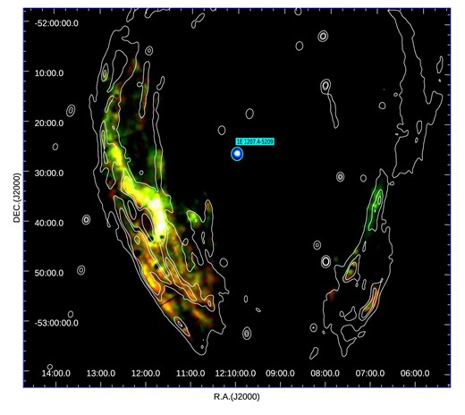
X-ray false-colour image linear-scaled of the SNR G296.5+10.0 in the three X-ray energy bands: soft (0.4–0.6 keV) in red, medium (0.6–0.9 keV) in green, and hard (0.9–2.0 keV) in blue. The radio continuum emission at 843 GHz is indicated in white contours at 0.041, 0.18, and |$0.24\,{\rm mJy\, beam}^{-1}$|. The cyan circle indicates the position of the neutron star 1E 1207.4–5209, which is believed to be associated with the SNR. The North is up and the East is to the left.
The X-ray mosaic map with the six pointing covers ∼70 per cent of the radio emission, since there are no XMM–Newton data from the northern regions of the radio limbs. Also, the remnant is undetected above 2.0 keV in XMM–Newton observations.
3.2 X-ray spectral analysis
In order to study the physical conditions of the plasma, we performed a spatially resolved spectral analysis of the SNR using the six XMM–Newton observations. Based on the morphology observed in the X-ray images, we produced spectra in twelve different regions. These regions were chosen to be large enough to obtain good photon statistics and small enough to admit the comparison of their plasma conditions. Spectra were obtained using the evselect SAS task with the appropriate parameters for EPIC MOS 1/2 cameras, and the background was subtracted using the XMM–Newton Blank Sky files (Carter & Read 2007) for the same regions. Since the X-ray emission occupies most of the field of view, we applied the SAS evigweight task to correct the event lists for vignetting effects. The X-ray spectrum of the SNR presents a relatively low signal below 0.4 keV, therefore we restrict the analysis to the range of 0.4–2.0 keV. Fig. 2 shows a background subtracted image of the X-ray emission and the twelve regions indicated in green colour. The response and ancillary matrices were obtained with the rmfgen and arfgen tasks and the spectra were grouped with a minimum of 16 counts per bin. Error bars were quoted at 90 per cent and a χ2 statistic was used. The spectral analysis was performed using the X-Ray Spectral fitting package (XSPEC; Arnaud 1996) and the line emission information was obtained from the AtomDB5 data base (version 3.0.9).
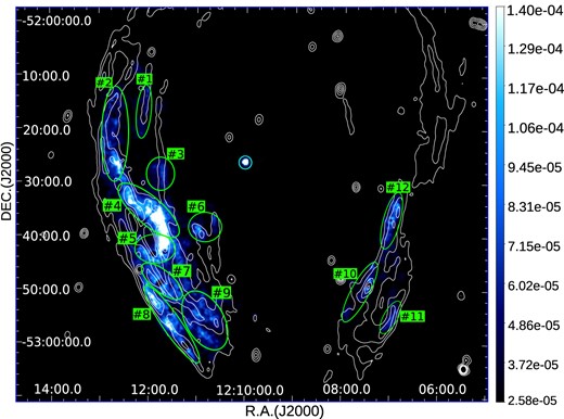
Mosaic double background subtracted image linear-scaled of the six observations in the X-ray band towards the SNR G296.5+10.0. The twelve regions selected for the spectral analysis are indicated in green (see Section 3.2). The cyan circle indicates the position of the neutron star 1E 1207.4–5209. The white contours at 0.03, 0.16, 0.24, and 0.32|$~{\rm mJy\, beam}^{-1}$| represent the radio emission. The North is up and East is to the left.
Fig. 3 shows the X-ray spectra of the twelve regions selected on the SNR G296.5+10.0. From each spectra, we noticed the presence of several strong emission lines of O vii (0.57 keV), O viii (0.65 keV), Fe xviii (0.77 keV), Ne ix (0.92 keV), Mg xi (1.33 keV), and Fe xx (1.36 keV). To constrain the astrophysical conditions of the thermal emission, we adopted a collisional ionization equilibrium (CIE) model and fitted each region with a single VAPEC model (Smith & Hughes 2010), thus confirming the thermal nature of the emitting plasma. The foreground NH was modelled using the Tuebingen-Boulder absorption model (TBABS; Wilms, Allen & McCray 2000). We left free the abundances of O, Ne, Mg, and Fe, all other element abundances were fixed at their solar values. The X-ray parameters of the best fit to the diffuse emission spectra for the different regions are presented in Table 2. In general, the fitted electron temperature of the plasma is about 0.15 keV, which is in good agreement with the 1.35–1.77 × 10⁶ K temperatures (0.11–0.15 keV) found in Kellett et al. (1987). According to the fits, the values of NH range from 0.74 × 10²¹ to 0.85 × 1021 cm−2, while in in Kellett et al. (1987) the average column density is ∼1.84 × 1021 cm−2.

Spatially resolved X-ray spectra of the twelve regions selected on the SNR G296.5+10.0 (see Fig. 2). In each plot, the levels of the vertical axis are counts |${\rm cm}^{-2}\, {\rm s}^{-1}\, {\rm keV}^{-1}$| for the top panel and (data-model)/error for the bottom panel. The X-ray emission corresponding to the EPIC PN, MOS1, and MOS2 cameras are in green, red, and black, respectively. For region #8, we combined the X-ray spectra from ID Obs 0762090201 and 0762090301. In this last plot, we indicated the PN camera in green for both observations, MOS1 in red and cyan and MOS2 in black and blue.
Spectral parameters of the X-ray emission of G296.5+10.0.
| Parameters | #1 | #2 | #3 | #4 | #5 | #6 | #7 | #8 | #9 | #10 | #11 | #12 |
|---|---|---|---|---|---|---|---|---|---|---|---|---|
| NH (1021) | 0.83 ± 0.01 | 0.84 ± 0.01 | 0.81 ± 0.01 | 0.82 ± 0.01 | 0.85 ± 0.01 | 0.74 ± 0.01 | 0.81 ± 0.01 | 0.79 ± 0.02 | 0.83 ± 0.02 | 0.82 ± 0.01 | 0.82 ± 0.01 | 0.77 ± 0.02 |
| kT | 0.14 ± 0.01 | 0.16 ± 0.01 | 0.16 ± 0.01 | 0.17 ± 0.01 | 0.15 ± 0.01 | 0.16 ± 0.02 | 0.15 ± 0.01 | 0.14 ± 0.01 | 0.14 ± 0.02 | 0.14 ± 0.01 | 0.14 ± 0.01 | 0.14 ± 0.02 |
| O | 0.4 ± 0.2 | 0.9 ± 0.1 | 0.7 ± 0.1 | 0.6 ± 0.2 | 0.7 ± 0.1 | 0.5 ± 0.1 | 0.4 ± 0.1 | 0.2 ± 0.1 | 0.6 ± 0.1 | 0.6 ± 0.1 | 0.7 ± 0.1 | 0.7 ± 0.1 |
| Ne | 1.2 ± 0.1 | 2.2 ± 0.1 | 1.6 ± 0.3 | 1.7 ± 0.1 | 1.9 ± 0.1 | 0.7 ± 0.1 | 1.2 ± 0.1 | 0.5 ± 0.1 | 1.8 ± 0.2 | 1.5 ± 0.2 | 1.7 ± 0.3 | 2.3 ± 0.2 |
| Mg | 1.7 ± 0.7 | 1.0 | 1.0 | 3.3 ± 0.5 | 3.8 ± 0.9 | 1.0 | 1.0 | 1.0 | 1.0 | 1.0 | 1.0 | 1.0 |
| Fe | 1.5 ± 0.2 | 3.1 ± 0.2 | 1.9 ± 0.4 | 2.6 ± 0.2 | 2.9 ± 0.5 | 1.6 ± 0.4 | 1.7 ± 0.3 | 1.9 ± 0.8 | 1.5 ± 0.9 | 1.3 ± 0.4 | 2.2 ± 0.8 | 3.9 ± 0.9 |
| Norm(10−3) | 8.3 ± 0.2 | 8.6 ± 0.3 | 3.9 ± 0.2 | 8.1 ± 0.2 | 9.8 ± 0.1 | 3.5 ± 0.1 | 8.0 ± 0.2 | 7.5 ± 0.2 | 9.2 ± 0.3 | 8.1 ± 0.2 | 4.4 ± 0.2 | 8.9 ± 0.2 |
| Flux0 (10−13) | 39.1 ± 0.4 | 74.7 ± 0.8 | 36.9 ± 0.7 | 108.7 ± 0.6 | 88.5 ± 0.7 | 23.1 ± 0.4 | 46.3 ± 0.4 | 35.6 ± 0.4 | 62.2 ± 1.1 | 51.8 ± 0.8 | 27.2 ± 0.8 | 69.3 ± 1.2 |
| |$\chi _\nu ^{2}$|/d.o.f. | 1.5/508 | 1.6/524 | 1.4/499 | 1.6/511 | 1.5/513 | 1.3/490 | 1.6/498 | 1.3/575 | 1.6/405 | 1.4/520 | 1.1/399 | 1.4/206 |
| EM (1056) | 1.94 | 2.02 | 0.91 | 1.90 | 2.29 | 0.82 | 1.87 | 1.75 | 2.15 | 1.89 | 1.03 | 2.08 |
| ne | 0.19 | 0.12 | 0.14 | 0.14 | 0.17 | 0.11 | 0.19 | 0.19 | 0.15 | 0.14 | 0.12 | 0.15 |
Note. The twelve spectral regions were fitted with a VAPEC model. NH was computed from TBABS XSPEC model in units of cm−2. kT is the electron temperature in units of keV. Norm is the normalization of the fitted models defined as |$10^{-14}/4\pi \, d^2 \times \int n_{\rm H} n_{\rm e}\, {\rm d}V$|, where d is the distance in cm, nH is the hydrogen density in units of cm−3, ne is the electron density in cm−3, and V is the emitting volume in cm3. Flux0 refers to the intrinsic flux in units of |${\rm erg}\, {\rm s}^{-1}\, {\rm cm}^{-2}$|. EM is the emission measure of the X-ray plasma in units of cm−3, defined as |$\int n_{\rm H} n_{\rm e}\, {\rm d}V$|.
We detected ionization lines with different abundances depending on each region. The relative abundances of O are subsolar or close to solar abundances in almost every region. The fitted abundances for Ne are significant in regions #2 (∼2.2), #4 (∼1.7), #5 (∼1.9), #9 (∼1.8), and #12 (∼2.3). The abundances of Mg are only high in regions #4 (∼3.3) and #5 (∼3.8). Regions #2, #4, #5, #11, and #12 also present high abundances of Fe, of about 3.1, 2.6, 2.9, 2.2, and 3.9, respectively. We also found that the unabsorbed X-ray flux (Flux0) is larger in regions where the metal abundances are significant, i.e. regions #2, #4, and #5. The Flux0 ranges from 23.1 to |$108.7 \times 10^{-13}\,{\rm erg}\, {\rm s}^{-1}\, {\rm cm}^{-2}$| (see Table 2), the highest value corresponding to region #4. Considering both the enhanced abundances and the variation of Flux0 among the different regions, these results could be indicating that the X-ray emitting plasma is dominated by the ejecta with a mix of shocked clouds from the surrounding ISM.
3.3 γ-ray analysis
The best-fitting model located the peak of the extended γ-ray emission at RA = 182|${_{.}^{\circ}}$|167 ± 0|${_{.}^{\circ}}$|045, Dec. =−52|${_{.}^{\circ}}$|507 ± 0|${_{.}^{\circ}}$|051 (only statistical errors) with a large detection significance of |$\sqrt{\rm TS} \approx 17\sigma$|. This position is thus well centred within the radio shell and in good agreement with Araya (2013) and Zeng et al. (2021) taking into account statistical and systematic errors.
The parameters of the best-fit power-law spectral model took the values |$N_{0} = (7.27 \pm 0.52_{\rm stat} \pm 0.28_{\rm syst}) \times 10^{-14}\, {\rm cm}^{-2}\, {\rm s}^{-1}\, {\rm MeV}^{-1}$| referenced at E0 = 4056.5 MeV, and Γ = 1.93 ± 0.05stat ± 0.02syst, which implies |$(5.1 \pm 0.7) \times 10^{-9}\, {\rm ph}\, {\rm cm}^{-2}\, {\rm s}^{-1}$| of integrated flux from 200 MeV to 100 GeV. For simplicity, the systematical errors due to the LAT effective area and the Galactic diffuse emission were added in quadrature. The spectrum of the γ-ray source does not exhibit any apparent curvature from 500 MeV to 200 GeV. The exponential power-law cut-off fit of the spectrum placed the cut-off at an energy of Ecutoff = 284 ± 106stat ± 30syst GeV, which does not improve the simple power-law fit according to the Akaike information criterion (AIC, with AICECPL − AICPL ≈ 2.7; Akaike 1973, 1974). From comparing the power-law modelling with the exponential cut-off power-law one at different (fixed) cut-off energies through the likelihood ratio test, we conclude that if the LAT SED presents an exponential cut-off, it must be located at an energy greater than ∼80 GeV at a 95 per cent confidence level (CL).
The γ-ray emission is significantly extended above 500 MeV, with |$\sqrt{\rm TS} \sim 15.5\sigma$| compared to the point source hypothesis, r68 = 0|${_{.}^{\circ}}$|731 + 0|${_{.}^{\circ}}$|049 − 0|${_{.}^{\circ}}$|046 (σ = 0|${_{.}^{\circ}}$|484 + 0|${_{.}^{\circ}}$|032 − 0|${_{.}^{\circ}}$|031) for the Gaussian spatial model, and r68 = 0|${_{.}^{\circ}}$|714 + 0|${_{.}^{\circ}}$|029 − 0|${_{.}^{\circ}}$|043 (R = 0|${_{.}^{\circ}}$|871 + 0|${_{.}^{\circ}}$|035 − 0|${_{.}^{\circ}}$|053) for the radial disc one with only statistical errors. The Akaike information criterion moderately favors the Gaussian over the disc-shaped profile: AICDisc − AICGauss ≈ 4.9. The analysis of the data in differential energy bins did not show a significant reduction of the radii of the Gaussian and disc models with increasing energy between 500 MeV and 500 GeV.
Fig. 4 displays the γ-ray emission towards the SNR G296.5+10.0, mapped with the tsmap method described in Section 2.2. The top left-hand panel was computed above 500 MeV of energy, and the rest depict five differential energy bins from 800 MeV to 500 GeV. The overlapped red contours represent the radio continuum emission at 843 MHz. The position of the associated radio-quiet X-ray pulsar is marked with a black cross. In the top left-hand and right-hand panels, the position and extension of the 4FGL-DR3 catalogued sources (see Section 2.2) in the target region are shown with a white cross and solid line, while those obtained from our LAT data analysis are depicted in green. In the rest of the panels, we indicated the acceptance-weighted PSF (68 per cent CR) in the top left-hand corner with a dashed white line.
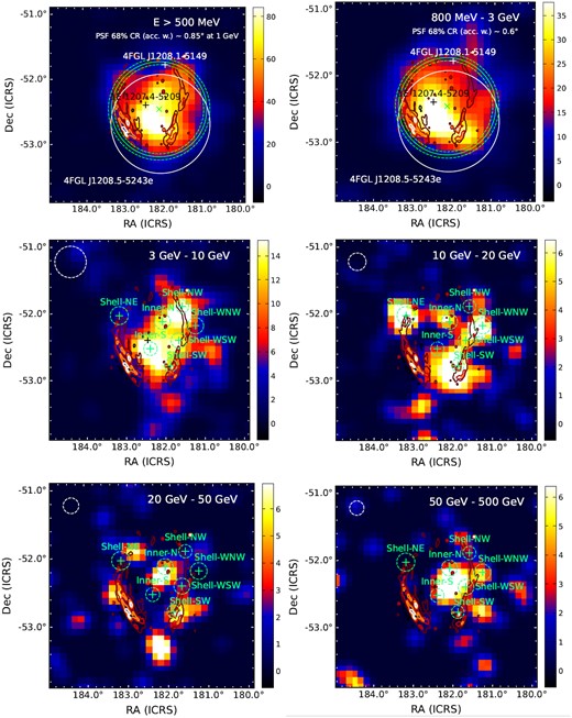
TS maps of the γ-ray emission in a region of 5° × 3° size towards SNR G296.5+10.0 for different energy regimes as indicated in each panel. The contours shown correspond to the MOST radio emission at 843 MHz. The position of the radio-quiet X-ray pulsar 1E1207.4-5209 is marked with a black cross. The white dashed line in the top left corner corresponds to the LAT PSF (68 per cent CR). In the top panels, the white cross and solid line refer to the 4FGL-DR3 catalogued source’s position and extension (68 per cent CR). The green lines and crosses stand for the results obtained from our analysis, as explained in Sections 2.2 and 3.3.
As commented in Section 2.2 above, we performed a detailed energy study above 3 GeV to characterize the morphology of the γ-ray source. Initially, we fitted a normalized spatial template from the remnant radio shell at 843 MHz to the LAT data. As a reference for these template fits, see the contours depicted in Fig. 4. However, the model did not represent the data better than a Gaussian extended source, with TS ≈ 80 compared to a TS ≈ 185 for the Gaussian model (both referenced to the null hypothesis, i.e. only background: TS = 0). Also, we fitted both an inner point source at the locations discussed in Section 2.2 and the radio shell spatial template, and resulted in a TS ≈ [106–116] depending on the position of the source without improving the log probability of the Gaussian source model. Nonetheless, more than one source could still be contributing to the observed γ-ray emission. As can be seen in Fig. 4, we cannot rule out that the detection of γ-ray emission may come from one or more background sources observed in the radio band, located in the field of view. In particular, those sources near the position R.A. =182|${_{.}^{\circ}}$|0, Dec. =−52|${_{.}^{\circ}}$|2 are coincident with one of the γ-ray emission peaks observed above 20 GeV (see both bottom panels in Fig. 4).
In the second approach explained in Section 2.2, we fitted separately a set of putative point sources over the cells of a grid with 0|${_{.}^{\circ}}$|24 spacing. The recursive fitting process finishes in two situations: (1) when the log-likelihood of the (global) ROI model is equal to or greater than the maximum if a single extended source is considered, and (2) when no sources with TS ≳ 16 can be fitted within a cell. Then, we only retained those positionally coincident with (or within) the SNR radio shell. The latter procedure resulted in seven different putative sources: Inner-N, Inner-S, Shell-SW, Shell-NW, Shell-NE, Shell-WSW, and Shell-WNW. In the middle and lower panels of Fig. 4, we indicated the position of these sources with green crosses, while the green-dashed lines indicate the position error at a 95 per cent CL. The physical parameters obtained from the fitting process are listed in Table 3. The results will be discussed in Section 4.4.
| Name | Flux | Energy range | R.A. | Dec. | r|$_{68~\%}$| | Γ | TS |
|---|---|---|---|---|---|---|---|
| 10−11 [ph cm−2 s−1] | [GeV] | [°] | [°] | [°] | |||
| Inner-N | 4.54 ± 1.56 | [3–500] | 182.14 ± 0.04 | −52.16 ± 0.06 | 0.073 | 1.67 ± 0.24 | 27.3 |
| Inner-S | 5.05 ± 1.56 | [3–20] | 182.44 ± 0.05 | −52.57 ± 0.04 | 0.063 | 2.28 ± 0.34 | 26.0 |
| Shell-SW | 4.37 ± 1.47 | [3–40] | 181.93 ± 0.04 | −52.82 ± 0.04 | 0.060 | 2.02 ± 0.29 | 26.2 |
| Shell-NW | 5.37 ± 1.49 | [3–10] | 181.66 ± 0.04 | −51.93 ± 0.04 | 0.060 | 2.78 ± 0.56 | 25.3 |
| Shell-NE | 3.45 ± 1.37 | [3–20] | 183.20 ± 0.05 | −52.07 ± 0.07 | 0.083 | 2.11 ± 0.32 | 18.8 |
| Shell-WSW | 3.77 ± 1.36 | [3–40] | 181.73 ± 0.05 | −52.44 ± 0.05 | 0.072 | 2.04 ± 0.35 | 18.3 |
| Shell-WNW | 2.12 ± 0.91 | [5–200] | 181.33 ± 0.05 | −52.22 ± 0.06 | 0.076 | 1.62 ± 0.31 | 15.6 |
4 DISCUSSION
4.1 Distance and age
Based on a morphological comparison between two H i features probably linked to G296.5+10.0 near |$v=-16~{\rm km\, s}^{-1}$| and the optical/X-ray/radio emissions, Giacani et al. (2000) suggested a distance of |$2.1^{+1.8}_{-0.8}~{\rm kpc}$| for the remnant. They also found an H i hole at the same velocity, giving further support to their result.
In order to obtain an independent determination of the distance to the remnant, we employed the reddening-distance method based on the extinction model developed by Chen et al. (1999). The parameters necessary to apply this method (see e.g. Reynoso et al. 2006; Reynoso, Cichowolski & Walsh 2017) are the colour excess |$E(B-V)$| measured on the source, the total reddening in its direction along the line of sight up to the edge of the Galaxy, |${E(B-V)}_{\infty }$|, the distance from the Sun to the Galactic Plane, z⊙, and the scale height of the Galactic Plane absorbing dust, h.
For the first parameter, we assumed the standard relation between the optical extinction |$\rm {A_v}$| and the reddening as E(B − V) = |$\rm {A_v}$|/3.1. To obtain |$\rm {A_v}$|, we applied the |$\rm {A_v}$|–NH relation derived for SNRs (Güver & Özel 2009), |$N_{\rm H}=(2.21 \pm 0.09)\times 10^{21}~\rm {A_v}$|. We calculated the reddening |$E(B-V)$| using each NH found for the twelve regions towards the X-ray emission of the SNR (see Section 3.2). The second parameter, |${E(B-V)}_{\infty } \sim 0.1360 \pm 0.0041~{\rm mag}$|, was obtained from Schlafly & Finkbeiner (2011).6 For the other two parameters, we assumed that h = 117.7 ± 4.7 pc (Kos et al. 2014) and z⊙ = 19.6 ± 2.1 pc (Reed 2006). Replacing all parameters in the Chen et al. (1999) model, we estimated that the distance to G296.5+10.0 is in the range 1.3–1.5 kpc, closer than previous estimates (albeit marginally coincident within the uncertainties). This distance places G296.5+10.0 at the near side of the Carina Arm, approximately 250 pc above the Galactic Plane.
Several estimates of the age of G296.5+10.0 are found in the literature, all based on the Sedov–Taylor self-similar solution which connects the size and age of an SNR as
where E0 is the kinetic energy, ρ0 = μmHn0 the ambient density, μ the mean atomic mass per hydrogen particle, n0 the ambient particle density, and mH the mass of the hydrogen atom. Kellett et al. (1987) assumed E0/n0 = 1.5 × 1051 erg cm−3 and a distance of 1.5 kpc (i.e. R ∼ 17.6 pc) and obtained an age around 20 000 yr. Matsui, Long & Tuohy (1988) arrive at the same result but combining a different set of parameters: a distance of 2 kpc, n0 ∼ 0.08 cm−3 and E0 ∼ 7 × 1050 erg. Considering these discrepancies, Roger et al. (1988) assumed the same E0 as in Kellett et al. (1987) and allowed for different distances (in the range 1 and 2 kpc) and intercloud densities (0.08–0.24 cm−3) from the two previous studies. These authors obtained an age of 7000 yrs, with an uncertainty within a factor of 3.
We will adopt the same density and initial energy as in Kellett et al. (1987), and will assume a 10 per cent content of He in the ISM, which implies μ = 1.4. At the distance d ∼ 1.4 kpc estimated above, the mean radius of G296.5+10.0 is 15.5 pc. The age of the SNR, hence, turns out to be ∼14 000 yr, which is consistent with the expected age for a mature SNR, in agreement with the previous works.
4.2 X-ray properties of the plasma
Using six XMM–Newton observations, we performed the double subtracted-background process to display the full extension of the X-ray emission associated with G296.5+10.0 (see Section 3.1). Fig. 1 shows the X-ray distribution of the plasma in three energy bands: soft (0.4–0.6 keV), medium (0.6–0.9 keV), and hard (0.9–2.0 keV). Also, the figure displays white contours of the radio emission of the SNR at 843 GHz. As observed earlier with EXOSAT (Kellett et al. 1987), the X-ray emission is almost fully confined to the south-eastern part of the SNR, with a very faint contribution on the south-western side. This strongly asymmetric distribution of the X-rays emission is in contrast with the symmetric, bilateral shape of the SNR in the radio band. In spite of this difference, the high resolutions of our image and the MOST radio image used for comparison allow us to observe a close correlation between the brightest features in both spectral bands.
The XMM–Newton image also shows the X-ray hole pointed by Kellett et al. (1987) near the centre of the Eastern lobe, roughly at RA = 12h12m and Dec = −52°41′. An enlargement of this region is displayed in Fig. 5, where the hole is highlighted with a green ellipse. Kellett et al. (1987) reported two bright peaks surrounding the western edge of the X-ray hole. Rather than two peaks, we found an arc-shaped feature with clumpy X-ray emission running parallel to the radio contours. We notice that the X-ray hole is actually observed in the MOST radio image as well therefore we will hereafter refer to it as the ‘Eastern hole’. The bright arc surrounding the hole to the East also has a radio counterpart and, noticeably, is the only region of the SNR emitting hard X-rays (seen as a white spot in Fig. 1). In the rest of the SNR, the X-ray emission is dominated by a mix of the soft and medium bands.
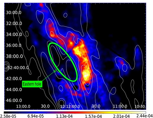
False coluor image of the X-ray emission towards G296.5+10.0 using the six observations from XMM–Newton. The radio emission at 843 GHz is represented with white contours at 0.03, 0.16, 0.24, and |$0.32~{\rm mJy\, beam}^{-1}$|. The green ellipse represents the Eastern hole described in Section 4.2. The coordinates are R.A.(J2000) and Dec.(J2000). The North is up and the East is to the left.
Our spectral study confirms that the plasma has a thermal origin, with an electron temperature uniform along the different X-ray emitting regions. The mean electron density ne can be inferred from the emission measure EM defined as |${\rm EM} = \int {n_{\rm e}\, n_{\rm H}}\, {\rm d}V$| assuming a locally uniform ne within each volume V, a cosmic abundance for hydrogen and helium ([He]/[H] = 0.1) and adopting the relation |$n_{\rm e} \sim 1.2\, n_{\rm H}$|. To compute EM, we apply the equation |${\rm EM} = \frac{4\pi }{10^{-14}}\, {\rm Norm}\, d^2$|, with d = 1.4 kpc (see Section 4.1) and replacing Norm by the normalization parameters listed in Table 2 for the different fitted spectra. We will furthermore assume that each region can be represented by an ellipsoidal volume Vell with a dimension along the line of sight equal to the minor axis, and the volume actually occupied by the plasma is |$V =f\, V_{\rm ell}$|, where f is the filling factor. Hence, ne can be expressed in terms of f as |$n_{\rm e} = \sqrt{1.2~{\rm EM}/V_{\rm ell}}\, f^{-1/2}$|. The density values are quite uniform throughout the different plasma regions, varying within the limited range of 0.11f−1/2 to 0.19f−1/2 cm−3 (see Table 2). We estimated the average ne to be ∼(0.16)f−1/2 cm−3, in close agreement with the results found in Kellett et al. (1987). Using the total unabsorbed flux estimation for the twelve regions, the total plasma has an X-ray luminosity of |$1.2 \times 10^{34} ~{\rm erg}\, {\rm s}^{-1}$|.
4.3 Comparison of the X-ray emission with the ISM distribution
To explore the contribution of the ISM to the X-ray emission, in this section we will analyse the H i distribution towards the SNR G296.5+10.0 from ATCA observations reprocessed as explained in Section 2.3. Adopting the Galactic rotation model of Fich, Blitz & Stark (1989), we find that the distance of 1.4 kpc estimated above for G296.5+10.0 corresponds to a radial velocity of |$-11\,{\rm km}\, {\rm s}^{-1}$| concerning the Local Standard of Rest (LSR). Hence, although a visual inspection of the data cube reveals that H i emission is detected from vLSR = −60 to |$+260\,{\rm km}\, {\rm s}^{-1}$|, we will focus on the limited range [|$-21, -7]\,{\rm km}\, {\rm s}^{-1}$|, where the emission most likely to be associated with G296.5+10.0 is expected to be found.
Fig. 6 displays the H i distribution between −20.78 and |$-7.58\,{\rm km}\, {\rm s}^{-1}$|, with MOST radio contours overlaid. We have not used the X-ray contours at this stage to keep a representation of the SNR full size, since the XMM–Newton image does not cover the northern part of the shell. Hence, although we aim to compare the ISM distribution with the X-rays emission, the radio image will help us identify the H i structures and radial velocities likely to be associated with the SNR. In each of the nine frames, we integrated two consecutive velocity channels and indicate the velocity of the first one. As can be seen from Fig. 6, there is extended, strong emission corresponding to the Carina arm crossing the two limbs at the northern part of the radio shell in different velocity channels. It is striking how this strong H i emission drops abruptly inside the SNR radio shell. Within this emission, we notice an arc-shaped feature about 20 arcmin-long in the frames from −14.18 to |$-10.88\,{\rm km}\, {\rm s}^{-1}$|, which seems to close the gap between the two limbs of the radio shell at the north. A careful inspection of the H i data cube shows that this feature, hereafter feature ‘A’, is found specifically between −13.35 and |$-10.05\,{\rm km}\, {\rm s}^{-1}$|. In Fig. 7, we present an image of the H i integrated into this last velocity range. The central velocity of Feature A is about |$-11.7\,{\rm km}\, {\rm s}^{-1}$|, in excellent agreement with the velocity expected for material at the distance of the SNR, 1.4 kpc. Based on this coincidence and the remarkable morphological correlation displayed in Fig. 7, we suggest that Feature A is very likely related to G296.5+10.0.
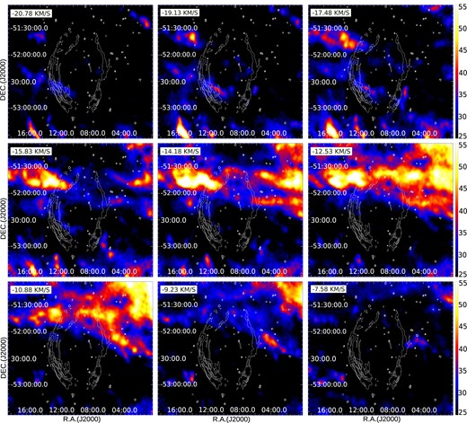
Colour image of the H i distribution around the SNR G296.5+10.0 in the velocity range from −20.78 to |$-7.58\,{\rm km}\, {\rm s}^{-1}$|. Each frame shows the emission integrated over two consecutive velocity channels, indicating the velocity of the first channel in the upper left corner. The colour scale is in units of |${\rm K}\,{\rm km}\, {\rm s}^{-1}$|. The white contours at 0.03, 0.16, |$0.24~{\rm mJy\, beam}^{-1}$| represent the radio emission at 843 GHz. The North is up and the East is to the left.

Colour image of the H i distribution around the SNR G296.5+10.0 integrated between −13.35 and |$-10.05\,{\rm km}\, {\rm s}^{-1}$|. The colour scale is in units of |${\rm K}\,{\rm m}\, {\rm s}^{-1}$|. The white contours at 0.03, 0.16, |$0.24~{\rm mJy\, beam}^{-1}$| represent the radio emission at 843 GHz. The North is up and the East is to the left.
According to Fig. 6, there is very little H i emission towards the southern part of G296.5+10.0. However, there is an H i structure in the frames from −20.78 to |$-15.83\,{\rm km}\, {\rm s}^{-1}$|. This cloud appears to be crossing the middle of the south-eastern part of the shell, very close to the Eastern hole. Inspecting the data cube, we confirmed that this cloud can be seen within the range from −21.60 to |$-16.65\,{\rm km}\, {\rm s}^{-1}$|. To compare the distribution of the atomic material with the X-ray band in more detail, Fig. 8 shows a close-up of the H i emission between −21.60 and |$-16.65\,{\rm km}\, {\rm s}^{-1}$| in the vicinity of the Eastern hole. As in Fig. 6, each frame displays two consecutive channels integrated and the velocity of the first one is indicated. The H i structures are on colour scale, the X-ray emission in white contours and the Eastern hole is enclosed with a green ellipse. In Fig. 8, the H i structure is clearly observed as an elongated cloud (hereafter cloud ‘B’) about 40 arcmin in size. Assuming a distance of 1.4 kpc, we have estimated for cloud B a total H i mass of about 80 M⊙ with a volume density nH ∼ 20 cm−3. The northern end of cloud B is projected onto the Eastern hole and its surrounding arc-shaped ridge. In the lower frames, cloud B is brighter beyond the X-rays outermost contour, showing a good morphological correlation with the ridge. Such correlation suggests a possible association between cloud B and the SNR X-rays emission. Kellett et al. (1987) proposed that the enhanced X-ray emission of the arc-shaped ridge may originate from the SNR shock front interaction with a dense cloud, leaving the dense core of the cloud as a region with a hole in the X-ray band. They also argue that the emission from shocked material could be too soft to penetrate the ≥1021 cm−2 of the Galactic absorption material in the line of sight, generating the Eastern hole.
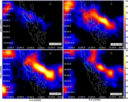
Colour image of the H i distribution around the SNR G296.5+10.0 in the velocity range from −21.60 to |$-16.65\,{\rm km}\, {\rm s}^{-1}$|. Each frame displays the emission integrated over two consecutive velocity channels. The velocity of the first channel is indicated in the bottom right corner. The colour scale is in units of |${\rm K}\,{\rm km}\, {\rm s}^{-1}$|. The white contours represent the XMM–Newton image of the X-ray emission associated with the SNR between 0.4–2.0 keV. The green ellipse indicates the Eastern hole mentioned in Section 4.2. The North is up and the East is to the left.
The detection of cloud B in this work may lend support to the cloud evaporation origin for the Eastern hole and the surrounding ridge as suggested by Kellett et al. (1987). However, it is not clear that cloud B is at the same distance as G296.5+10.0 since, although departures up to |${\sim}7\,{\rm km}\, {\rm s}^{-1}$| in velocity caused by turbulence are tenable (e.g. Reynoso et al. 2004), higher differences are found between the velocities where cloud B appears and the systemic velocity expected for the SNR (|$\sim -11\,{\rm km}\, {\rm s}^{-1}$|). Besides, our spectral analysis is in conflict with the hypothesis proposed by Kellett et al. (1987). Regions #2, #4, and #5 in the south-eastern radio limb, which coincide with the ridge surrounding the Eastern hole and the filament upwards, present enhanced abundances of Ne and Fe as compared to other regions in the SNR shell. This means that the X-ray emission from the ridge must be dominated by ejecta rather than arising from an evaporating swept-up ambient cloud.
The neutral gas distribution does not explain the strong asymmetries in the X-ray emission observed in G296.5+10.0. We do not find outstanding differences between the H i emission around the eastern and western lobes, neither at velocities compatible with the distance of the SNR nor in the foreground gas. This latter result is in agreement with the uniform values of NH measured in our spectral analysis throughout the different X-ray emitting regions (see Table 2). To get a more comprehensive picture of the ISM, we include data from the infrared (IR) space telescope Akari to survey the cold dust distribution. In Fig. 9, we display the emission at 140 |$\mu$|m (red) overlaid with the MOST radio emission at 843 MHz (green) and the X-ray plasma (blue). The image reveals a clear, albeit weak, increase of the IR emission towards the Eastern lobe of the SNR, while the Western lobe appears isolated. This difference, not observed in the rest of the IR frequencies (65, 90, and |$160\,\mu{\rm m}$|), is the only hint to explain the enhanced X-ray emission to the East. However, the metallicity at the brightest regions of the Eastern lobe, higher than in other regions, argues against a dominant influence of the ISM in the X-ray emission. The evidence gathered in this paper suggests that the explanation should be sought for reasons intrinsic to the SNR.
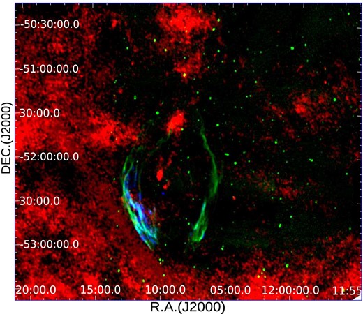
Composite image of the infrared emission at 140 |$\mu$|m (red), the radio emission at 843 MHz (green), and the X-ray plasma (blue). The North is up and the East is to the left.
4.4 The origin of the γ-ray emission
The large size of G296.5+10.0 and its hard γ-ray spectrum (with no hints of cut-off or attenuation at tens of GeV), together with the resolution attained by Fermi-LAT above few GeVs of energy, offers an opportunity to study spatial variations in the remnant’s γ-ray emission and its spatial correlation with the emission in other spectral bands.
In this work, we analyse fourteen years of accumulated Fermi observations and study the γ-ray emission in the energy range from 500 MeV to 500 GeV. As explained in Section 3.3, we found seven putative point sources (Inner-N, Inner-S, Shell-SW, Shell-NW, Shell-NE, Shell-WSW, Shell-WNW) and listed their physical parameters in Table 3.
Fig. 4 (described in Section 3.3) shows that the LAT γ-ray emission at energies below ∼3 GeV seems to arise from the interior of the remnant. For the energy range from [3–10] GeV, the γ-ray emission is mainly concentrated on the Inner-S and Shell-NW regions. In contrast, several γ-ray peaks can be observed in the [10–20] GeV regime. These are located towards the Shell-NE, the Shell-WSW, and the Shell-SW regions. In the energy range from 20 to 50 GeV, the γ-ray emission peaks close to the Inner-N and Shell-SW regions and marginally with part of the Shell-NE one. Finally, from 50 to 500 GeV, the LAT emission is positionally correlated with the Inner-N and Inner-S regions.
The γ-ray emission from [0.8–3] GeV partially follows the radio emission at the south-eastern part of the radio shell, with a γ-ray peak located at (R.A., Dec.)J2000 = (12h9m31s, −52°43′43″), inside the SNR and close to the X-ray pulsar. In Section 4.3, we identified two H i structures that may be related to G296.5+10.0. Feature A is closing the gap between the two radio arcs at the north, while cloud B crosses the radio and X-ray emission at the middle of the south-eastern part of the radio shell. To analyse if this γ-ray emission could be explained through the hadronic mechanism driven by the interaction between the SNR and dense ambient gas, we performed a composite map of radio/X-ray/γ-ray bands with the contours of these H i clouds overlaid. Fig. 10 shows the radio emission at 843 GHz (in red), the X-ray plasma between [0.4–2] keV (in green), and the γ-ray emission between [0.8–3] GeV (in blue). The yellow contours correspond to the H i emission integrated between −13.35 and |$-10.05\,{\rm km}\, {\rm s}^{-1}$| (see Fig. 7), and the white contours represent the emission integrated from −21.60 to |$-16.65\,{\rm km}\, {\rm s}^{-1}$|. The white arrows indicate the boundaries of feature A and cloud B, respectively. From Fig. 10, we note that feature A, as well as the rest of the neutral gas associated with the Carina arm, lies not only far from the γ-ray maximum but also does not match even the weakest γ-ray emission regions. Therefore, it is difficult to associate these H i features with the γ-ray origin. Cloud B, on the other hand, extends from the SW of the γ-rays peak to the bright arc-shaped ridge that surrounds the Eastern hole and reaches the outer edge of the radio shell. The hadronic scenario requires heavy nuclei in the ISM to act as targets for the high-energy particles leaving the SNR shock front. The detection of cloud B indicates that ambient clouds are present and could be interacting with the SNR. However, the low mass and density of cloud B, together with its offset position relative to the γ-rays peak between [0.8–3] GeV, cast doubts on a hadronic origin for the latter emission. In addition, the required heavy nuclei are provided by molecular gas, which is usually associated with cold dust. Fig. 9 shows that the IR emission towards the SW of the SNR is diffuse and uniform, with no counterpart whatsoever with the H i features. This implies that the detected neutral clouds are unlikely to trace potential molecular clouds. In all, there are not enough arguments to defend the hadronic model to account for the γ-rays emission in this energy interval. Nonetheless, molecular line observations in the direction of Cloud B would be desirable to bolster or discard this hypothesis. We also made a comparison of Cloud B with the emission from 3 to 500 GeV, but there was no significant morphological correlation with the γ-ray putative sources.
![Composite image of the emissions in radio continuum at 843 MHz (red), in X-rays between [0.4–2.0] keV (green), and in γ-rays between [0.8–3] GeV (blue). The overlaid contours show two H i structures discussed in Section 4.3: feature A and cloud B. The yellow contours, at 90, 100, 110, and $112~{\rm K}\, {\rm km}\, {\rm s}^{-1}$, correspond to the H i emission integrated between −13.35 and $-10.05\,{\rm km}\, {\rm s}^{-1}$. The white contours, at 96, 101, and $110~{\rm K}\, {\rm km}\, {\rm s}^{-1}$, represent the H i emission integrated from −21.60 to $-16.65\,{\rm km}\, {\rm s}^{-1}$. The external limits of feature A and cloud B are indicated with white arrows. The North is up and the East is to the left.](https://oup.silverchair-cdn.com/oup/backfile/Content_public/Journal/mnras/528/2/10.1093_mnras_stad3921/1/m_stad3921fig10.jpeg?Expires=1749146923&Signature=nZMAmWKmkOxDoUCb8k9sjrTlCxZcayIsJDo5TlU5~aVGLqrrXC9LiM0OXG9rK28IlKVEEjhTneLVscTJMJalcmtYkXz3v71zX2YttDYuZ12qrVbxLVR~gT30Q~Fj7EXASNcve1-kyJmdSSUg1KZjlEj0DELTZFGpw59wlS7ERhJIkpnUmo-xJggui0tHVU-IgcToJ2Xc2mJD6V~LWSSQTDk9OgxKWT-uvYM0n8Mj1QLXB5N9ur4dWptAevTmaQMbf37fuKOEtgJDe-X-I0St8SWYEns8LJ3GjtlwCx-7ywGd7rtafXEi-b7I8-cOoO5D1r5-BCmLTwpwMsiiuGn0pg__&Key-Pair-Id=APKAIE5G5CRDK6RD3PGA)
Composite image of the emissions in radio continuum at 843 MHz (red), in X-rays between [0.4–2.0] keV (green), and in γ-rays between [0.8–3] GeV (blue). The overlaid contours show two H i structures discussed in Section 4.3: feature A and cloud B. The yellow contours, at 90, 100, 110, and |$112~{\rm K}\, {\rm km}\, {\rm s}^{-1}$|, correspond to the H i emission integrated between −13.35 and |$-10.05\,{\rm km}\, {\rm s}^{-1}$|. The white contours, at 96, 101, and |$110~{\rm K}\, {\rm km}\, {\rm s}^{-1}$|, represent the H i emission integrated from −21.60 to |$-16.65\,{\rm km}\, {\rm s}^{-1}$|. The external limits of feature A and cloud B are indicated with white arrows. The North is up and the East is to the left.
The LAT GeV spectral indices obtained for Shell-NE, Shell-NW, Shell-WSW, and Shell-SW regions (see Table 3) are similar to each other (within errors), with values ranging approximately from 2 to 2.8, while the Shell-WNW region presents a harder index. The latter, however, is only marginally coincident with the radio limb of the remnant and also is the point-like source with the worst statistics (TS < 16). In order to investigate the origin of the γ-ray emission in what follows, we will compare the spectral indices obtained here with those observed at radio wavelengths (α). If the radio and γ-ray emission trace the same underlying particle population, the photon indices of radio and γ-ray emissions may follow the known correlations for π0 and e± bremsstrahlung (Γ = 2α + 1) or Inverse Compton (IC) scattering from leptons off the local photon fields (Γ = α + 1). To check this, we computed spectral indices in different areas over the SNR shell by applying the T–T plot technique on two radio images, at 1.38 and 4.85 GHz. Details on this technique, which has the advantage of being non-dependent on the background emission, can be found in Reynoso & Walsh (2015) and references therein. The data at 4.85 GHz were accessed from the PMN survey (Condon, Griffith & Wright 1993), while the image at 1.38 GHz was obtained as explained in Section 2.3. We found that the radio spectral indices for the regions over the shell (Shell-NE, Shell-NW, Shell-SW, and Shell-WSW) are 0.3 ± 0.2, 0.45 ± 0.30, 0.2 ± 0.45, and 0.25 ± 0.5, respectively.
Comparing the radio and γ-ray spectral indices obtained, we observe that GeV spectral indices for the cited regions are softer than predicted by either of the above-mentioned correlations. However, such behaviour is already observed for most SNRs in the first Fermi-LAT SNR catalogue (Acero et al. 2016). The deep survey carried out by Fermi-LAT established two general trends for the catalogued population of bright γ-ray SNRs differentiated by their gamma-ray spectra and physical characteristics: (1) a population of young and hard-spectrum (non-thermal X-rays) SNRs and (2) a population of older and brighter SNRs often interacting with dense gas in large molecular clouds. The radio/γ-ray indices obtained for the regions positionally correlated with the shell of the remnant agree best with those observed for the latter population (see Fig. 14 of Acero et al. 2016). The large errors obtained, however, prevent a clear association between the radio/γ-ray indices and these (i.e. ‘young’ and ‘interacting’) SNR subclasses. Also, emission from high-energy leptons cooled via synchrotron or IC mechanisms (Γ = α + 3/2) cannot be ruled out due to the large errors. The fact that the spectral index is softer for the GeV regime compared to the radio emission can be due to several reasons. For instance, the GeV and radio emission might not trace the same particle population, and underlying hadronic and leptonic populations might be present with different power law (PL) indices or might not follow a PL distribution, presenting breaks or other spectral features. Notwithstanding, a more detailed physical model is required to explain the origin of the γ-ray emission studied.
Concerning the Inner-N region, we found three potential counterpart candidates for the γ-ray origin. Fig. 11 shows the image of the X-ray emission using ROSAT archival data, overlapping with MOST radio contours in green color. Using the NASA/IPAC Extragalactic Database,7 we identified the X-ray source 2RXP J120827.7-521418 located at (R.A., Dec.)J2000 = (12h8m27|$.\!\!^{\rm {\mathrm{s}}}$|7, −52°14′17|${_{.}^{\prime\prime}}$|9) on the southern part of the green circle. There are also two radio sources: SUMSS J120840-520446 and WISEA J120805.90-521234.3. All three sources are indicated with arrows in Fig. 11. To compute spectral indices for the radio sources, we combined the map at 843 MHz with another high-resolution map at 147.5 MHz obtained with the Giant Metre Radio Telescope (GMRT; Intema et al. 2017). Fluxes were computed by fitting a Gaussian on each source allowing for a background level and taking their integrals. The spectral indices obtained are listed in Table 4.
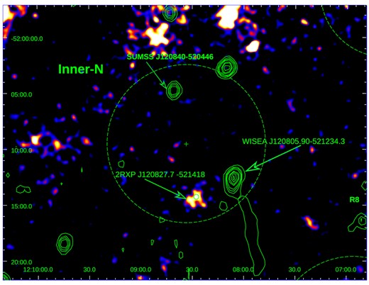
False color image of the X-ray emission inside the SNR G296.5+10.0 using ROSAT archival data. The overlapped green contours represent the MOST radio emission at 843 MHz. The green circle indicates the region Inner-N (95 per cent CL radius), with the two radio sources SUMSS J120840−520446 and WISEA J120805.90−521234.3, and the X-ray source 2RXP J120827.7-521418 mentioned in Section 4.4. The axes are R.A. and Dec. (J2000), with the North pointing up and East, to the left.
Radio point sources within the circle Inner-N.
| Source | Flux at | Flux at | Spectral |
|---|---|---|---|
| Name | 147.5 MHz | 843 MHz | Index |
| [mJy] | [mJy] | α | |
| SUMSS J120840-520446 | 82 ± 3 | 25.3 ± 0.9 | 0.67 ± 0.04 |
| WISEA J120805.90-521234.3 | 406 ± 5 | 70 ± 2 | 1.01 ± 0.02 |
| Source | Flux at | Flux at | Spectral |
|---|---|---|---|
| Name | 147.5 MHz | 843 MHz | Index |
| [mJy] | [mJy] | α | |
| SUMSS J120840-520446 | 82 ± 3 | 25.3 ± 0.9 | 0.67 ± 0.04 |
| WISEA J120805.90-521234.3 | 406 ± 5 | 70 ± 2 | 1.01 ± 0.02 |
For the Inner S region, there is no radio counterpart. However, we found three confirmed AGNs and six AGN candidates within the green circle indicated in Fig. 4 (middle and lower panels).
Alternatively, the emission observed from the interior of the SNR might indicate the presence of a pulsar wind nebula associated with 1E 1207.4–5209 that dominates the γ-ray emission from the region at the highest energies examined (E > 50 GeV). However, the LAT γ-ray luminosity obtained is |$L_{\gamma } (E > 3~{\rm GeV}) > 1.1 \times 10^{32}\times (d/1.4\,\rm {kpc})$| erg s−1 (at 95 per cent CL), even if only considering the luminosity of the Inner-S region above 3 GeV of energy. Gotthelf, Halpern & Alford (2013) reported that the pulsar has a low spin-down luminosity with |$\dot {E} \sim 1.2 \times 10^{31}~{\rm erg\, s}^{-1}$|. Therefore, the results allow us to rule out that 1E 1207.4–5209 powers the emission observed. Also, none of the putative sources Inner-S or Inner-N appears to be significantly extended in our images, and no extended emission was observed at X-rays either.
4.5 Spectral energy distribution
In this section, we present a physical model of the non-thermal emission of G296.5+10.0, consistent with the available data at radio and gamma energies. The set of parameters assumed and derived for the model are listed in Table 5.
Parameters of the physical model for G296.5+10.0. We indicate with superscript (†) those parameters that are assumed and with (‡) those that are derived. (1) This work; (2) Roger et al. (1988).
| Parameter | Symbol | Value | Units |
|---|---|---|---|
| Distance to the source(1) | d | 1.4 | kpc |
| Age(2) | tSNR | 14 000 | yr |
| Expansion velocity (1) | vSNR | 600 | |${\rm km\, s^{-1}}$| |
| Internal radius of the shell(1) | Rin | 3.13 × 10¹⁹ | cm |
| External radius of the shell(1) | Rout | 4.78 × 10¹⁹ | cm |
| Total energy(2) | ESNR | 6 × 1050 | erg |
| Relativistic particles content(†) | qrel | 0.1 | – |
| Hadron-to-lepton ratio(†) | a | 200 | – |
| Magnetic field(†) | B | 25 | μG |
| Acceleration efficiency(‡) | ηacc | 1.5 × 10⁻⁶ | – |
| Cold matter density(†) | np | 0.26 | cm−3 |
| Temperature of photon field (†) | T | 2.73 | K |
| Injection spectral index(†) | p | 1.9 | – |
| Maximum energy of electrons(‡) | |$E_{\rm e}^{\rm max}$| | 1013 | eV |
| Maximum energy of protons(‡) | |$E_{\rm p}^{\rm max}$| | 1014 | eV |
| Hillas energy(‡) | |$E_{\rm Hillas}^{\rm max}$| | 1017 | eV |
As the shell of the remnant expands into the ISM, two shock fronts are generated: a forward radiative shock and a reverse adiabatic shock. The shock is adiabatic if the thermal cooling length is larger than the size of the acceleration region (see e.g. Abaroa, Romero & Sotomayor 2023). On the reverse shock, particles are accelerated to relativistic energies through a first-order diffusive shock mechanism. Subsequently, relativistic hadrons and leptons can cool through different processes and produce non-thermal radiation. The diffusive acceleration rate of the particles is given by (e.g. Protheroe 1999):
where e is the electric charge, Z the atomic number, c the speed of light, B the magnetic field, and E is the energy of the particle. The acceleration efficiency ηacc of the process can be calculated with the velocity of the SNR expansion, assuming Bohm diffusion: |$\eta _{\rm acc}=3\beta _{\rm sh}^2/8$|, where βsh = vsh/c, with vsh ∼ vSNR.
The volume of the shell with internal (Rin) and external (Rout) radii, where particles are accelerated, is calculated as |$\Delta V= 4\pi (R^3_{\rm out}-R^3_{\rm in})/3$|. The fraction of kinetic power of the expanding shell that is transferred to the acceleration of relativistic particles is qrel = 0.1, and we set the hadron-to-lepton ratio to a = 200, following rough estimates of Beresinsky & Zatsepin (1969) for the production of cosmic rays observed in our Galaxy, which are supposed to be mostly accelerated in SNRs. Since the shock wave propagates into the ISM at a non-relativistic velocity, the magnetic field and the density at the reverse shock will be amplified by a factor of ∼4, following the Rankine–Hugoniot relations (see e.g. Lamers & Cassinelli 1999).
The time-scales associated with cooling are related to the energy loss of the particles, dE/dt ≈ −E/tcool. The total cooling rate is
where ti represents each time-scale for the involved cooling processes. The maximum energy for each kind of particle can be inferred by looking at the point, where the acceleration rate equals the total cooling or escape rate. We obtain a maximum energy of ∼10 TeV for electrons and ∼300 TeV for protons. This energy is within the bounds imposed by the Hillas criterion, which, in our case, is satisfied (|$E^{\rm max}_{\rm e,p} < E^{\rm max}_{\rm Hillas}\sim 10^{17}\, {\rm eV}$|).
Radiative cooling arises from non-thermal processes resulting from the interaction of particles with ambient fields and matter (see Romero & Paredes 2011; Romero & Vila 2014, plus references therein for additional details on radiative processes). Since our model is lepto-hadronic, we calculate the following radiative processes numerically:
Synchrotron: interaction of electrons with the ambient magnetic field of the ISM.
Inverse Compton (IC): collision of relativistic electrons with photons of the cosmic microwave background (CMB).
Bremsstrahlung: Coulombian interactions between relativistic electrons and cold matter.
Proton–proton: collision of relativistic protons with cold matter.
The evolution of the distribution of relativistic particles is determined by the transport equation (Ginzburg & Syrovatskii 1964). We solve this equation numerically under steady-state conditions and in the one-zone approximation. In the injection function of the particles, the energy follows a power law with an exponential cut-off,
where p is the spectral index. The normalization constant Q0 is obtained from
where ΔV is the volume of the acceleration region, and |$E^{\rm max}_{\rm (e,p)}$| the maximum energy reached by protons and electrons.
Once we have the particle distributions, we calculate the spectral energy distribution (SED) for each of the relevant processes involved in cooling. Fig. 12 shows the SEDs of the SNR G296.5+10.0 that we have obtained with our model. We find that synchrotron is the dominant process for electrons, followed by IC with CMB photons, and by Bremsstrahlung. On the other hand, hadronic interactions give rise to emission at very high energies.
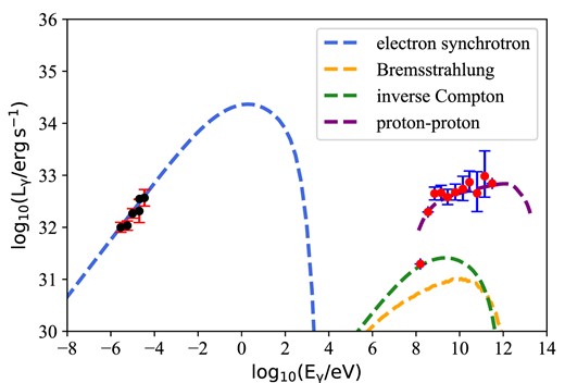
Spectral energy distributions of the SNR G296.5+10.0, for the different radiative processes that occur at the reverse shock of the expanding remnant. Black dots at the left correspond to the radio data, which can be explained by the electron-synchrotron mechanism; red dots are the right correspond to the gamma observations and can be explained by pp interactions. The parameters adopted for this model are listed in Table 5.
We found that the radio emission can be explained by electron synchrotron radiation under the hypothesis of a magnetic field |$B=25\, {\rm \mu G}$|, which is of the order of the magnetic field adopted by Zeng et al. (2021) in one of their scenarios. The γ-ray data can be explained by radiation through neutral pion decay, π0 → γ + γ, via proton–proton interactions, p + p → p + p + π0, assuming an ambient density of particles |$n_{\rm p}\sim 0.26\, {\rm cm^{-3}}$|. According to this model, the maximum luminosities are |$L{(E_{\gamma }=1{\, \rm eV})}\sim 5\times 10^{34}{\, \rm erg\, s^{-1}}$|, and |$L{(E_{\gamma }=10^{12}{\, \rm eV})}\sim 10^{33}{\, \rm erg\, s^{-1}}$|. The inverse Compton and Bremsstrahlung radiation mechanisms fail to provide sufficient power to explain the observations at very high energies.
5 SUMMARY
We have made use of the high spatial resolution provided by the XMM–Newton and Fermi telescopes to analyse the physical conditions of the high energy emitting plasma in the extended SNR G296.5+10.0. Our study was complemented with radio continuum observations to characterize the SNR, and H i line data to examine the distribution of the surrounding ISM.
The main findings can be summarized as follows:
The morphological study reveals that the X-ray plasma has a strongly asymmetric distribution between the south-east and south-west sides of the SNR, in contrast with the bilateral symmetry of the radio emission. However, the brightest features are coincident in both bands. In particular, we focus on a noticeable hole encircled by a bright, arc-shaped ridge of clumpy emission.
The spectral analysis confirms the thermal origin of the X-ray plasma, with an electron temperature homogeneous throughout the whole SNR. Some regions present enhanced abundances of N, Mg, and Fe, which suggest that the ejecta material is dominant.
The distance of 1.4 kpc estimated based on the reddening-distance method falls within the distance range estimated for the compact source 1E 1207.4–5209. It also locates G296.5+10.0 at the near side of the Carina Arm, with an age of ∼14 000 yr, typical for mature SNRs.
The average electron density of the plasma is ∼0.16 cm−3 and the X-ray luminosity is |$1.2 \times 10^{34} {\rm erg}\, {\rm s}^{-1}$|.
The analysis of the H i distribution gave little support to the hypothesis that the cloud evaporation model can explain the X-ray emission. This conclusion is also supported by the abundances resulting from the X-ray spectral analysis.
The analysis of Fermi data showed a hard unattenuated γ-ray spectrum and spatial variations in the GeV emission from the radio shell and interior regions. Although affected by large errors, the characteristics found for the LAT emission better agree with the trends observed for Fermi (hadronic) interacting SNRs compared to the young and middle-aged X-ray SNR subclass. An analysis of the SED also supports a hadronic origin to explain the emission at very high energies.
The results exclude that a pulsar wind nebula associated with 1E 1207.4–5209 powers the bulk of the γ-ray emission studied. Also, several compact radio and X-ray sources and AGNs or AGN candidates were found in the region and, together with 1E 1207.4–5209, may contribute to the total radiation observed at GeV energies.
ACKNOWLEDGEMENTS
LKE is supported by a CONICET fellowship. EMR, JAC, GER, and FG are members of the Carrera del Investigador Científico of CONICET, Argentina. JAC is a María Zambrano researcher fellow funded by the European Union -NextGenerationEU- (UJAR02MZ). This research was partially funded by CONICET grants PIP 112-201207-00226 and 112-201701-00604. JAC was supported by PICT 40-C-691 (UNRN). JAC and FG were supported by PIP 0113 (CONICET) and PICT-2017-2865 (ANPCyT) and PID2019-105510GB-C32/AEI/10.13039/501100011033 from the Agencia Estatal de Investigación of the Spanish Ministerio de Ciencia, Innovación y Universidades, and by Consejería de Economía, Innovación, Ciencia y Empleo of Junta de Andalucía as research group FQM-322, as well as FEDER funds. EM acknowledges support by grant P18-FR-1580 from the Consejería de Economía y Conocimiento de la Junta de Andalucía under the Programa Operativo FEDER 2014–2020. GER acknowledges financial support from the State Agency for Research of the Spanish Ministry of Science and Innovation under grants PID2019-105510GB-C31AEI/10.13039/501100011033/ and PID2022-136828NBC41/AEI/10.13039/501100011033/, and by ‘ERDF A way of mak- ing Europe’, by the ‘European Union’, and through the ‘Unit of Excellence María de Maeztu 2020–2023’ award to the Institute of Cosmos Sciences (CEX2019-000918-M). Additional support came from PIP 0554 (CONICET). EM is very grateful to Emma de Oña Wilhelmi for her help and suggestions (free of compensation) regarding the LAT data analysis.
DATA AVAILABILITY
The raw radio data at 1.4 GHz (continuum and H i line) are available in atoa.atnf.csiro.au/ATOA and can be accessed with the name project C738 (Green).
The X-ray data underlying this article are available in XMM-Newton Data Archive at http://nxsa.esac.esa.int/nxsa-web, and can be accessed with obsId indicated in Table 1.
All Fermi-LAT data are public and available at https://fermi.gsfc.nasa.gov/ssc/data/access/lat/.
Footnotes
See AtomDB for details of transitions, http://www.atomdb.org/index.php
The web site https://irsa.ipac.caltech.edu/applications/DUST/ provides a tool to obtain the reddening due to the dust for a given line of sight.
