


ABSTRACT
We propose a novel method to quantify the assembly histories of dark matter haloes with the redshift evolution of the mass-weighted spatial variance of their progenitor haloes, that is, the protohalo size history. We find that the protohalo size history for each individual halo at z ∼ 0 can be described by a double power-law function. The amplitude of the fitting function strongly correlates to the central-to-total stellar mass ratios of descendant haloes. The variation of the amplitude of the protohalo size history can induce a strong halo assembly bias effect for massive haloes. This effect is detectable in observation using the central-to-total stellar mass ratio as a proxy of the protohalo size. The correlation to the descendant central-to-total stellar mass ratio and the halo assembly bias effect seen in the protohalo size are much stronger than that seen in the commonly adopted half-mass formation time derived from the mass accretion history. This indicates that the information loss caused by the compression of halo merger trees to mass accretion histories can be captured by the protohalo size history. Protohalo size thus provides a useful quantity to connect protoclusters across cosmic time and to link protoclusters with their descendant clusters in observations.
1 INTRODUCTION
In the ΛCDM cosmological framework, cosmic structures originate from small primordial perturbations in the very early universe. These density fluctuations are then amplified by gravity and eventually form virialized structures called dark matter haloes. The evolution of cosmic structures proceeds hierarchically, where small haloes form first and subsequently assemble into larger haloes (White & Rees 1978; Mo, Van den Bosch & White 2010). In this scenario, gravitational potential wells associated with dark matter haloes provide conditions for the formation of galaxies, and so galaxies and haloes are expected to be tightly connected with each other. Therefore, understanding the assembly of dark matter haloes is a key step towards understanding the formation and evolution of galaxies (see Baugh 2006; Mo et al. 2010; Wechsler & Tinker 2018, for reviews). Dark matter haloes can be characterized from three perspectives.
The first is from the evolution of dark matter haloes with cosmic time. The formation and assembly of dark matter haloes can be well described by halo merger trees (Press & Schechter 1974; Lacey & Cole 1993; Somerville & Kolatt 1999). Such a tree structure grows from the descendant halo and splits into progenitor haloes backward in time recursively. Halo merger trees are informative but complex. It is therefore necessary to compress the information by extracting a small set of important features from full merger trees to describe halo assembly processes. A common practice is to focus on the main branch by recursively selecting the main progenitor. The halo mass growth along the main branch is commonly referred to as the mass accretion history (Wechsler et al. 2002; Zhao et al. 2009; Katsianis et al. 2023). A characteristic halo formation time can be defined as the highest redshift when the halo has accreted half of its final halo mass, or the redshift when the halo switches from fast accretion to slow accretion (Wechsler et al. 2002; Zhao et al. 2003a; Gao, Springel & White 2005; Wechsler et al. 2006).
The second perspective on dark matter haloes is their internal structure. Navarro, Frenk & White (1997) found that the density profile of dark matter haloes can be well described by a universal profile
where ρs is the density parameter and rs is a scaling radius. The asymptotic behaviour of this profile is ρ ∝ r−1 for r ≪ rs and ρ ∝ r−3 for r ≫ rs. In practice, a dark matter halo is restrained within a radius, Rvir, within which the mean density is equal to some chosen value, and the total mass within Rvir is defined as the halo mass, Mvir. Therefore, the NFW halo can be characterized with two other variables: the halo mass Mvir and the halo concentration c = Rvir/rs. In addition, dark matter haloes also exhibit non-spherical shape and the deviation from the spherical symmetry is more prominent for massive haloes (Jing & Suto 2002; Allgood et al. 2006). Finally, dark matter haloes also possess substructures from undissolved recent halo mergers (Moore et al. 1999; Yang et al. 2011; Jiang & van den Bosch 2016).
The last perspective on the halo population is from the spatial distribution, or the clustering of haloes. The spatial distribution of dark matter haloes can be characterized by the two-point correlation function and higher order statistics. The primary feature of halo clustering is the dependence on the halo mass, where massive haloes are more clustered than low-mass haloes. This phenomenon can be explained with a Gaussian initial density field and the extended Press–Schechter formalism (Mo & White 1996; Sheth, Mo & Tormen 2001). Moreover, the clustering of dark matter haloes also depends on their secondary properties, which is usually referred to as the halo assembly bias. Gao et al. (2005) first identified the dependence on halo formation time (see also Wechsler et al. 2006; Li, Mo & Gao 2008; Wang, Mo & Jing 2009; Lazeyras, Musso & Schmidt 2017; Mansfield & Kravtsov 2020; Barreira, Lazeyras & Schmidt 2021; Lazeyras, Barreira & Schmidt 2021; Wang et al. 2021b). Subsequent studies also find halo assembly bias caused by halo concentration, halo spin, and other properties (e.g. Gao & White 2007; Jing, Suto & Mo 2007; Wang et al. 2011). There are also attempts to detect such effects in observations, with mixed results (e.g. Wang et al. 2013a; Zu et al. 2021; Wang et al. 2022).
A comprehensive understanding of dark matter haloes requires not only knowledge from each perspective, but also relationships among properties in these three categories. In this respect, one important question is how halo structures are shaped by their assembly histories. Navarro et al. (1997) proposes a simple model that the difference in halo formation time and the time-dependence of cosmic density result in different halo concentrations. This model is further improved by subsequent studies (Bullock et al. 2001; Wechsler et al. 2002; Zhao et al. 2003a, b; Lu et al. 2006; Zhao et al. 2009; Diemer & Joyce 2019). Recently, Wang et al. (2020a) investigated the importance of merger events in shaping the halo concentration, and found that secular evolutions increase the concentration while sudden halo mergers reduce the concentration.
There is, however, one unresolved question on the relationship among halo structure, halo assembly history, and halo clustering. Jing et al. (2007) found that the halo assembly bias induced by the halo concentration is much stronger than the halo formation time for haloes above |$\gtrsim 10^{13}h^{-1}\rm {\rm M}_{\odot }$|. A detailed analysis in Mao, Zentner & Wechsler (2018) revealed that paired and unpaired cluster-size haloes have nearly identical mass accretion histories, and so there is no correlation between halo clustering and halo formation time, in contrast to results obtained by Chue, Dalal & White (2018). The question is: if the halo structure is determined by its assembly history, why the assembly bias of the halo concentration is absent in the mass accretion history for cluster-size haloes? One possible reason is that the assembly history alone cannot determine the structure of descendant haloes (see Ludlow et al. 2012). Another explanation is that the information about the halo assembly bias is lost during the data compression from halo merger trees to mass accretion histories. Wang et al. (2021b) proposed that the halo formation time is determined by both internal and external factors, which can produce opposite halo assembly bias effects with similar amplitudes for massive haloes. Therefore, the halo assembly bias effect of the halo formation time is very weak. In that case, a different compression method might be needed to retain the information about halo assembly bias.
In this study, we propose a new method to characterize the assembly of dark matter haloes, using the redshift evolution of protohalo sizes. This paper is organized as follows. Section 2 introduces the simulation data used in this study. Section 3 presents the redshift evolution of protohalo sizes and their relation to descendant haloes. Section 4 shows the assembly bias effect in terms of protohalo size. Finally, the discussion and summary of our main results are presented in Section 5.
2 DATA
In this study, we use the ELUCID simulation (Wang et al. 2013b, 2014, 2016; Tweed et al. 2017), which is a constrained N-body simulation to reconstruct the density field and formation history of our local Universe based on the Sloan Digital Sky Survey DR7 (York et al. 2000; Abazajian et al. 2009). This simulation has 30723 dark matter particles, each with a mass of |$3.09\times 10^8h^{-1}\rm M_\odot$|, in a box with a side length of |$500h^{-1}\rm Mpc$|. The simulation assumes a ΛCDM cosmology with Ωm = 0.258, |$\Omega _\Lambda =0.742$|, σ8 = 0.80, and h = 0.72.
Dark matter haloes are identified using the Friends-of-Friends (FoF) algorithm (Davis et al. 1985), and their masses are assigned as the total dark matter mass enclosed within a radius where the mean overdensity is 200 times of the critical density. The ELUCID simulation is complete for haloes to |$10^{10}h^{-1}\rm M_\odot$| up to z ∼ 8 (Wang et al. 2016). The concentration, c = Rvir/rs, of each FoF halo is estimated through their first moment, that is, |$R_1=\int _0^{R_{\rm vir}}4\pi r^3\rho (r)dr/M_{\rm vir}/R_{\rm vir}$|, whose relation to the concentration of NFW haloes can be expressed analytically (see Wang et al. 2024, for details). In each FoF halo, subhaloes are identified with the subfind algorithm (Springel et al. 2001), where the most massive subhalo is defined as the central subhalo and the remaining ones are satellite subhaloes. Subhaloes are linked to their progenitors and descendants using the code provided by Springel et al. (2005). The main branch of each subhalo is defined by recursively selecting the most massive progenitor. The peak halo mass, denoted as Mpeak, for each subhalo is defined as the maximum halo mass that it has achieved when it is a central subhalo. Finally, a protohalo is defined as the collection of all progenitor haloes at a given z > 0 that would end up in a common descendant halo at z = 0 (Wang et al. 2021a). Stellar masses are assigned to individual subhaloes following the stellar mass-halo mass relation in UniverseMachine based on Mpeak for each subhalo (see equation J1 in Behroozi et al. 2019). For each cluster at z = 0, we denoted its central stellar mass as |$M_{*, \rm cen}$|, and its total stellar mass as |$M_{*, \rm tot}$|. In this study, we use all dark matter haloes above |$10^{13}h^{-1}\rm M_\odot$| at z = 0 and trace their progenitor haloes above |$10^{10}h^{-1}\rm M_\odot$| to z = 8.
3 THE PROTOHALO SIZE HISTORY AND ITS RELATION TO DESCENDANT HALOES
3.1 Protohalo size and its redshift evolution
The assembly of a dark matter halo can be fully characterized by its merger tree. A snapshot of a halo merger tree at z > 0 gives a collection of haloes that will eventually end up in the halo at z = 0. Here we define this collection of haloes at z > 0 as a protohalo of its descendant halo at z = 0 (Wang et al. 2021a). We define the size of a protohalo as
where mi and xi are the mass and comoving position of the i-th progenitor halo, xcen is the centre of mass, and the sum is for all haloes above some mass threshold. We trace all the progenitor subhaloes for each descendant subhalo contained in the z = 0 main halo, from which we select all central subhaloes at a given redshift and use their M200c as mi to perform the summation in equation (2). For our main presentation, we choose the threshold to be |$10^{10}h^{-1}\rm M_\odot$| on the basis of ELUCID resolution. In Appendix A, we show that the ranking of protohalo sizes is nearly unaffected by the choice of the mass threshold. In addition, we also show in Appendix B that using the centre determined by a few dominating haloes to replace xcen does not alter the ranking of protohalo sizes significantly.
Fig. 1 shows the spatial distribution of member haloes for four protohaloes with similar descendant halo mass but with different sizes at z ∼ 2. The left and right two columns are two examples of protohaloes with large and small sizes, respectively. The three rows show projections in three directions, and the origins are chosen to be the centre of mass, xcen. Here the red, blue, and cyan circles represent haloes with mass above 1013, 1012, and |$10^{11}h^{-1}\rm M_\odot$|, respectively, and black dots are for haloes in the mass range of |$10^{10}-10^{11}h^{-1}\rm M_\odot$|. Despite the fact that these protohaloes will eventually collapse to form descendant haloes of similar masses at z = 0, their spatial distributions at high z are very diverse: the difference in linear size between the two extremes could be as large as a factor of ∼3. Large protohaloes (the left two columns) show diverse morphologies with abundant low-mass haloes, and their most massive haloes are not so different from other massive member haloes. In contrast, small protohaloes (the right two columns) are more compact with less abundant member haloes. They usually have a dominating halo, whose mass can be 10 times higher than the second one, located near the centre of mass. The diversity in protohalo sizes motivates us to investigate the information on halo assembly and structure encapsulated in this quantity.
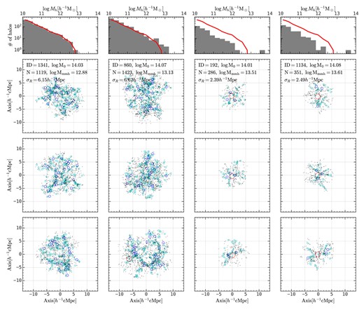
The member halo spatial distribution for four example protohaloes at z ∼ 2 with descendant halo mass around |$10^{14}h^{-1}\rm M_\odot$|. The left two columns are two examples with large protohalo sizes, and the right two columns are two examples with small protohalo sizes. The top panels show the halo mass distribution in each protohalo, and the halo mass distribution of the leftmost protohalo is overplotted on each panel in red solid curves for reference. The bottom three rows are for different projection directions. Haloes above 1013, 1012, and |$10^{11}h^{-1}\rm M_\odot$| are shown in red, blue, and cyan circles, and haloes within |$10^{10}-10^{11}h^{-1}\rm M_\odot$| are shown in black dots. The information about each halo, including the ID in ELUCID, the descendant halo mass, the richness, the halo mass of the most massive halo, the protohalo size, is shown in each row. This figure demonstrates the large diversity of spatial distribution of protohaloes at given descendant halo mass.
Fig. 2 shows the redshift evolution of the protohalo size of four haloes selected at z ∼ 0 with different halo masses. First of all, the redshift evolution of protohalo size is well behaved. It is nearly a constant above z ∼ 2, below which it rapidly collapses into a virialized halo by z = 0. Most strikingly, the turnover point occurs at z ∼ 2 across the whole halo mass range (see also Fig. 4). Secondly, the protohalo size above z ∼ 2 monotonically increases with the descendant halo mass. And the protohalo size is |$\sim 2\rm Mpc$| for group-size haloes, |$\sim 5\rm Mpc$| for ‘Fornax’-like haloes, |$\sim 6\rm Mpc$| for ‘Virgo’-like haloes, and |$\gtrsim 10\rm Mpc$| for ‘Coma’-like haloes. The correlation between protohalo size and the descendant halo mass is expected, because the formation of a more massive halo requires matter distributed over a larger volume at high z due to the homogeneity of the early universe. Finally, the redshift evolution of protohalo size is rather smooth.
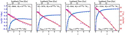
The protohalo size histories (cyan circles and blue solid lines on the left y-axis) and the mass accretion histories (magenta circles and red solid lines on the right y-axis) for four haloes selected at z ∼ 0. The circles are the histories calculated from each snapshot, and the solid lines are the fitting functions from equations (3) and (5). The vertical dashed lines show the half-mass time zhalf for each halo.
Fig. 2 also shows the mass accretion history, which is the halo mass evolution on the main branch, in magenta circles. The halo mass difference between current haloes and their main progenitors at z ∼ 8 is up to 3–5 dex, indicating that the mass accretion history based on the main branch only captures a small portion of the whole protohalo at high z. The dashed vertical line in each panel shows the half-mass redshift when the main progenitor has achieved half of its final halo mass. The small values of the half-mass redshift indicate that they only characterize the late-time evolution of haloes.
The protohalo size history and the mass accretion history are two ways to compress the halo merger tree into a one-dimensional function, and further compression may be achieved by fitting these histories with some simple parametric forms. Motivated by the two-stage evolution of protohalo size observed above, we use a double power-law function to fit its evolution from z ∼ 8 to z ∼ 0:
where Rc = R(zc) is the amplitude of the protohalo size history. If α > β, then R(z) ∝ zα for z ≪ zc and R(z) ∝ zβ for z ≫ zc. We assume prior ranges of α ∈ (0, 5) and β ∈ (− 1, 1) for α and β, respectively, and set zc = 2 as it is sufficient to fit the data (see Fig. 2). This functional form can accurately describe individual protohalo size history across the whole halo mass range probed according to our visual inspection.
Fig. 3 shows the dependence of fitting parameters on the descendant halo mass. Here one can see that the late-time slope α is around 1 and it has a marginal dependence on the descendant halo mass, with low-mass haloes tending to collapse slightly more rapidly. The early-time slope β is independent of the descendant halo mass, and has a median value of −0.2. Finally, the amplitude Rc has a power-law relation with the descendant halo mass, with a logarithmic slope of ∼0.39. In an ideal situation where descendant haloes form from a uniform density field, we expect dlog Rc/dlog M0 = 1/3 ≈ 0.33, which is close to our result here.
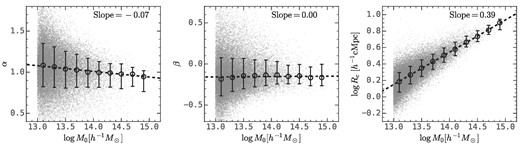
The scatter of the descendant halo mass and three parameters for the protohalo size histories in equation (3). The error bars show the median and the 16th−84th percentiles. The black dashed lines are the linear fitting functions to the median values, where the slope is labelled on each panel.
3.2 Relation to the structure of descendant haloes
Here, we first study the relation between the protohalo size history and the substructure of descendant haloes. We adopt the central-to-total stellar mass ratio to characterize the substructure, for the following reasons. First of all, this quantity is observable, so that the results obtained here can be related to observations. Secondly, the stellar mass used here is obtained according to the Mpeak of each subhalo (see Section 2) and this relation is well established at z ∼ 0 (Wechsler & Tinker 2018). Finally, Mpeak is less affected by the resolution of simulations, while other quantities for substructures, such as the subhalo mass, require high resolution for reliable estimates (Jiang & van den Bosch 2016).
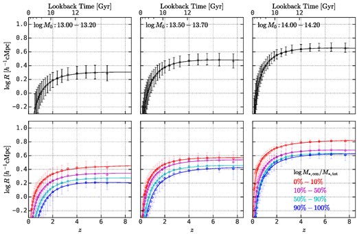
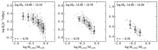
We find that the protohalo size history strongly correlates with the substructures of descendant haloes. Fig. 4 shows the average protohalo size evolution as a function of redshift with different descendant halo masses, log M0, where the error bars show the median and the 16th−84th percentiles and the solid lines are the fitting results of the double power-law function. In each bottom panel, descendant haloes are further divided into four subsamples according to their central-to-total stellar mass ratios, |$\log M_{*, \rm cen}/M_{*, \rm tot}$|, where the stellar mass is assigned using the empirical relations in UniverseMachine. At z > 2, the amplitude of the protohalo size history has a strong dependence on the central-to-total stellar mass ratio of descendant haloes, where haloes with higher |$\log M_{*, \rm cen}/M_{*, \rm tot}$| tend to have smaller protohaloes. Quantitatively, the difference in the protohalo size for haloes with the top-10 per cent and bottom-10 per cent central-to-total stellar mass ratios is about 0.2–0.3 dex, despite that the 1σ range of the protohalo size in each descendant halo mass bin is only ∼0.1–0.2 dex (see top panels).
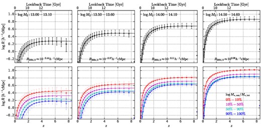
Top panels: The redshift evolution of protohalo size, R, in four halo mass bins. Bottom panels: In each halo mass bin, haloes are divided into four equal-size subsamples according to their |$\log M_{*, \rm cen}/M_{*, \rm tot}$|. The error bars show the median and the 16th−84th percentiles. This figure demonstrates the strong correlation between the protohalo size history and the |$\log M_{*, \rm cen}/M_{*, \rm tot}$| of descendant haloes.
A quantitative correlation analysis is presented in Fig. 5, which shows the relation between the parameters in equation (3) and the central-to-total stellar mass ratio, |$\log M_{*, \rm cen}/M_{*, \rm tot}$|, of descendant haloes in four narrow halo mass bins. The top panels show the results for the late-time slope α, where Spearman’s rank correlation coefficient is about 0.5 across the whole halo mass range. Descendant haloes with more dominating central galaxies tend to have steeper late-time slopes, indicating more rapid collapses of protohaloes to form descendant haloes. The panels in the middle row show results for the early-time slope β, whose correlation with |$\log M_{*, \rm cen}/M_{*, \rm tot}$| is negligible. Finally, the bottom panels show results for the amplitude of the protohalo size history, log Rc, where Spearman’s rank correlation coefficient is about 0.8. The difference in log Rc for haloes with the highest and lowest |$\log M_{*, \rm cen}/M_{*, \rm tot}$| is about 0.4 dex, compared to the 1σ width of log Rc in each halo mass bin, which is about 0.1–0.2 dex (see the top panels of Fig. 4). In addition, we find that the dependence of log Rc on log M0 and |$\log M_{*, \rm cen}/M_{*, \rm tot}$| can be described concisely by
As one can see from Fig. 6, the predicted log Rc matches the true log Rc well and the width for the 16th−84th percentiles is smaller than 0.1 dex.
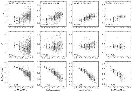
The correlation between the central-to-total stellar mass ratio, |$\log M_{*, \rm cen}/M_{*, \rm tot}$|, and the parameters in equation (3). Four columns are for different descendant halo mass bins, and the bin sizes are adjusted to be minimized while containing sufficient data points for statistical analysis. The top panels are for the late-time slope α, the middle panels are for the early-time slope β, and the bottom panels are for the amplitude log Rc. This figure demonstrates that the amplitude of the protohalo size history strongly correlates to the descendant central-to-total stellar mass ratio, as the correlation for the other two parameters is much weaker.
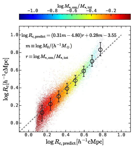
Accuracy of the amplitude of the protohalo size history, that is, log Rc, calibrated in equation (4). The x-axis is the prediction from the relation shown in the figure, and the y-axis is the true log Rc for each individual halo. The colour encodes the central-to-total stellar mass ratio. The error bars show the median and the 16th−84th percentiles. This figure shows that the log Rc calibrated against log M0 and |$\log M_{*, \rm cen}/M_{*, \rm tot}$| matches the true log Rc quite well.
In Appendix C, we restrained the protohalo as the collection of haloes that will end up in descendant subhaloes within the virial radius of the descendant main halo. This will effectively eliminate member haloes on the protohalo outskirt, since they are likely to become subhaloes outside the descendants’ virial radius. We found that the correlation between the protohalo size and the central-to-total stellar mass ratio is compromised but still as high as ≈0.6.
In Appendix D, we perform a similar analysis using the IllustrisTNG simulation (Pillepich et al. 2018a) and obtain similar results to Figs 4 and 5, which indicates that the results obtained here do not depend on the specific stellar mass-halo mass relation in UniverseMachine.
The relation between log Rc and |$\log M_{*, \rm cen}/M_{*, \rm tot}$| can be explained qualitatively. To begin with, the total mass in the region occupied by a protohalo is proportional to its final descendant halo mass. At a given descendant halo mass, protohaloes with larger sizes collapse at later times due to their relatively shallow gravitational potential. Therefore, the halo–halo merger events occur relatively late, and it becomes less probable for these late-accreted satellite subhaloes and their galaxies to be cannibalized by their central subhaloes and central galaxies. Consequently, these systems have more substructures, which results in low values of |$\log M_{*, \rm cen}/M_{*, \rm tot}$|.
Finally, Fig. 7 shows a moderate negative correlation between log Rc and the halo concentration, c, where high-concentration haloes have more compact protohaloes. The rank correlation coefficient is ≳ 0.5 for group-size haloes and decreases to 0.3 for cluster-size haloes. This result is consistent with the result in Wang et al. (2021b), where it was found that high-concentration haloes have higher overdensity in Lagrangian space.
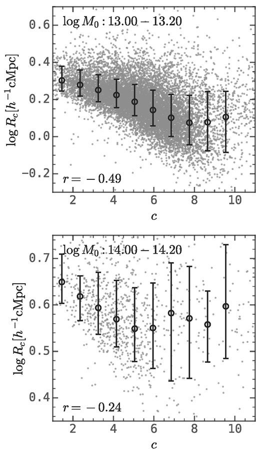
Relation between the amplitude of the protohalo size history, log Rc, and the halo concentration, c, in two halo mass bins. The erorr bars show the median and the 16th−84th percentiles. This figure shows that log Rc negatively correlates to c.
3.3 Relation to the mass accretion history
The hierarchical formation process of dark matter haloes can be fully characterized by halo merger trees. However, these tree-like structures are too complicated to use directly in the modelling of halo assembly. Some data compression is required. There have been attempts to extract compressed information from halo merger trees. A common method is to compress the halo merger tree into the mass accretion history (Wechsler et al. 2002; Zhao et al. 2003a). Further data compression can be done by defining some characteristic formation time, fitting the mass accretion history with some simple parametric forms, or using the principle component analysis technique (Wechsler et al. 2002; Gao et al. 2005; Wechsler et al. 2006; Li et al. 2008; Chen et al. 2020). Here we fit the mass accretion history with the functional form in McBride, Fakhouri & Ma (2009), which is
where M0 is the descendant halo mass at z = 0, and γ and δ are two free parameters. McBride et al. (2009) found that the combination, γ − δ, to be a useful parameter to characterize the mass accretion rate at low z, since
where z is close to zero. As shown in Fig. 2, this functional form can describe the simulated mass accretion histories reasonably well, but not in detail. One can use the fitting parameters to describe the overall properties of a mass accretion history, as we will do here. In principle, the fitting results can also be used to define a half-mass time as the highest z when the main progenitor has reached half of the final halo mass. The half-mass time defined in this way is not identical to zhalf obtained directly from the simulation data. We have checked that both definitions give similar results, and we will use the zhalf obtained directly from the data in our presentation. We note that there are other attempts to compress halo merger trees using state-of-the-art statistical tools (e.g. Forero-Romero 2009; Obreschkow et al. 2020).
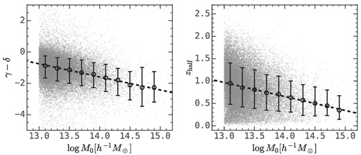
Our study proposes a new method which compresses a halo merger tree into a linear protohalo size history, and identifies that the most important quantity is the amplitude, log Rc. We emphasize that the protohalo size history is correlated with the mass accretion history, but encapsulates additional information of halo assembly that is missed in the mass accretion history. As shown in Fig. 8, the amplitude of the protohalo size history, log Rc, moderately correlates with the halo mass assembly time, zhalf, in the sense that smaller protohaloes tend to form earlier. This is expected: at fixed descendant halo mass, smaller protohaloes have deeper gravitational potential well, so that the member haloes can merge with each other in a shorter time-scale. Fig. 8 also shows that log Rc is in moderate correlation with γ − δ, which approximates the recent mass accretion rate (see equation (6)), in the sense that larger protohaloes tend to experience more rapid accretion at late times. We have also looked into other features extracted from the mass accretion history and found that zhalf exhibits the strongest correlation with log Rc.
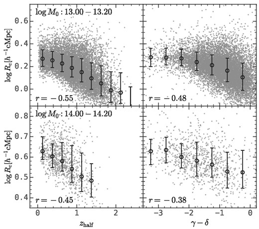
The relation between the amplitude of the protohalo size history, log Rc, and characteristic features of massive accretion history, including the half-mass time, zhalf, and the recent halo accretion rate, γ − δ, (see equation (6)). The error bars show the median and 16th−84th percentiles. This figure shows that the haloes with large protohalo sizes tend to form later and experience more rapid accretion than the haloes with small protohalo size.
The protohalo size history also encapsulates information on halo assembly that is missed in the mass accretion history. First of all, as one can see from Fig. 5, log Rc strongly correlates with the substructure of descendant haloes, while a similar analysis in Appendix E shows that the correlation between the mass accretion history and the substructure of descendant haloes is much weaker. Secondly, log Rc contains extra information about the halo concentration, c. To demonstrate it, we take the residual of log Rc and c conditioned on zhalf and plot their relation in Fig. 9. Here one can see that these two residual quantities are still moderately correlated, with Spearman’s coefficient about 0.3. The last manifestation is in the halo assembly bias effect, as we will show in Section 4.
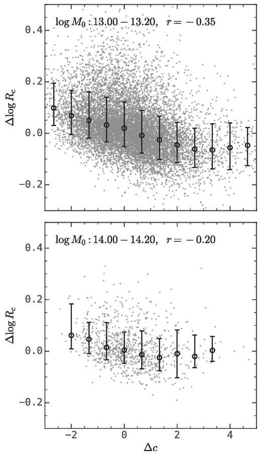
The correlation between Δc and Δlog Rc in two narrow halo mass bins. Here, Δc and Δlog Rc are the difference between these two quantities and their median relation with respect to zhalf. The error bars show the median and 16th−84th percentiles. This figure demonstrates that the amplitude of the protohalo size history contains extra information about the descendant halo structure that is missed by the half-mass time.
Finally, it is noteworthy that the mass accretion history and the protohalo size history captures different stages of halo assembly. The mass accretion history primarily features the late-time evolution when a dominant progenitor halo emerges, since the characteristic halo formation times derived from the mass accretion history, such as the half-mass time and the time when the halo transits from fast accretion to slow accretion, are below z ≲ 2 for haloes above |$10^{13}h^{-1}\rm M_\odot$|. On the contrary, the protohalo size history features the early-time evolution prior to the collapse of the protohalo, which occurs at z ∼ 2. Therefore, the combination of these two quantities might give us a more complete picture of halo assembly.
4 HALO ASSEMBLY BIAS
Dark matter haloes are biased tracers of the underlying density field, and the square root of the ratio between the clustering strength of haloes and the underlying density field is defined as the halo bias. The halo bias primarily depends on halo mass, where massive haloes are more clustered (Mo & White 1996). In addition, the clustering of dark matter haloes also depends on their secondary properties, including shape, formation time, concentration, and spin. Such dependence is referred to collectively as the halo assembly bias (e.g. Sheth et al. 2001; Gao et al. 2005; Wechsler et al. 2006; Jing et al. 2007; Li et al. 2008; Mao et al. 2018). The existence of halo assembly bias implies the entanglement of secondary halo properties and their large-scale environments, and so an analysis of the halo assembly bias can help us better understand the formation of dark matter haloes.
Here, we study the assembly bias using the autocorrelation function estimated with
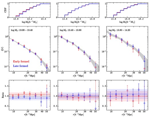
where DD(r) is the pair counts within a distance of r ± δr for the target sample, and RR(r) is the pair counts within the same distance for the random sample. We find a strong halo assembly bias effect caused by the amplitude of the protohalo size history, log Rc. As shown in Fig. 10, the autocorrelation function is higher for haloes with larger Rc compared with haloes with smaller Rc. Here the subsamples with large and small protohaloes are constructed based on their log Rc relative to the median relation shown in the right panel of Fig. 3. Their descendant halo mass distributions are nearly identical, as shown in the top panels. Their autocorrelation functions are presented in the middle panels of Fig. 10, where the red and blue error bars are the results for large and small protohaloes, respectively, and the grey shaded regions are the results for all the haloes in the same mass bin. The error bars in the bottom panels show the ratio between each subsample and the parent sample. The shaded regions show the mean ratio by averaging the ratios from 10 to 30 |$h^{-1}\rm Mpc$|, which is an estimate of the square of the relative bias (b2 = ξsubsample/ξparent). Here one can see that the bias factor between the 50 per cent of haloes with the largest Rc and the 50 per cent with the smallest Rc is about |$\sqrt{1.2/0.8}- 1\approx 22~{{\ \rm per\ cent}}$|, which is larger than the assembly bias caused by the half-mass time. According to the results obtained in Jing et al. (2007), the bias factor of the 20 per cent of haloes with the smallest zhalf is just about 10 per cent larger than that the 20 per cent with the largest zhalf, as is also shown in Appendix E. Note that the halo assembly bias reported here extends to |$\gtrsim 40\rm Mpc$|, although the error bars are large due to the limited simulation box size.
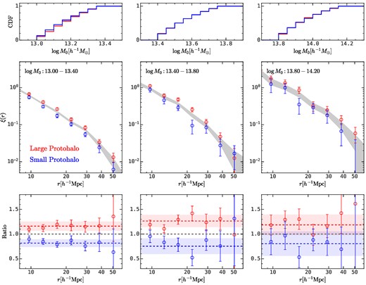
Top panels: The autocorrelation functions for dark matter haloes in three halo mass bins. The grey shaded regions are for all haloes in each halo mass bin. The red and blue error bars are for subsamples with ΔA above and below zero, respectively. Bottom panels: The ratio of the autocorrelation functions between two subsamples and the parent sample in each halo mass bin. The shaded regions show the average ratio from 10 to 30 |$h^{-1}\rm Mpc$| for each subsample. This figure shows the difference in the clustering strength for haloes with large and small protohaloes is about |$1.2/0.8-1\approx 50~{{\ \rm per\ cent}}$|.
Like the mass accretion history, the protocluster size history is not directly observable. However, as shown in Section 3.2, the central-to-total stellar mass ratio, |$\log M_{*, \rm cen}/M_{*, \rm tot}$|, is tightly correlated with Rc, and so can be served as an observational proxy. As a proof of concept, Fig. 11 shows the halo assembly bias manifested by |$\log M_{*, \rm cen}/M_{*, \rm tot}$|. Here the results are similar to the results we obtained using Rc in Fig. 10, indicating that the proxy is reliable.
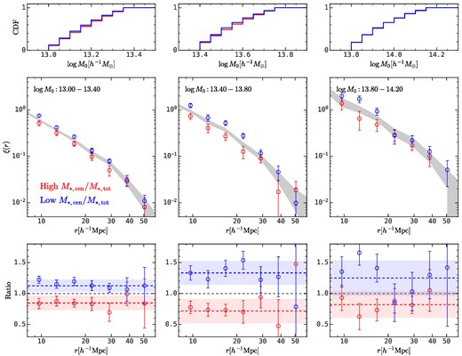
Similar to Fig. 10, except that the subsamples are divided according to their |$M_{*,\rm cen}/M_{*, \rm tot}$|.
Actually, halo assembly bias effects based on quantities like |$M_{*, \rm cen}/M_{*, \rm tot}$| have already been detected in observations. Zu et al. (2021) used the REDMAPPER cluster catalogue constructed from the SDSS DR8 to study the dependence of the halo assembly bias caused by the central stellar mass to halo mass ratio, where the halo mass is controlled using the weak gravitational lensing technique. They found that the large-scale bias for clusters with lower central stellar mass is 10 per cent higher than that of higher central stellar mass from both weak gravitational lensing and galaxy clustering results (Zu et al. 2022). Under the assumption that the relation between total stellar mass and halo mass of these clusters is sufficiently tight (Bradshaw et al. 2020), their detection is similar to the halo assembly bias effect exhibited by the amplitude of the protohalo size history approximated by the central-to-total stellar mass ratio. Moreover, they also found a difference in the halo concentration between subsamples with large and small central stellar masses, indicating that the halo assembly bias exhibited by the protohalo size and by the halo concentration are related to each other, as shown in Fig. 7.
Finally, we note that the halo assembly bias effect is a manifestation of the entanglement between halo properties and the large-scale environment. Such effect is present for the halo concentration, c = Rvir/rs, but not for the half-mass time, zhalf (Jing et al. 2007; Wang et al. 2021b), nor the entire mass accretion history (see Mao et al. 2018, and Appendix F). This makes us wonder how the halo concentration ‘knows’ the large-scale environment without the assembly history ‘knowing’ it. In this study, we find that the protohalo size history exhibits a strong halo assembly bias effect. Besides, Appendix F further demonstrates that paired and unpaired cluster-size haloes have nearly identical mass accretion histories, but different protohalo size histories, which suggests that the environmental effects on halo formation must have been lost during the data compression from halo merger trees to mass accretion histories, and such effects are captured by the protohalo size history.
5 DISCUSSION AND SUMMARY
5.1 Implications for connecting protoclusters and clusters
A protocluster, by definition, is a set of dark matter haloes, as well as their associated baryons, at z > 0 that will eventually collapse into a common cluster-size dark matter halo at z = 0. In other words, protoclusters are protohaloes whose descendant halo mass is |$\gtrsim 10^{14}h^{-1}\rm M_\odot$|. Such objects are well defined in simulations where we can track their evolution. However, it is non-trivial to identify protoclusters in observation due to the difficulty in predicting the fate of those high-z objects. A feasible way is to characterize true protoclusters in simulations with a few features, such as the galaxy number overdensity, and find objects in the observation that exhibit similar properties (e.g. Chiang, Overzier & Gebhardt 2013). This kind of method is straightforward but their performance is difficult to assess since they rely on the visual inpsection. A more advanced way is to develop an automatic structure finding algorithm, which can be trained in simulations and applied to mock surveys for performance assessments (e.g. Stark et al. 2015; Wang et al. 2021a).
How to build a reliable connection between protoclusters and present day clusters is, therefore, an essential step in understanding the formation of clusters, and the evolution of cluster galaxies. Conventionally, such connections are built using masses of protoclusters and descendant clusters. For each identified protocluster, the mass can be estimated according to proxies such as the number overdensity of tracers and the total mass within the protocluster. However, the mass alone cannot capture the diversity of protocluster, as shown in Fig. 1 (see also Lovell, Thomas & Wilkins 2018).
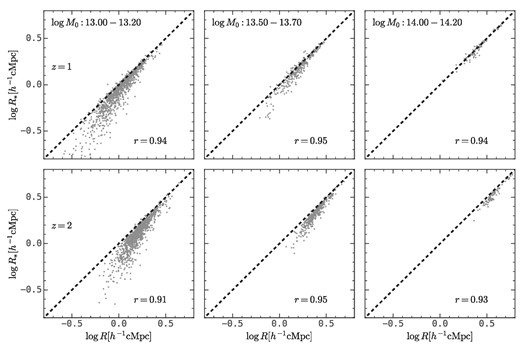
We find that the protocluster size, which is defined in the same manner as the protohalo size, is an excellent secondary property to connect protoclusters across cosmic time and their descendant clusters at z ∼ 0. The left and middle panels of Fig. 12 show the correlation between the central-to-total stellar mass ratio of descendant clusters and the protocluster size at z ∼ 2 and z ∼ 8, respectively. Here one can see that these correlations are tight, with Pearson’s correlation coefficients as high as ∼0.86(0.77) for z ∼ 2(8). The right panel shows the correlation between the sizes of protoclusters at z ∼ 2 and z ∼ 8, and the correlation coefficient is about 0.9.
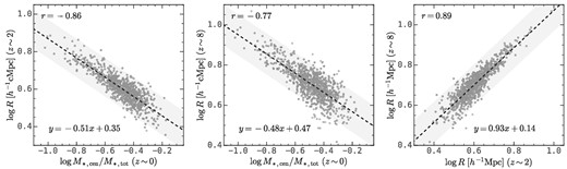
Property correlation for protoclusters at z ∼ 2 and z ∼ 8 and descendant clusters at z ∼ 0 with descendant halo mass between |$10^{14}h^{-1}\rm M_\odot$| and |$10^{14.2}h^{-1}\rm M_\odot$|. Left and middle panels: The correlation between the |$\log M_{*,\rm cen}/M_{\rm *,tot}$| of descendant clusters and the size of their protohalo at z ∼ 2 and z ∼ 8, respectively. Right panel: The correlation between the sizes of protohaloes at z ∼ 2 and z ∼ 8. The black dashed lines are the linear fitting results and the shaded regions are the ±0.1 dex regions. Pearson’s correlation coefficients are presented at the top-left corner of each panel. This figure demonstrates that the protohalo size serves as an excellent secondary property to connect protoclusters across cosmic time and their descendant clusters through their |$\log M_{*, \rm cen}/M_{*, \rm tot}$|.
Thus, the protocluster size can be used to refine the connections of protoclusters across cosmic time and to local galaxy clusters. This refinement may be referred to as the secondary cluster–protocluster connection. Observationally, the usefulness of this refinement relies on the fact that the protocluster size and the central-to-total stellar mass ratio of descendant haloes are tightly correlated and that galaxy groups and protoclusters can be reliably identified from observations (Yang et al. 2007; Wang et al. 2020b; Yang et al. 2021; Li et al. 2022). However, our findings also pose a challenge to the identification of protoclusters from observation. As we have shown, the size difference between protoclusters of similar descendant mass can be as high as ∼0.5 dex. This corresponds to a factor of 100.5 × 3 ≈ 30 in volume, and suggests that protocluster finders based on overdensities within a fixed aperture may produce a biased protocluster catalogue. Clearly, for a density-based protocluster finder, such bias needs to be quantified using realistic mock catalogues (Stark et al. 2015; Wang et al. 2021a).
5.2 Summary
We propose a novel method to characterize the assembly of massive dark matter haloes using the protohalo size history. Our main findings are summarized as follows
the protohalo size history exhibits two-stage evolution: an early-time static phase and a late-time collapsing phase. These features can be captured by a double power-law function with a characteristic redshift at z = 2 in the halo mass range between |$10^{13}h^{-1}\rm M_\odot$| and |$10^{15}h^{-1}\rm M_\odot$|. The late-time slope α and the early-time slope β are nearly independent of the descendant halo mass, while the amplitude log Rc positively correlates with the descendant halo mass with a slope of ∼0.39 (see Figs 2 and 3).
At a given descendant halo mass, the amplitude of the protohalo size history, log Rc, strongly correlates to the central-to-total stellar mass ratio, |$\log M_{*, \rm cen}/M_{*, \rm tot}$|, of the descendant haloes, with smaller protohaloes evolving to descendant haloes that are more dominated by central galaxies. There is also a moderate correlation between the late-time slope and |$\log M_{*, \rm cen}/M_{*, \rm tot}$|, in the sense that more rapid collapsing produces a more dominating central galaxy (see Fig. 4 and Appendix E).
The protohalo size history correlates with the mass accretion history, but also encapsulates critical information about halo assembly that is missed by the mass accretion history. This is reflected in its tight correlation with the central-to-total stellar mass ratio, |$\log M_{*, \rm cen}/M_{*, \rm tot}$|, and its correlation with halo concentration when zhalf is fixed (see Figs 8, 5, and 9).
The amplitude of the protohalo size exhibits a strong halo assembly bias effect, in that descendant haloes of a given mass with larger protohalo sizes are more strongly correlated. A similar assembly bias effect is found for the central-to-total stellar mass ratio of descendant haloes, due to its strong correlation to the protohalo size. However, the halo assembly bias exhibited by the half-mass time is much weaker at the massive end. This indicates that the information about halo assembly bias is lost during the data compression from halo merger trees to the mass accretion histories, and this information is captured by the protohalo size histories (see Figs 10 and 11 and Appendix E).
The sizes of protoclusters at z ∼ 2 to z ∼ 8 are all strongly correlated with the central-to-total stellar mass ratio of their descendant clusters at z ∼ 0. The sizes of protoclusters at different redshifts are also strongly correlated to each other, which indicates the protocluster size is a useful quantity to link protoclusters at high-z to their descendants at z ∼ 0 (see Fig. 12).
Our results suggest that the protohalo size history may provide a new avenue to study the halo assembly history and its relation to galaxy formation and evolution. The amplitude of the protohalo size history has a reliable observational proxy, which is the central-to-total stellar mass ratio. In contrast, observational proxies for the commonly used mass accretion histories are not as reliable, especially for massive haloes (Wang et al. 2023). The protohalo size history also encapsulates information about the halo assembly that is missed in the mass accretion history, as is manifested by the halo assembly bias effect. Finally, the protohalo size can be used as a secondary parameter, in addition to mass, to link protoclusters across cosmic time, and to link protoclusters to descendant clusters at z ∼ 0. This will help us to better understand the assembly of galaxy clusters and the evolution of their member galaxies, when applied to the existing and upcoming high-z galaxy surveys, such as MAMMOTH (Cai et al. 2016, 2017), COSMOS-Webb (Casey et al. 2023), PFS (Greene et al. 2022), and MOONS (Maiolino et al. 2020).
ACKNOWLEDGEMENTS
The authors acknowledge the Tsinghua Astrophysics High-Performance Computing platform at Tsinghua University for providing computational and data storage resources that have contributed to the research results reported within this paper. KW and YP are supported by the National Science Foundation of China (NSFC) Grant Numbers 12125301, 12192220, 12192222, and the science research grants from the China Manned Space Project with NO. CMS-CSST-2021-A07. HW is supported by NSFC Grant Number 12192224.
The computation in this work is supported by the HPC toolkit hipp (Chen & Wang 2023), ipython (Perez & Granger 2007), matplotlib (Hunter 2007), numpy (van der Walt, Colbert & Varoquaux 2011), scipy (Virtanen et al. 2020), astropy (Astropy Collaboration et al. 2013, 2018, 2022). This research made use of NASA’s Astrophysics Data System for bibliographic information.
6 DATA AVAILABILITY
The data underlying this article will be shared on reasonable request to the corresponding author.
References
APPENDIX A: PROTOHALO SIZES USING DIFFERENT HALO MASS LIMITS
Here, we examine the impact of the halo mass limit used to estimate the protohalo size and the central-to-total stellar mass ratio of descendant haloes.
The top panels of Fig. A1 show the scatter plot of the amplitude of the protohalo size history, that is, log Rc, estimated using progenitor haloes above |$10^{10}h^{-1}\rm M_\odot$| (the limit adopted in the main body of the paper) and |$10^{11}h^{-1}\rm M_\odot$|, and Spearman’s rank correlation coefficients are presented in each panel. Here, one can see that a higher halo mass limit will cause an underestimation of the protohalo size. This is expected since massive haloes are more biased and prefer to live in central parts of protohaloes. This underestimation is moderate for group-size descendant haloes and negligible for cluster-size descendant haloes. Most importantly, the rank correlation coefficient between different halo mass limits is ∼0.96 in the lowest descendant halo mass bin and even higher for more massive bins, indicating that such underestimation effects do not alter the relative ranks of log Rc for these haloes.
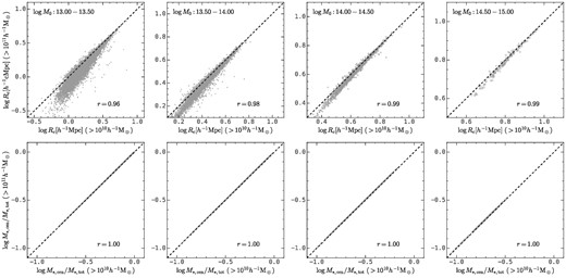
The comparison of the amplitude of the protohalo size history (top panels) and the central-to-total stellar mass ratio (bottom panels) with the halo mass limit as |$10^{10}h^{-1}\rm M_\odot$| (x-axis) and |$10^{11}h^{-1}\rm M_\odot$| (y-axis). Spearman’s rank correlation coefficients are presented on each panel. This figure shows that a higher halo mass limit causes an under-estimation of the amplitude of the protohalo size history, log A, for haloes with low mass and small protohalo size, but little damage to the rank of log Rc. The impact on the central-to-total stellar mass ratio, |$\log M_{*, \rm cen}/M_{*, \rm tot}$| is negligible.
The bottom panels of Fig. A1 shows the central-to-total stellar mass ratio of descendant haloes, that is, |$\log M_{*, \rm cen}/M_{*, \rm tot}$|, using all subhaloes with peak halo mass above |$10^{10}h^{-1}\rm M_\odot$| and |$10^{11}h^{-1}\rm M_\odot$|, respectively. There is nearly no difference between these two quantities, indicating again that subhaloes with low peak halo mass have a negligible contribution to the total stellar mass.
APPENDIX B: PROTOHALO SIZES USING DIFFERENT CENTRING METHODS
Here, we examine the impact of the protohalo centring on the protohalo size calculations. To this end, we use four different methods to determine the protohalo centre xcen
using the mass of centre of all haloes above |$10^{10}h^{-1}\rm M_\odot$| in each protohalo, which is used in the main body of the paper;
using the position of the most massive halo above |$10^{10}h^{-1}\rm M_\odot$| in each protohalo;
using the mass of centre of top-2 most massive haloes above |$10^{10}h^{-1}\rm M_\odot$| in each protohalo;
using the mass of centre of top-3 most massive haloes above |$10^{10}h^{-1}\rm M_\odot$| in each protohalo.
In the latter two cases, if the number of haloes above |$10^{10}h^{-1}\rm M_\odot$| in the protohalo is smaller than the required number, we use all the available haloes.
Fig. B1 shows the scatter of the protohalo size estimated with different centring methods in four halo mass bins and three redshift snapshots. In each panel, the x-axis is the protohalo size calculated with the first centring method, and the y-axis shows those with the other three methods with vertical shifts for clarity. The dashed lines in each panel are the one-to-one reference lines. Spearman’s rank correlation coefficients for the protohalo sizes from different centring methods are presented on each panel. Here one can see that the first centring method produces the minimal protohalo size by design, as the other three methods will overestimate the sizes. Moreover, this overestimation effect has some general trends. First of all, the amplitude of the overestimation decreases with n, which is expected. Secondly, the protohalo sizes are more overestimated for larger protohaloes, which can be seen from that the deviation from the reference line is larger for larger x-values. Thirdly, such overestimation effects are larger for high-z protohaloes, which can be seen from the decreasing rank correlation coefficients with increasing redshift. Similarly, the overestimation effect is larger for protohaloes with massive descendant haloes. In summary, the overestimation effect is stronger in situations where the protohaloes are less likely to be dominated by a few massive haloes. Nevertheless, the rank of of the protohalo size is largely preserved, since the rank correlation coefficients are ≳ 0.85 even when only the most massive halo is used.
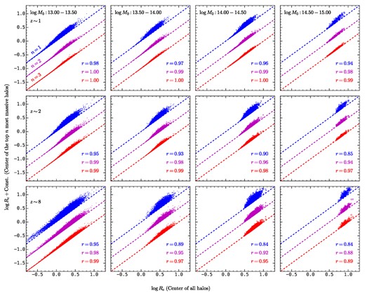
The comparison of protohalo sizes calculated with different centres. The x-axis is the protohalo size calculated with the centre of mass. The y-axis is the protohalo size calculated with the centre of mass for n most massive haloes in the protohalo, where n = 1 (blue), 2 (magenta), and 3 (red). Spearman’s correlation coefficients between two protohalo sizes are shown on each panel in the corresponding colour. This figure demonstrates that centring with a few most massive haloes will overestimate the protohalo size, and the overestimation is larger for situations without dominating haloes, such as large protohaloes, high-z protohaloes, and protohaloes with massive descendant halo mass. Nevertheless, the rank of the protohalo size is largely preserved, which is manifested by the high values of Spearman’s correlation coefficients.
APPENDIX C: PROTOHALO SIZES USING DIFFERENT SUBHALO MEMBERSHIP DEFINITION
In the main text, we define a protohalo as the collection of progenitor haloes of all subhaloes in the descendant FoF halo. Alternatively, we can define a protohalo as all of the progenitor haloes that will end up in descendant subhaloes that are enclosed within the virial radius of the descendant halo at z = 0. Here we considered three different common halo radius defined with different density threshold values: Rvir defined with the threshold density in Bryan & Norman (1998), R200m defined with the threshold density as 200Ωmρcrit, and R200c defined with the threshold density as 200ρcrit. The bottom panels of Fig. C1 show the comparison of protohalo sizes at z = 2 using different definitions. Note that the dependence of protohalo size on descendant halo mass is eliminated by taking the residual with respect to the median log R–log M0 relation. The protohalo sizes defined with additional descendants’ halocentric distance constraint are smaller than that defined with all descendant subhaloes in the descendant FoF halo. This is expected since the progenitor haloes of the subhaloes on the descendant halo’s outskirt prefer to locate in the outer region of the protohalo, so that excluding these progenitor haloes will consequently reduce the protohalo size. Nevertheless, these protohalo sizes with different definitions still strongly correlate to each other.
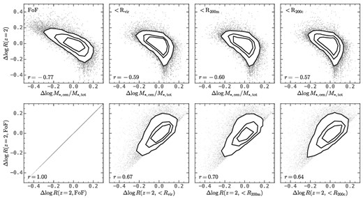
The top panels show the relation between the residual protohalo size at z = 2 and the residual central-to-total stellar mass ratio at z = 0 for different subhalo membership definitions for all descendant haloes above |$10^{13}h^{-1}\rm M_\odot$|. Similarly, the bottom panels show the comparison of the protohalo sizes at z = 2. The contour lines show encloses 50 per cent, 70 per cent, and 90 per cent of all haloes. The first column includes all subhaloes in each FoF halo, and the second column includes only subhaloes within Rvir. Similarly, the third and fourth columns include only subhaloes within R200m and R200c, respectively.
The top panels of Fig. C1 show the relation between the protohalo size and the central-to-total stellar mass of descendant haloes with the dependence on halo mass eliminated by taking the deviation from the median value in narrow halo mass bins. Note that the calculation of |$M_{*,\rm tot}$| only includes subhaloes within the corresponding radius. After eliminating subhaloes out of halo radius, the correlation coefficient between the protohalo size and the central-to-total stellar mass ratio is reduced but still as high as ≈0.6.
APPENDIX D: RESULTS FOR THE ILLUSTRISTNG SIMULATION
The IllustrisTNG project comprises various cosmological galaxy formation simulations with different box sizes and resolutions (Marinacci et al. 2018; Naiman et al. 2018; Nelson et al. 2018; Springel et al. 2018; Pillepich et al. 2018a, b; Nelson et al. 2019). Here we use the one with the largest box size, which is called the TNG300 simulation, for better statistics. TNG300 simulates the formation and evolution of dark matter haloes and galaxies in a box with a side length of |$205h^{-1}\rm Mpc$|. The dark matter particle mass is about |$5.9\times 10^7\rm M_\odot$|, and the mass for each gas particle is about |$1.1\times 10^7\rm M_\odot$|.
Fig. D1 shows the protohalo size evolution as a function of redshift in three descendant halo mass bins. The evolution is very similar to that obtained from the ELUCID simulation (see Fig. 4. The bottom panels show the protohaloes size evolution binned with the central-to-total stellar mass ratio of descendant haloes, |$\log M_{*, \rm cen}/M_{*, \rm tot}$|. Here one can see that protohaloes with the top-10 per cent and bottom-10 per cent |$M_{*, \rm cen}/M_{*, \rm tot}$| values differ in their size by 0.2–0.3 dex, despite the fact that the 1σ range of the protohalo size is only 0.1–0.2 dex (see top panels). In addition. Fig. D2 shows the correlation between log Rc and |$\log M_{*, \rm cen}/M_{*, \rm tot}$| in three halo mass bins, as well as Spearman’s rank correlation coefficient, which is about 0.8. These results show that the tight correlation between the protohalo size and the central-to-total stellar mass ratio of descendant haloes is also present in the IllustrisTNG simulation, where the stellar mass in each halo is obtained through hydrodynamical simulation instead of empirical modelling.
Similar to Fig. 4, except for the TNG300 simulation.
Similar to the bottom panels of Fig. 5, except for the TNG300 simulation.
Fig. D3 shows the comparison of protohalo size calculated with equation (2) and that weighted by the stellar mass of all progenitor galaxies, which is
where m*, i and x*, i are the stellar mass and position of the i-th progenitor galaxy. Here one can see that the protohalo sizes calculated using these two different ways are highly correlated to each other, despite that the size calculated using stellar mass is systematically smaller than that of halo mass for small protohaloes, which is caused by the non-constant stellar mass to halo mass ratio (Behroozi et al. 2019).
The comparison of protohalo size calculated with halo mass (x-axis) and stellar mass (y-axis) in TNG300 at z = 1 and z = 2. Spearman’s rank correlation coefficients are labelled at the lower right corner of each panel. This figure demonstrates that the protohalo sizes calculated using halo mass and stellar mass are highly correlated to each other, despite that the size calculated using stellar mass is systematically smaller than that of halo mass for small protohaloes.
APPENDIX E: RESULTS FOR THE MASS ACCRETION HISTORY
Here, we perform similar studies on the mass accretion history as we did on the protohalo size history in Section 3 and Section 4.
Fig. E1 shows the dependence on descendant halo mass for γ − δ in equation (5) and the half-mass time zhalf, and the relations to the central-to-total stellar mass ratio, that is, |$\log M_{*, \rm cen}/M_{*, \rm tot}$|, are presented in Fig. E2. Here one can see that both γ − δ and zhalf moderately correlate with |$\log M_{*, \rm cen}/M_{*, \rm tot}$| for group-size haloes. Haloes with more dominating central galaxies tend to form earlier and have lower recent accretion rates. The correlation becomes negligible for cluster-size haloes, which is consistent with the results in Wang et al. (2023). Neither of the parameters describing the mass accretion history has as a tight relation to |$\log M_{*, \rm cen}/M_{*, \rm tot}$| as the protohalo size history shown in Fig. 5.
Similar to Fig. 3, except for γ − δ and zhalf.
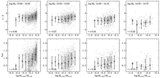
Similar to Fig. 5, except for γ − δ and zhalf.
Fig. E3 shows the halo assembly bias effect exhibited by the half-mass time zhalf. The signal is rather weak, which is consistent with the results obtained in previous studies (see Gao et al. 2005; Jing et al. 2007; Mao et al. 2018).
Similar to Fig. 10, except that subsamples here are divided according to their zhalf. This figure shows that the halo assembly bias from the halo formation time is negligible for massive haloes.
APPENDIX F: THE DEPENDENCE OF ASSEMBLY HISTORIES ON DESCENDANTS’ NEIGHBOUR COUNTS
In addition to the autocorrelation functions shown in Figs 10 and E3, we also use the method in Mao et al. (2018) to demonstrate the difference in the halo assembly bias effect exhibited by the mass accretion history and the protohalo size history for cluster-size haloes above 1014 h−1 M⊙. To begin with, we categorize haloes into different populations according to the number of another cluster-size halo within |$10h^{-1}\rm Mpc$| of the halo in question. Specifically, haloes are defined as isolated if the neighbour counts are zero. We also consider haloes with ≥1 neighbours and ≥2 neighbours. We then calculate the median mass accretion history, collapsed mass history, and protohalo size history in each category, as presented in Fig. F1. Here the collapsed mass history is defined as the total progenitor halo mass above fM0 with f = 0.02 as a function of redshift (e.g. Neto et al. 2007; Gao et al. 2008; Li et al. 2008; Ludlow et al. 2016). The fractional deviation relative to the results obtained for the parent halo sample is presented on the bottom panels. Note that the collapsed mass history drops below 0.02 M0 above z ≈ 3. This figure demonstrates that isolated haloes exhibit nearly identical mass accretion history and collapsed mass history to the paired haloes with more than one and two neighbours (Li et al. 2008). In contrast, paired haloes exhibit larger protohalo sizes than isolated haloes, and the fractional difference is about 5 per cent for haloes with ≥1 neighbours, and 10 per cent for haloes with ≥2 neighbours.
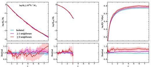
The top panels show the median mass accretion histories, collapsed mass history, and protohalo size histories for haloes above |$10^{14}h^{-1}\rm M_\odot$| and different numbers of neighbours within |$10h^{-1}\rm Mpc$|. The bottom panels show the fractional difference between three subsamples with different neighbour counts and the parent sample. The shaded regions show the standard deviation estimated from the bootstrap samples. This figure shows that the protohalo size history has a significant dependence on the surrounding environment of haloes, but such dependence for the mass accretion history and the collapsed mass history is negligible.
Fig. F1 contain different information about the halo assembly bias from Figs 10 and E3. The autocorrelation function characterizes the halo assembly bias on different scales, but it requires a further compression from a linear structure of history to a scalar, which are zhalf and log Rc in this case. In contrast, Fig. F1 compares the whole mass accretion history and protohalo size history for paired and unpaired haloes, but this comparison is made on the chosen scale, which is |$10h^{-1}\rm Mpc$| in our case. Therefore, Fig. F1 shows that not only zhalf, but also the whole mass accretion history contains no information about the halo assembly bias.
