


ABSTRACT
Stellar-mass black hole binary systems in the luminous X-ray states show a strong quasi-periodic oscillation (QPO) in their Comptonized emission. The frequency of this feature correlates with the ratio of a disc to Comptonized emission rather than with total luminosity. Hence, it changes dramatically during spectral transitions between the hard and soft states. Its amplitude is also strongest in these intermediate states, making them an important test of QPO models. However, these have complex spectra which generally require a disc and two separate Comptonization components, making it difficult to uniquely derive the spectral parameters. We build a new energy-conserving model of the accretion flow, SSsed model, which assumes a fixed radial emissivity but with a changing emission mechanism. This is similar to the agnsed model in xspec but tuned to be more suitable for stellar mass black holes. It uses a combination of the disc luminosity and temperature to constrain the inner radius of the (colour temperature corrected) blackbody disc, separating this from the more complex Comptonization spectra emitted inwards of this radius. We show a pilot study of this model fit to hundreds of RXTE spectra of the black hole binary XTE J1550 − 564. We show that the derived disc radius tightly anticorrelates with the central frequencies of the low-frequency QPO detected in the same observations. The relation is consistent with the quantitative predictions of Lense–Thirring precession of the entire inner Comptonization regions for the assumed system parameters. This supports the scenario that low-frequency QPOs are caused by Lense–Thirring precession.
1 INTRODUCTION
Stellar black hole binaries (hereafter BHBs) are characterized by large intensity variation and various spectral states. The spectral states are classified mainly based on the ratio of the soft spectral component to the hard spectral component. The soft component is well understood as multitemperature blackbody emission from the optically thick accretion disc, while the hard component is considered to be the result of inverse Compton scattering of seed blackbody photons from the disc by high-energy thermal or non-thermal electrons. The soft state is characterized by a dominant thermal disc component below several keV seen together with a weak power-law-like tail of photon index Γ ∼ 2.0–2.2 which extends beyond 500 keV (Grove et al. 1998; Gierliński et al. 1999). By contrast, the hard state is instead dominated by a hard (Γ ∼ 1.4–1.7) power-law with a thermal cutoff at around a few tens of keV to hundreds of keV. Therefore, there are at least two high-energy electron populations that can provide hard X-ray emission: one consists of steep non-thermal electrons, and the other consists of hot (approximately several tens of keV) thermal electrons. The former is most clearly important in the soft state, while the latter dominates the hard state.
The spectra in the intermediate states show a more complex structure. The intermediate states [further subdivided into the soft and hard intermediate states (SIMS and HIMS) e.g. Belloni et al. 2005; Remillard & McClintock 2006] have spectra in which both the disc and Compton tail are seen, but the tail is much stronger than in the soft state but much softer (Γ > 2.2) than in the hard state (e.g. Zdziarski et al. 2001; Życki, Done & Smith 2001; Gierliński & Done 2003). They can be fit either by two different Comptonizing plasmsas, or a single plasma which has a hybrid (thermal plus non-thermal) electron distribution such as the eqpair model1 by Paolo Coppi (e.g. Hjalmarsdotter, Axelsson & Done 2016)
The disc inner radius can be derived from fitting the expected sum of blackbody spectral models to the data for the expected disc emissivity using a non-relativistic (Shakura & Sunyaev 1973) or relativistic (Novikov & Thorne 1973) standard disc emissivity. These show that this inner radius is generally constant in soft state spectra, as expected if the disc extends down to the innermost stable circular orbit (ISCO) (e.g. the reviews by Done, Gierliński & Kubota 2007; Inoue 2022 and references therein). The SIMS spectra are likely consistent with a similar inner radius (e.g. Kubota, Makishima & Ebisawa 2001; Kubota & Makishima 2004). In contrast, the question of whether the disc reaches the ISCO or is truncated in the HIMS and hard state remains debated. Energetically, the dominant hard X-ray emission is most easily explained with a composite accretion flow, where the thin disc truncates at some radius larger than the ISCO, transitioning into an inner hot geometrically thick accretion flow. However, this is claimed to be inconsistent with the results on the inner radius derived from fitting the best current models of the reflected emission from an irradiated accretion disc (e.g. Wang-Ji et al. 2018).
The fast time variability offers an independent way to characterize the spectral states. Low-frequency quasi-periodic oscillations (LF-QPOs) are commonly observed in the Comptonization component in the HIMS, SIMS and bright hard state (Ingram & Motta 2019 and references therein). Several models have been suggested to explain the origin of LF-QPOs but the one which is currently most popular is the Lense–Thirring (hereafter LT) precession (Stella & Vietri 1998) of the entire hot Comptonization region inwards of the standard disc truncation (Ingram, Done & Fragile 2009, hereafter IDF09; Motta et al. 2014). This model could be tested by measuring the truncation radius between the disc and corona, and correlating it with the measured QPO frequency. However, it is difficult to measure the disc-corona truncation radius from the disc continuum in the states where the QPO is strongest as these typically show strong, complex Comptonization, making the disc parameters difficult to uniquely determine.
Here, we impose additional constraints from energy conservation in order to derive the disc radius across several hundreds of Rossi X-ray Timing Explorer (RXTE) data of a stellar BHB, XTE J1550 − 56 (Smith 1989). This is now a standard idea in fitting AGN spectra (Done et al. 2012; Kubota & Done 2018) but was first actually suggested for these complex intermediate state spectra in BHB (Done & Kubota 2006). We use this to trace the time evolution of the size of the Comptonizing corona for all spectral states, and compare it with the LF-QPO frequency seen in the same data sets. We show that the transition radius between the disc and Comptonization regions tightly anticorrelates with the LF-QPO centroid frequency, unlike the scatter (parallel tracks) seen in when plotting the LF-QPO against absolute flux. We show that the transition radius derived from the spectral modelling matches fairly well with the quantitative prediction of LT precession of the Comptonizing regions.
In Section 2, we present a summary of RXTE observations of XTE J1550 − 564 and an overview of its spectral and timing features. In Section 3, we describe the details of the new model. We analyse the spectral data with the new model and determine the disc-corona geometry for several spectral states in Section 4. In Section 5, we compare the result of spectral analyses to LF-QPO frequencies and discuss the validity of LT precession, and we summarize the results of our study in Section 6.
2 OVERVIEW OF SPECTRAL AND TIMING PROPERTIES OF XTE J1550–564
XTE J1550 − 564 is a well-studied transient BHB, with five outbursts which were extensively observed with RXTE. The system parameters are fairly well known, at |$d=4.4^{+0.6}_{-0.4}$| kpc, with orbital inclination angle i = 75° ± 4° and black hole mass M = 9.1 ± 0.6 M⊙, respectively (Orosz et al. 2002, 2011). The Galactic absorption column from X-ray spectral fits of NH=(7.5–10)× 1021 cm−2 (Tomsick, Corbel & Kaaret 2001; Miller et al. 2003; Corbel, Tomsick & Kaaret 2006) is similar to that expected along the line of sight of NH = 9 × 1021 cm−2(Dickey & Lockman 1990), and makes only a small impact on the spectrum above 3 keV measured by RXTE.
The first two outbursts showed large intensity variations, exhibiting all the states (soft, SIMS, HIMS, and hard state), together with strong LF-QPOs, while the latter three outbursts remained in the hard states indicating failed outbursts. Therefore, we focus on the first two outbursts in this study.
Fig. 1 shows the 3–20 keV PCA light-curve normalized to 1 PCU unit (top panel), and the corresponding time evolution of the hardness ratio (hereafter HR) of 6–20 keV count rate to the 3–6 keV count rate (middle panel). The first outburst is divided into two semi-outbursts, each of which is indicated by red and orange colours, and the second outburst is coloured in cyan. The central frequencies of fundamental QPO and its higher/lower harmonics are plotted in the bottom panel of Fig. 1, Type-C and Type-B QPOs marked with black circles and dark grey triangles, respectively, and Type-A and the other unclear structures marked with light grey crosses. Here, Type-C QPOs are typically observed, and show strong and narrow features with broadband, flat-topped noise. Their QPOs are well represented by Lorentzian. Type-B QPOs are also narrow and strong but without strong broad-band noise, and their structures are reproduced by Gaussian. Type-A QPOs are weak and broad features (Ingram & Motta 2019, and references therein).
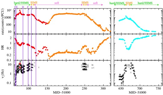
Light curve of PCA count rate normalized to 1 PCU unit in the 3–20 keV range (top) and evolution of hardness ratio (HR) of the 6–20 keV count rate to the 3–6 keV count rate (second panel). The first and second parts of the first outburst are coloured in red and orange, while the second outburst is coloured in cyan. The lower panel shows the central frequencies of LF-QPOs in solid symbols, with harmonics/sub-harmonics as open symbols. Type-C are denoted by black circles, Type-B by dark grey triangles and Type-A and the other unclear structures with light grey crosses. Red stars indicate an irregular type of QPO at which the count rate reached maximum and the strong jet was observed.
Although several authors have already reported the QPO frequencies (e.g. Sobczak et al. 2000; Remillard et al. 2002; Rodriguez et al. 2004), we re-estimated the frequencies using binned mode data to systematically examine their behaviour. The centroid frequencies were determined by fitting the power spectral densities (PSDs) with Lorentzians and/or Gaussians. The calculated frequencies were found to be consistent with the previous results. The LF-QPOs are detected in the SIMS, HIMS, and brighter hard state in both rising and decaying phases (HR ≥ 0.5 and count rates exceeding 100–200 cts · s−1 · PCU−1).
Fig. 2a shows the hardness-intensity diagram (HID) of these outbursts. Data points showing LF-QPOs are identified by different (boldface) symbols, as in the bottom panel in Fig. 1, whereas observations without QPOs are marked by small dots. We select observations corresponding to characteristic points on this diagram, marked A-F. These are also shown on the time history (Fig. 1) for reference, and identified in Table 1.
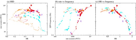
Data from Fig. 1 plotted as (a) Hardness-Intensity, (b) Intensity-QPO centroid frequency and (c) Hardness-QPO centroid frequency, also includes the locations of the selected observations A–F which characterize the source behaviour in different spectral states and/or different luminosity. Colours indicating the outburst time are the same as in Fig. 1, as are symbols indicating the QPO types. In panel (a), the data points without QPO features are shown as small dots, whereas in (b) and (c) the dots are larger so the points can be seen.
Observational data for sample spectra. QPO types were referred from Remillard et al. (2002).
| ID | ObsID | Observation start date | MJD | PCA exposure | Rate | Spectral state | QPO type* |
|---|---|---|---|---|---|---|---|
| (s) | (counts · s−1 · PCU−1) | ||||||
| A | 30191-01-38-00 | 1998/11/01 23:56:32 | 51118 | 3456 | 746.6 | soft | – |
| B | 30191-01-32-00 | 1998/10/20 22:52:48 | 51106 | 880 | 3064.3 | SIMS | B |
| C | 30191-01-28-02 | 1998/10/12 06:33:20 | 51098 | 1632 | 2305.5 | HIMS3 | C |
| D | 30191-01-14-00 | 1998/09/28 08:12:48 | 51084 | 4704 | 2644.9 | HIMS2 | C |
| E | 30188-06-01-02 | 1998/09/10 01:37:20 | 51066 | 3424 | 1885.9 | HIMS1 | C |
| F | 30188-06-03-00 | 1998/09/08 00:09:52 | 51064 | 5664 | 873.7 | hard | C |
Figs 2b and c show the central frequency of the fundamental LF-QPO, νc, plotted against the PCA count rate and HR, respectively. It is clearly evident from Fig. 2b that there are ’parallel tracks’, with the same LF-QPO frequency seen at very different mass accretion rates (i.e. intensity). Typically the LF-QPOs are seen at higher flux in the fast rise than in the slow decay, and at a different flux level for the fast rise in each outburst. However, these separate tracks merge together when the LF-QPO frequency is plotted instead against HR (Fig. 2c). This shows that the spectral shape (i.e. disc-corona geometry) is more important than overall luminosity in determining νc.
3 CONSTRUCTION OF THE SSSED MODEL
3.1 Model description
3.1.1 Concept of the model
As introduced in Section 1, the soft spectral component is generally considered as being produced by the optically thick standard disc, which extends close to the ISCO in the soft state but is truncated far from the ISCO in the hard state. The Comptonization component requires an electron population which is pre-dominantly thermal in the hard state, while non-thermal electrons are evident in the soft state. This change in accretion flow properties makes it difficult to fit the entire outburst with a single model, and transition spectra are especially complicated as they probably require all components so are very difficult to decompose uniquely.
We build on the model used to constrain similarly complex AGN spectra. The data are often fit with radially stratified models, where an outer blackbody emitting standard disc transitions to a Comptonized disc, where the optically thick material does not quite thermalize but instead is Comptonized in warm plasma to form the soft X-ray excess. The disc truncates in the inner regions, with the flow forming a hot, optically thin plasma close to the black hole (the agnsed model in xspec: Kubota & Done 2018). This model is (generally) able to uniquely fit to the complex data even with the absorption gap in the EUV because the components are energetically constrained by the disc emissivity assuming the mass accretion rate is constant with radius.
We tailor this approach to be more tuned to BHBs, and especially to their intermediate spectra where there are clearly two Compton components as well as a (truncated) disc. The key concept is that the flow is radially stratified such that the accretion power is emitted as (colour-corrected) blackbody radiation at r > rcor, while it is emitted as inverse-Comptonization by both the thermal and non-thermal corona at r < rcor. All the emission is constrained by the standard disc emissivity by Shakura & Sunyaev (1973), with |$\dot{M}$| constant with radius. Past work has clearly shown that we can use the temperature and luminosity of the disc component in the high/soft state to determine the mass accretion rate and inner radius of the disc. Here, we will use the same idea to derive the geometry of the more complex states, using the shape and luminosity of the low-temperature soft component to derive the mass accretion rate through the unComptonized disc and its inner radius in the SIMS, HIMS and hard states, with the remaining radial emissivity used to power the Comptonized emission.
3.1.2 Assumed geometries and emissivity
The agnsed model has a truncated outer blackbody disc which is not colour temperature corrected as this was assumed to be subsumed into the warm Comptonization region. The higher temperatures of BHB mean that this is not appropriate so we explicitly include the expected colour temperature correction to the blackbody disc emission as citeoptxagnf. This has assumed angle dependence ∝cos i.
The Comptonizing coronal regions of rin ≤ r ≤ rcor are less well defined. They can have seed photons from a passive disc below the corona which reprocesses the illuminating flux (e.g. Petrucci et al. 2013), or from external direct illumination from the outer disc, or the soft Compton region. External seed photons (from outside rather than from passive disc reprocessing) will add to the emitted luminosity at that radius, making the emissivity at a given radius not exactly defined. The angular radiation pattern is also not well defined. If the Comptonization region is radially extended over the passive disc then it might be ∝cos i or a larger-scale height flow might be more isotropic.
We want to make a model that can be used across all the data, yet both seed photon source(s) and geometry are probably changing with spectral state. After some experimentation, we make a pragmatic choice to fix the seed photon source as reprocessing from a passive disc underneath the Comptonizing coronae, and to assume these emit isotropically. Then the local luminosity at radius r Fcor(r) = Lcor(r)/(4πd2), while the observed flux from the outer disc (r > rcor) is represented as Fdisc(r) = Ldisccos i/(2πd2). This geometry of the code is shown in Fig. 3, but we stress that assumption of an underlying passive disc is so as to easily determine a seed photon energy for the model.
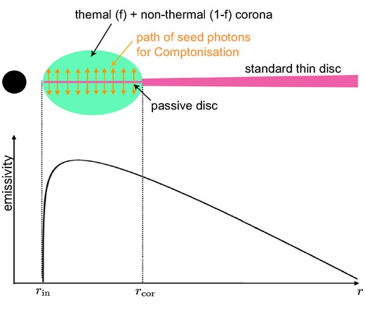
Sketch of model geometry and radial emissivity profile.
We neglect irradiation of the outer disc by the Comptonization regions as this has negligible effects on the X-ray spectra of BHBs in the luminous disc states. Reprocessing can affect the disc emission in the hard state because the intrinsic disc luminosity is small compared to the irradiating Compton luminosity. However, the disc temperature is also low so it is difficult to tightly constrain from RXTE data in this state. We also neglect general relativistic ray tracing as we assume these are subsumed into the inclination/geometry uncertainties detailed above.
The mass accretion rate |$\dot{M}$| is assumed to be constant throughout the accretion flow from rin to rout, but the efficiency is now defined as in Newtonian gravity as η = 0.5 · (rin/rg)−1. Since rin may now change, we normalise the mass accretion rate to the Eddington accretion rate defined without including efficiency, so |$\dot{m}\equiv \dot{M}/\dot{M}_{\rm Edd}$|, where |$\dot{M}_{\rm Edd}$| is defined as |$\dot{M}_{\rm Edd}c^2=L_{\rm Edd}$|. A changing inner radius could be a real aspect of a large-scale height flow, either from magnetic connection allowing it to tap the gravitational potential inwards of the ISCO, or Lense-Thirring torques which truncate the flow above the ISCO. Alternatively it could just be a small compensation for some of the geometry uncertainties (inclination dependence and relativistic ray tracing) noted above. We term this model SSsed (meaning Shakura–Sunyaev SED), with emissivity |$\epsilon (r)=3GM \dot{M} f(r)/(8\pi r^3)$| where |$f(r)=(1-\sqrt{r_{\rm in}/r})$|.
Details of spectral parameters of the SSsed model are shown in Appendix A.
3.1.3 Regions of comptonizing components
It is very clear from the data that there is thermal Comptonization in the hard state, and non-thermal in the soft state. However, many good-quality spectra extending over a broad bandpass require that there are two Compton components, e.g. Yamada et al. (2013) and Basak et al. (2017) for Cyg X-1, Zdziarski et al. (2021) for MAXI J1820 + 070, and Kubota & Done (2004) and Hjalmarsdotter, Axelsson & Done (2016), Connors et al. (2019) for XTE J1550 − 564.
To allow the model to fit across all spectral states, we allow the energy to be released through hot thermal and/or non-thermal inverse Compton scattering within rcor. We assume the same emissivity as for the standard disc region. This would not be appropriate for the advection-dominated accretion flow (ADAF; Narayan et al. 1998) in faint states with |$\dot{m} \le 0.1$|, where the emissivity is significantly lower than that of the standard disc. However, in this paper, we focus on the luminous X-ray states where |$\dot{m}$| is larger than 0.1.
We used the nthcomp model (Zdziarski, Johnson & Magdziarz 1996; Życki, Done & Smith 1999) to model the Comptonized emission as in agnsed model. The nthcomp model describes thermal Comptonization parametrized by photon index Γ and electron temperature kTe. However, we also use this model to describe the effect of non-thermal Comptonization from a steep power-law electron distribution. A power-law electron distribution produces a power law from inverse Compton scattering, similarly to a Maxwellian (thermal) distribution. The major difference is that thermal electrons produce a cutoff in the spectrum at ∼3kTe, which is not present in the non-thermal case. Instead, a steep electron distribution has a spectral break at 511 keV from the Klein–Nishima cross-section (see e.g. Hjalmarsdotter, Axelsson & Done 2016). This can be well approximated by thermal Comptonization with kTe = 300 keV in data which do not extend beyond ∼150–200 keV, so we use the nthcomp model for this case also. Therefore, in this paper, the term ‘non-thermal’ is employed to signify the absence of a discernible cut-off within the observed energy band. We allow there to be both thermal and ‘non-thermal’ electrons in the same region, parametrized by the fraction of accretion power, fth, in the thermal Compton, and |$\dot{m}_{\rm non}=(1-f_{\rm th})\dot{m}$| in non-thermal Comptonization.
We assume the seed photons come from a passive disc underneath the Comptonization region. In this case, all the accretion power is supplied to the corona, while the disc itself is originally completely dark. The corona irradiates the disc, which reprocesses the radiation into a blackbody which is as hot as the original standard disc (see e.g. Kubota & Done 2018). Therefore, the seed photon temperature for the local Comptonization is set to be the colour-corrected passive disc temperature at radius r. We calculate the released accretion power for a given |$\dot{m}$| at radius r, and normalize nthcomp emission to suit for the predicted local luminosity at r. This is the same method employed for the disc-corona region in agnsed model. We note that the corona intercepts all the photons from the disc, so there is no reflection component from this where the corona is optically thick.
4 ANALYSES AND RESULTS
For spectral analyses, we utilized 3–20 keV spectral data from the PCA and 20–150 keV data from the High-Energy X-ray Timing Experiment (HEXTE). The source and background spectral files and the response matrix files, were obtained from the standard data products provided by the RXTE guest observer facility.2 To take systematic uncertainty on calibrations into account,3 0.5 per cent systematic errors were included to each energy bin.
In addition to the continuum emission modelled by the SSsed model, we included a Gaussian line and smeared edge (smedge) to approximately model the reflection features as well as complex absorption and emission features around ∼6–10 keV. Since the disc is expected to be highly ionized, the shape of the reflected emission is similar to that of the original hard X-ray component, except for the iron structures around 6–20 keV. Therefore, for efficient computation time we opted to use the phenomenological smedge and Gaussian models instead of employing a full reflection code for all the spectral data.
The spectrum is modified by interstellar absorption, modelled using tbabs with the abundance given by Wilms, Allen & McCray (2000), so the total xspec model is described as
where the values of M, NH, d and i are fixed to be 9 M⊙, 9.0 × 1021 cm−2, 4.4 kpc and 75°, respectively. We also fixed the width of smedge at 5 keV. We constrain the edge energy to be 7.2–9.2 keV, central energy Ec and σ of Gaussian to be 6.2–6.9 and 0.1–0.8 keV, respectively, and photon indices of two Comptonizing components in SSsed to be 1.4–4.0. The normalizations between PCA and HEXTE were adjusted by adding constant parameter to the model description, and the presented parameters are based on the PCA normalization.
We examine the effect of reflection in more detail in a series of Appendices. First, we demonstrate that simpler disc plus single Compton and its full reflection cannot fit all the spectra (see Appendix B). We then demonstrate that our SSsed geometry is not significantly changed from including full reflection on both Compton components compared to the much simpler and faster phenomenological approach used here (see Appendix C).
4.1 Example spectral fits to each state
We first demonstrate that the model can fit all the separate spectral states seen during the outburst, and that the key parameters that are rcor and |$\dot{m}$|, are not much changed by more detailed reflection modelling.
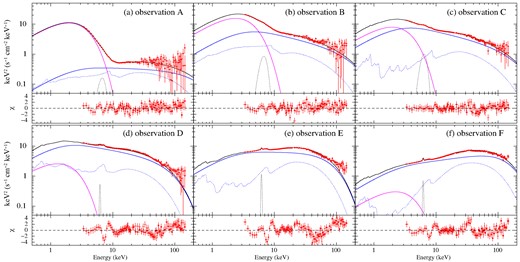
Figs 4a–f show the spectra of observations A–F (identified in Fig. 2a) with the best-fitting SSsed model, with parameters shown in Table 2. The model components are colour-coded with magenta for the outer standard disc, blue for the non-thermal steep Compton component, and green for thermal Compton component. Considering the HR values and count rate, as well as the PSDs (shown in Fig. D1 in Appendix D), the spectral states of observations A, B, C, D, E, and F are consistent with the soft state, SIMS, (softer)HIMS, HIMS, (harder)HIMS and bright hard state [as in previous spectral analyses e.g. Kubota & Makishima (2004), Kubota & Done (2004)].
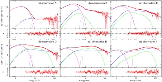
Unabsorbed, deconvolved spectra of observations A–F with the best-fitting SSsed model and residuals between the data and models. Model component of the thermal and non-thermal Comptonizing corona regions are shown in green and blue, respectively, and that of the outer standard disc is in magenta. In observation F, the higher and lower temperature thermal Comptonizing components are shown in blue and green, respectively.
The best-fitting parameters of SSsed model for observations A–F. The values of M, NH, d, and i are fixed to be 9 M⊙, 9.0 × 1021 cm−2, 4.4 kpc and 75°, respectively. The width of the smedge is fixed to be 5 keV. †Values in the parentheses are fixed. *Parameters hit the lower or upper limit.
| Obs. | A | B | C | D | E | F |
|---|---|---|---|---|---|---|
| state | soft | SIMS | HIMS3 | HIMS2 | HIMS1 | hard |
| parameters of the SSsed | ||||||
| |$\log \dot{m}$| | |$0.167^{+0.021}_{-0.019}$| | |$0.38^{+0.05}_{-0.04}$| | |$0.262^{+0.005}_{-0.006}$| | |$0.260^{+0.006}_{-0.005}$| | 0.115 ± 0.009 | |$-0.038^{+0.007}_{-0.006}$| |
| rin(rg) | |$5.46^{+0.18}_{-0.15}$| | |$4.4^{+0.4}_{-0.3}$| | (4.5)† | (4.5)† | (4.5)† | (4.5)† |
| rcor(rg) | |$7.52^{+0.22}_{-0.20}$| | |$9.6^{+1.1}_{-0.9}$| | 11.9 ± 0.3 | |$15.1^{+0.4}_{-0.6}$| | |$25.4^{+1.3}_{-1.1}$| | |$28.6^{+1.1}_{-0.9}$| |
| Γnth | 2.02 ± 0.03 | |$2.34^{+0.03}_{-0.05}$| | |$2.26^{+0.09}_{-0.10}$| | |$2.22^{+0.11}_{-0.16}$| | |$1.99^{+0.06}_{-0.08}$| | 1.679 ± 0.013 |
| kTe(keV) | (300)† | (300)† | (300)† | (300)† | (300)† | |$46^{+10}_{-5}$| |
| fth | (0)† | 0.16 ± 0.06 | 0.28 ± 0.13 | 0.52 ± 0.16 | 0.48 ± 0.09 | |$0.22^{+0.03}_{-0.02}$| |
| Γth | — | |$4.0^{+0.0*}_{-0.9}$| | |$2.23^{+0.08}_{-0.18}$| | |$2.08^{+0.07}_{-0.14}$| | |$1.70^{+0.07}_{-0.08}$| | |$1.40^{+0.05}_{-0.00}$| |
| kTe(keV) | — | (9.0)† | (9.0)† | 8.6 ± 1.0 | |$8.7^{+0.5}_{-0.6}$| | |$10.2^{+0.5}_{-0.4}$| |
| Parameters of smedge and Gaussian | ||||||
| Eedge(keV) | |$9.01^{+0.19*}_{-0.17}$| | |$8.9^{+0.3}_{-0.4}$| | |$8.3^{+0.4}_{-0.2}$| | |$7.82^{+0.26}_{-0.18}$| | |$7.76^{+0.21}_{-0.18}$| | |$7.57^{+0.14}_{-0.12}$| |
| τmax | |$0.89^{+0.11*}_{-0.13}$| | |$0.56^{+0.11}_{-0.09}$| | |$0.52^{+0.10}_{-0.11}$| | |$0.47^{+0.08}_{-0.13}$| | |$0.34^{+0.06}_{-0.10}$| | 0.42 ± 0.04 |
| Ec(keV) | 6.5 ± 0.17 | |$6.36^{+0.20}_{-0.11}$| | |$6.20^{+0.06}_{-0.00*}$| | |$6.27^{+0.09}_{-0.07}$| | 6.34 ± 0.08 | 6.31 ± 0.11 |
| σ(keV) | |$0.80^{+0.00*}_{-0.07}$| | |$0.77^{+0.03}_{-0.39}$| | |$0.66^{+0.14}_{-0.22}$| | |$0.51^{+0.25}_{-0.22}$| | |$0.50^{+0.18}_{-0.17}$| | |$0.18^{+0.24}_{-0.08}$| |
| norm (× 10−3) | |$7.13^{+1.3}_{-1.2}$| | |$36^{+9}_{-18}$| | |$37 ^{+17}_{-14}$| | |$36^{+23}_{-12}$| | |$24^{+9}_{-6}$| | |$4.7^{+1.5}_{-1.1}$| |
| EW(eV) | |$190^{+33}_{-32}$| | |$132^{+33}_{-67}$| | |$165 ^{+72}_{-61}$| | |$135^{+89}_{-43}$| | |$129^{+46}_{-30}$| | |$56^{+19}_{-12}$| |
| χ2(dof) | 109.3(116) | 119.2(114) | 90.3(115) | 89.2(114) | 113.6(114) | 131.7(113) |
Following the typical spectral studies of the soft state spectra, the fitting of the soft state data did not include the thermal Comptonizing component (Fig. 4a). In the SIMS (Fig. 4b), it generally also requires a very steep power-law like component (Γ = 2.5–4, with an upper limit of 4) together with the non-thermal Comptonizing corona (kTe = 300 keV and Γ ≥ 2). The HIMS (Figs 4c–e), most clearly need a combination of thermal and non-thermal Comptonization to fit the data. The bright hard state (Fig. 4f), is difficult to fit with the thermal and ‘non-thermal’ approach due to the shape of the cutoff. However, this can work with similar luminosities derived for the total Comptonized emission with more detailed reflection modelling (Appendix C). This does not change the derived radii and luminosity significantly (see Appendix C).
We now discuss in more detail the fits to each state.
4.2 The soft state and SIMS: inner radius
In order to evaluate rin, the SSsed model was first applied to the spectra in the soft state. As exemplified by observation A shown in Table 2 and Fig. 4a, all the data in the soft state were well reproduced with the model of a disc and a single non-thermal steep Comptonization (so we fix fth = 0) except for one anomalous spectrum on MJD 51262 (ObsID 40401-01-64-00).
In the soft state, the value of rin were found to be almost constant at (5–5.5)rg, which corresponds to spin parameter of a* = 0.15, by considering rin = risco. When the sample spectra of observation A (the typical soft state) was fit by replacing SSsed to kerrbb (Li et al. 2005)4 plus nthcomp, the spin parameter was estimated to be a* = 0.15 ± 0.01 with |$\dot{m}=4.37\pm 0.07$|, which was exactly same as that obtained by rin in the SSsed model.
We examined the data from the SIMS. We allow both thermal and non-thermal Comptonization, though the thermal Comptonization is not always required. Fig. 4b illustrates the SIMS spectrum (observation B), where the weaker and steeper (Γth = 4) Comptonization (green) is seen between the outer disc (magenta) and the flatter non-thermal corona (blue). As seen in this figure, the additional steep component is much weaker and steeper than the flatter Comptonizing component, and thus it was not able to be distinguished whether it is thermal (with a cut-off) or non-thermal (without a cut-off). Instead, we fixed kTe at 9 keV, which is an average value of the thermal Comptonization component in the HIMS (see Section 4.3). It is important to note that the uncertainty of kTe does not affect the fitting result.
In the SIMS, the values of rin were found to be ∼4.5rg on average. Details of rin in the SIMS are presented in Appendix E. The value of 4.5rg is slightly smaller than rin of (5.0–5.5)rg in the soft state, and the difference is statistically significant, since |$\chi ^2_\nu$| values become much worse if spectra in the SIMS were fit with the SSsed by fixing rin at 5.5rg. This could be a real effect, where the non-thermal region is given additional emissivity from magnetic connection across the ISCO, but it seems more likely that it arises from the model uncertainties and approximations (e.g. slight difference from isotropic geometry in the corona region, geometry changes coupled with relativistic effects, or slight difference of inclination angle). Consequently, we refer the average value of 4.5rg as an apparent reference value for constant rin (i.e. similar to risco) in the SIMS. This difference, which is up to 20 per cent, could be the systematic uncertainty to estimate absolute values of corona radius rcor.
4.3 The HIMS
The HIMS spectra required the inclusion of both thermal and non-thermal Comptonization components. The examples of spectral fits of HIMS data are shown in Fig. 4c–e. Fig. 5 presents the evolution of the spectral parameters in the HIMS and hard state.
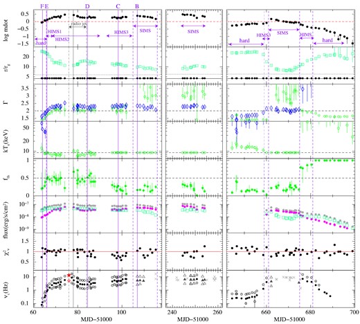
Time evolution of the best-fit parameters of the SSsed. Parameters shown are (first panel) |$\log \dot{m}$|, with a horizontal dashed lines indicating |$\dot{m}=1$|. (Second panel) The corona radii rcor (open square) and rin (black dots, fixed at 4.5rg). The rcor values can be compared with the effective radius rmax(= (7/6)2rin = 1.36rin) shown with the dotted line. At rmax, the local emissivity |$\sigma T_{\rm eff}^4$| becomes maximum in the framework of the Shakura–Sunyaev standard disc. (Third panel) the photon index of the non-thermal (Γnth, blue diamonds) and thermal (Γth, green circles). (Fourth panel) Electron temperature of thermal Comptonizing corona. (Fifth panel) The fraction of thermal Comptonizing corona, fth. (Sixth panel) Bolometric flux values of the disc (filled magenta circles), Comptonizing corona (open squares) and total (filled grey circles). (Seventh panel) Reduced chi-squared values |$\chi ^2_\nu$|, with horizontal solid line indicates |$\chi ^2_\nu$| of 1, (Eigth panel) QPO frequencies repeated from Fig. 1. Vertical solid lines indicate the locations of observations B–F, and the vertical dashed lines distinguish the spectral states, and vertical dash–dotted lines indicate the times at which the strong radio jet was detected, with maximum on MJD 51077–51078 (Hannikainen et al. 2009) as solid grey line.
The outer radius of the disc-corona region, rcor, was observed to be much larger than that in the soft state and SIMS. As a result, and the temperature of outer thin disc, T(rcor), is too low to be constrained in the energy range of the PCA, despite the high luminosities. Therefore, throughout the spectral fit, the values of rin were fixed to be an average value of rin in the SIMS, 4.5rg (see Section 4.2). Moreover, to achieve satisfactory |$\chi ^2_\nu$| values, the hot Comptonizing component with thermal cut off (represented by the green lines in Figs 4c–e) is always necessary, and fth, Γth, and kTe were treated as a free parameter. In this figure, the same SIMS data were analysed in the same manner as described in Section 4.2, but with a fixed value of rin at 4.5rg. This was done to facilitate a comparison of the results with those obtained in the HIMS and hard state, without considering uncertainties.
As seen in the second bottom panels of Fig. 5, almost all the data points in the HIMS were successfully reproduced with the SSsed, except for the data obtained around a strong radio jet event on MJD 51076–510775 (Hannikainen et al. 2009). These data probably indicate that there are additional processes from the jet, which are not included in the baseline SSsed model. We thus exclude these data from our discussion based on the SSsed model.
During the first outburst in the HIMS phase, the size of the corona region, rcor, was ∼25rg(= 6rin) at the onset (MJD 51066), decreasing to ∼16rg(∼ 4rin) on MJD 51068. Except for the radio jet duration, it underwent a change to approximately (11–15)rg by MJD 51087, gradually decreasing to (11–13)rg during the softer HIMS phase (MJD 51095–51101), and eventually reaching (8−10)rg in the SIMS phase (MJD 51106–51115). From MJD 51066 to 51087, the contributions of thermal and non-thermal Comptonization were almost equal, with fth ranging from 0.4 to 0.6. However, from MJD 51095 to 51101, shortly before the start of the SIMS phase, the value of fth decreased to 0.1–0.2. Therefore, we categorize the epochs into HIMS1 (MJD 51066–51068), HIMS2 (MJD 51068–51087), and HIMS3 (MJD 51087–51095), ranging from hard to soft. In the second outburst, the HIMS data on MJD 51660 are consistent with those of HIMS3 based on the values of fth and rcor. Additionally, the data on MJD 51675–51680 are likely in the HIMS phase but are difficult to distinguish due to their faintness.
During the HIMS1 phase of the first outburst, the non-thermal Comptonizing component was observed to have a spectral index of Γnth ∼ 2.0, which then evolved to become steeper, reaching values of 2.2 ∼ 2.3. This steeper spectral index was maintained throughout the HIMS2 and HIMS3 phases. Similarly, the thermal Comptonization component showed variations, starting with a harder spectrum characterized by Γ ∼ 1.7 and kTe ∼ 9 keV, and then transitioning to a softer spectrum with Γ = 2–2.2. During the fitting of the HIMS3 data, the weaker thermal component did not allow for a reliable determination of kTe, so it was fixed at an average value of 9 keV. During HIMS1, y-parameter and optical depth τes of thermal Comptonizing corona varied from τes ∼ 7 and y ∼ 3 to τes ∼ 5 and y ∼ 1.
4.4 The hard state: rising and decaying phases
The hard state spectra in the bright rising phase of the outbursts (until MJD51065 in the first outburst and MJD51644–51655 in the second outburst) posed challenges when fitting them using the framework of thermal and non-thermal Comptonization. The reduced chi-squared values were relatively high with hard spectral index of Γnth ∼ 1.7, with |$\chi ^2_\nu$| value of 1.4 with d.o.f. of 114 on MJD51064 (observation F) in the rising phase of the first outburst, and |$\chi ^2_\nu$| values ranging from 1.4 to 1.8 with d.o.f. of 108 on MJD51644–51655 in the second outburst. There is no clear evidence of a disc in these spectra, so we again fix rin to 4.5rg as seen in the SIMS (see Section 4.2).
There was no clear evidence of a non-thermal power-law-like Comptonizing component in these spectra. Instead, the dominant spectral component appeared to be hot thermal Comptonization with a relatively hard photon index (Γ < 2). However, these spectra could not be adequately reproduced using a single Comptonization model (see details in Appendix B). Previous studies of the bright hard state by Kawamura et al. (2022, 2023) have suggested the presence of multitemperature Comptonization to explain similar complex spectral features, and Yamada et al. (2013) also suggested the two-temperature Comptonization for Cyg X-1 in the hard state.
Therefore, we attempted to fit these spectra with the same SSsed model but allowing the temperature (kTe) of both Comptonizing components to vary freely. As a result, the spectra were successfully reproduced by employing two thermal Comptonization components: one with a higher temperature (kTe = 40–70 keV) and a photon index of Γ = 1.6–1.8 (i.e. τes = 3–2, y = 3–2), and the other with a lower temperature (kTe ∼ 10 keV) and a photon index of Γ = 1.4–1.6 (i.e. very large τes = 9–7 and y = 7–4). Fig. 4f shows an extreme case of this spectral fit taken from observation F. While the presence of two thermal Comptonization components in the spectra of the bright hard state during the rising phase of the outbursts provides insight into the evolution of non-thermal Comptonization, investigating the detailed structure of the hard state is beyond the scope of this paper. Instead, we utilised the estimated values of rcor obtained from the improved spectral fits as a result of this analysis.
During the decaying phase of the outburst, the spectra in the low/hard state were successfully reproduced using a single hot thermal Comptonization component. As the system transitioned from the HIMS to the hard state (between MJD 51680 and 51682), the spectral characteristics changed, with a dominant hot Comptonizing component and no significant contribution from a steep non-thermal hard X-ray component originating from the disc-corona region. The spectra were well described by a single hot Comptonization component with a photon index of Γ = 1.6–1.7 and electron temperature of kTe ≥ 50 keV. The coronal radii were found to extend further as 20rg to 30rg. However, during this phase, the accretion rate (|$\log \dot{m}$|) was determined to be less than −0.5, corresponding to only 3 per cent of the Eddington luminosity. As a result, it is expected that the ADAF (Narayan et al. 1998) is realized instead of the assumed Shakura–Sunyaev emissivity.
4.5 Summary of model parameters from the fits
Fig. 5 shows how the derived parameters of the SSsed change across the outburst. There is a very nice smooth variation in rcor with time despite the large changes in spectral shape, with Comptonization changing between thermal and non-thermal. The fits are generally very good (the very poor fits around a strong radio jet event on MJD 51076–51077 noted above are excluded from the analysis).
5 DISCUSSION
5.1 Anticorrelation between the corona size and LF-QPOs
We now explore how the QPO depends on the SSsed model parameters. Fig. 6 shows the QPO frequency versus the overall mass accretion rate, |$\log \dot{m}$|. This shows the same parallel track behaviour as in Fig. 2b as the derived |$\dot{m}$| is closely linked to the observed intensity. Instead, it is clear that the QPO frequency depends more tightly on the spectral shape (Fig. 2c), which is determined mainly by rcor in the SSsed model.

QPO centroid frequency, νc, versus |$\log \dot{m}$|. Clearly there is the same ‘parallel tracks’ behaviour as in Fig. 2 b of QPO centroid versus intensity, as |$\dot{m}$| is closely related to intensity. The locations of observations B–F are indicated with open squares. Values of rin in the hard state, HIMS, and SIMS are fixed at 4.5rg, and the soft state data (without fixing rin) are identified with grey open circles. Type-C and Type-B QPOs are identified with circles and triangles, respectively, while Type-A QPOs and the other unclear structures are identified with crosses. Colour-coded according to observation dates of MJD − 51000.
Fig. 7a presents the QPO centroid frequency plotted against the estimated rcor. This figure clearly illustrates the strong anticorrelation between νc and rcor throughout all phases of the outburst. In order to account for potential systematic uncertainties in determining rcor during the hard state, the data points corresponding to the hard state are displayed with fainter colours. It is important to note that the low/hard state with |$\log \dot{m}\lt -0.5$| likely exhibits the influence of an ADAF, which is not accounted for in the SSsed model. Similarly, the bright/hard state displays a complex corona structure (see Section 4.4). Additionally, in the hard state, the reverberation signal suggests a strong enhancement of outer disc emission due to reprocessing caused by irradiation from Comptonizing emission. Such reprocessing effects are not included in the SSsed model, which may lead to inaccuracies.
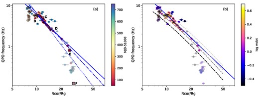
QPO centroid frequency, νc, versus outer radius of Comptonizing region, rcor/rg. Values of rin in the hard state, HIMS, and SIMS are fixed at 4.5rg, and the soft state data (without fixing rin) are identified with grey open circles. The data points from the hard state shown in fainter colour. QPO types are identified with the same symbols in Fig. 6. (a) Colour-coded according to observation dates of MJD − 51000. Blue lines represent the best-fitting power-law. The blue dotted line (all the data), solid line (without the hard state data), and dash-dotted line (the HIMS data alone) represent |$\nu _{\rm c}=2359\cdot r_{\rm cor}^{-2.559}$|, |$\nu _{\rm c}=434\cdot r_{\rm c}^{-1.865}$|, and |$\nu _{\rm c}=874\cdot r_{\rm cor}^{-2.126}$|, respectively. (b) Colour-coded according to |$\log \dot{m}$|. Overlaid are the relations between LT precession frequency and the outer radius of a hot flow (taken from Fig. 5 in IDF09) for spins of a* = 0.3 (black), 0.5 (dark grey), 0.7 (light grey), and 0.998 (lighter grey), shifted up by a factor of 1.11(= 10 M⊙/9 M⊙).
By excluding the data points from the hard state, we find that the anticorrelation between rcor and νc can be approximated by power-law relationship: νc = 434 · (rcor/rg)−1.865 Hz. Similarly, the relation ship of νc = 874 · (rcor/rg)−2.126 was obtained by the HIMS data alone.6 Indeed, the observed anticorrelation between νc and rcor provides an empirical description of the relationship between QPO centroid frequency and the extent of the hard X-ray corona. This relationship holds consistently across different outbursts, as represented by the variation in colour, as well as different types of QPOs, as represented by the different symbols used in the plot. This suggests a robust connection between the QPO properties and the characteristics of the corona, emphasizing the significance of the corona in driving the QPO behaviour.
This conclusion is consistent with a previous study by Marcel et al. (2020) which also found that the frequency of QPOs is related to the energy-conservation of an inner jet-emitting disc (Ferreira et al. 2006; Marcel et al. 2019) and an outer standard disc, based on radio, X-ray, and γ-ray observations.
5.2 Comparison between the observation and the LT prediction
In order to compare the observed anticorrelation between νc and rcor with theoretical predictions proposed to explain the LF-QPOs, we focus on investigating the relativistic Lense–Thirring precession scenario in this paper.
The relativistic LT precession was first proposed as a candidate to cause LF-QPOs by Stella & Vietri (1998), and it has been extensively studied since by many authors including IDF09 and Motta et al. (2014). IDF09 coupled the mechanism with the truncated disc/hot inner flow geometry to predict an anticorrelation between νc and the inner radius of the truncated disc (which corresponds to the outer radius of geometrically thick hot inner flow). Fig. 7 b shows the same νc-rcor plot as in Fig. 7 a but colour coded by |$\log \dot{m}$|.
In Fig. 7b, the predicted νc-rcor relations based on LT precession scenario by IDF09 are overlaid with dashed lines for spin parameters of a* = 0.3, 0.5, 0.7, and 0.998 (lower to upper lines). The predicted lines are taken from Fig. 5 in IDF09 (though we note that these are for a fiducial mass of 10 M⊙ rather than the 9 M⊙ used here). The observed νc–rcor relations are consistent with the LT prediction. This result is strongly supporting LT precession as a probable candidate for the origin of the LF-QPOs. However, there is still some scatter in the data points around the predicted lines. They do not exactly pick out a single spin parameter track in the LT models, though they are supposed to concentrate on the lines a* = 0.5–0.7.
This is not surprising given the LT model simplicity in IDF09, where the precessing Comptonized region is assumed to have fixed scale height for all |$\dot{m}$|. It seems more likely that the Comptonization geometry is changing during the state transition, so that the scale height decreases as the Compton cooling becomes larger. This changes the predicted LT precession frequency, as well as changing the spectra (by changing the inclination dependence and relativistic corrections) in a way which is not included in SSsed. Moreover, the SSsed model also does not include the jet power, yet there is a steady compact jet in the bright hard state and HIMS spectra which is powered by the accretion flow (e.g. Fender, Belloni & Gallo 2005), and there are discrete blobs ejected at the HIMS/SIMS transition (e.g. Wood et al. 2021).
Perhaps a more serious issue is that the disc-dominated spectra in this source give a black hole spin of a* ∼ 0.15 when fit with kerrbb or rin = 5.5rg for the assumed binary parameters of d = 4.4 kpc, i = 75° and M = 9 M⊙ (see section 4.2). This seems very low to cause the strong precession required to produce the large QPO amplitude observed. However, we note that there are uncertainties on these values, and closer distance and higher mass results in larger black hole spin. Including these system uncertainties gives a wider range of spin estimates from the disc-dominated spectra, of 0.1 < a* < 0.7 (Davis, Done & Blaes 2006) or −0.11 < a* < 0.76 (Steiner et al. 2011) with Connors et al. (2020) using the spin of ∼0.5 to encompass all current estimates.
Finally, it is important to note that while the role of LT precession has been primarily proposed to explain Type-C QPOs, there is no significant observational difference in the behavior of Type-B (and A) QPOs in the νc–rcor relation in view of the frequencies. Our analysis indicates that both types of QPOs are consistent with the LT precession scenario, with Type-B (and A) QPOs appearing at the high νc and small rcor end of the νc–rcor relation, although there may be some scatterings.
5.3 Issues for LT precession models
To construct the SSsed model, we utilized the passive disc scenario to provide seed photons to the Comptonizing component. It should be noted that LT precession, being a vertical precession, so is challenging to occur if there are obstacles present in the mid-plane. However, in the calculations of the SSsed model, the passive disc primarily serves as a source of seed photons for the coronae. The specific details of the seed photon structure have minimal impact on the overall results. Hence, slight variations or changes in the seed photon structure do not significantly influence the obtained results in the model. The presence of strong non-thermal Comptonization in the HIMS and SIMS indicates the need for a substantial source of seed photons, which can be from strong external irradiation from the truncated disc and/or the steep Comptonization can provide seed photons for the thermal Comptonization. Alternatively, the passive disc can have a clumpy structure, so that the hot plasma can precess through the mid-plane holes. Such a clumpy structure may be consistent with optically thick blobs predicted in GRMHD simulations (Liska et al. 2022).
In fact, there was no significant difference in estimating the size of the outer corona, rcor, when we changed slightly the corona geometry. For example, we tried to fit the data with truncated disc-(non-thermal) corona and inner hot flow geometry, the obtained νc–rcor relation are almost the same and still consistent with the LT prediction. Therefore, we can conclude that the estimation of rcor is quite robust, as it is primarily determined by the combination of the outer disc’s shape and luminosity, as well as the relative luminosity of the outer disc compared to the Comptonization components.
In addition, LT precession of the entire Comptonized flow matches (to zeroth order) all the QPO types seen here, not just the Type-C QPOs, with Type-B and Type-A QPOs appearing at the smallest rcor values in these data rather than being offset as might be the case if these were really from a different mechanism/geometry (see e.g. the review by Ingram & Motta 2019).
Totally, the observed νc–|${\rm r_{\rm cor}}$| relation is consistent with its theoretical prediction calculated by IDF09. However, it is important to note that the scenario of LT precession as the origin of LF-QPOs is still being questioned by some authors. For example, Marcel & Neilsen (2021) demonstrated that the accretion flow can reach sonic or supersonic speeds in the bright hard state, which prevents the ‘wave-like’ regime required for solid-body precession to cause LF-QPOs. This can also result in strong changes in the predicted QPO frequency due to the magnetic interaction of the precessing flow with the outer disc (Bollimpalli, Fragile & Kluźniak 2023).
Therefore, further theoretical studies including GRMHD simulations are necessary to understand the LF-QPO behaviour. Nevertheless, the observed νc–rcor relation can provide a useful guideline to investigate the validity of theoretical models for LF-QPOs.
6 SUMMARY AND CONCLUSION
We developed the spectral model SSsed by modifying the multicomponent AGN model agnsed to tailor it for stellar BHBs. We applied it to the X-ray spectra of XTE J1550 − 564 observed with RXTE to determine the size of Comptonizing corona in different states. Except for the data obtained around a strong radio jet event on MJD 51076–51077 and during the rising phase of outburst, the SSsed model successfully reproduced the spectra of XTE J1550 − 564.
In the HIMS, both thermal (kTe = 8–20 keV) and non-thermal (Γ = 2–2.4 without clear cut-off energy) corona were required to reproduce the Comptonizing component. The outer corona radii were found to vary from 10rg to 25rg. In the SIMS, though the hard emission was dominated by the non-thermal Comptonizing component, an additional steeper (Γ ≤ 2.5) Comptonizing components improved the spectral fits with fraction of fth = 0.1–0.3. The corona radii were found at (8–10)rg.
The hard state spectra did not require the non-thermal Comptonizing component. On one hand, in the hard state during the decaying phase of the second outburst, the spectra were well represented by a single hot Comptonizing component with Γ = 1.6–1.8 and kTe ∼ 50 keV at rcor > 20rg. On the other hand, spectra in the bright hard state during the rising phase of the outbursts were difficult to be fit within the framework of thermal and non-thermal Comptonizing corona. Instead, the spectra were reproduced with a two-temperature thermal Comptonizing corona, which is consistent with the findings suggested by Kawamura et al. (2022), Kawamura et al. (2023).
By comparing the obtained corona outer radii rcor to the centroid LF-QPO frequency, νc, we found a tight anticorrelation between νc and rcor, described approximately as |$\nu _{\rm c}=434\cdot r_{\rm c}^{-1.87}$| (without the hard state data) or |$874\cdot r_{\rm cor}^{-2.13}$| (with the HIMS data alone). This relation is in remarkably good qualitative and quantitative agreement with the prediction of LT precession (IDF09). We conclude that the intermediate states, which show both strong disc emission and strong LF-QPOs, provide the best data to test QPO formation models despite the complexity of these spectra.
ACKNOWLEDGEMENTS
AK thanks S. Mineshige and T. Kawashima for their helpful discussions. AK acknowledges the support received from the discretionary fund of the President of Shibaura Institute of Technology. CD acknowledges the Science and Technology Facilities Council (STFC) through grant ST/T000244/1 for support, and University of Tokyo Kavli IPMU. We also thank R. Connors for his detailed reading as a reviewer.
DATA AVAILABILITY
The RXTE data underlying this article are available in NASA’s HEASARC archive site at https://heasarc.gsfc.nasa.gov/docs/archive.html.
Footnotes
kerrbb was used under the condition of zero torque at the inner boundary, without limb-darkening and self-irradiation, and with a hardening factor of 1.7 (Shimura & Takahara 1995).
The fits were not improved even if the the value of Γth was not constrained.
Power-laws of νc = 2359 · (rcor/rg)−2.559 Hz was obtained with all the data including the hard state.
References
APPENDIX A: SPECTRAL PARAMETERS OF THE sssed MODEL
Spectral parameters of the SSsed model are summarized in Table A1. The model has some switching parameters. If parameter 6 is negative, the model gives the inner hot Comptonization component. If parameter 7 is negative, the model gives the Comptonization component in the passive-disc corona region. If parameter 9 is negative, the model gives the outer disc. If parameter 12 is −1, the code will use the self-gravity radius as calculated from Laor & Netzer (1989). Colour correction is included when parameter 13 is fixed to be 1, while it is not included when this parameter is fixed to be 0. For BHB spectra, this parameter should be fixed to be 1.
Spectral parameters of the SSsed model.
| Description | |
|---|---|
| par1 | Mass, black hole mass in solar masses |
| par2 | Dist, comoving (proper) distance in kpc |
| par3 | |$\log \dot{m}$|, |$\dot{m}=\dot{M}/\dot{M}_{\rm Edd}$| where |$\dot{M}_{\rm Edd}c^2=L_{\rm Edd}$| |
| par4 | rin, inner most radius of the accretion flow in rg |
| par5 | cos i, inclination angle of the disc |
| par6 | kTe, th, electron temperature for thermal corona in keV. If this parameter is negative, the model gives the inner hot Comptonization component. |
| par7 | kTe, nth, apparent electron temperature for non-thermal corona in keV which is recommended to be fixed at 300 keV to mimic non-thermal electron distribution. If this parameter is negative, the model gives the Comptonization component in the passive-disc corona region. |
| par8 | Γth, photon index of inner hot corona. If this parameter is negative then only the inner Compton component is used. |
| par9 | Γnth, photon index of disc-corona. If this parameter is negative, the model gives the outer disc. |
| par10 | fth, fraction of the hot Comptonizing component to the total Comptonization |
| par11 | rcor, outer radius of the disc-corona region in rg |
| par12 | log rout, outer radius of accretion disc in rg. If this parameter is −1, the code will use the self gravity radius as calculated from Laor & Netzer (1989) |
| par13 | redshift, must be fixed |
| par14 | fcol, switching parameter for colour correction (0: no colour correction, 1: colour correction factor is calculated by the same way as optxagnf (Done et al. 2012) |
| par15 | norm, must be fixed at 1 |
APPENDIX B: SECOND COMPTON COMPONENT AND REFLECTION HUMP BASED ON CANONICAL diskbb AND nthcomp MODELLING
We illustrate how the spectral fit changes with a single Comptonizing component and two Comptonizing components, including full reflection structures. The analysis is based on canonical diskbb (Mitsuda et al. 1984; Makishima et al. 1986) and nthcomp modelling. The reflected emission of the Comptonizing emission components is represented by using the xspec convolution model xilconv blurred by kdblur. The convolution model xilconv7 is the update version of rfxconv (Done & Gierliński 2006; Kolehmainen, Done & Díaz Trigo 2011) by C. Done, and describes an angle-dependent reflection from an ionized disc and includes parameters such as the relative reflection normalization, rel_refl, ionization parameter, log ξ, inclination angle, cos i, iron abundance, and cutoff energy Ecut. The model combines an ionized disc table from the xilver model (García et al. 2013) with Compton reflection code by Magdziarz & Zdziarski (1995). The kdblur model describes general relativistic blurring around a non-spinning black hole based on diskline model (Fabian et al. 1989),
The description of xspec is
where the seed photon temperature of nthcomp was tied to kTin of diskbb, and the seed photon distribution type of nthcomp was set to diskbb. The parameters Ec and σ of Gaussian are constrained to the range of 6.2–6.9 and 0.1–0.8 keV, respectively. The parameters for inclination, iron abundance, Ecut, and outer radius of reflection for kdblur and xilconv were fixed at 75°, 1, 300 keV and 400rg, respectively. The other parameters including ξ-parameter, rel_refl and inner radius of reflection, rref, in, were left as free parameters.
Figs B1a–f and Table B1 show the resulting spectral fits for observations A–F. For observations A–C, characterized by weaker nthcomp components compared to observations D–F, satisfactory fits were achieved with |$\chi ^2_\nu$| in the range of 0.91–1.4. While xilconv reproduces not only the reflection continuum but also emission lines, the iron line produced by the reflected emission is significantly blurred. The observed iron line cannot be reproduced solely by the blurred reflection, and the additional Gaussians are statistically important. The significance of the Gaussians is examined by fitting with and without them. The chi-squared values without the Gaussian and F-values for improvement the fit with Gaussian were shown together in Table B1, where F is defined as |$(\Delta \chi ^2/\chi ^2_\nu)/\Delta \nu$|. It is possible that a large fraction of the iron line does not originate from the single reflection but rather from other sources such as winds and/or the other reflected emission from very outer disc as suggested by Connors et al. (2019).
Unabsorbed, deconvolved spectra of observations A–F fitted with ‘tbabs*(diskbb+kdblur*xilconv*nthcomp+Gaussian)’. diskbb and nthcomp components are coloured with magenta and blue, respectively. The reflected emission of nthcomp is shown with blue dotted line. The model components are based on the parameters shown in Table B1.
The best-fitting parameters of ‘tbabs*(diskbb+kdblur*xilconv*nthcomp+Gaussian’ model for observations A–F. The system parameters are fixed at the same values as Table 2. Errors are not estimated for observations D to F due to bad chi-squared values. †The best-fitting electron temperature of nthcomp were found at their upper limit of 300 keV, and thus they were fixed. *Parameters hit the lower or upper limit. |$^\#$|Chi-squared values for the same fits without Gaussian component, and F-values calculated as |$F=(\Delta \chi ^2/\chi ^2_\nu)/\Delta \nu$|, representing the improvement due to the Gaussian component.
| Obs. | A | B | C | D | E | F |
|---|---|---|---|---|---|---|
| state | soft | SIMS | HIMS3 | HIMS2 | HIMS1 | hard |
| Parameters of diskbb | ||||||
| kTin (keV) | |$0.828^{+0.002}_{-0.003}$| | |$1.008^{+0.007}_{-0.009}$| | |$0.83^{+0.02}_{-0.03}$| | 0.553 | 0.844 | 0.941 |
| rin (rg) | |$50.7^{+0.6}_{-0.5}$| | |$40.9^{+0.5}_{-0.8}$| | |$43^{+3}_{-2}$| | 55.5 | 2.95 | 6.5 |
| Parameters of nthcomp | ||||||
| Γ | 2.05 ± 0.02 | |$2.428^{+0.008}_{-0.014}$| | |$2.44^{+0.03}_{-0.02}$| | 2.33 | 2.01 | 1.74 |
| kTe(keV) | (300)† | (300)† | (300)† | 29.9 | 21.6 | 38.8 |
| Norm | |$0.138^{+0.010}_{-0.015}$| | |$2.18^{+0.07}_{-0.08}$| | |$3.6^{+0.3}_{-0.2}$| | 7.46 | 2.47 | 0.779 |
| Parameters of kdblur, xilconv, and Gaussian | ||||||
| rref, in(rg) | |$2.2^{+0.6}_{-0.5}$| | |$2.2^{+0.5}_{-0.4}$| | |$2.4^{+0.6}_{-0.7}$| | 25.2 | 11.1 | 8.15 |
| rel_refl | 1.8 ± 0.2 | |$0.87^{+0.10}_{-0.14}$| | |$0.94^{+0.16}_{-0.17}$| | 1.01 | 1.22 | 1.23 |
| log ξ | |$3.01^{+0.06}_{-0.04}$| | |$3.19^{+0.12}_{-0.07}$| | |$1.73^{+0.11}_{-0.27}$| | 2.77 | 2.06 | 1.99 |
| Ec (keV) | |$6.58^{+0.11}_{-0.13}$| | |$6.59^{+0.10}_{-0.11}$| | |$6.26^{+0.11}_{-0.06}$| | 6.20* | 6.20* | 6.20 |
| σ (keV) | |$0.80^{+0.00*}_{-0.04}$| | |$0.80^{+0.00*}_{-0.07}$| | |$0.66^{+0.07}_{-0.12}$| | 0.10* | 0.10* | 0.10* |
| norm (× 10−3) | |$7.2^{+3.5}_{-0.5}$| | |$38^{+2}_{-6}$| | 41 ± 8 | 3.45 | 7.48 | 4.5 |
| EW (eV) | |$200^{+97}_{-14}$| | 157 ± 12 | 190 ± 37 | 12 | 37 | 53 |
| χ2 (dof) | 137.6(115) | 161.7(115) | 105.0(115) | 222.9(114) | 445.4(114) | 209.4(114) |
| χ2 (dof)|$^\#$| | 319.6(118) | 293.3(118) | 519.8(118) | 226.5(117) | 450.7(117) | 246.6(117) |
| F-value|$^\#(\Delta$|dof) | 50.7(3) | 31.2(3) | 151.4(3) | – | – | – |
For observations D, E, and F, the fit were considerably less satisfactory with |$\chi ^2_\nu$| of 2.0, 3.9, and 1.9, respectively. Therefore, we proceeded to fit these spectra with ‘diskbb plus two nthcomp’ incorporating full reflection. For observations D and E, the spectra were well reproduced by introducing a second Compton component with Γ ≥ 2.0 and kTe = 300 keV, indicating non-thermal Comptonization. The best-fitting parameters are presented in Table B2, and the corresponding spectra are presented in Figs B2a and b. However, observation F (the bright hard state) exhibited a remarkably harder spectrum with an evident thermal cutoff, rendering the additional Compton component with Γ > 2.0 with kTe = 300 keV ineffective in reproducing the spectra. Consequently, when we employed two thermal Comptonized components for the fit, satisfactory results were achieved, as shown in Table B2 and Fig. B2c.
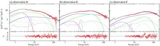
Unabsorbed, deconvolved spectra of observations D–F fitted with ‘tbabs*(diskbb+kdblur*xilconv*(nthcomp+nthcomp)+Gaussian)’. diskbb, higher and lower temperature nthcomp components are coloured with magenta, blue, and green, respectively. The reflected emissions of two nthcomp are shown with blue and green dotted lines. The model components are based on the best-fitting parameters shown in Table B2.
| Obs. | D | E | F |
|---|---|---|---|
| state | HIMS2 | HIMS1 | hard |
| Parameters of diskbb | |||
| kTin(keV) | |$0.68^{+0.03}_{-0.04}$| | 0.78 ± 0.08 | |$0.81^{+0.16}_{-0.21}$| |
| rin(rg) | |$46^{+10}_{-4}$| | <6.8 | |$8.1^{+8.3}_{-1.2}$| |
| Parameters of nthcomp | |||
| Γ | |$2.00^{+0.06}_{-0.00*}$| | |$2.00^{+0.03}_{-0.00*}$| | |$1.710^{+0.018}_{-0.016}$| |
| kTe(keV) | (300)† | (300)† | |$63^{+28}_{-13}$| |
| Norm | |$0.77^{+2.60}_{-0.06}$| | |$1.29^{+0.17}_{-0.10}$| | |$0.67^{+0.04}_{-0.08}$| |
| Γ | |$2.242^{+0.018}_{-0.014}$| | |$1.750^{+0.015}_{-0.029}$| | |$1.4^{+0.04}_{-0.00*}$| |
| kTe(keV) | |$11.4^{+0.9}_{-1.5}$| | |$9.22^{+0.17}_{-0.34}$| | 11.2 ± 0.7 |
| Norm | |$4.5^{+0.4}_{-1.5}$| | |$1.06^{+0.05}_{-0.09}$| | |$0.099^{+0.049}_{-0.013}$| |
| Parameters of kdblur, xilconv, and Gaussian | |||
| rref, in(rg) | |$30^{+21}_{-11}$| | |$25^{+36}_{-9}$| | |$13^{+8}_{-5}$| |
| rel_refl | 0.67 ± 0.06 | 0.51 ± 0.06 | |$0.53^{+0.06}_{-0.07}$| |
| Ec (keV) | |$6.20^{+0.05}_{-0.00*}$| | 6.31 ± 0.09 | |$6.26^{+0.09}_{-0.00*}$| |
| σ (keV) | (0.3)† | (0.3)† | (0.3)† |
| norm (× 10−3) | 17 ± 6 | |$14^{+4}_{-2}$| | |$6.2^{+1.5}_{-1.7}$| |
| EW (eV) | 59 ± 21 | |$75^{+21}_{-11}$| | |$74^{+18}_{-20}$| |
| χ2 (dof) | 83.2 (114) | 106.6 (114) | 134.4 (113) |
| χ2 (dof)|$^\#$| | 104.1 (116) | 145.0 (116) | 160.4 (115) |
| F-value|$^\#(\Delta$|dof) | 14.3( 2) | 20.5 (2) | 10.9 (2) |
APPENDIX C: THE sssed FITS WITH BLURRED REFLECTION
To observe the difference between using smedge and full reflection continuum, we attempted to fit the six sample spectra by replacing smedge with the fully ionized reflection code xilconv. The Gaussian component remained statistically important, similar to the case of the canonical diskbb and nthcomp fit with reflection in Appendix B. The resulting xspec model is:
The parameters used for xilconv and kdblur were the same as in Appendix B. The reflection component was blurred using kdblur model which describes the general relativistic blurring with β = −3 and rref, out = 400rg. Since the value of σ of Gaussian was not well constrained for observations B–F, we fixed it to be 0.3 keV, and constrained to be 0.1–0.8 keV for observation A. Additionally, except for observations A and B, the best-fitting value of the inner radius for the reflection rref, in was consistent with rcor of SSsed within 90 per cent uncertainties when it was remained as a free parameter. Therefore, we tied rref, in to rcor for observations C–F. Similar to the approach taken with the phenomenological smedge fit, the inner radius was fixed at 4.5rg for observations C–F, even though slightly larger rin was estimated for observation B (the SIMS). Additionally, kTe of the thermal Comptonizing component was fixed at 9 keV for observations B and C.
C1 Summary
The unabsorbed spectra with the best-fitting reflection continuum (plus Gaussian) are shown in figs c1a–f based on the best-fitting parameters shown in table c1. The model with the reflection continuum and a Gaussian successfully reproduced the spectra for observations B–E (the SIMS and HIMS). As discussed in Sections 4.2–4.3, the geometry parameters of rin and rcor obtained with full reflections were consistent with those approximately obtained by using smedge.

The best-fitting parameters of ’tbabs*(SSsed+kdblur*xilconv*SSsedcoronae+Gaussian)’. *The fitting values reach their lower or upper limits. † The values in the parentheses are fixed. |${^\S}$|The inner radius for reflection is tied to rcor. ‡The values of iron abundance, outer radius for reflection and inclination angle are fixed at nominal values: i.e. ZFe = 1, rref, out = 400rg, ixilconv = 75○. |$^\#$|Same as Tables B1 and B2, Chi-squared values for the same fits without Gaussian component, and F-values calculated as |$F=(\Delta \chi ^2/\chi ^2_\nu)/\Delta \nu$|, representing the improvement due to the Gaussian component.
| Obs. | A | B | C | D | E | F |
|---|---|---|---|---|---|---|
| state | soft | SIMS | HIMS3 | HIMS2 | HIMS1 | hard |
| Parameters of the SSsed | ||||||
| |$\log \dot{m}$| | |$0.137^{+0.001}_{-0.013}$| | 0.36 ± 0.03 | 0.206 ± 0.003 | 0.204 ± 0.006 | 0.037 ± 0.009 | |$-0.097^{+0.013}_{-0.014}$| |
| rin (rg) | |$5.37^{+0.04}_{-0.02}$| | |$4.64^{+0.24}_{-0.29}$| | (4.5)† | (4.5)† | (4.5)† | (4.5)† |
| rcor (rg) | |$6.702^{+0.042}_{-0.010}$| | |$9.3^{+0.8}_{-0.9}$| | |$10.72^{+0.08}_{-0.07}$| | |$13.36^{+0.17}_{-0.14}$| | |$23.8^{+1.7}_{-0.7}$| | |$27.3^{+1.2}_{-1.1}$| |
| Γth | — | |$4.0^{+0.0}_{-0.6}$| | |$2.62^{+0.11}_{-0.06}$| | |$2.258^{+0.011}_{-0.143}$| | |$1.80^{+0.05}_{-0.07}$| | |$1.400^{+0.016}_{-0.000*}$| |
| kTe (keV) | — | (9)† | (9)† | |$11.1^{+0.9}_{-2.3}$| | |$9.8^{+0.3}_{-0.7}$| | |$12.8^{+0.4}_{-0.2}$| |
| Γnth | |$2.109^{+0.017}_{-0.009}$| | 2.26 ± 0.03 | 2.26 ± 0.08 | |$2.07^{+0.26}_{-0.07*}$| | |$2.0^{+0.05}_{-0.00*}$| | |$1.774^{+0.009}_{-0.013}$| |
| kTe (keV) | (300)† | (300)† | (300)† | (300)† | (300)† | |$198^{+102*}_{-90}$| |
| fth | (0)† | |$0.31^{+0.05}_{-0.03}$| | |$0.25^{+0.10}_{-0.07}$| | |$0.67^{+0.07}_{-0.31}$| | |$0.47^{+0.02}_{-0.08}$| | |$0.208^{+0.017}_{-0.019}$| |
| Parameters of kdblur‡, xilconv‡, and Gaussian | ||||||
| rref, in (rg) | |$2.2^{+0.5}_{-0.4}$| | |$6.8^{+1.3}_{-1.8}$| | (10.72)|${^\S}$| | (|$13.36)^{\S}$| | (23.8)|$^{\S}$| | (27.3)|$^{\S}$| |
| rel_refl | |$2^{+0.0*}_{-0.3}$| | |$0.97^{+0.26}_{-0.10}$| | |$1.0^{+0.00*}_{-0.05}$| | 0.86 ± 0.08 | |$0.69^{+0.07}_{-0.10}$| | 0.68 ± 0.07 |
| Ec (keV) | |$6.62^{+0.07}_{-0.08}$| | |$6.31^{+0.12}_{-0.11*}$| | |$6.21^{+0.08}_{-0.00*}$| | |$6.23^{+0.07}_{-0.03*}$| | |$6.24^{+0.11}_{-0.04*}$| | |$6.20^{+0.12}_{-0.00*}$| |
| σ (keV) | |$0.80^{+0.00*}_{-0.06}$| | (0.3)† | (0.3)† | (0.3)† | (0.3)† | (0.3)† |
| norm (× 10−3) | 7.1 ± 0.6 | |$16^{+4}_{-5}$| | 19 ± 2 | 26 ± 3 | 12 ± 2 | 2.1 ± 1.1 |
| EW (eV) | 200 ± 17 | |$56^{+14}_{-18}$| | 82 ± 9 | 96 ± 11 | 64 ± 11 | 24 ± 13 |
| χ2 (dof) | 156.5 (116) | 122.3 (115) | 103.3 (117) | 91.4 (116) | 93.0 (116) | 156.1 (115) |
| χ2 (dof)|$^\#$| | 638.7 (119) | 146.8 (117) | 276.2 (119) | 309.6 (118) | 158.2 (118) | 166.6 (117) |
| F-value|$^\#(\Delta$|dof) | 119.1 (3) | 11.5 (2) | 97.3 (2) | 138.4 (2) | 40.7 (2) | 3.9 (2) |
In addition, except for the hard state (observation F), the additional Gaussian component remained significant (see F-values in Table C1) and had an equivalent width of above 50 eV, indicating contributions from other locations such as winds, or very outer disc as suggested by Connors et al. (2020). Therefore, the smoothed edge structure that determines the reflection ratio is likely influenced by absorption lines and edges produced by such winds. Indeed, XTE J1550 − 564 is a highly inclined source, and the contribution from winds is expected to be significant. Complex absorption structures can be clearly observed in the 7–10 keV range, which vary with changes in ionization states. These complex absorption structures, when combined with the reflection structure, can lead to the possibility of overestimating the values of rel_refl, which were estimated to be relatively large as 0.7–1 (Table C1).
These issues could potentially be resolved with data sets of finer spectral resolution. However, the analysis performed with our RXTE data has already surpassed the intended scope of this paper, and a detailed investigation of absorption/reflection structures is beyond its focus. Instead–, we adopted a phenomenological approach using the smedge and Gaussian models and estimated the uncertainty without full reflection modelling to be less than 10 per cent and most likely around 5–8 per cent.
C2 The soft state and SIMS
The spectrum of observation A was not well reproduced (χ2 = 156.5 for degree of freedom of 116) and the model required large reflection continuum with rel_refl=2 (upper limit). The SIMS spectrum of observation B was well reproduced by replacing smedge with blurred reflection (see Tables 2 and C1), and the estimated values of rin and rcor are consistent with those estimated using smedge. On closer inspection, the best-fitting value of rin increased by 4 per cent from |$(4.4^{+0.4}_{-0.3}) r_{\rm g}$| to |$(4.6^{+0.2}_{-0.3})r_{\rm g}$|, while that of rcor decreased by 3 per cent from |$(9.6^{+1.1}_{-0.9})r_{\rm g}$| to |$(9.3^{+0.8}_{-0.9})r_{\rm g}$|.
C3 The HIMS
We again compare the results with smedge and with blurred reflection for the HIMS data of observations C, D and E (Table C1). The values of rcor were found to decrease from (11.9 ± 0.3)rg to |$(10.72^{+0.08}_{-0.07})r_{\rm g}$|, from |$(15.1^{+0.4}_{-0.6})r_{\rm g}$| to |$(13.4^{+0.1}_{-0.2})r_{\rm g}$|, and from |$(25^{+2}_{-1})r_{\rm g}$| to |$(23.8^{+1.7}_{-0.7})r_{\rm g}$| for the fixed rin at 4.5rg, corresponding to decreases of 10 per cent, 11 per cent, and 5 per cent, respectively. If we consider 4 per cent increase in rin (see Section 4.2) and change the fixed value of rin from 4.5rg to 4.7rg, changes in rcor become only 6 per cent, 8 per cent, and 1 per cent, for observations C, D, and E, respectively.
C4 The bright hard state
In contrast to the SIMS and HIMS, the goodness of fit significantly deteriorated when we replaced smedge with the blurred reflection continuum for observation F (Table C1). Additionally, the electron temperature of the higher temperature Compton component was found to be much higher, exceeding >100 keV. Therefore, a more detailed analyses is required for the two thermal Comptonizations. However, the estimated value of rcor was consistent between smedge and reflection modellings, and detailed studies to investigate two-temperature Comptonization is beyond the scope of this paper.
APPENDIX D: POWER SPECTRAL DENSITY OF OBSERVATIONS A–F
Fig. D1 displays the PSDs in observations A–F, normalized to the average PCA count rate. In this figure, the PSDs were obtained in different energy bands, including 2–4.5 keV (orange), 4.5–15 keV (green), 15–34 keV (blue), and 34–120 keV (purple). The PSDs of 2–15 and 15–120 keV were obtained using binned mode and event mode, respectively.
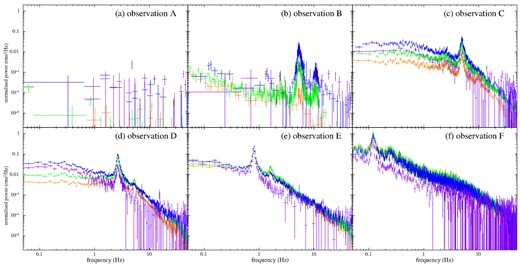
PSD normalized to average count rate for observations A–F, in the energy bands of 2–4.5 keV (orange), 4.5–15 keV (green), 15–34 keV (blue), and 34–120 keV (purple). The light curves in the energy range of 2–4.5, 4.5–15, 15–34, and 34–120 keV were extracted from PCA channels of 0–10 ch, 11–35 ch, 36–79 ch, and 80–255 ch, respectively.
These figures demonstrate that the soft state data of observations A does not exhibit any significant time variation, whereas the HIMS and hard state data of observations C–F exhibit significant intensity variations accompanied by strong Type-C QPOs. This is consistent with the association between the QPO types and spectral states shown e.g. by Motta et al. (2011). In the intermediate case of observation B, strong Type-B QPOs are clearly visible, while the overall variation remains negligible.
APPENDIX E: THE INNER RADII IN THE SIMS
Fig. E1 shows the evolution of the rin values with the SSsed model in the SIMS. The top panel shows rin, which is almost constant at 4.5rg.
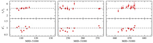
Time history of rin in the SIMS. The reduced chi-squared values are plotted in the bottom panels. Dashed lines represent rin = 4.5rg (top) and |$\chi ^2_\nu =1$| (bottom). Left, middle, and right panels correspond to red, orange, and cyan in Fig. 1.
