


ABSTRACT
X-ray properties of active galactic nuclei (AGNs) depend on their underlying physical parameters, particularly the accretion rate. We identified eight reverberation-mapped AGNs with some of the largest known accretion rates without high-quality X-ray data. We obtained new Chandra ACIS-S X-ray observations and nearly simultaneous optical spectrophotometry to investigate the properties of these AGNs with extreme super-Eddington accreting massive black holes (SEAMBHs). We combined our new X-ray measurements with those of other reverberation-mapped AGNs, which have the best-determined masses and accretion rates. The trend of the steepening of the spectral slope between X-ray and optical-UV, αox, with increasing optical-UV luminosity, |$L_{\rm 2500{\mathring{\rm A}}}$|, holds true for even the most extreme SEAMBHs. One of our new SEAMBHs appears X-ray-weak for its luminosity, perhaps due to absorption associated with orientation effects involving a slim disc thought to be present in highly accreting systems. The correlation of the |$\rm 2\!-\!8~ keV$| X-ray photon index with the accretion rate also holds for the extreme SEAMBHs, which show some of the largest photon indices reported for AGNs.
1 INTRODUCTION
Active galactic nuclei (AGNs) emit radiation across the entire electromagnetic spectrum due to various physical processes ultimately powered by the gravitational potential energy of the accreting supermassive black hole (Salpeter 1964; Pringle, Rees & Pacholczyk 1973; Ho 2008). The accreting matter forms a disc around the central supermassive black hole, which glows brightly in optical, UV, and soft X-rays. The spectral energy distribution (SED) of AGNs peaks in the UV emitted from the inner accretion disc. The Compton upscattering of optical-UV disc photons by the hot electrons in a region close (observations indicate three to few tens of gravitational radii, Sunyaev & Truemper 1979; McHardy et al. 2005; Chartas et al. 2016; Wilkins et al. 2016) to the black hole, called the corona, produces hard X-rays (e.g. Haardt & Maraschi 1991, 1993; Nakamura & Osaki 1993; Kawaguchi, Shimura & Mineshige 2001). Above 2 keV (in the range 2–100 keV), the X-ray spectrum is dominated by a single power-law continuum, N(E) ∝ E−Γ, with a high-energy cut-off (Sunyaev & Titarchuk 1980). Studies have found the cut-off energy is typically tens of keV or higher (Ricci et al. 2017; Molina et al. 2019; Tortosa et al. 2023). The photon index (Γ) acts as a tool to infer the energy distribution of the electrons in the corona. The two-point spectral index between 2500 |${\mathring{\rm A}}$| and 2 keV (αox, Tananbaum et al. 1979; Just et al. 2007) indicates the relative strength of the energy emitted by the disc versus the corona.
Past studies have examined the correlation between the X-ray-to-optical properties of quasars with various observed and fundamental properties. The photon index and αox generally show no variation with redshift (e.g. Page et al. 2005; Shemmer et al. 2005, 2006; Steffen et al. 2006; Just et al. 2007). However, αox exhibits a strong anticorrelation with optical-UV luminosity at 2500 |${\mathring{\rm A}}$| (Steffen et al. 2006; Just et al. 2007; Timlin et al. 2020). Steffen et al. (2006) find a 13.6σ correlation between αox and |$L_{2500{\mathring{\rm A}}}$| using a sample of 333 AGNs with redshifts up to z ∼ 6 and spanning over five orders of magnitude in |$L_{2500{\mathring{\rm A}}}$| and four orders of magnitude in X-ray luminosity. The αox–|$L_{2500{\mathring{\rm A}}}$| correlation is a by-product of the non-linear correlation between the luminosities at 2 keV and 2500 |${\mathring{\rm A}}$| (Vignali, Brandt & Schneider 2003; Strateva et al. 2005; Steffen et al. 2006; Just et al. 2007; Lusso et al. 2010; Young, Elvis & Risaliti 2010). It indicates AGNs with higher optical brightness emit relatively fewer X-rays than more optically faint AGNs (Lusso & Risaliti 2016). Through careful sample control, Lusso & Risaliti (2016) tightened the |$L_{2500{\mathring{\rm A}}}$|–|$L_{2 \rm ~ keV}$| relation, reducing the dispersion from ∼0.35–0.4 dex (from previous studies) to ∼0.21–0.24 dex seen in four orders of magnitude in luminosity. Such a tight correlation indicates that the energy emitted by the accretion disc and corona is inextricably linked. We also note that αox shows weak to no correlation with the Eddington ratio (e.g. Young, Elvis & Risaliti 2010).
A strong anticorrelation between Γ (both soft and hard photon index) and full width at half-maximum of H β emitted from the broad emission-line region (Wang, Brinkmann & Bergeron 1996; Brandt, Mathur & Elvis 1997; Laor et al. 1997; Wang, Watarai & Mineshige 2004) indicates the dependence of X-ray properties on the fundamental properties of black holes like mass or accretion rate. This anticorrelation is likely a secondary effect of a more intrinsic correlation between hard Γ and the Eddington ratio (LBol/LEdd), a normalized accretion rate parameter (Shemmer et al. 2006, 2008; Brightman et al. 2013; Trakhtenbrot et al. 2017; Tortosa et al. 2023). As the accretion rate increases, the accretion disc heats up, glowing in soft X-rays and increasing the Compton cooling of the corona, resulting in a steepening and softening of the X-ray spectra (Shemmer et al. 2006, 2008). Therefore, X-rays are critical for probing the accretion process in the vicinity of black holes.
The correlation between the |$\rm 2\!-\!8~ keV$| photon index and Eddington ratio holds over a range of quasar luminosity and redshift. For example, Shemmer et al. (2008) combine the Shemmer et al. (2006) sample of 25 moderate luminosity (|$43 \lt {\rm log}~ \nu L_{\nu }(5100{\mathring{\rm A}}) [\rm erg~ s^{-1}] \le 46$|) and five high-luminosity (|$46 \lt {\rm log}~ \nu L_{\nu }(5100{\mathring{\rm A}}) [\rm erg~ s^{-1}] \le 48$|) type-1 radio-quiet quasars at z < 0.5 and z ∼ 2, respectively, with five high-luminosity quasars at z = 1.3–3.2. These 35 quasars have high-quality optical spectra to derive black hole mass estimates based on the H-beta line and high-quality X-ray spectra to measure Γ. Although the sample was not complete or necessarily representative, their results established a significant correlation between Γ2-8 keV and LBol/LEdd over four orders of magnitude in quasar luminosity. Risaliti, Young & Elvis (2009) studied ∼400 AGNs with good-quality optical spectra from SDSS and XMM–Newton X-ray observations from the SDSS/XMM–Newton quasar survey (Young, Elvis & Risaliti 2009) spanning three orders of magnitude in optical luminosity. Their results show a highly significant correlation between Γ2-8 keV and LBol/LEdd. Risaliti, Young & Elvis (2009) also find that the strength and significance of the Γ2-8 keV–LBol/LEdd correlation decreases going from H β to Mg ii to no correlation when C iv-based mass is used to calculate the Eddington ratio. Brightman et al. (2013) also confirmed the Γ2-8 keV–LBol/LEdd correlation using a sample of 69 type-1 radio-quiet AGNs with redshifts up to ∼2.1 with X-ray spectra from the Chandra Deep Field-South survey (Lehmer et al. 2005) and black hole mass estimates based on H α and Mg ii measurements from the Cosmic Evolution Survey (Cappelluti et al. 2009; Elvis et al. 2009). Using 71 type-1 AGNs selected from the XMM–Newton Bright Serendipitous survey, Fanali et al. (2013) found a significant correlation between |$\Gamma _{0.5-10~ \rm keV}$| and LBol/LEdd after removing the dependence on redshift. They found a less significant correlation with Γ2-8 keV due to a larger error in determining Γ2-8 keV, a factor of 2.5 larger compared to the error in |$\Gamma _{0.5-10~ \rm keV}$|.
The correlations like Γ2-8 keV–LBol/LEdd and |$\alpha _{\rm ox}\!-\!L_{2500{\mathring{\rm A}}}$| are evident for the sub-Eddington accreting (LBol/LEdd ≪ 1) sources. Quasars with low Eddington ratios presumably have an optically thick and geometrically thin accretion disc. In the standard Shakura & Sunyaev (1973) thin disc model, the spin of the black hole defines the innermost stable orbit that dictates the radiation efficiency (η). For a retrograde spin, η = 0.038, whereas for a maximally spinning black hole, η = 0.32. But in the case of a higher accretion rate, the accretion disc becomes geometrically thick or slim (Abramowicz et al. 1988; Laor & Netzer 1989; Wang & Zhou 1999; Wang et al. 2013). Due to effects like photon trapping and advection-dominated energy transport, the slim disc has significantly smaller radiation efficiency that may be independent of spin (Wang & Zhou 1999; Mineshige et al. 2000; Wang et al. 2013). The SED of a slim accretion disc is likely different from a thin disc with a cut-off at higher energies, although a comparison of IR-optical-UV-X-ray SEDs of super- and sub-Eddington RM AGNs shows no anomalous torus emission or a heightened ionizing continuum predicted for slim disc systems (Castelló-Mor, Netzer & Kaspi 2016; Castelló-Mor et al. 2017). Super-Eddington accreting AGNs exhibit optical-UV SEDs that align well with the standard thin disc model. Any indications of a slim disc may be present in the extreme ultra-violet (EUV) where data availability is limited (Castelló-Mor, Netzer & Kaspi 2016; Kubota & Done 2019).
Wang et al. (2014) suggested that high accreting objects likely have slim accretion discs and coined the acronym super-Eddington accreting massive black holes (SEAMBHs). They are characterized by large Eddington ratios (LBol/LEdd > 0.3). SEAMBHs deviate from the traditional radius–luminosity relationships established for the low-accreting AGNs of the form R ∝ L∼0.5 (e.g. Kaspi et al. 2000; Bentz et al. 2013). A dedicated RM campaign by Du et al. (2014, 2015, 2016, 2018) tested the R–L relationship for the most highly accreting AGNs. They selected SEAMBH candidates based on a dimensionless accretion rate estimator, |$\,\,\,\,\,\,\,\,{\dot{\mathscr {\!\!\!\!\!\! M}}}$|, such that a |$\,\,\,\,\,\,\,\,{\dot{\mathscr {\!\!\!\!\!\! M}}}\ge 3$| implies an SEAMBH. In the context of thin-discs, the Eddington ratio is related to |$\,\,\,\,\,\,\,\,{\dot{\mathscr {\!\!\!\!\!\! M}}}$| by the equation |$L_{\rm Bol}/L_{\rm Edd} = \eta \,\,\,\,\,\,\,\,{\dot{\mathscr {\!\!\!\!\!\! M}}}$| (Du et al. 2014, 2015). Here, η is the mass-to-radiation conversion efficiency, a parameter dependent on the black hole spin. Du et al. (2018) show that the highest accretion rate AGNs have systematically shorter time lags, a factor of 3–8 times smaller than predicted by the canonical R–L relationship for the sub-Eddington accreting AGNs. Slim accretion discs in SEAMBHs are perhaps responsible for the shortened time lags of the broad-line region (BLR), due to anisotropic emission from the ionizing source (Wang et al. 2014; Du & Wang 2019). The canonical single-epoch black hole masses of highly accreting quasars are overestimated, on average, by a factor of 2 and the accretion rate parameters LBol/LEdd and |$\,\,\,\,\,\,\,\,{\dot{\mathscr {\!\!\!\!\!\! M}}}$| consequently underestimated (Maithil et al. 2022). SEAMBHs are not so common at low redshift but their fraction is expected to be higher in the early Universe (Kelly & Shen 2013). Discoveries of billion solar mass black holes at z > 6, when the Universe was less than a billion years old, are suggestive of super-Eddington accretion (e.g. review by Valiante et al. 2017 and references therein). Thus, SEAMBHs are probes to understand the accretion process and disc–corona connection of the high-redshift massive highly accreting AGNs.
Recently, Liu et al. (2021) probed the disc–corona connection using a sample of 26 sub-Eddington and 21 super-Eddington accreting AGNs. They used the most accurate reverberation-mapped black hole masses eliminating a major source of uncertainty in the Γ2-8 keV–LBol/LEdd correlations coming from the black hole mass estimates used to derive the Eddington ratio. Other intrinsic differences between AGNs like black hole spin, orientation, and optical depth in the corona likely also contribute to uncertainties in such relations. Most of the past studies were limited to sub-Eddington sources and used the single-epoch black hole mass scaling relations for broad-emission lines like H β, H α, and Mg ii based on the traditional R–L relationships. Some studies looked at X-ray and optical-UV properties of super-Eddington accreting sources but they did not perform a comparative investigation with the sub-Eddington sources (e.g. Ai et al. 2011; Kamizasa, Terashima & Awaki 2012). In this paper, we extend the investigations of Liu et al. (2021) by adding 13 extreme SEAMBHs from the SEAMBH-RM campaign that show the highest accretion rates (log |$\,\,\,\,\,\,\,\,{\dot{\mathscr {\!\!\!\!\!\! M}}}\gt 1.5$|) and the largest deviation in the BLR sizes from the canonical R–L relationship. We present the Chandra X-ray data of eight SEAMBHs for the first time with simultaneous optical-UV spectra avoiding uncertainties in the derivation of αox due to variability. Our work tests whether the extreme SEAMBHs follow the trends seen in sub- and super-Eddington accreting AGNs. In Section 2, we describe our sample and summarize the sample selection of Liu et al (2021). Section 3 presents the data reduction and analysis of our new Chandra observation and the optical-UV spectra. This is followed by an explanation of measured and derived quantities in Section 4. Section 5 presents the key results and Section 6 presents the discussion and conclusion. Throughout the paper, we adopt a cosmology with H0 = 70 km s−1 Mpc−1, ΩΛ = 0.7, and Ωm = 0.3.
2 SAMPLE
The reverberation mapping of SEAMBHs by Du et al. (2018) leads to the identification of 14 SEAMBHs that have markedly smaller BLR sizes than expected from their luminosities and have extreme accretion rates, i.e. log |$\,\,\,\,\,\,\,\,{\dot{\mathscr {\!\!\!\!\!\! M}}}\gt 1.5$|. Our core sample consists of these 14 ‘extreme SEAMBHs’.
Eight of these extreme SEAMBHs did not have X-ray observations above 2 keV (called ‘Chandra SEAMBHs’). We proposed Chandra Advanced CCD Imaging Spectrometer (ACIS-S) observations of these eight SEAMBHs in Cycle 20. We used the timed exposure ACIS operation mode with the faint telemetry format. To mitigate potential pile-up issues, we used the one-eight sub-array with only the S3 chip turned on. The spectral coverage of Chandra allows us to measure both the 2–8 keV X-ray photon index (|$\Gamma _{2-8~ \rm keV}$|) and, combined with optical-UV data, the αox. To minimize the effect of variability in αox measurements, the Chandra observations were accompanied by ground-based optical-UV spectral observations as close in time as weather permitted using the Lijiang 2.4 m and the Calar Alto 2.2 m telescopes. We present the X-ray and optical-UV data reduction and analysis in the next section. Table 1 provides the observation log of our Chandra targets.
Sample properties and observation log of the eight extreme SEAMBHs selected for Chandra observation and one Archived SEAMBH.
| Chandra X-ray | Optical | ||||||||
|---|---|---|---|---|---|---|---|---|---|
| Object | z | NH | log MBH | log |$\,\,\,\,\,\,\,\,{\dot{\mathscr {\!\!\!\!\!\! M}}}$| | ObsID | Date | Exposure time | Observatory | Date |
| (|$10^{20} \rm cm^{-2}$|) | (M⊙) | (s) | |||||||
| IRAS04416+1215 | 0.09 | 15.45 | 6.78 | 2.63 | 21510 | 2018-10-23 | 3466.68 | Lijiang | 2018-10-25 |
| SDSSJ074352.02+271239.5 | 0.25 | 4.24 | 7.93 | 1.69 | 21511 | 2018-10-27 | 4551.67 | CAHA | 2018-11-04 |
| SDSSJ080131.58+354436.4 | 0.18 | 4.90 | 6.51 | 2.43 | 21512 | 2018-12-16 | 7350.62 | Lijiang | 2018-12-19 |
| SDSSJ083553.46+055317.1 | 0.20 | 3.19 | 6.87 | 2.41 | 21513 | 2019-01-15 | 8558.59 | CAHA | 2019-01-17 |
| SDSSJ084533.28+474934.5 | 0.30 | 2.96 | 6.76 | 2.76 | 21514 | 2019-01-12 | 17319.36 | Lijiang | 2019-01-18 |
| SDSSJ093302.68+385228.0 | 0.18 | 1.44 | 7.08 | 1.79 | 21515 | 2019-01-19 | 10897.60 | Lijiang | 2019-01-24 |
| SDSSJ100402.61+285535.3 | 0.33 | 2.09 | 7.44 | 2.89 | 21516 | 2018-11-18 | 6311.02 | Lijiang | 2018-11-20 |
| SDSSJ101000.68+300321.5 | 0.26 | 2.27 | 7.46 | 1.70 | 21517 | 2019-01-23 | 9864.07 | Lijiang | 2019-01-25 |
| SDSSJ075051.72+245409.3a | 0.40 | 5.32 | 7.67 | 2.14 | 24 723 | 2021-03-29 | 3387.21 | ... | ... |
Notes. Redshift, black hole mass, and dimensionless accretion rate measurements are from Du & Wang (2019). Galactic neutral hydrogen column density (NH) is from Dickey & Lockman (1990). Chandra exposure time (or LIVETIME) is the ONTIME corrected for average dead time corrections.
aThis target, observed by Chandra (PI: Gordon Garmire), is analysed in this paper and is part of the Archived SEAMBHs subsample.
The remaining six extreme SEAMBHs have archival data from Chandra, XMM–Newton, and Swift. SDSSJ075051.72+245409.3 has archival ASIC-S Chandra observation from Cycle 21 (PI: Gordon Garmire, see Table 1 for details). In the absence of simultaneous optical-UV observation for this target, we use |$L_{2500{\mathring{\rm A}}}$| measurement from Shen et al. (2011). SDSS J080101.41+184840.7, SDSS J093922.89+370943.9, IRAS F12397+3333, and PG 2130+099 have simultaneous X-ray observations from the XMM–Newton’s European Photon Imaging Camera-PN and MOS detectors and optical-UV observations from the Optical Monitor. Lastly, Mrk 142 is observed simultaneously in the X-ray and the UV-Optical using the Swift observatory. Throughout this paper, we refer to these six extreme SEAMBHs as ‘Archived SEAMBHs’. Except for SDSSJ075051.72+245409.3, the other five extreme SEAMBHs are part of the Liu et al. (2021) sample and we refer readers to their section 2 for details of X-ray and optical-UV analysis. We process the X-ray data of SDSSJ075051.72+245409.3 along with the eight Chandra SEAMBHs and present the details in Section 3.1.
We use the remaining Liu et al. (2021) sample of 16 super-Eddington (|$0.47 \lt {\rm log}\,\,\,\,\,\,\,\,{\dot{\mathscr {\!\!\!\!\!\! M}}} \lt 1.5$|) and 26 sub-Eddington accreting AGNs to complement our sample. Liu et al. (2021) selected radio-quiet RM AGNs from Du et al. (2015, 2016, 2018) that have good signal-to-noise archival X-ray data (S/N > 6 in the rest-frame >2 keV band) and simultaneous optical-UV observations. They eliminated AGNs that are heavily absorbed in X-rays due to outflows or display broad-absorption-line features and reddening in their UV spectra. Three out of these 16 super-Eddington AGNs are part of our Chandra SEAMBHs. Liu et al. (2021) present the archival Swift (IRAS 04416+1215, SDSS J074352.02+271239.5) and XMM–Newton (SDSS J100402.61+285535.3) data of these in-common targets. As X-rays can vary, we present the archival data of these three targets as part of the Liu et al. (2021) super-Eddington sample and treat them as separate measurements. Fig. 1 shows the |$L_{5100{\mathring{\rm A}}}-z$| plane for our 14 extreme SEAMBHs and the Liu et al. (2021) sample, adding more data points at z > 0.16. Our extreme SEAMBHs have log |$L_{5100 {\mathring{\rm A}}}\gt 43.3$| placing them at the luminous end of the super-Eddington AGNs studied previously.
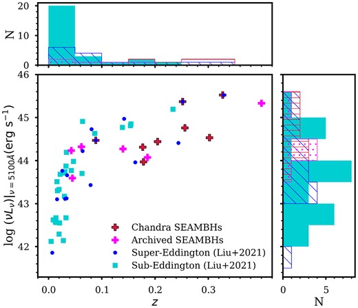
Monochromatic luminosity at 5100 |${\mathring{\rm A}}$| as a function of redshift. The plot shows the redshift–luminosity space spanned by our sample.
3 DATA REDUCTION AND ANALYSIS
3.1 Chandra X-ray reduction and spectral analysis
This paper presents Chandra data made available after CXC’s fifth reprocessing campaign. We analysed data using chandra interactive analysis of observations software (ciao) v4.13 (Fruscione et al. 2006). The level 1 event files were reprocessed using the chandra_repro script with caldb v4.9.5 to create the level 2 event files and observation-specific bad pixel files. We extracted the net counts, i.e. source counts minus background counts from the level 2 event file. To extract source counts we used a circular aperture of 4 arcsec (2 arcsec for SDSS J074352.02+271239.5) at the source coordinate, whereas an annulus with an inner radius of 8 arcsec (5 arcsec) and an outer radius of 13 arcsec (10 arcsec) was used to extract the background counts. The source and background regions were saved for later use in spectral analysis. The net counts were obtained in three bands: hard (2–8 keV), soft (0.35–2 keV), and broad (0.35–8 keV). Using these counts we calculated the hardness ratio defined as (Hard-Soft)/(Hard + Soft). Table 2 lists the photon counts and hardness ratio. Six out of eight Chandra SEAMBHs show a negative hardness ratio implying soft spectra, whereas two (SDSS J074352.02+271239.5 and SDSS J101000.68+300321.5) show hard spectra. One Archived SEAMBH with Chandra data, SDSSJ075051.72+245409.3, presents a soft spectrum.
Photon counts in broad, hard, and soft energy bands, and the hardness ratio.
| Object | Broad-band | Hard band (H) | Soft band (S) | Hardness ratio |
|---|---|---|---|---|
| (0.35–8 keV) | (2–8 keV) | (0.35–2 keV) | (H-S)/(H + S) | |
| IRAS04416+1215 | 1291.71 ± 35.98 | 474.08 ± 21.80 | 817.63 ± 28.62 | −0.27 |
| SDSSJ074352.02+271239.5 | 245.58 ± 15.69 | 143.90 ± 12.00 | 101.69 ± 10.10 | 0.17 |
| SDSSJ080131.58+354436.4 | 1015.00 ± 31.86 | 188.00 ± 13.71 | 827.00 ± 28.76 | −0.63 |
| SDSSJ083553.46+055317.1 | 1356.97 ± 36.88 | 322.64 ± 18.01 | 1034.33 ± 32.19 | −0.52 |
| SDSSJ084533.28+474934.5 | 390.48 ± 19.86 | 108.16 ± 10.50 | 282.32 ± 16.86 | −0.45 |
| SDSSJ093302.68+385228.0 | 452.87 ± 21.34 | 111.48 ± 10.64 | 341.39 ± 18.50 | −0.51 |
| SDSSJ100402.61+285535.3 | 610.01 ± 24.74 | 157.24 ± 12.57 | 452.78 ± 21.31 | −0.48 |
| SDSSJ101000.68+300321.5 | 72.69 ± 8.68 | 49.31 ± 7.16 | 23.38 ± 4.91 | 0.36 |
| SDSSJ075051.72+245409.3 | 125.38 ± 11.23 | 36.69 ± 6.09 | 88.69 ± 9.44 | −0.41 |
We used specextract to create source and background spectra and the instrument response files with point source aperture correction to unweighted auxiliary response files. The saved circular source aperture and annulus background regions were used to extract the spectra. We used Sherpa (Freeman et al. 2001) to fit the spectral data. The source model employed is a one-dimensional power-law and an xspec photoelectric absorption model with the hydrogen column density frozen to the Galactic value (Dickey & Lockman 1990) in the source direction (xsphabs.abs1 * powlaw1d.p1). The data were grouped to 5–30 counts per bin depending on the net count of the object. We used the Levenberg–Marquardt optimization method with W-statistic for fitting the spectra of all objects. The W-statistic is equivalent of the Cash statistic (Cash 1979), appropriate when using background-subtracted source spectra of low-count sources and also works well for high-count sources (Kaastra 2017). Fig. 2 shows the best-fitting model for the observed-frame 0.35 to 8/(1 + z) keV spectra. The best-fitting parameter values for the photon index, |$\Gamma _{\rm 0.35-8~ \rm keV}$|, absorption-corrected rest-frame 0.35–8 keV flux, and the reduced statistics are presented in Table 3.


(a) Power-law fit with Galactic absorption to the observed-frame 0.35–8/(1 + z) keV spectra of six Chandra SEAMBHs. (b) Power-law fit with Galactic absorption to the observed-frame 0.35–8/(1 + z) keV spectra of two Chandra SEAMBHs, which shows harder spectrum above 2 keV. (c) Power-law fit with Galactic absorption to the observed-frame 0.35–8/(1 + z) keV Chandra spectrum of one Archived SEAMBH analysed in this paper.
X-ray and optical-UV properties of Chandra SEAMBHs and SDSSJ075051.72+245409.3 from Archived SEAMBHs.
| Object | Γ0.35-8 keV | f0.35-8 keV | W-stat/DOF | Γ2-8 keV | f2-8 keV | W-stat/DOF | f2 keV | log L2 keV | log |$L_{2500{\mathring{\rm A}}}$| | log |$\nu L_{5100{\mathring{\rm A}}}$| | αox | Δαox |
|---|---|---|---|---|---|---|---|---|---|---|---|---|
| |$\rm (erg~ s^{-1} cm^{-2})$| | |$\rm (erg~ s^{-1} cm^{-2})$| | |$\rm (erg~ s^{-1} cm^{-2}~ keV^{-1})$| | |$\rm (erg~ s^{-1}~ Hz^{-1})$| | |$\rm (erg~ s^{-1}~ Hz^{-1})$| | |$\rm (erg~ s^{-1})$| | |||||||
| (1) | (2) | (3) | (4) | (5) | (6) | (7) | (8) | (9) | (10) | (11) | (12) | (13) |
| IRAS04416+1215 | 2.13 ± 0.05 | 6.47E-12 | 41.3/38 | 2.03 ± 0.12 | 2.67E-12 | 29.5/32 | 1.07E-12 | 25.90 | 29.67 | 44.47 | −1.45 | −0.02 |
| SDSSJ074352.02+271239.5a | 0.93 ± 0.13 | 8.09E-13 | 22.0/21 | 1.98 ± 0.53 | 8.97E-13 | 10.6/15 | 4.01E-13 | 26.41 | 30.57 | 45.37 | −1.60 | −0.05 |
| SDSSJ080131.58+354436.4 | 3.20 ± 0.07 | 3.77E-12 | 53.3/30 | 2.48 ± 0.18 | 4.55E-13 | 10.3/7 | 2.68E-13 | 25.92 | 29.17 | 43.97 | −1.24 | 0.11 |
| SDSSJ083553.46+055317.1 | 2.69 ± 0.05 | 3.08E-12 | 87.2/72 | 2.16 ± 0.13 | 7.38E-13 | 20.5/28 | 3.55E-13 | 26.17 | 29.69 | 44.44 | −1.35 | 0.08 |
| SDSSJ084533.28+474934.5 | 2.49 ± 0.10 | 3.85E-13 | 22.8/22 | 2.36 ± 0.22 | 1.13E-13 | 8.3/9 | 6.71E-14 | 25.80 | 29.37 | 44.53 | −1.37 | 0.01 |
| SDSSJ093302.68+385228.0 | 2.43 ± 0.10 | 6.84E-13 | 26.7/26 | 2.27 ± 0.22 | 2.03E-13 | 27.9/28 | 1.04E-13 | 25.51 | 29.36 | 44.31 | −1.48 | −0.09 |
| SDSSJ100402.61+285535.3 | 2.53 ± 0.08 | 1.64E-12 | 95.9/91 | 2.10 ± 0.16 | 5.06E-13 | 13.6/12 | 2.58E-13 | 26.45 | 30.54 | 45.52 | −1.57 | −0.02 |
| SDSSJ101000.68+300321.5a | 0.54 ± 0.24 | 1.16E-13 | 14.9/13 | 1.54 ± 1.03 | 1.31E-13 | 8.4/10 | 4.26E-14 | 25.45 | 29.81 | 44.76 | −1.67 | −0.23 |
| SDSSJ075051.72+245409.3 | 2.38 ± 0.19 | 7.46E-13 | 49.8/50 | 2.39 ± 0.31 | 2.61E-13 | 38.7/32 | 1.71E-13 | 26.45 | 30.41 | 45.33 | −1.52 | 0.01 |
Note.aWe fit the observed-frame 2/(1 + z) to 8/(1 + z) keV spectra of SDSS J074352.02+271239.5 and SDSS J101000.68+300321.5 using a power-law model incorporating both Galactic and intrinsic absorption. The best-fitting model indicates intrinsic absorption, with |$N_{\rm H} = \rm 3.5\times 10^{22}~ cm^{-2}$| and |$\rm 3.1\times 10^{22}~ cm^{-2}$| for SDSS J074352.02+271239.5 and SDSS J101000.68+300321.5, respectively.
Next, we fit the observed-frame 2/(1 + z) to 8/(1 + z) keV X-ray band, where the underlying spectrum is mostly free of absorption or soft-excess emission (Shemmer et al. 2006, 2008; Risaliti, Young & Elvis 2009; Brightman et al. 2013). Six Chandra SEAMBHs and the Archived SEAMBH (SDSSJ075051.72+245409.3) show soft, steep spectra well fit using a power-law model with Galactic absorption. SDSS J074352.02+271239.5 and SDSS J101000.68+300321.5 appear as outliers and have much harder spectra than the other SEAMBHs. We fit their spectra using a power-law model with both Galactic and intrinsic absorption (xsphabs.abs1 * xszphabs.zabs1 * powlaw1d.p1). SDSS J101000.68+300321.5 likely needs a more complex model, but the low photon count prevents us from uniquely doing so. For IRAS 04416+1215, we also adopted a high-energy cut-off for the power-law fixed to 44 keV from Tortosa et al. (2023). An F-test reveals that adding a high-energy cut-off does not improve the statistics significantly. We tested the presence of intrinsic absorption for each source. Except for SDSS J074352.02+271239.5, an F-test confirms that adding intrinsic absorption component to the Galactic-absorbed power-law model does not improve the fit significantly. Table 3 reports the |$2-8~ \rm keV$| photon index (Γ2-8 keV), the absorption-corrected rest-frame 2–8 keV flux, reduced statistics, and the monochromatic flux density at rest-frame energy of 2 keV from the best-fitting models. It should be noted that the rest-frame |$2-8~ \rm keV$| best-fitting values are the key X-ray results that we will use in our analysis. We provide the literature values of the photon index for IRAS 04416+1215, SDSS J074352.02+271239.5, SDSS J100402.61+285535.3, and SDSSJ075051.72+245409.3 in the Appendix A.
To assess absorption or excess in the soft (|$\lt 2~ \rm keV$|) X-ray band, we extrapolate the |$\rm 2-8~ keV$| X-ray power-law model to the observed-frame 0.35 to 2/(1 + z) keV energies. Nearly half of our targets exhibit soft excesses, with exceptions being SDSS J074352.02+271239.5, SDSS J084533.28+474934.5, SDSS J093302.68+385228.0, and SDSS J075051.72+245409.3. We tested three models to better describe their |$\lt 2~ \rm keV$| X-ray emission spectrum. Model 1 comprises a simple power-law with Galactic absorption. Model 2 includes a thermal Comptonization (xscomptt) component with a fixed underlying power-law using parameters from the |$\rm 2-8~ keV$| X-ray analysis presented in Table 3. Model 3 includes an additional partial covering ionized absorption component (ZXIPCF) into the fitting to account for weak absorption in the soft (|$\lt 2~ \rm keV$|) X-rays. For SDSSJ074352.02+271239.5, SDSSJ084533.28+474934.5, J093302.68+385228.0, and SDSS J075051.72+245409.3, the F-test indicates that fitting the |$\lt 2~ \rm keV$| band with a Galactic absorbed power-law model yields results similar to extending the |$\rm 2\!-\!8~ keV$| best-fitting to softer energies. Only for IRAS 04416+1215, SDSSJ080131.58+354436.4, SDSSJ083553.46+055317.1, SDSSJ100402.61+285535.3, and SDSSJ101000.68+300321.5, Model 1 emerges as the best fit. Table 4 gives the 0.35–2/(1 + z) keV photon index, absorption-corrected rest-frame 0.35–2 keV flux and statistics of the best-fitting model.
Best-fitting values for |$\lt 2\rm ~ keV$| X-ray spectral fitting.
| Object | Model | Γ0.35-2keV | f0.35-2 keV | W-stat/DOF |
|---|---|---|---|---|
| |$\rm (erg~ s^{-1} cm^{-2})$| | ||||
| IRAS04416+1215 | 1 | 2.52 ± 0.14 | 4.84E-12 | 30.9/36 |
| SDSSJ074352.02+271239.5a | – | 11.98 | 2.31E-13 | 10.7/11 |
| SDSSJ080131.58+354436.4 | 1 | 3.51 ± 0.11 | 4.19E-12 | 61.9/54 |
| SDSSJ083553.46+055317.1 | 1 | 3.12 ± 0.11 | 3.18E-12 | 36.4/43 |
| SDSSJ084533.28+474934.5a | – | 2.36 | 2.56E-13 | 15.2/17 |
| SDSSJ093302.68+385228.0a | – | 2.27 | 4.46E-13 | 19.8/16 |
| SDSSJ100402.61+285535.3 | 1 | 3.27 ± 0.18 | 1.82E-12 | 25.8/26 |
| SDSSJ101000.68+300321.5 | 1 | 3.10 ± 1.10 | 4.08E-14 | 6.6/6 |
| SDSSJ075051.72+245409.3a | – | 2.39 | 4.74E-13 | 5.8/6 |
Note. aFor these targets extending 2–8 keV Galactic-absorbed power-law model (see Table 3) to |$\lt 2\rm ~ keV$| energies gives the best-fitting results.
3.2 Optical spectral analysis
We obtained the optical spectra of the eight Chandra SEAMBHs almost simultaneously with the X-ray observations, using the Lijiang and/or CAHA observatories. Multiple observations with two sets of spectra were taken within 2–8 d of the Chandra observations. We selected the best-quality spectra closest in time to the Chandra observation.
For the six objects observed with the Lijiang 2.4 m telescope (listed in Table 1), their spectra were taken under the same settings of the grism and slit width as they were observed by Hu et al. (2015) (for IRAS 04416+1215), Du et al. (2015) (for SDSS J080131.58+354436.4), and Du et al. (2018) (for the other four objects). For the two objects observed at CAHA 2.2m telescope, the spectra were taken using the Calar Alto Faint Object Spectrograph with Grism G-200 and a slit set at a width of 3|${_{.}^{\prime\prime}}$|0, as described in Hu et al. (2021). For all the objects, the same comparison stars were taken simultaneously by rotating the slit, as they were monitored for reverberation mapping measurements. The data were reduced first by the standard procedures, including bias-removal, flat-field correction, wavelength calibration, and spectral extraction. Then the flux calibration was performed using a sensitivity function obtained from the simultaneously observed comparison star spectrum as in the previous reverberation mapping observations (see e.g. Hu et al. 2021 for the details of the method). Thus the flux here can be compared directly with those in the light curves of their previous reverberation mapping observations (Du et al. 2015, 2018; Hu et al. 2015).
We dereddened the mean spectra and fit a slope to the continuum around the H β region. The slope was extrapolated to get the monochromatic luminosities at a rest-frame wavelength of 2500 |${\mathring{\rm A}}$| luminosity for each target.
4 MEASURED AND DERIVED QUANTITIES
The broad-band photon index (Γ0.358 kev) is obtained from the best-fitting model at the observed-frame 0.35–8/(1 + z) keV energy band and the Γ2-8 keV in the observed-frame 2/(1 + z) to 8/(1 + z) keV energy band. The absorption-corrected rest-frame fluxes (f0.35-8 keV, f2-8 keV) were also obtained from these best-fitting models. We also obtained the monochromatic flux density at rest-frame 2 keV (f2keV) from the fitting of |$\rm 2\!-\!8~ keV$| energy band. The flux density (Fν) is converted to luminosity using |$L_{\nu } = 4 \pi D_{L}^2 F_{\nu }/(1+z)$| (e.g. Hogg et al. 2002).
- We used the following equation to derive αox:where f2 keV and |$f_{2500 {\mathring{\rm A}}}$| are X-ray (2 keV) and UV (2500|${\mathring{\rm A}}$|) monochromatic flux densities, respectively. A highly significant anticorrelation between αox and |$L_{2500{\mathring{\rm A}}}$| provides a method to predict αox based on |$L_{2500{\mathring{\rm A}}}$| measurement. We define Δαox as the difference between the measured αox and predicted from the Steffen et al. (2006) relation given as(1)$$\begin{eqnarray} \alpha _{\rm ox} = \frac{{\rm log} (f_{\rm 2~keV}/f_{2500 {\mathring{\rm A}}}) }{{\rm log} (\nu _{\rm 2~keV}/\nu _{\rm 2500 {\mathring{\rm A}}})} = 0.3838~ {\rm log} (f_{\rm 2~keV}/f_{2500 {\mathring{\rm A}}}) , \end{eqnarray}$$(2)$$\begin{eqnarray} \alpha _{\rm ox} = -(0.137\pm 0.008)~ {\rm log}~ L_{2500 {\mathring{\rm A}}} + (2.638\pm 0.240). \end{eqnarray}$$
- The black hole mass (MBH) is the H β reverberation-mapped mass. We use two accretion rate parameters: (a) The dimensionless accretion rate parameter |$\,\,\,\,\,\,\,\,{\dot{\mathscr {\!\!\!\!\!\! M}}}$| is defined aswhere m7 = MBH/107M⊙, |$\ell _{44} = L_{5100{\mathring{\rm A}}}/10^{44}$| is in units of |$\rm erg~ s^{-1}$| and i is inclination angle to the line of sight (we assumed a typical value of cos i = 0.75 for type-1 AGNs), (b) The Eddington ratio is defined as the ratio of bolometric luminosity (LBol) and Eddington luminosity (LEdd),(3)$$\begin{eqnarray} \,\,\,\,\,\,\,\,{\dot{\mathscr {\!\!\!\!\!\! M}}} = 20.1 \left(\ell _{44}/\cos i \right)^{3/2} m_7^{-2}, \end{eqnarray}$$For our Chandra SEAMBHs, we used new measurements of Γ2-8 keV, |$L_{2~ \rm keV}$|, and |$L_{2500{\mathring{\rm A}}}$| and calculated αox using equation (1). All the X-ray and optical-UV measurements for the Archival SEAMBHs, super-Eddington, and sub-Eddington samples were adopted from Liu et al. (2021). The monochromatic luminosity at |$5100~ {\mathring{\rm A}}$| (|$L_{5100{\mathring{\rm A}}}$|) and black hole properties MBH and |$\,\,\,\,\,\,\,\,{\dot{\mathscr {\!\!\!\!\!\! M}}}$| were taken from Du & Wang (2019) for all samples. Du & Wang (2019) computes |$\,\,\,\,\,\,\,\,{\dot{\mathscr {\!\!\!\!\!\! M}}}$| using |$L_{5100~{\mathring{\rm A}}}$| (see equation 3), whereas Liu et al. (2021) compute |$\,\,\,\,\,\,\,\,{\dot{\mathscr {\!\!\!\!\!\! M}}}$| using |$L_{2500{\mathring{\rm A}}}$|. Our choice of using the Du & Wang (2019) prescription for |$\,\,\,\,\,\,\,\,{\dot{\mathscr {\!\!\!\!\!\! M}}}$| results in two objects from the Liu et al. (2021) super-Eddington sample, PG 0953+414 and NGC 4748, to have |$\,\,\,\,\,\,\,\,{\dot{\mathscr {\!\!\!\!\!\! M}}}\lt 3$|. We count these two targets in the sub-Eddington sample. One target in the Liu et al. (2021) sub-Eddington sample, PG 0026+129, now has |$\,\,\,\,\,\,\,\,{\dot{\mathscr {\!\!\!\!\!\! M}}}\gt 3$|, and we count it in the super-Eddington sample. We calculate the Eddington ratio for all samples using equation (4), where we make a conservative choice of using the Richards et al. (2006) bolometric correction factor of 9.26 to estimate the bolometric luminosity (see Section 6 for further discussion).(4)$$\begin{eqnarray} L_{\rm Bol}/L_{\rm Edd} = \frac{9.26~ L_{5100{\mathring{\rm A}}}}{1.5 \times 10^{45}~ m_7~ {\rm erg~ s^{-1}}}. \end{eqnarray}$$
5 RESULTS
The distribution of 2–8 keV photon indices (Fig. 3) shows that extreme SEAMBHs typically exhibit steep photon indices, with Γ2-8 keV > 2. However, two Chandra SEAMBHs, SDSS J074352.02+271239.5 and SDSS J101000.68+300321.5, have Γ2-8 keV < 2. SDSS J101000.68+300321.5 has a low photon count (broad-band photon count of 72) and therefore the spectral fit is likely inaccurate. The Γ2-8 keV for the extreme SEAMBHs (|${\rm log}\,\,\,\,\,\,\,\,{\dot{\mathscr {\!\!\!\!\!\! M}}} \gt 1.5$|) ranges between 1.54 and 2.48 and has a mean value of 2.17 (2.22 excluding SDSS J101000.68+300321.5). In contrast, the mean Γ2-8 keV the for 15 super-Eddington AGNs (|$0.47 \lt {\rm log}\,\,\,\,\,\,\,\,{\dot{\mathscr {\!\!\!\!\!\! M}}} \lt 1.5$|) is 2.06, which is clearly distinct from the mean Γ2-8 keV of 1.81 for the sub-Eddington AGNs.
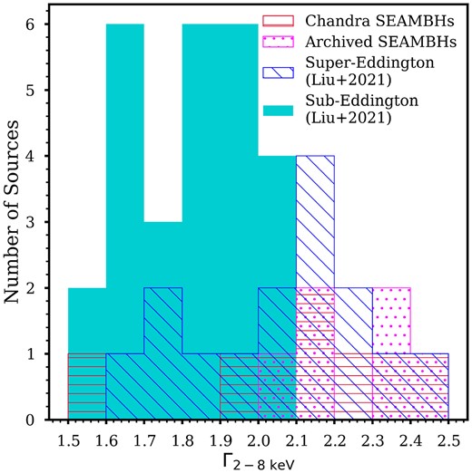
Histogram of the distribution of Γ2-8 keV for all samples. The sub-Eddington sources primarily have Γ2-8 keV < 2 with a mean value of 1.81, whereas the super-Eddington and extreme SEAMBHs samples span a wider range in Γ2-8 keV and have a mean value of 2.11.
Fig. 4 illustrates the αox versus |$L_{2500{\mathring{\rm A}}}$| plane. The αox values of extreme SEAMBHs range between −1.67 and −1.24, following the best-fitting linear regression from Steffen et al. (2006) as expressed in equation (2). The mean αox values are −1.46, −1.38, and −1.32 for the extreme SEAMBHs, super-Eddington, and sub-Eddington samples, respectively. αox tends to steepen with increasing |$L_{2500{\mathring{\rm A}}}$|, consistent with previous studies. We also plot the |$\alpha _{\rm ox}\!-\!L_{2500{\mathring{\rm A}}}$| best-fitting relationship from Timlin et al. (2020), given by αox = (−0.199 ± 0.011)log10(L2500) + (4.573 ± 0.333). Notably, this slope is significantly steeper than that of Steffen et al. (2006). Timlin et al. (2020) use a Bayesian linear regression method developed by Kelly (2007), while Steffen et al. (2006) utilize a bivariate data-analysis method presented in Isobe et al. (1990) for their best-fitting relations (see their respective papers for further details). Fig. 4 shows that the Timlin et al. (2020) relationship does not fit our sample very well, particularly at the low-luminosity end. Timlin et al. (2020) derived their relation from a sample of 753 quasars with |$29.3\lesssim {\rm log}~ L_{2500{\mathring{\rm A}}}\lesssim 31.6$|, spanning only two orders of magnitude. In contrast, the Steffen et al. (2006) relation is based on a sample of 293 quasars with |$28\lesssim {\rm log}~ L_{2500{\mathring{\rm A}}}\lesssim 33$|, covering four orders of magnitude. Given that the luminosity of our sample spans three orders of magnitude, |$27.2\lt {\rm log}~ L_{2500{\mathring{\rm A}}}\lt 30.7$|, it is more appropriate to use the Steffen et al. (2006) relationship to calculate Δαox.
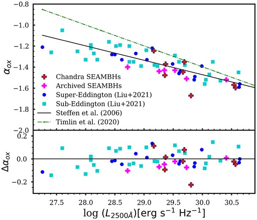
The top panel shows that αox becomes more negative with increasing |$L_{\rm 2500 {\mathring{\rm A}}}$| following the Steffen et al. (2006) relation represented by the black solid line. Our sample shows a large deviation from Timlin et al. (2020) relation, represented by the green dash–dot line, especially at the low luminosity end. The bottom panel plots Δαox as a function of |$L_{\rm 2500 {\mathring{\rm A}}}$|. A Δαox less than −0.2 implies significant X-ray weakness.
The bottom panel of Fig. 4 shows the residual between the measured αox and the expected value from Steffen et al. (2006) relation (as given in equation 2), plotted against |$L_{2500{\mathring{\rm A}}}$|. We plot the distribution of Δαox in Fig. 5. Luo et al. (2015) define Δαox = −0.2 as a threshold value, below which the AGN is considered X-ray-weak. Apart from one Chandra SEAMBH, Δαox varies between −0.15 and 0.15, typical for normal X-ray emission. Only SDSS J101000.68+300321.5 appears as X-ray-weak, with Δαox = −0.23. The limited photon count for this object hinders fitting more complex models to correct for absorption.
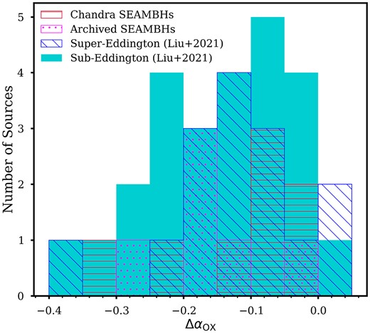
Histogram of the distribution of Δαox. Except for one extreme SEAMBH, SDSS J101000.68+300321.5, all sources appear X-ray normal.
Fig. 6 plots the best-fitting relation between |$L_{2~\rm keV}$| and |$L_{2500{\mathring{\rm A}}}$| for the super-Eddington sample (|${\rm log~} L_{2~\rm keV} = (0.73\pm 0.05)~ {\rm log~} L_{2500{\mathring{\rm A}}} + (4.3\pm 1.4)$|) and the sub-Eddington sample (|${\rm log~} L_{2~\rm keV} = (0.71\pm 0.05)~ {\rm log~} L_{2500{\mathring{\rm A}}} + (5.0\pm 1.5)$|) from Liu et al. (2021). These best-fitting relationships were derived using LINMIX_ERR method (Kelly 2007), which is a linear regression method that utilizes Bayesian priors for errors (refer to Liu et al. 2021 for further details). The slope of the Liu et al. (2021) best-fitting relation is within the error range of the typical value of 0.6 ± 0.1 seen in previous studies (e.g. Steffen et al. 2006; Lusso et al. 2010). The trend of suppression of X-ray emission in comparison to optical-UV emission holds for extreme SEAMBHs.
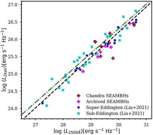
L2keV versus |$L_{\rm 2500 {\mathring{\rm A}}}$|. The black dashed (green dash–dotted) line represents the best-fitting relation for super-Eddington (sub-Eddington) sources from Liu et al. (2021). The plot shows that the non-linear correlation between X-ray and optical-UV luminosities is also present in extreme SEAMBHs.
5.1 Γ2-8 keV versus accretion rate
The |$\rm 2-8~ keV$| photon index is known to soften (steepen) with an increasing accretion rate. Shemmer et al. (2008) find a significant correlation between Γ2-8 keV and LBol/LEdd and derived a linear relation of the form Γ2-8 keV = a log LBol/LEdd + b, where the slope a = 0.31 and intercept b = 2.11. Subsequently, the Γ2-8 keV–LBol/LEdd correlation has been tested across AGNs spanning a wide range of luminosities and redshifts. For instance, Risaliti, Young & Elvis (2009) find a = 0.31 and b = 1.97 for their full sample, Brightman et al. (2013) report a = 0.32 and b = 2.27, and Fanali et al. (2013) find a = 0.25 and b = 2.48.
Fig. 7 illustrates the relationship between Γ2-8 keV and LBol/LEdd. It plots the best-fitting relation for the full sample from Liu et al. (2021) as Γ2-8 keV = (0.27 ± 0.04) log LBol/LEdd + (2.14 ± 0.04) in black, alongside the the Shemmer et al. (2008) relation, Γ2-8 keV = (0.31 ± 0.01) log LBol/LEdd + (2.11 ± 0.01), represented by a green dot–dashed line. Both the best-fitting relationships were derived using linear regression techniques that account for measurement errors. Liu et al. (2021) employed the LINMIX_ERR method (Kelly 2007), a Bayesian approach incorporating a prior distribution for errors. In contrast, Shemmer et al. (2008) utilized the bivariate correlated errors and scatter method (Akritas & Bershady 1996), which assumes random errors with no correlation. The extreme SEAMBHs follow the trend of steepening Γ2-8 keV as the Eddington ratio increases. The full sample shows a strong correlation between Γ2-8 keV and LBol/LEdd, with a Pearson r-coefficient of 0.70 and a probability p = 2.37E − 9. Removing the sub-Eddington sample weakens the Pearson correlation to r = 0.49, p = 0.01. We also tested the Spearman non-parametric correlation between the Γ2-8 keV and the Eddington ratio, yielding an r-coefficient = 0.70 and a probability p = 2.42E − 9 for the full sample. Without the sub-Eddington sample, the Spearman correlation decreases to r = 0.48, p = 0.01. A weak correlation between Γ2-8 keV and LBol/LEdd is observed for the 14 extreme SEAMBHs, with Pearson (Spearman) r = 0.29(0.33), p = 0.31(0.25). This may be be attributed to the shortcoming of a constant bolometric correction factor of 9.26 for estimating the bolometric luminosities in these highly accreting systems or, the small sample size, or the narrow range of LBol/LEdd and Γ2-8 keV spanned by the sample.
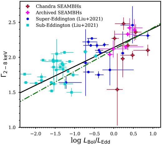
The plot Γ2-8 keV versus LBol/LEdd shows that Γ2-8 keV steepens with increasing accretion rate (Spearman r = 0.70, p = 2.42E-9). The green dash–dotted line represents the best-fitting relation from Shemmer et al. (2008) and the black solid line represents the best-fitting relation from Liu et al. (2021).
Using |$\,\,\,\,\,\,\,\,{\dot{\mathscr {\!\!\!\!\!\! M}}}$| as an accretion rate indicator is complementary to using the Eddington ratio, although these parameters are tightly correlated for AGNs. Fig. 8 plots Γ2-8 keV versus |$\,\,\,\,\,\,\,\,{\dot{\mathscr {\!\!\!\!\!\! M}}}$| for our full sample and displays the best-fitting relation from Liu et al. (2021) for their full sample, |$\Gamma _{\rm 2-8~ keV} = (0.15\pm 0.02)~ {\rm log}~ \,\,\,\,\,\,\,\,{\dot{\mathscr {\!\!\!\!\!\! M}}} + (1.91\pm 0.03)$|, in black. Again, Liu et al. (2021) employed the Bayesian linear regression method LINMIX_ERR (Kelly 2007), to derive the best-fitting relationship. The full sample shows a strong Pearson (Spearman) correlation between Γ2-8 keV and |$\,\,\,\,\,\,\,\,{\dot{\mathscr {\!\!\!\!\!\! M}}}$|, with r = 0.71 (0.72) and p = 5.80E − 10 (4.92E − 10). This correlation remains strong when the sub-Eddington sample is excluded, with Pearson (Spearman) r = 0.57(0.55) and p = 1.3E − 03(1.9E − 03). Γ2-8 keV and |$\,\,\,\,\,\,\,\,{\dot{\mathscr {\!\!\!\!\!\! M}}}$| correlate strongly with Pearson (Spearman) r = 0.46 (0.41) and p = 0.10 (0.14) for the extreme SEAMBHs. Our results confirm that the correlation between Γ2-8 keV and |$\,\,\,\,\,\,\,\,{\dot{\mathscr {\!\!\!\!\!\! M}}}$| extends to extreme SEAMBHs.

Γ2-8 keV versus |$\,\,\,\,\,\,\,\,{\dot{\mathscr {\!\!\!\!\!\! M}}}$|. The |$\rm 2-8~ keV$| photon index shows strong correlation with |$\,\,\,\,\,\,\,\,{\dot{\mathscr {\!\!\!\!\!\! M}}}$| (Spearman r = 0.72, p = 4.92E-10). The black solid line represents the best-fitting relation from Liu et al. (2021).
5.2 αox versus accretion rate and black hole mass
The physics behind the disc–corona connection responsible for the observed steepening of αox with increasing |$L_{2500{\mathring{\rm A}}}$| is not well understood (see Section 6 for further discussion). Past studies have investigated the connection between αox and black hole mass and accretion rate. A significant correlation is evident between αox and MBH (Done et al. 2012; Chiaraluce et al. 2018). However, there is only a weak or non-existent correlation between αox and LBol/LEdd (Vasudevan & Fabian 2007; Shemmer et al. 2008; Fanali et al. 2013), although Grupe et al. (2010) claim a strong correlation between them. The dependence of LBol on |$L_{2500{\mathring{\rm A}}}$| might be responsible for a weak correlation between αox and LBol/LEdd (Shemmer et al. 2008). Fanali et al. (2013) find a significant anticorrelation between αox and |$\,\,\,\,\,\,\,\,{\dot{\mathscr {\!\!\!\!\!\! M}}}$| for a sample of 71 type-1 AGNs using canonical single-epoch black hole masses to estimate |$\,\,\,\,\,\,\,\,{\dot{\mathscr {\!\!\!\!\!\! M}}}$|, which we now know suffer from accretion rate effects. Castelló-Mor et al. (2017) claim an anticorrelation between αox and |$\,\,\,\,\,\,\,\,{\dot{\mathscr {\!\!\!\!\!\! M}}}$| for 31 high-accretion rate sources (|$\,\,\,\,\,\,\,\,{\dot{\mathscr {\!\!\!\!\!\! M}}}$|>10) in their sample of 59 AGNs, using RM masses and an updated R–L relationship (Du et al. 2016) for high-accretion rate targets, although the correlation is limited by small number statistics. We examine the correlation between αox and |$\,\,\,\,\,\,\,\,{\dot{\mathscr {\!\!\!\!\!\! M}}}$| for our sample. Fig. 9 shows a slight anticorrelation (Pearson r = −0.45, p = 4.9E − 4) for the full sample, which weakens to Pearson (Spearman) r = −0.384(− 0.381), p = 3.99E − 2(4.16E − 2) when only |$\,\,\,\,\,\,\,\,{\dot{\mathscr {\!\!\!\!\!\! M}}}$|>3 AGNs are considered.
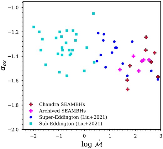
αox versus |$\,\,\,\,\,\,\,\,{\dot{\mathscr {\!\!\!\!\!\! M}}}$|. The plot shows a weak anticorrelation with Spearman r = −0.45, p = 5.1E-4 and weakens further if the sub-Eddington sample is excluded.
More recently, Liu et al. (2021) argue that αox depends on both LBol/LEdd and MBH, establishing a non-linear relationship of the form αox = (−0.13 ± 0.01) log LBol/LEdd − (0.10 ± 0.01) log MBH − (0.69 ± 0.09). They employed the Python package emcee (Foreman-Mackey et al. 2013), a tool for multivariate linear regression with Bayesian inference, to obtain this best-fitting relationship. More investigation is needed to decipher if this relation is fundamental or just a secondary manifestation of the αox–|$L_{2500{\mathring{\rm A}}}$| relationship. Fig. 10 presents an edge-on view of this relationship and shows that extreme SEAMBHs fall within the 0.07 scatter of the αox–LBol/LEdd–MBH relation, with the exception of one X-ray-weak Chandra SEAMBH.
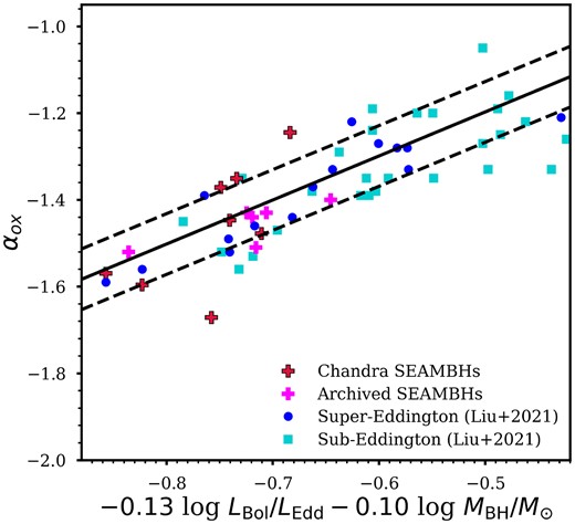
αox as a function of both |$\,\,\,\,\,\,\,\,{\dot{\mathscr {\!\!\!\!\!\! M}}}$| and MBH. The solid black line represents the best-fitting relation from Liu et al. (2021) and the dashed line represents the 0.07 scatter around it.
6 DISCUSSION AND CONCLUSIONS
One version of the disc–corona model assumes a thin Shakura & Sunyaev (1973) disc tightly coupled with a plane-parallel corona. The magnetic field in the accretion disc is produced by dynamo action, and the buoyancy of the magnetic fields generates magnetic loops that emerge into the corona. The loops reconnect with other loops, transferring the magnetic energy of the disc to thermal energy, thereby heating the corona. A stable corona is formed when the density of the corona reaches a certain value, allowing equilibrium between the heating by magnetic flux loops and cooling by Compton scattering. The coupling between the optical-UV emission from the accretion disc and the hard X-ray emission from the corona is often explained via such magnetic reconnection-heated model (Liu, Mineshige & Ohsuga 2003; Cao 2009). A fraction of gravitational energy is transferred from the accretion disc to the corona through magnetic fields that inhibit the fast cooling of the corona (Merloni & Fabian 2001). Magnetohydrodynamic simulations predict a decrease in the fraction of energy dissipated from the accretion disc as the disc transitions to radiation-pressure-dominated in case of higher accretion rate (higher LBol/LEdd)(Jiang, Stone & Davis 2014; Jiang et al. 2019). As a result, the corona becomes relatively more compact and weaker with an increasing Eddington ratio, resulting in a steeper αox. An increase in LBol/LEdd implies more soft photons from the accretion disc to cool the corona by Compton scattering, resulting in a steeper/softer Γ2-8 keV. In SEAMBHs, the inner accretion disc is perhaps geometrically thick, according to the slim disc model (Abramowicz et al. 1988; Laor & Netzer 1989; Wang & Zhou 1999; Wang et al. 2013), leading to differences in the accretion disc–corona connection. However, our analysis shows that the Γ2-8 keV–|$L_{\rm Bol}/L_{\rm Edd}(\,\,\,\,\,\,\,\,{\dot{\mathscr {\!\!\!\!\!\! M}}}$|) and αox–|$L_{\rm 2500 {\mathring{\rm A}}}$| (also L2 keV-|$L_{\rm 2500 {\mathring{\rm A}}}$|) relationships shows no dichotomy between the sub- and super-Eddington sources. This could mean that the transition from geometrically thin to a slim disc is not abrupt, and the disc–corona connection remains intact in super-Eddington AGNs. Another possibility is that there is no structural difference in the accretion disc of sub- and super-Eddington sources.
The correlations between X-ray properties and Eddington ratios studied in this paper are influenced by the choice of the bolometric correction used to estimate the bolometric luminosity. We used a correction factor of 9.26 to estimate the bolometric luminosity from |$L_{5100 {\mathring{\rm A}}}$|, consistent with literature values ranging between 7 and 13 (e.g. Elvis et al. 1994; Richards et al. 2006; Runnoe, Brotherton & Shang 2012, and references within). However, Jin, Ward & Done (2012) find the bolometric correction factor of 15 for their full sample and 20 for the sample of 12 narrow-line Seyfert 1 galaxies, using a colour temperature-corrected SED fitting model. Additionally, there are theoretical bolometric corrections based on the thin disc model that yield substantial differences, but they are inconsistent with empirically determined bolometric luminosities (e.g. Kubota & Done 2019).
We compared our bolometric luminosity measurements with those obtained through SED fitting by Liu et al. (2021) and the bolometric correction factor described in Netzer (2019). Liu et al. (2021) derived bolometric luminosities by integrating the infrared-to-X-ray SED (see their section 2.7 for details). For the three AGNs in our Chandra sample, i.e. IRAS04416+1215, SDSSJ074352.02+271239.5, SDSSJ100402.61+285535.3, the differences in the logarithm of bolometric luminosity measured by Liu et al. (2021) compared to our method are 0.083, −0.017, and −0.147, respectively. Notably, we found a higher level of agreement for the super-Eddington sample, with a median difference of 0.183, ranging between −0.197 and 0.413. In contrast, the median difference for the sub-Eddington sample was 0.25, ranging from −0.187 to 0.683. It is important to emphasize that the determination of bolometric luminosities through multiwavelength SEDs may have considerable uncertainties, especially for super-Eddington accreting quasars. This is due to various factors such as host-galaxy contamination and variability effects due to non-simultaneous SED data. Furthermore, super-Eddington accreting quasars may have significantly enhanced EUV emission compared to typical quasars, but there is no clear observational constraint on this due to the lack of data (Jin, Ward & Done 2012; Castelló-Mor, Netzer & Kaspi 2016; Kubota & Done 2019). Next, we test our choice of bolometric correction against the correction factor given in Netzer (2019). Instead of a constant of 9.26, the Netzer (2019) bolometric correction factor is a function of monochromatic luminosity at |$5100{\mathring{\rm A}}$| and is expressed as |$40~ [L_{\rm 5100{\mathring{\rm A}}} (\rm observed)/10^{42} \rm erg ~ s^{-1}]^{-0.2}$|. The two sets of estimates give very similar values. The agreement is slightly better for the sub-Eddington sample, with the median value of logarithmic difference being −0.0016, while it is −0.0576 for the super-Eddington sample.
Our choice of bolometric correction is conservative and does not make any enhancement in the bolometric luminosity, hence Eddington ratio, preferentially for the SEAMBHs even though that may be the case (Jin, Ward & Done 2012).
One of our targets, SDSS J101000.68+300321.5, exhibits a flatter/harder Γ2-8 keV and appears as X-ray-weak (Δαox < −0.2). It could be that the X-ray data for this object are not good enough, as indicated by large error bars, or the possibility that the X-ray emission is shielded by a puffed-up slim accretion disc. Luo et al. (2015) explain X-ray weakness in highly accreting AGNs through an orientation effect in a slim accretion disc. When viewed at larger inclination angles, X-rays emitted from the central region may be absorbed by the puffed-up inner accretion disc (Luo et al. 2015; Ni et al. 2018). Liu et al. (2019) estimate that 15–24 per cent of super-Eddington AGNs should exhibit extreme X-ray variability. Our comparison sample from Liu et al. (2021) selectively chooses the high X-ray state for the sub- and super-Eddington samples with multiple X-ray observations, thereby excluding any X-ray-weak object from the sample. One recent X-ray spectroscopic study of highly accreting AGNs by Laurenti et al. (2022) reports 29 per cent of the sample as X-ray-weak. A dramatic change in X-ray flux is seen in some weak emission-line quasars with high accretion rates whose X-ray variability can be explained due to changes in the thickness of the accretion disc (Liu et al. 2019; Ni et al. 2020). Our target SDSS J101000.68+300321.5 could be an X-ray-weak weak-emission line quasar that has weak high-ionization lines like C iv|$\rm \lambda 1549$|. The lack of UV spectra for this target inhibits us from testing this hypothesis. Alternatively, the X-ray weakness may be caused by absorption from outflows, which also manifest UV absorption troughs in some AGNs (e.g. Kaastra et al. 2014, and references therein).
It is worth noting that the extreme SEAMBHs studied in this paper are primarily narrow-line Seyfert 1 galaxies (NLS1s). NLS1s are believed to be accreting material at rates approaching the Eddington limit, as supported by various studies (Komossa et al. 2006; Peterson 2011; Komossa 2018; Peterson & Dalla Bontà 2018; Foschini 2020). The optical spectra of NLS1s are characterized by several distinctive features, such as relatively narrow H β emission lines, strong Fe ii lines, and weak [O iii] lines (Boroson 2002). These characteristics align with the Eigenvector 1 trends, known to correlate with accretion rate (Boroson & Green 1992; Marziani et al. 2001; Boroson 2002; Yuan & Wills 2003; Shen & Ho 2014; Sun & Shen 2015). In X-rays, NLS1s exhibit steep 2–10 keV spectra and a pronounced soft X-ray excess (e.g. Boller, Brandt & Fink 1996; Brandt, Mathur & Elvis 1997; Véron-Cetty, Véron & Gonçalves 2001). The question arises: is the steepness of the 2–8 keV X-ray spectrum solely due to the extreme accretion rate, or can it be attributed to factors like coronal geometry or distinct cooling mechanisms within the corona specific to NLS1s? This intriguing question presents a potential avenue for future investigations using broad-band X-ray spectra. Recent research has shown a certain subjectivity in these classifications. For instance, Jin et al. (2023) indicated a connection between NLS1s with extreme accretion rates and weak-line quasars (WLQs). Additionally, Ha et al. (2023) demonstrated that WLQs follow the same trend of C iv versus Eddington ratio as other type-1 quasars.
In conclusion, we present new Chandra X-ray data of nine SEAMBHs. Our core sample consists of 14 SEAMBHs that have extremely high accretion rates (|${\rm log}~ \,\,\,\,\,\,\,\,{\dot{\mathscr {\!\!\!\!\!\! M}}}\gt 1.5$|) and show the largest offset between the radius of BLR from the RM measurement and the one estimated from the canonical R–L relationship. We investigated the X-ray and optical-UV properties of these 14 extreme SEAMBHs and compared them to the sub- and super-Eddington quasars from Liu et al. (2021). To mitigate errors due to variability, we took almost simultaneous X-ray and optical-UV observations for the Chandra SEAMBHs. However, it should be noted that there is an intrinsic delay between the X-ray and the optical-UV variability due to the spatial difference in the regions emitting these radiations. We used Du & Wang (2019) for the black hole properties. Our results indicate that extreme SEAMBHs indeed have a steep 2–8 keV X-ray photon index and demonstrate a steeper power-law slope. They are consistent with a correlation between Γ2-8 keV and LBol/LEdd (also |$\,\,\,\,\,\,\,\,{\dot{\mathscr {\!\!\!\!\!\! M}}}$|) seen in sub- and super-Eddington accreting sources. We show that the αox–|$L_{\rm 2500 {\mathring{\rm A}}}$| (also L2 keV–|$L_{\rm 2500 {\mathring{\rm A}}}$|) correlation extends to the extreme SEAMBHs. The αox–|$\,\,\,\,\,\,\,\,{\dot{\mathscr {\!\!\!\!\!\! M}}}$| correlation remains weak after the inclusion of eight extreme SEAMBHs; however, the bivariate relationship established by Liu et al. (2021) between αox, LBol/LEdd, and MBH holds for the extreme SEAMBHs.
ACKNOWLEDGEMENTS
We express our gratitude to the anonymous referee for providing constructive comments that enhanced the quality of the manuscript. We acknowledge support through Chandra Award Number GO9-20107X. BL acknowledges financial support from the National Natural Science Foundation of China grant 11991053. This research has used data obtained from the Chandra Data Archive and the Chandra Source Catalog, and software provided by the Chandra X-ray Center (CXC) in the application packages ciao and sherpa. This research has used the NASA/IPAC Extragalactic Database (NED), which is operated by the Jet Propulsion Laboratory, California Institute of Technology, under contract with the National Aeronautics and Space Administration.
DATA AVAILABILITY
The Chandra data used in this paper can be downloaded from the Chandra Data Archive (PI: Brotherton; PI: Garmire). Section 3 provides detail of the data analysis and Tables 1, 2, 3, and 4 list all the measured quantities for Chandra SEAMBHs and one Archived SEAMBH. The data for other Archived SEAMBHs, super- and sub-Eddington are available in Liu et al. (2021) (DOI: 10.3847/1538-4357/abe37f).
References
APPENDIX A:
This paper analysed the Chandra data of four SEAMBHs that are previously studied. Here, we compare our results with the literature values, focusing mostly on the 2–8 keV photon index as our study is based on it. We find that our measurements are consistent with the literature values.
IRAS 04416+1215: Liu et al. (2021) find a photon index of |$2.46_{-026}^{+0.27}$| in the |$\gt 2~ \rm keV$|Swift spectrum. A broad-band XMM–Newton and NuSTAR study by Tortosa et al. (2022) reveals that the reflected radiation dominates the primary continuum, which exhibits a slope of 1.77.
SDSS J074352.02+271239.5: The 2–8 keV photon index |$2.06^{+0.31}_{-0.30}$| was measured by Liu et al. (2021) using Swift data.
SDSS J100402.61+285535.3: Analysis of XMM–Newton data by Liu et al. (2021) shows a >2 keV photon index of 2.31 ± 0.05, which is consistent with our measurement given the uncertainty.
SDSSJ075051.72+245409.3: Huang et al. (2023) find the 0.3–8 keV photon index of 2.22 ± 0.19 using Chandra data. Our 0.35–8 keV measurement is consistent with their findings.
