


ABSTRACT
The full-disc chromosphere was routinely monitored in the He i 10 830 Å line at the National Solar Observatory/Kitt Peak from 2004 November to 2013 March, and thereby, synoptic maps of He i line intensity from Carrington rotations 2032 to 2135 were acquired. They are utilized to investigate the differential rotation of the chromosphere and the quiet chromosphere during the one falling (descending part of solar cycle 23) period and the one rising (ascending part of solar cycle 24) period of a solar cycle. Both the quiet chromosphere and the chromosphere are found to rotate slower and have a more prominent differential rotation in the rising period of solar cycle 24 than in the falling period of solar cycle 23, and an illustration is offered.
1 INTRODUCTION
The solar atmosphere is magnetic, and the magnetic field is the main source of solar activities and changes (Xiang, Qu & Zhai 2014; Xiang, Ning & Li 2020; Li, Xu & Feng 2022). The differential rotation of the solar atmosphere has always been an important field in solar physics and has been widely investigated due to its intimate relationship to the solar magnetic field through the solar dynamo (Beck 2000; Thompson et al. 2003). The entire solar atmosphere, from the bottom photosphere layer to the top corona layer, has been known to differentially rotate; that is, its rotation rate is the largest at the equator and decreases with increasing of latitudes, perhaps due to the effect of the Coriolis force exerted by the rotational motion on the convective motion (Howard 1984; Chandra, Vats & Iyer 2009, 2010; Wöhl et al. 2010; Vats & Chandra 2011a, b; Gigolashvili, Japaridze & Kukhianidze 2013; Hiremath & Hegde 2013; Javaraiah 2013, 2020; Shi & Xie 2013; Sudar et al. 2014, 2015; Javaraiah & Bertello 2016; Obridko & Shelting 2016; Badalyan & Obridko 2017; Bhatt et al. 2017; Ruždjak et al. 2017; Xie, Shi & Zhang 2017; Deng et al. 2020; Mierla et al. 2020; Singh et al. 2021a, b; Edwards et al. 2022; Poljančić Beljan et al. 2022). The helioseismic measurements of the inner zonal and meridional flows are the foundation for understanding the differential rotation of the solar atmosphere and its relationship with the magnetic fields and the solar dynamo (Howe 2009; Komm et al. 2009).
In the photosphere, the rotation rate of plasma determined by spectroscopic measurements is consistently lower than that of sunspots determined by tracer measurements, and small sunspots rotate slightly faster than big ones in general (Snodgrass, Howard & Webster 1984; Jha et al. 2021; Kutsenko 2021). One reasonable speculation for these results is that sunspots of different sizes are rooted at different depths (Beck 2000; Wan et al. 2023). Large-size sunspots are found to repress the differential of rotation in the photosphere (Brajša et al. 1996; Brajša, Ruždjak & Wöhl 2006; Jurdana-Šepić et al. 2011; Li et al. 2020; Wan & Gao 2022). One plausible explanation for this result is that appearance of sunspots at low latitudes (10°–35°) should upraise the rotation profile of photosphere plasma at the latitudes, due to that sunspots rotate faster than the photosphere plasma (Li et al. 2020).
In the chromosphere, short-lived features observed in the Ca ii K line rotate at the same velocity as the chromospheric plasma (Antonucci et al. 1979a, b; Xu, Xie & Qu 2019; Xu, Gao & Shi 2020), which actually means that small-size magnetic elements rotate at the same rate as the quiet (background) chromosphere, in agreement with Li et al. (2020, 2022). The heating and formation of the quiet chromosphere are believed to be caused mainly by the small-scale magnetic elements whose magnetic flux is in range of (2.9–32.0) × 1018 Mx, because the long-term evolution of the quiet chromosphere (intensity values at its full surface) is found to be in antiphase with the solar cycle (Li & Feng 2022; Li et al. 2022), as the long-term evolution of the small-scale magnetic elements does (Jin et al. 2011; Jin & Wang 2012). We note that in this context, ‘antiphase’ refers to two variables behaving in an opposite manner such that one reaches its peak, the other is at its minimum, and vice versa. Therefore, the quiet chromosphere rotates at the same rate as the small-scale magnetic elements do (Li et al. 2020; Li, Wan & Feng 2023). It is speculated that the small-scale magnetic elements come from the leptocline (Lefebvre, Nghiem & Turck-Chieze 2009), and it rotates clearly faster than the surface (photosphere) rotation (Larson & Schou 2018). Therefore, the quiet chromosphere and the chromosphere rotate clearly faster than the photosphere. The quiet chromosphere is found to rotate faster than sunspots at relatively high latitudes of the butterfly pattern of sunspots, but slower at lower latitudes (Li et al. 2020, 2023; Wan & Gao 2022; Wan et al. 2023), and thus the chromosphere rotates a bit faster than the quiet chromosphere at lower latitudes, but slightly slower at relatively high latitudes of the butterfly pattern. Therefore, the level of the differentiality of the rotation of the chromosphere is higher than that of the quiet chromosphere; that is, the large-scale magnetic fields strengthen the differential in the chromosphere. The level of the differentiality of rotation is in order from smallest to largest: the quiet chromosphere, the quiet photosphere, the chromosphere, and sunspots (Li et al. 2023).
The corona is more dynamic than the underlying chromosphere and photosphere, and thus it is difficult to continue for one rotation period or more to track coronal features. Therefore, the results obtained by different methods for coronal rotations of different features at different time intervals are sometimes mixed, and in particular the results for the differential in coronal rotations are even contradictory to some extent. Nevertheless, some consensus has been reached. Like the chromosphere, the corona rotates faster and less differentially than the photosphere (Mancuso & Giordano 2011; Mancuso et al. 2020; Sharma et al. 2021, 2023).
The relationship between the rotation of the photosphere and solar activity or the solar cycle is an interesting topic and has been widely studied (Balthasar & Wöhl 1980; Obridko & Shelting 2001; Jurdana-Šepić et al. 2011; Javaraiah 2013; Poljančić Beljan et al. 2022; Wan & Gao 2022; Wan et al. 2023). In the photosphere, the torsional oscillation (TO) is the most prominent feature of the rotation of the atmosphere (plasma), and the high-speed zone of the TO pattern basically coincides with the zone of sunspots’ appearance (Howard & LaBonte 1980; Li et al. 2008). Although both the zones individually exhibit the characteristics of the activity cycle, there may be complex links found between the rotation of the photosphere and solar activity or the solar cycle in practical studies (Brajša et al. 2006; Lekshmi, Nandy & Antia 2018), due to the following factors. First of all, the rotation rate of the photosphere averaged over latitudes at a certain time varies with the range and number of latitudes considered; that is, there is not an exact value of the differential rotation rate averaged over latitudes at a certain moment. Some parameters, such as the equatorial rotation rate and the differential of rotation (the latitudinal gradient of rotation), have more suitable practicability to describe the differential rotation than the rotation rate does. Secondly, in general in the photosphere, large-scale magnetic fields suppress the differential of rotation rates, while small-scale magnetic fields (SMFs) seemingly reflect the differential of rotation rates (Li et al. 2013a; Li, Xie & Shi 2013b), and thus sunspots of large and small scales may appear at different times and latitudes within a solar cycle, exerting different effects on the rotation of the photosphere. In the chromosphere layer, SMFs, which cause the rotation of the quiet chromosphere to be the same as their own rotation (Li et al. 2022, 2023), are in antiphase with the solar cycle (Jin et al. 2011; Jin & Wang 2012), but the differential of rotation in the quiet chromosphere is recently found to have no relation with the solar cycle (Wan et al. 2023). The differential of rotation in the chromosphere is, however, found to have a significantly negative relation with the solar cycle, due to the enhancement effect of large-scale magnetic fields on the differential of rotation (Wan & Gao 2022). During the maximum epoch of a solar cycle, there are more large-scale magnetic fields and stronger enhancement effects, and thus the differential of rotation is smaller (its absolute value is larger). In the corona layer, the rotation of the atmosphere (structures) is found to be multifariously related with solar activity or the solar cycle (Vats et al. 1998; Jurdana-Šepić et al. 2011; Sharma et al. 2023). Before understanding the relationship of coronal rotations and the magnetic fields, we need to investigate the relation between the formation of the corona and the magnetic fields (Li et al. 2022).
The chromosphere was routinely monitored in the He i 10 830 Å absorption line at the National Solar Observatory/Kitt Peak from 2004 November to 2013 March, and synoptic maps in the time interval are acquired. Li et al. (2020) once investigated the differential rotation of the chromosphere by means of the data. In this study, the entire data of more than 8 years will be divided into two parts, the descending part of the solar cycle 23 and the ascending part of the solar cycle 24, and then the differential rotation in different phases of a solar cycle will be investigated.
2 DATA AND METHODS
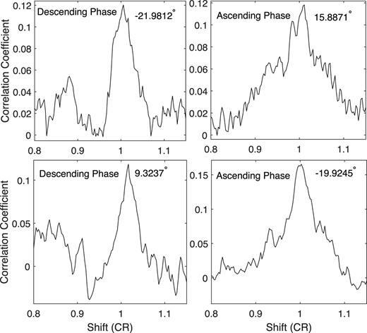
Data used in this study are synoptic maps of He i line intensity from Carrington rotations 2032 to 2135, which came from daily observations of the full-disc chromosphere in the He i 10 830 Å line at the National Solar Observatory/Kitt Peak (Livingston et al. 1976; Harvey & Livingston 1994), in the time interval of 2004 November (later than the maximum time of cycle 23, 2000 July) to 2013 March (earlier than the maximum epoch of cycle 24, 2014 February). In all, the data cover 104 synoptic maps. Each synoptic map was gauged across 360 equidistant longitudes that span from 1° to 360° and 180 latitudes. The latitudinal measurements took 180 uniform steps based on the sine of the latitude, extending from −1 (the south pole) to +1 (the north pole). By compiling all the 104 synoptic maps chronologically, we achieved one seamless synoptic image. The intensity of the He i line is in arbitrary but constant unit. Fig. 1 shows the data just within latitudes not higher than 30°. Details of the data may be found in Li et al. (2020). In order to determine the periodicity of a time series, the autocorrelation analysis method will be utilized in the following analyses [for details, please refer to Xu & Gao (2016)], and this method was once used to determine the rotation period of the entire data length by Li et al. (2020), but here the data are divided into two parts. The minimum epoch of cycle 24 is December 2008 (Carrington rotation 2077), and then accordingly, the first part includes Carrington rotations 2032 to 2076, belonging to the descending phase of cycle 23, and the second is the synoptic images of Carrington rotations 2077 to 2135, belonging to the ascending phase of cycle 24. Here, we take the same processing procedure as Li et al. (2020) did, but the entire data used by Li et al. (2020) are replaced, respectively, by the two parts. Resultantly as examples, Fig. 2 shows correlation coefficient of a time series versus itself, varying with their relative phase shifts, in each of the total four panels, and two panels in the figure show the calculated results of time series in the ascending phase, while the other two show those of time series in the descending phase. In the figure, CR means the synodic Carrington rotation period, and 1CR = 27.2753 d. When the synodic rotation period (SRP) of a series at a measurement latitude is determined, the rotation velocity at the latitude can be known: SRP × 360/27.2753 ≈ 13.1988SRP (in degrees/day; Li et al. 2020). Finally, synodic rotation velocities at all measurement latitudes that are not higher than 30° are determined, which are shown in Fig. 3, and meanwhile the correlation coefficient corresponding to the SRP at a measurement latitude is also displayed in the figure, which is statistically significant at the |$99{{\ \rm per\ cent}}$| confidence level.
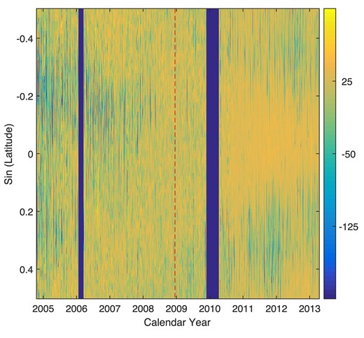
Synoptic images (time–latitude diagram) of He i intensity in the interval of 2004 November to 2013 March, but only latitudes not higher than 30° are displayed here. The colour bar indicates the intensity of the He i line with an arbitrary but constant unit. The two vertical blue bands indicate no observational data available, and the red dashed line shows the minimum time of cycle 24.
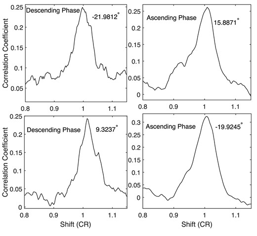
Correlation coefficient of a time series of He i line intensity at a certain latitude versus itself, varying with their relative phase shifts. Four panels correspond to four time series, whose latitudes are displayed in the upper right corner of each panel. In a panel, the words ‘Ascending Phase’ mean that a time series of He i line intensity in the ascending phase of solar cycle 23 is used to determine the rotation period of the series, while the words ‘Descending Phase’ mean that a time series of He i line intensity in the descending phase of solar cycle 24 is used.
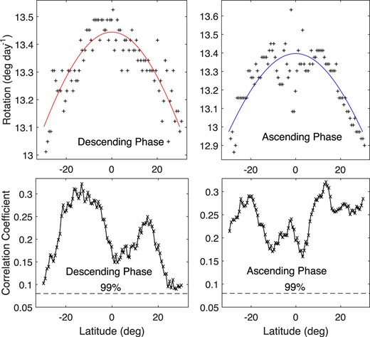
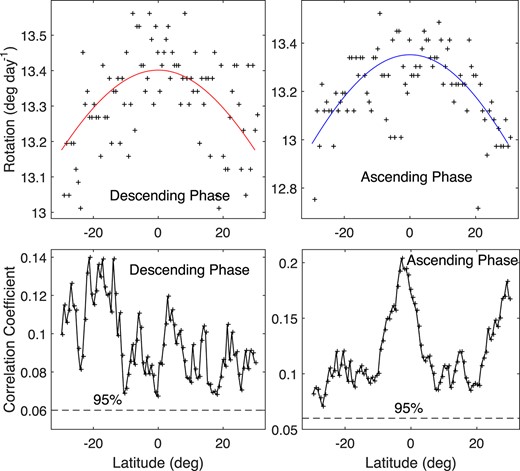
Synodic rotation velocities (pluses, top panels) and their corresponding correlation coefficients (crosses in a black solid line, bottom panels) at measurement latitudes that are not higher than 30°, determined, respectively, in the descending phase (left panels) and the ascending phase (right panels). The solid lines are the fitting lines of synodic rotation velocities, respectively, in the descending and ascending phases, and the dashed lines show the |$99{{\ \rm per\ cent}}$| confidence level.
3 DIFFERENTIAL ROTATION OF THE CHROMOSPHERE
At low latitudes (φ) not higher than 30°, the following theoretical expression is usually utilized to fit observational velocities (ω) of the differential rotation:
where the undetermined parameter A is the rotation velocity at the solar equator, and the undetermined parameter B reflects the differential degree of rotation. Here, the expression is utilized to fit observational rotation velocities, and the bootstrap method (Xu et al. 2019) is used to determine values of the undetermined parameters (A and B) and their errors. The differential rotation of the He i chromosphere in the descending phase of cycle 23 is determined to be
and that in the ascending phase of cycle 24,
The parameters A and B in the descending phase are different from those in the ascending phase. Specifically in the descending phase, the rotation at the equator is faster, but differential degree is lower, than that in the ascending phase.
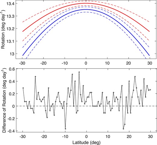
These two fitting lines are put together and shown in Fig. 4. The difference of rotation velocity at a measurement latitude, respectively, in the descending and ascending phases is also displayed in the figure. Of the 90 measurement latitudes, rotation velocity determined in the descending phase is equal to that in the ascending phase at 13 latitudes, larger at 57 latitudes, and smaller at 20 latitudes. The Wilcoxon test method for paired observations (Hollander & Wolfe 1973) is utilized to examine statistical significance of the difference between these two velocity distributions. The calculated Z-value for the + sign is 4.22, which is larger than the tabulated critical value (2.58) at the 0.01 significance level. Fig. 4 also shows the error (1σ) lines of these two fitting lines, and the difference between the fitting lines is significant at the 1σ level (Brajša et al. 1995, 1999). Therefore, generally, the rotation velocity in the descending phase is greater than that in the ascending phase.
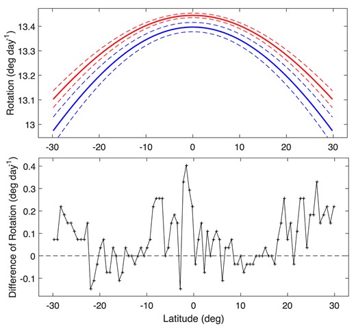
Top panel: the fitting line of synodic rotation velocities respectively in the descending phase of cycle 23 (the top solid thick line) and the ascending phase of cycle 24 (the bottom solid thick line). The top (bottom) dashed thin line is the error line of the top (bottom) solid thick line. Bottom panel: difference (crosses) of the value respectively in the top and bottom lines at a measurement latitude.
4 DIFFERENTIAL ROTATION OF THE QUIET CHROMOSPHERE
Those intensities not less than −10 can be approximated as coming from the quiet chromosphere (Li et al. 2020). Note that the He i line intensity in synoptic maps is represented in arbitrary but constant unit. Therefore, in order to investigate the differential rotation of the quiet chromosphere, it is them that are considered in the following analysis. We repeat the above analysis, but intensities in the chromosphere are replaced by those in the quiet chromosphere. Here, as four examples, Fig. 5 shows four calculated correlation-coefficient profiles at the same latitudes as Fig. 2, and Fig. 6 is similar to Fig. 3, showing the determined synodic rotation velocities and the corresponding correlation coefficients. These coefficients are significant at the |$95{{\ \rm per\ cent}}$| confidence level. The expression is also utilized to fit observational rotation velocities, and the differential rotation of the quiet chromosphere in the descending phase is
and that in the ascending phase,
For the quiet chromosphere, the rotation at the equator is faster, but differential degree is lower, in the descending phase than in the ascending phase.
The same as Fig. 2, but just those intensities that are not less than −10 are considered; that is, the quiet chromosphere is considered instead of the chromosphere.
The same as Fig. 3, but just those intensities that are not less than –10 are considered; that is, the quiet chromosphere is considered instead of the chromosphere.
These two fitting lines and their error lines are shown together in Fig. 7, and displayed also in the figure is the difference of rotation velocity, respectively, in the descending and ascending phases. Rotation velocity in the descending phase is larger at 61 latitudes and smaller at 21 latitudes than that in the ascending phase. Similarly, the Wilcoxon test method (Hollander & Wolfe 1973) is utilized to examine statistical significance of the difference between these two velocity distributions. The calculated Z-value for the + sign is 4.41, which is larger than the critical value (2.58) at the 0.01 significance level. As the figure displays, the difference between the fitting lines is significant at the 1σ level (Brajša et al. 1995, 1999). Therefore, in the quiet chromosphere, the rotation velocity in the descending phase is generally greater than that in the ascending phase.
The same as Fig. 4, but just those intensities that are not less than −10 are considered; that is, the quiet chromosphere is considered instead of the chromosphere.
5 COMPARISON OF THE DIFFERENTIAL ROTATION OF THE CHROMOSPHERE AND THE QUIET CHROMOSPHERE
The two fitting lines in the descending phase, corresponding to the differential rotation of the chromosphere and that of the quiet chromosphere, are displayed together in the top panel of Fig. 8, and the fitting lines in the ascending phase are displayed together in the bottom panel of the figure. The differential rotation of sunspots is generally adopted the expression (Howard 1996; Komm et al. 2009):
for the synodic rotation, and it is also plotted in the figure. The commonly used expression for the differential rotation of the photosphere is (Snodgrass et al. 1984; Komm et al. 2009):
for the synodic rotation, and it is drawn in the figure as well. As the figure indicates, (1) the chromosphere and the quiet chromosphere rotate clearly faster than the photosphere; (2) the chromosphere rotates faster than the quiet chromosphere at much low latitudes (less than about 20°), but slower at middle latitudes; and (3) sunspots rotate faster than the chromosphere and the quiet chromosphere at much low latitudes (less than about 15°), but slower at latitudes higher than about 18°.
![Top panel: the fitting line of the differential rotation in the descending phase of cycle 23, respectively, for the chromosphere (the thin red line) and the quiet chromosphere (the thin blue line) from this work. Bottom panel: the fitting line of the differential rotation in the ascending phase of cycle 24, respectively, for the chromosphere (the thin red line) and the quiet chromosphere (the thin blue line) from this work. In both panels, the thick red line displays the differential rotation of the photosphere [adopted from Snodgrass et al. (1984) and Komm et al. (2009)], while the differential rotation of sunspots is shown by the thick blue line [adopted from Howard (1996) and Komm et al. (2009)].](https://oup.silverchair-cdn.com/oup/backfile/Content_public/Journal/mnras/528/2/10.1093_mnras_stae044/1/m_stae044fig8.jpeg?Expires=1749298200&Signature=H3eybFTc90V3-TrCVJ71deqZRVDyJLdiFOxe8oYrGznyHUf7XZlTNEnEnmwBuaQxS0aatSQhxVij6wEquTj80DJ18eEzOqhEp3xdBEpQ9Rnj6RI7bYJ65WQyrvDcH94YwAoNF7tKVdqGCdJtkEdOJuKXZTlCJvWbl3-ckgkdk7td-I7Yk12ADHvjS~gKbbKxcN~bQZNYOsyqbM5MDPK7PhxAoFSgw6mywbZASIj3RIyDDGcukH-iOfYn~tdpr9w-SiJSTsrdXDupAYi86yRnOrDMVqGTMKlu-yaxvcT5pbHyg02wnufWx-c2xwpzArGFy3~UuX6u4vHPu~xwr-AO4A__&Key-Pair-Id=APKAIE5G5CRDK6RD3PGA)
Top panel: the fitting line of the differential rotation in the descending phase of cycle 23, respectively, for the chromosphere (the thin red line) and the quiet chromosphere (the thin blue line) from this work. Bottom panel: the fitting line of the differential rotation in the ascending phase of cycle 24, respectively, for the chromosphere (the thin red line) and the quiet chromosphere (the thin blue line) from this work. In both panels, the thick red line displays the differential rotation of the photosphere [adopted from Snodgrass et al. (1984) and Komm et al. (2009)], while the differential rotation of sunspots is shown by the thick blue line [adopted from Howard (1996) and Komm et al. (2009)].
Here, a classical relation between synodic (ωsyn) and sidereal ωsid rotation velocities is used (Brajša et al. 1999; Skokić et al. 2014): ωsyn = ωsid − 0.9856 (deg d−1), and it is convenient for us to investigate the differential rotation of the chromosphere and the quiet chromosphere during the one falling and one rising periods of a solar cycle. Of course, a precise transformation should refer to Skokić et al. (2014), due to the Earth’s ellipticity orbit and temporal variation of solar rotation axis to the ecliptic (Graf 1974; Roša et al. 1995; Brajša et al. 2002).
6 CONCLUSIONS AND DISCUSSION
In this study, the synoptic images of He i 10 830 Å line intensity from Carrington rotations 2032 to 2135 are used to explore the differential rotation of both the chromosphere and the quiet chromosphere, respectively, during the ascending and descending phases of a solar cycle, and some interesting results are obtained. We note that although we speculate our results should also be applicable to other cycles, the limitations of the available data necessitate more extensive analysis for a definitive generalization.
Based on this study and Li et al. (2020), the following results hold true whether in the rising period, the falling period of a solar cycle, or a solar cycle. The differential rotation of both the chromosphere and the quiet chromosphere is significantly greater than that of the photosphere; the quiet chromosphere rotates slightly slower than the chromosphere at lower latitudes around the equator, but a little faster at latitudes higher than ∼20°; and sunspots rotate a bit faster than the chromosphere and the quiet chromosphere at latitudes lower than ∼15°, but explicitly slower at latitudes higher than ∼18°. These results were reasonably explained by Li et al. (2020). It is mainly the SMFs whose magnetic flux is in the range of (2.9–32.0) × 1018 Mx (Jin et al. 2011; Jin & Wang 2012) that make the rotation of the quiet chromosphere different from that of the photosphere, and then further, sunspots make the rotation of the quiet chromosphere different from that of the chromosphere; therefore, the quiet chromosphere and SMFs are both in antiphase with the solar cycle (Li & Feng 2022; Li et al. 2022, 2023).
The quiet chromosphere is found to rotate faster in the falling period than in the rising period of a solar cycle, but its differential degree of rotation is smaller in the falling period than in the rising period. Jin & Wang (2012) gave time–latitude distribution of peak values of the probability distribution functions of latitude for SMFs (the anticorrelated network elements) in their fig. 5. The figure indicates that SMFs are mainly distributed at latitudes higher than ∼20° in the falling period of a solar cycle and at latitudes lower than ∼20° in the rising period. The rotation velocity of SMFs is greater than that of the photosphere (Xu et al. 2016; Li et al. 2020).
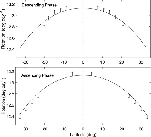
It is assumed that the rotation of the quiet chromosphere is caused by the action of SMFs on the rotation of the photosphere (Li et al. 2022), and then the action of SMFs on the rotation of the photosphere, respectively, in the falling and rising periods is illustrated in Fig. 9, based on the time–latitude distribution. In the falling period, SMFs emerge and act on the rotation of the photosphere from latitudes higher than ∼20°, and thus they increase rotation velocities but attenuate the rotation differential of the photosphere. In the rising period, SMFs emerge and act on the rotation of the photosphere from the latitudes lower than ∼20°, and thus they increase rotation velocities and strengthen the rotation differential of the photosphere. This is why the differential degree of rotation in the quiet chromosphere is smaller in the falling period than in the rising period. As for that the quiet chromosphere rotates faster in the falling period than in the rising period of a solar cycle, perhaps it is because more SMFs appear in the falling period.
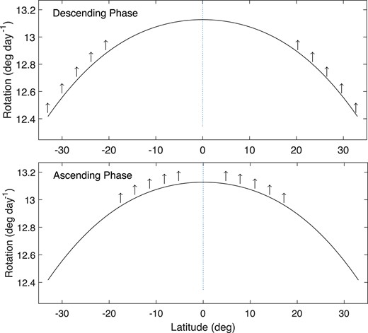
Schematic diagram of the effect (up arrows) of SMFs on the differential rotation of the photosphere (the solid line), respectively, in the descending (the top panel) and ascending (the bottom panel) phases. Up arrows mean that SMFs increase the rotation velocity of the photosphere.
Recently, the quiet chromosphere is found to rotate a litter faster than sunspots at relatively high latitudes of the butterfly diagram of sunspots, but a bit slower at low latitudes round the equator (Li et al. 2020, 2023). In the falling period of a solar cycle, sunspots are known to generally appear at lower latitudes of the butterfly pattern, and in the rising period sunspots appear at higher latitudes of the butterfly pattern and low latitudes around the equator, for that some small sunspots of the previous cycle may still appear at low latitudes when a new active cycle begins. It is assumed that the rotation of the chromosphere is caused by the action of sunspots on the rotation of the quiet photosphere, and then the action of sunspots on the rotation of the quiet chromosphere, respectively, in the falling and rising periods is illustrated in Fig. 10. In the falling period, sunspots emerge from lower latitudes of the butterfly pattern and act on the rotation of the quiet chromosphere, and thus they increase rotation velocity and strengthen rotation differential of the quiet chromosphere in general. In the rising period, sunspots emerge from higher latitudes of the butterfly pattern and low latitudes around the equator and act on the rotation of the quiet chromosphere, and thus they decrease rotation velocities and strengthen the rotation differential of the quiet chromosphere. This is why rotation velocity in the chromosphere is larger in the falling period than in the rising period. As for that the rotation differential degree of the chromosphere is lower in the falling period than in the rising period of a solar cycle, perhaps it is because the rotation differential degree of the quiet chromosphere is lower in the falling period. Of course in the rising and falling periods, different degree of sunspot action on the quiet chromosphere may also lead to difference of the chromospheric differential, and the difference is considered minor.
Schematic diagram of the effect (up or down arrows) of sunspots on the differential rotation of the quiet chromosphere (the solid line), respectively, in the descending (the top panel) and ascending (the bottom panel) phases. Up arrows mean that sunspots increase the rotation velocity of the quiet chromosphere and down arrows mean that sunspots decrease the rotation velocity.
Of course, we need to make it clear that our conclusion is derived using only one rising and falling period of the solar cycle, and thus more rising and falling periods are needed to generalize the conclusion in future.
To sum up, the quiet chromosphere and the chromosphere rotate faster, and the differential degree of their rotation is lower, in the falling period than in the rising period of a solar cycle, due to the effect of the magnetic fields on rotation.
ACKNOWLEDGEMENTS
We thank the anonymous referee very much for careful reading of the manuscript and constructive comments that significantly improved the original version of the manuscript. This work was supported by Yunnan Fundamental Research Project (202201AS070042 and 202101AT070063), the National Natural Science Foundation of China (12373059, 12373061, 11973085, and 41964007), the Yunling-Scholar Project (the Yunnan Ten-Thousand Talents Plan), the national project for large-scale scientific facilities (2019YFA0405001), the ‘Yunnan Revitalization Talent Support Program’ Innovation Team Project, the project supported by the specialized research fund for state key laboratories, and the Chinese Academy of Sciences.
DATA AVAILABILITY
Synoptic maps of intensity of the He i 10 830 Å line from Carrington rotations 2032 to 2135 come from the routine observations of the full-disc chromosphere in the line at the National Solar Observatory (NSO)/Kitt Peak. They are publicly available from the NSO’s web site, ftp://nispdata.nso.edu/kpvt/synoptic/.
