


ABSTRACT
Closely packed multiplanet systems are known to experience dynamical instability if the spacings between the planets are too small. Such instability can be tempered by the frictional forces acting on the planets from gaseous discs. A similar situation applies to stellar-mass black holes embedded in active galactic nuclei discs around supermassive black holes. We use N-body integrations to evaluate how the frictional damping of orbital eccentricity affects the growth of dynamical instability for a wide range of K (the difference in the planetary semimajor axes in units of the mutual Hill radius) and (unequal) planet masses. We find that, in general, the stable region (large K) and unstable region (small K) are separated by a “grey zone”, where the (in)stability is not guaranteed. We report the numerical values of the critical spacing for stability Kcrit and the “grey zone” range in different systems, and provide fitting formulae for arbitrary frictional forcing strength. We show that the stability of a system depends on the damping time-scale τ relative to the zero-friction instability growth time-scale tinst: two-planet systems are stable if tinst ≳ τ; three-planet systems require tinst ≳ 10τ−100τ. When K is sufficiently small, tinst can be less than the synodic period between the planets, which makes frictional stabilization unlikely to occur. As K increases, tinst tends to grow exponentially, but can also fluctuate by a few orders of magnitude. We also devise a linear map to analyse the dynamical instability of the “planet + test mass” system, and find qualitative agreement with N-body simulations.
1 INTRODUCTION
Planetary systems with two or more planets can be dynamically unstable if the spacing between the planetary orbits is small (e.g. Wisdom 1980; Gladman 1993; Chambers, Wetherill & Boss 1996; Zhou, Lin & Sun 2007; Smith & Lissauer 2009; Funk et al. 2010; Deck, Payne & Holman 2013; Pu & Wu 2015). This instability typically results in collisions or strong scatterings between the planets, which have significant impacts on the architecture of the planetary systems (e.g. Rasio & Ford 1996; Weidenschilling & Marzari 1996; Lin & Ida 1997; Ford, Havlickova & Rasio 2001; Adams & Laughlin 2003; Nagasawa & Ida 2011; Petrovich, Tremaine & Rafikov 2014; Frelikh et al. 2019; Anderson, Lai & Pu 2020; Li & Lai 2020; Li et al. 2021a). For example, extrasolar gas giants (‘cold Jupiters’) are known to have a broad eccentricity distribution, indicating that these systems have gone through a phase of dynamical instability in their evolution histories (e.g. Chatterjee et al. 2008; Ford & Rasio 2008; Jurić & Tremaine 2008; Morbidelli 2018; Anderson, Lai & Pu 2020). The tightly packed multiplanet systems of super-Earths and mini-Neptunes discovered by the Kepler spacecraft (e.g. Lissauer et al. 2011a, b; Fabrycky et al. 2014; Campante et al. 2015) are found to be close to their instability limit (Pu & Wu 2015; Volk & Gladman 2015). This again suggests that the super-Earth systems may have experienced a dynamically active phase, although the long-term evolution of these systems remains an open question (e.g. Migaszewski, Słonina & Goździewski 2012; Mahajan & Wu 2014; Obertas, Van Laerhoven & Tamayo 2017; Ormel, Liu & Schoonenberg 2017; Tamayo et al. 2017; Volk & Malhotra 2020). In the Solar system, it has long been recognized that the current orbital architecture of giant planets may be the result of an early dynamical evolution (e.g. Tsiganis et al. 2005; Liu, Raymond & Jacobson 2022).
A widely used criterion to evaluate the stability of a compact planetary architecture is to compare the distance between neighbouring planets to the mutual Hill radius, which scales with μ1/3, where μ is the mass ratio between the planets and the central star. For two-planet systems with initially circular orbits, a ‘Hill instability’ criterion for the critical planetary semimajor axis separation can be derived using the conservation of the Jacobi constant and a shearing box approach of the trajectories near the conjunctions (Henon & Petit 1986; Gladman 1993). On the other hand, an alternative approach focusing on the growth of orbital chaos due to resonance overlap leads to a critical separation proportional to μ2/7 (Wisdom 1980; Duncan, Quinn & Tremaine 1989). The exact value of the exponent is still under debate even for the restricted three-body problem (i.e. one of the planets has a negligible mass), due to the chaotic nature of the system and the blurriness of the stability–instability divide (Petrovich 2015; Petit et al. 2020).
For a system comprising more than two planets, stability is never guaranteed, but the time-scale for instability to arise depends on the mutual distance between the planets (e.g. Chambers, Wetherill & Boss 1996; Smith & Lissauer 2009; Lissauer & Gavino 2021). Mean-motion resonances further prevent a clear determination of the stability boundary of multiplanet systems, leading to several recent studies on this issue using both analytical methods (Pichierri & Morbidelli 2020; Goldberg, Batygin & Morbidelli 2022) and machine-learning algorithms (Tamayo et al. 2020).
Closely packed, unstable multiplanet systems can be a natural product of planet formation and migration in protoplanetary discs. Planet–disc interaction typically damps the planet’s eccentricity, thus preventing orbital crossings between planets and suppressing the dynamical instability. Several previous works have explored the interactions between planets embedded in gaseous discs in various scenarios of planet growth and migration, showing that a variety of planetary architecture can be produced (e.g. Lee, Thommes & Rasio 2009; Marzari, Baruteau & Scholl 2010; Matsumura et al. 2010; Lega, Morbidelli & Nesvorný 2013; Liu, Raymond & Jacobson 2022). However, a quantitative assessment of the effects of gaseous discs on the dynamical instability of multiplanet systems is lacking. The main goal of this paper is to systematically evaluate how the strength of planet eccentricity damping due to the disc affects the onset of the dynamical instability. To this end, we apply parametrized frictional forces acting on the planets, and use N-body simulations to quantify the onset and growth of instability as a function of the spacing between planets, planet masses, and the strength of the damping force (see Iwasaki et al. 2001, 2002; Iwasaki & Ohtsuki 2006 for studies on systems with five equal-mass planets with the planet-to-star mass ratios less than 10−5).
Although the problem studied in this paper pertains to planetary systems, it is also important for understanding the evolution of stellar-mass black holes (sBHs) embedded in active galactic nuclei (AGN) discs (e.g. McKernan et al. 2012; Bartos et al. 2017; Stone, Metzger & Haiman 2017; Secunda et al. 2019; Tagawa, Haiman & Kocsis 2020; Li, Lai & Rodet 2022a). In particular, AGN discs can help bringing sBHs circulating around a supermassive BH into close orbits due to the differential migrations of the BHs and migration traps (Bellovary et al. 2016). Close encounters between such tightly packed sBHs may lead to the formation and merger of binary BHs (Li, Lai & Rodet 2022a; see also Secunda et al. 2019; Tagawa, Haiman & Kocsis 2020). The effects of the AGN disc on the formation and evolution of the binary BHs are uncertain, and generally require hydrodynamical simulations for proper understanding (see Baruteau, Cuadra & Lin 2011; Li et al. 2021b; Dempsey et al. 2022; Li & Lai 2022; Li et al. 2022b). In Li, Lai & Rodet (2022a), we incorporated parametrized weak frictional forces (with the eccentricity damping time ≳105 times the orbital period) in the long-term N-body integrations of multi-BH systems around a supermassive BH, and we found that these forces did not facilitate the formation of BH binaries. However, we did not explore how the initial instability growth is affected by a wide range of damping time-scales.
In this paper, to systematically study the onset and growth of instability in with multiple co-planar orbiters (planets or BHs) around a central massive body (star or supermassive BH) with and without frictional forces, we consider a wide range of ‘planet’ to ‘star’ mass ratios,1 from μ = 10−6 to 10−3. As noted above, because of the effect of mean-motion resonances, the stability property of multi-orbit systems does not just depend on the initial orbital spacings in units of the Hill radius (∝μ1/3).
The rest of this paper is organized as follows: In Section 2, we study the restricted three-body problem (star, planet, and test particle), and characterize the defining features of the instability as a function of μ, with and without damping force. We examine the stability of two-planet systems in Section 3 and three-planet systems in Section 4. We summarize our findings in Section 5. In Appendix A, we present an analytical model (algebraic map) based on the shearing box approximation, which provides insights to the numerical results.
2 INSTABILITY OF RESTRICTED THREE-BODY PROBLEM WITH FRICTION
In this section, we consider a co-planar system of a central star with mass M, an inner planet with m1 = μM on a circular orbit (e1 = 0), and an outer test particle with m2 = 0. The test particle may experience a frictional force that tends to damp its eccentricity. Using N-body integration, we numerically determine the stability boundary of such a system for various values of μ and the damping time.
2.1 Setup of the simulations
In our numerical simulations, the initial orbital separation between the planet and the test mass is set as
where
is the mutual Hill radius, and K is a dimensionless constant. We henceforth use the initial orbital period of the planet, P1, as the unit of time. The test particle is initialized with no orbital eccentricity (e2 = 0) and a true longitude sampled randomly from the range [0, 2π], assuming it has a uniform distribution.
The systems are simulated using N-body software rebound (Rein & Liu 2012) and the IAS15 integrator (Rein & Spiegel 2015). For each run, when the orbits of m1 and m2 overlap within their mutual Hill radius, i.e. when
is satisfied by their real-time orbital elements, this system is considered unstable. If such instability is found, we stop the simulation immediately and register the time as tinst. Otherwise, the simulation ends when it reaches t = 105P1, and we consider the system ‘stable’.
2.2 Systems with no friction
2.2.1 Critical spacing for stability
We first study the no-friction situation. We run four suites of simulations that adopt μ = 10−6, 10−5, 10−4, and 10−3, respectively. For each suite, we conduct 10 000 runs with the initial K’s sampled randomly from a uniform distribution K ∈ [2, 4].
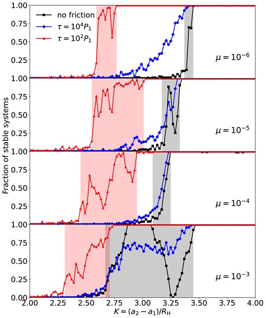
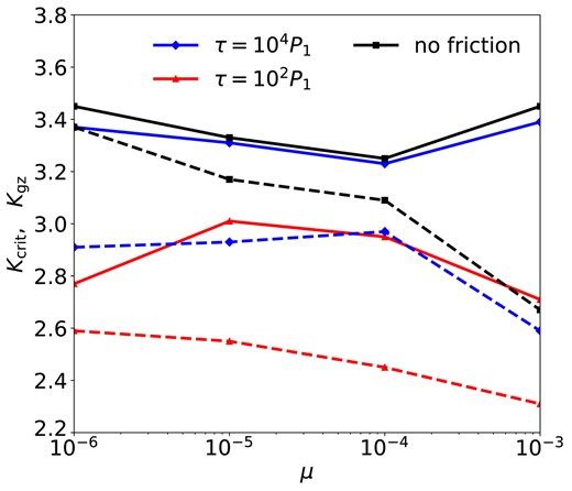
Fig. 1 shows the fraction of stable runs in each suite of simulations as functions of the initial K’s, where the fractions are evaluated by partitioning all runs into 100 bins of width ΔK = 0.02. In all four panels (which present four different mass ratios μ), the systems are mostly (nearly 100 per cent) unstable at small enough K’s and always stable when K is larger than a critical value. Between the stable and unstable regimes, there exist a ‘grey zone’ where the outcomes of the orbital evolution are not guaranteed: some systems become unstable and some remain long-term stable. The exact range of the ‘grey zone’ is not self-evident, so we nominally define ‘grey zone’ to be where the stability fraction is between 10 per cent and 90 per cent. We denote the left and right boundaries of the ‘grey zone’ as Kgz and Kcrit, respectively: systems with K < Kgz have chances of less than 10 per cent to be stable, while systems with K > Kcrit have long-term stable fractions higher than 90 per cent. Fig. 2 shows the values of Kgz (dashed black curve) and Kcrit (solid black curve) for different μ’s.
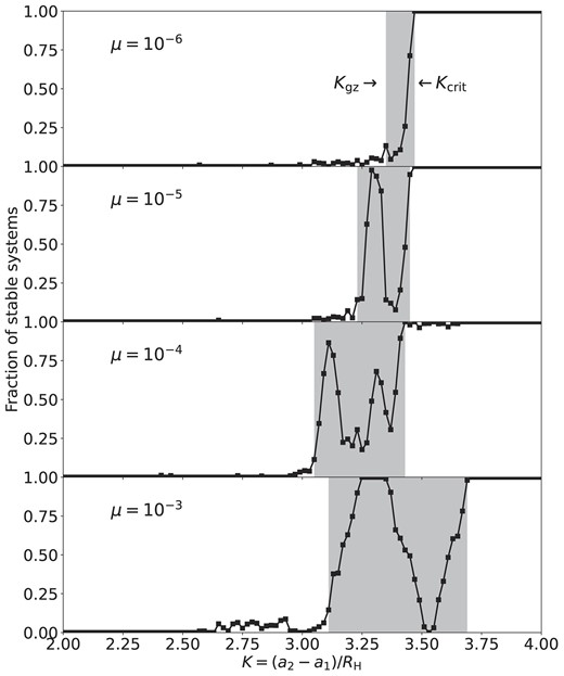
Fraction of stable runs for systems with different μ and initial K in the ‘planet + test mass’ simulations with no frictional force, where the fractions are evaluated by partitioning all runs into 100 bins of width ΔK = 0.02. The ‘grey-zone’ region (the shaded area between Kgz and Kcrit) starts at the minimum K with stable fraction |$\gt 10~{{\ \rm per\ cent}}$| and ends where the stable fraction reaches 90 per cent.
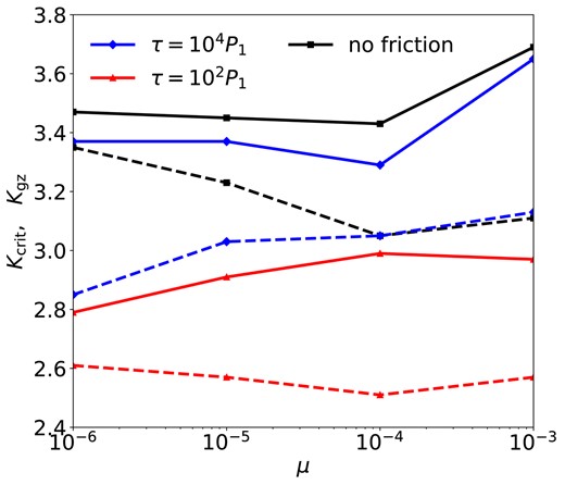
Simulation results of Kcrit (solid) and Kgz (dashed) in ‘planet + test mass’ systems with different μ and frictional forces. Systems with initial K > Kcrit are long-term stable, and those with initial K < Kgz are unstable. Those with initial K between Kcrit and Kgz are in the ‘grey zone’ (defined in Section 2.2.1 and shown in Fig. 1). Here and hereinafter, we use black (squares), blue (diamonds), and red (triangles) only to show the results from simulation with no friction, τ = 104P1 and τ = 102P1, respectively, unless specified otherwise.
In the ‘grey zones’ for μ = 10−5, 10−4, and 10−3, the stability fractions show complex fluctuations and several prominent islands of stability (e.g. near K = 3.3 in the μ = 10−5 runs and K = 3.1 in the μ = 10−4 runs). These islands may be related to mean-motion resonances. We provide an analysis on the origin of these islands using an iterative map in Appendix A.
We summarize in Table 1 the meanings of different kinds of K’s, including Kcrit, Kgz, and those that will be defined later in this paper.
Summary of different K’s defined in this paper. For each symbol in the leftmost column, the remaining columns give a brief description of the symbol, how we evaluate it, and the section where it is first defined.
Summary of different K’s defined in this paper. For each symbol in the leftmost column, the remaining columns give a brief description of the symbol, how we evaluate it, and the section where it is first defined.
2.2.2 Instability time-scale
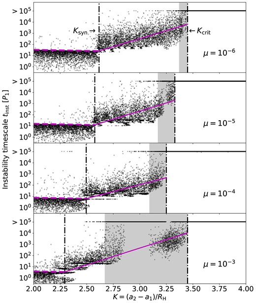
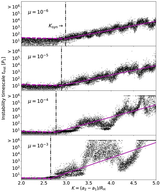
To better understand the growth of instability in our simulations, we characterize the ‘degree of instability’ of each system by tinst, the time for the instability to develop from two initially circular orbits. Fig. 3 shows the tinst from our simulations, with systems that remain stable at 105P1 also included as the tinst > 105P1 dots.
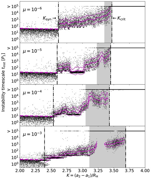
Instability time-scale tinst (black dots) for the simulations shown in Fig. 1. The vertical dashed lines indicate Ksyn and Kcrit, and the ‘grey zones’ (between Kgz and Kcrit) are shaded. At K ≤ Ksyn, the dashed magenta lines mark the synodic period between the test mass and the planet. The solid magenta curves indicate the average time-scales and their ±σ limits (calculated based on the log10tinst’s in each K bin) in the regions between Ksyn and Kcrit.
When K is small, tinst tends to be less than the synodic period Tsyn of the test mass and the planet, where
where P1 and P2 are the initial orbital periods of m1 and m2. This means that the planet-to-test-particle gravity is strong enough to immediately destabilize when the systems when the two orbits are in conjunction. When K exceeds a limiting value, tinst abruptly becomes more likely to be greater than Tsyn. We denote this limiting value as Ksyn and find Ksyn = 2.62, 2.60, 2.54, and 2.39 for μ = 10−6, 10−5, 10−4, and 10−3, respectively (see Fig. 3).
Between Ksyn and Kcrit, the instability takes tinst ≫ Tsyn to develop. The instability time-scale tinst is roughly an exponential function of K. However, there are some zones where the tinst deviates from the exponential trend (e.g. around K ≈ 2.9 and 3.3 for μ = 10−5 and K ≈ 3.3 for μ = 10−3). The random selections of the initial test-mass longitude also introduce a spread for the tinst’s around each K. We calculate the mean time-scale |$\langle$|log10tinst|$\rangle$| and the standard deviation σstd(log10tinst) for each K bin. The data points with tinst > 105P1 are excluded from the calculation. The magenta curves in Fig. 3 shows |$\langle$|log10tinst|$\rangle$| and |$\langle$|log10tinst|$\rangle$| ±σstd(log10tinst) as functions of K.
2.3 Systems with frictional force
2.3.1 Critical spacing for stability
Planets embedded in gaseous discs are subject to ‘frictional’ forces that may induce eccentricity damping and orbital migrations. For example, a low-mass (non-gap opening) planet (of mass m and semimajor axis a) experiences eccentricity damping on the time-scale (e.g. Tanaka & Ward 2004)
where Σ is the disc surface density and h is the aspect ratio, and we have adopted some representative numbers for protoplanetary discs.
To assess the effect of the disc eccentricity damping on the dynamical instability, we re-run the simulations in Section 2.2 with an extra force (see Papaloizou & Larwood 2000 except that their expression carries a factor of 2),
applied to the test mass, where |$\boldsymbol{v}$| is the test mass velocity and |$\hat{r}$| is the radial unit vector. For e ≪ 1, this force leads to eccentricity damping |$\dot{e} \simeq -e/2\tau$|. We have also experimented with a different frictional force model with
where |$\boldsymbol{v}_{\rm K}=\sqrt{\mathrm{ GM}/|\boldsymbol{r}|}\hat{\phi }$| is the Keplerian velocity at the location of the test mass. This force also gives |$\dot{e} \simeq -e/2\tau$|. We found that the effect of equation (7) on the stability of the ‘planet + test particle’ system is similar to that of equation (6). Note that |$\dot{e} \propto -e$| is not the only possible planetary eccentricity evolution in protoplanetary discs. We use |$\dot{e} \simeq -e/2\tau$| because hydrodynamics simulations exploring the eccentricity damping due to planet–disc interactions often express their results in term of τ (e.g. Cresswell et al. 2007; Li et al. 2019; Pichierri, Bitsch & Lega 2022).
Compared to the eccentricity damping, planetary migration takes place a much longer time-scale (e.g. see Papaloizou & Larwood 2000 and Tanaka; Takeuchi & Ward 2002 for type-I migration and Lin & Papaloizou 1986 and Kanagawa, Tanaka & Szuszkiewicz 2018 for type-II). Hence, in this study, we consider the impact of migration to be small and do not include any explicit radial migration in our simulations.2
In the rest of this paper, frictional forces in our N-body simulations are always implemented using equation (6) with τ being a constant in each run.
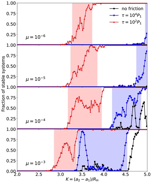
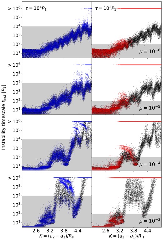
Fig. 4 shows the fraction of stable runs when the frictional force is applied. The blue curves show the results from the weak-friction cases with τ = 104P1. The effects of friction on stability mainly manifest in the ‘grey zones’. First, in low-mass systems (μ ≤ 10−5), the τ = 104P1 friction causes the ‘grey zones’ to span much wider ranges compared to the no-friction counterparts (see also Fig. 2). The ‘grey zone’ in the μ = 10−6 runs has a new left edge extending to Kgz = 2.85. Similarly, Kgz becomes 3.03 in the μ = 10−5 runs. Second, in high-mass systems (μ ≥ 10−5), the friction force tends to relieve the stability islands and straighten the stability fraction curve. As a result, the fraction of stable systems can actually decrease around these stable islands. Overall, as the stable fraction changes from 0 to 1 with increasing K, the τ = 104P1 friction tends to smooth out this process by enlarging the ‘grey zone’ and suppressing the fluctuations in the stability fraction curve.
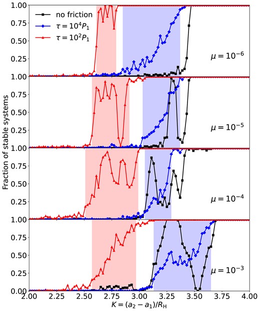
Same as Fig. 1, except also showing the results when the frictional force (equation 6) is applied on the test particle. The red lines show the cases with τ = 102P1 and the blue lines with τ = 104P1. The black lines are from the no-friction results (same as in Fig. 1). The red and blue shades are the ‘grey zones’ for the τ = 102P1 and τ = 104P1, respectively.
The red curves in Fig. 4 show the results from the strong-friction case with τ = 102P1. Compared with the no-friction and weak-friction cases, the strong-friction runs achieve long-term stability at smaller K values. The systems in the original ‘grey zones’ are almost fully stabilized by the frictional force, while new ‘grey zones’ appear at around K = 2.75 (see also Fig. 2). Strong fluctuations again appear in the stability fraction curves.
In summary, the onset of stability remains complicated when friction is considered. We compress the complexities into the so-called grey zones, where the fraction of the stable systems may fluctuate between 10 per cent and 90 per cent. Frictional forces can change the sizes and locations of the ‘grey zones’ and affect how stability fluctuates. We numerically determine the left and right boundaries of each ‘grey zone’ and show the results in Fig. 2. The right boundary, Kcrit, represents the critical spacing for stability; the left boundary, Kgz, can be considered as the onset of the brief precursory fickleness.
2.3.2 Instability time-scale
Fig. 5 compares the tinst results from the with-friction runs (coloured dots) to those from the no-friction runs (black dots). We shade the area with tinst ∈ [0, τ]. Inside the shaded area, the instability growth is faster than the eccentricity damping (tinst < τ), so the with-friction and no-friction runs show a similar distribution of tinst. Outside of the shaded area, the instability is weaker (tinst > τ), so the systems can be stabilized by the frictional force; thus, the black dots are not covered by the coloured dots as the coloured dots are pushed upward to the simulation time limit at tinst > 105P1. The outlying coloured dots at around K ≈ 3.25 with tinst ∈ [τ, 105P1] in the bottom left panel of Fig. 5 are systems that are previously inside a stability island but now destabilized by the damping force.
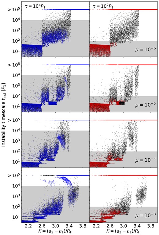
Instability time-scale tinst for ‘planet + test mass’ systems with frictional force applied. The blue dots show the results of the τ = 104P1 cases, and the red dots show the results of the τ = 102P1 cases. The black dots are the no-friction results (same as in Fig. 3). The regions with tinst ∈ (0, τ) are shaded.
Several features of the ‘grey zones’ (see Fig. 4) can be related to the distribution of tinst’s. First, the sizes of the ‘grey zones’ are mainly determined by the vertical spreads of tinst: a constant damping time-scale τ can cut across the distribution of tinst’s over a wide range of K values; this range becomes the ‘grey zones’ as only some of the systems in this range can be stabilized by the friction. Second, the fluctuation of the stable fraction is caused by the irregular variation of tinst. Frictional forces with different τ values reveal different regions of this irregular variation, thus producing anomalies in the stable fraction curves.
3 INSTABILITY IN TWO-PLANET SYSTEMS
3.1 Setup of the simulations
In this section, we study systems with two (non-zero mass) planets using N-body simulations. Our simulated systems consist of a central star with mass M, an inner planet with mass m1 = 2 μM, and an outer planet with mass m2 = μM. Same as in the previous section, the initial orbital separation between the planets is set as
where RH is calculated by equation (2). We consider μ = 10−6, 10−5, 10−4, and 10−3. All planets are co-planar and initially on circular orbits, and their initial longitudes are sampled randomly. For the simulations with friction, we apply equation (6) to all planets to model the frictional damping.
3.2 Critical spacing for stability
For each μ-value, we perform a suite of 10 000 simulations with the initial K’s sampled randomly from a uniform distribution in the range of K ∈ [2, 4]. We run the simulations up to 105P1 and repeat all suites three times for ‘no-friction’, τ = 102P1, and τ = 104P1.
Fig. 6 shows the fraction of stable runs in two-planet simulations. The black curves show the results from the no-friction cases. Unlike the test-mass runs (see Fig. 1), the ‘grey zones’ for two-planet systems do not contain as many stability islands, except at K = 3.23 for μ = 10−5 and from K = 2.87 to 3.07 for μ = 10−3.
Similar to Fig. 4, except showing the fraction of stable runs for systems with two finite-mass planets (m1 = 2m2 = 2μM) after 105P1. The black lines are from the ‘no-friction’ runs. The red lines show the cases with τ = 102P1 and the blue lines show the cases with τ = 104P1. The black and the red shades represent the ‘grey zones’ for the no-friction and the τ = 102P1 runs, respectively. (The ‘grey zone’ for τ = 104P1 is not shown to avoid overlaps between the shades.)
The blue curves show the results from the weak-friction (τ = 104P1) cases. Same as in the test-mass runs, ‘grey zones’ tend to expand toward smaller K, especially when μ = 10−6 and 10−5; the stability islands that exist in the no-friction results (black curves) are leveled out.
The red curves show the results from the strong-friction (τ = 102P1) cases, where the ‘grey zones’ shift to around K = 2.75 and the stable fractions become fluctuating again (as opposed to the weak-friction results).
Fig. 7 summarizes the values of Kgz and Kcrit (the left and right boundaries of the ‘grey zone’) in each case.
Similar to Fig. 2, except showing the values of Kcrit (solid) and Kgz (dashed) for systems with two finite-mass planets (m1 = 2m2 = 2μM).
3.3 Instability time-scale
Fig. 8 shows the instability growth time, tinst, from the no-friction simulations (with the systems that remain stable in 105P1 being added as the tinst > 105P1 dots). Similar to the test-mass cases (see Fig. 3), when K is small (≤Ksyn given in the caption of Fig. 8), tinst is almost always less than the synodic period (equation 4) of the two planets: the mutual gravity between the planets is strong enough to trigger immediate instability at their first orbital conjunction.
Similar to Fig. 3, except showing the instability time-scale tinst (black dots) for systems with two finite-mass planets (m1 = 2m2 = 2μM). No friction force is applied. The vertical dash–dotted lines indicate Ksyn and Kcrit, and the ‘grey-zone’ regions are shaded. At K ≤ Ksyn, the dashed magenta lines mark the synodic period between the two planets. The solid magenta lines show the fitting formulae using equation (9) in the region from Ksyn to Kcrit. From the top to the bottom panel, we find that (Ksyn, Tsyn, 0, b) are (2.62, 25.98P1, 2.88), (2.58, 12.52P1, 2.92), (2.49, 6.26P1, 2.48) and (2.29, 3.42P1, 3.02), respectively.
Between Ksyn and Kcrit, the instability growth time tinst can vary by several orders of magnitude for the same μ and K. The ‘typical’ instability time is roughly an exponential function of K. We fit the data points in the transition region with
using the least-squares method, where Tsyn,0 is the synodic period when K = Ksyn. The data points with tinst > 105P1 are excluded from the fitting. The fitting results are shown as the solid magenta lines in Fig. 8, and the values of the parameters are given in the caption.
Fig. 9 compares tinst’s from the with-friction runs (coloured dots) to the results from the no-friction runs (black dots). Similar to Fig. 5, instability can only happen inside the shaded area with tinst ∈ [0, τ] (except for when μ = 10−3 and τ = 104P1). Outside of the shaded area, tinst > τ and instability is suppressed. The ‘grey zones’ are the ranges of K where only a portion of runs are stabilized (i.e. where only a part of the black dots are covered by the colour dots).

Similar to Fig. 5, but showing the instability time tinst for two-planet systems (m1 = 2m2 = 2μM) with frictional force applied. The red dots show the results from the τ = 102P1 cases and the blue dots show those from the τ = 104P1 cases. The black dots are from the no-friction runs (same as in Fig. 8).
Knowing the trend of tinst allows us to estimate the critical orbital spacing for stability. For each μ and τ, we calculate
where the first term in the curly brackets is obtained by setting tinst = τ in equation (9), and the latter term Kcrit, ∞ is equal to the value of Kcrit from the no-friction simulations. This Kcrit,∞ term is to ensure that |$K^{\rm (est)}_{{\rm crit},\tau }$| for a finite τ is not greater than the critical spacing when τ = +∞. We use |$K^{\rm (est)}_{{\rm crit},\tau }$| as an estimation of Kcrit for different τ: with initial |$K\gt K^{\rm (est)}_{{\rm crit},\tau }$|, a system is expected to have tinst > τ, so the system is expected to be stable, and vice versa. Fig. 10 compares |$K^{\rm (est)}_{{\rm crit},\tau }$| from equation (10) to Kcrit from the simulations. The red lines show that, when τ = 102P1, |$K^{\rm (est)}_{{\rm crit}, \tau }$| can accurately estimate Kcrit with an error always less than 0.2. For τ = 104P1, |$K^{\rm (est)}_{{\rm crit}, \tau }$| (dotted blue) differs from the numerical Kcrit (solid blue) by less than 0.1 for all μ. We note that, when τ = 104P1, the first term on the right-hand side of equation (10) is always greater than Kcrit,∞ (which is given by the solid black line in Fig. 7); hence, |$K^{\rm (est)}_{{\rm crit}, \tau }$| is equal to Kcrit,∞ for all μ. Conversely, if |$K^{\rm (est)}_{{\rm crit}, \tau }$| were defined to be always equal to the first term on the right-hand side of equation (10) rather than the smaller term of the two, it would become less accurate.
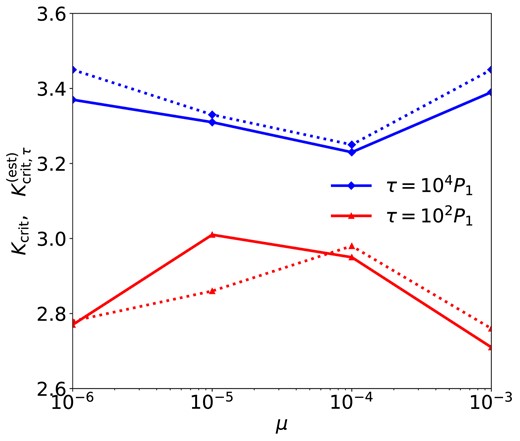
Values of Kcrit (solid) and |$K^{\rm (est)}_{{\rm crit},\tau }$| (dotted) in two-planet systems (m1 = 2m2 = 2μM) with different μ and frictional forces. Kcrit is the critical orbital spacing for stability derived by simulations, while |$K^{\rm (est)}_{{\rm crit},\tau }$| is an estimation of Kcrit calculated by equation (10). Note that for τ = 104P1, |$K^{\rm (est)}_{{\rm crit},\tau }$| equals Kcrit,∞, which is equal to the value of Kcrit in the no-friction simulations.
4 INSTABILITY IN THREE-PLANET SYSTEMS
4.1 Setup of the simulations
It has been well recognized that stability in two-planet systems and that in systems with more than two planets are substantially different: the Hill stability criterion only applies to two-planet systems; systems with three or more planets can become unstable even when the initial planetary separations are large, although the instability growth time increases rapidly with the separation (see Pu & Wu 2015 and refs therein).
Our simulations in this section are for systems consisting of a central star with mass M and three planets. The planets have masses m1 = 2μM, m2 = μM, and m3 = 0.5μM in Sections 4.2 and 4.3, and m1 = m2 = m3 = μM in Section 4.4. The initial orbital separation between two neighbouring planets is set as
where K is the same dimensionless orbital separation for all neighbouring pairs and
is the mutual Hill radius of mj and mj + 1. Same as in the previous sections, we consider μ = 10−6, 10−5, 10−4, and 10−3. All planets are co-planar and initially on circular orbits. Their initial longitudes are sampled randomly. For some experiments, we apply equation (6) to all planets to model the frictional damping.
4.2 Critical spacing for stability
For each μ-value (with planet masses m1 = 2m2 = 4m3 = 2μM), we perform a suite of 10 000 simulations with randomly sampled initial K’s. Because the Hill criterion of stability does not apply in systems with more than two planets, we investigate a wider range of the initial K ∈ [2, 5], and run the simulations up to 106P1. We repeat each suite three times for ‘no-friction’, τ = 102P1, and τ = 104P1.
Fig. 11 summarizes the fraction of systems that remain stable at the end of our simulations. In the no-friction runs (black curves), most of the runs become unstable within 106P1; we expect the stable fraction to converge to zero for all considered K values if we evolve the systems for more orbits.
Same as Fig. 4, except showing the stable fraction for three-unequal-mass planet systems (m1 = 2m2 = 4m3 = 2μM) after 106P1. We expect the stable fraction (black curves with square markers) to converge to zero for all considered K values if we evolve the systems for much more orbits.
When the frictional force with τ = 104P1 is applied (blue curves), the survival rate increases at large K. Notably, around 80 per cent of the systems with μ = 10−6 and 10−5 are stable at K = 5.0; hence, they should have Kcrit ≳ 5. Systems with μ = 10−4 have a nearly 100 per cent chance to be stable at K = 5.0 and more than 50 per cent chance to survive at K ≳ 4.5. In the μ = 10−3 case, all simulations with K ≳ 4.7 are stable.
When τ = 102P1 (red curves), almost all systems are stable at K > 4. A large fraction of the systems become stable at around K ≈ 3.4.
The left panel of Fig. 12 summarizes the values of Kgz and Kcrit (the left and right boundaries of the ‘grey zone’) in the simulations with frictional forces. There are no ‘grey zones’ for the no-friction systems.
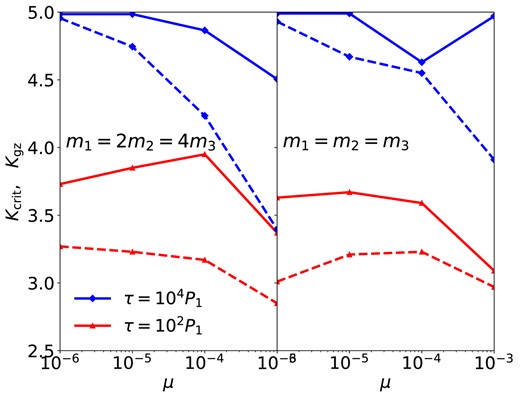
Similar to Fig. 2, except showing the values of Kcrit (solid) and Kgz (dashed) for systems with three planets. Systems with m1 = 2m2 = 4m3 = 2μM are shown on the left, and systems with m1 = m2 = m3 = μM are on the right. Without friction, no systems are expected to be long-term stable (no Kcrit, Kgz or ‘grey zones’).
4.3 Instability time-scale
Fig. 13 shows the instability growth time tinst in the no-friction systems.3 All runs have tinst < 106P1, except at (1) K ≥ 4.6 for μ = 10−3, where tinst is longer than the time limit of the simulations due to the large initial planet spacings, and (2) K = 3.8 for μ = 10−3 and K = 4.7 and 4.9 for μ = 10−4, where tinst are larger than at their neighbouring K’s (possibly due to mean-motion resonances and chaos, see e.g. Lissauer & Gavino 2021). Systems with lower μ tend to have smaller fluctuation amplitude for tinst. We find the value of Ksyn for each μ using the synodic period of the two inner planets and fit the data points with K > Ksyn and tinst < 106P1 using equation (9). The results are listed in the caption of Fig. 13.
Same as Fig. 8, but for systems with three-unequal-mass planets (m1 = 2m2 = 4m3 = 2μM). The vertical–dotted lines indicate Ksyn, while Kcrit does not exist. From the top to the bottom panel, we find that (Ksyn, Tsyn,0, b) are (2.98, 22.84P1, 1.26), (2.89, 11.20P1, 1.37), (2.77, 5.69P1, 1.78), and (2.65, 3.03P1, 2.23), respectively.
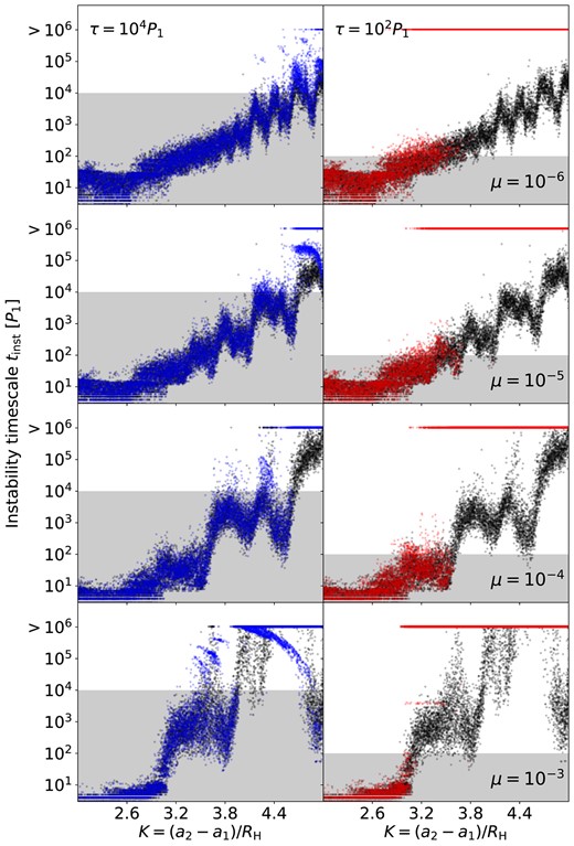
Fig. 14 displays tinst when the frictional force is applied. Unlike in Figs 5 and 9, there exists systems with tinst > τ in all panels of Fig. 14. The stability of a three-planet system can be assured only if tinst ≳ 10−100τ. Systems with tinst ≈ τ are expected to be in the ‘grey zones’.
Same as Fig. 9, but for systems consisting of three planets with m1 = 2m2 = 4m3 = 2μM.
We fit tinst with equation (9), show the fitting results in Fig. 13, and calculate
for each μ and τ; this expression is the same as equation (10) but with Kcrit,∞ being infinite; then we compare them with the empirical Kcrit in the left panel of Fig. 15. At τ = 104P1 and μ ≤ 10−5, Kcrit is bounded at five by the upper limit of our parameter space, while |$K^{\rm (est)}_{{\rm crit},\tau }$| is slightly greater than five as calculated by the fitting formula. For other τ and μ, |$K^{\rm (est)}_{{\rm crit},\tau }$| is less than Kcrit (because tinst = τ is in the grey zone, see Fig. 14), but the difference is always smaller than 0.5. As an application of this result, one can calculate |$K^{\rm (est)}_{{\rm crit},\tau }$| for different values of τ to get a decent estimation of the critical orbital spacing for the long-term stability of three-planet systems.
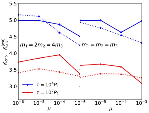
Similar to Fig. 10, except showing the values of Kcrit (solid) and |$K^{\rm (est)}_{{\rm crit},\tau }$| (dotted) for three-planet systems. Systems with m1 = 2m2 = 4m3 = 2μM are shown on the left; systems with m1 = m2 = m3 = μM are on the right.
4.4 Dependence on the planetary mass distribution
In this paper, we focus on the stability of systems with different μ, which is the planet-to-star mass ratio. In general, stability can also be affected by the mass ratios between the planets. To probe the effect of the planetary mass distribution, we repeat our three-planet simulations but with m1 = m2 = m3 = μM.
The resulting Kcrit and Kgz from the equal-mass simulations are shown in the right panel of Fig. 12. We find that, when μ is small, equal-mass systems and those with outward-decreasing mass distributions have similar Kcrit’s and ‘grey zones’. However, when μ = 10−4, equal-mass systems have a much narrower ‘grey zone’ for both values of τ. When μ = 10−3 and τ = 104P1, equal-mass systems have Kcrit = 4.97 and Kgz = 3.91, which are both larger than the outward-decreasing-mass values; when τ = 102P1, the ‘grey zone’ is confined bewteen Kcrit = 3.09 and Kgz = 2.97.
Fig. 16 shows tinst for equal-mass systems. Same as in the outward-decreasing cases, tinst is an exponential function of K but with local spreads and fluctuations. The amplitudes of these fluctuations are large when μ is big. Frictional stabilization operates similarly in equal-mass cases to those with unequal masses (Fig. 14): systems are most likely to remain stable when tinst ≳ 10–100τ. We fit tinst with equation (9) for each μ and τ and show the fitting results in Fig. 16’s caption. We calculate |$K^{\rm (est)}_{{\rm crit},\tau }$| (with equation 13 and the fitting results4 in Fig. 16) and show the results in the right panel of Fig. 15.
Same as Fig. 14, but for systems with three equal-mass planets with m1 = m2 = m3 = μM. From the top to the bottom row, we find that the no-friction results (black dots) can be fitted with (Ksyn, Tsyn,0, b) as (2.80, 27.72P1, 1.12), (2.77, 13.28P1, 1.45), (2.68, 6.64P1, 1.71), and (2.50, 3.57P1, 1.90), respectively.
In summary, the results for the two types of mass configuration are similar when μ = 10−6 and 10−5 but different when μ = 10−4 and μ = 10−3. This is because large-μ cases tend to have more significant tinst fluctuations.
5 CONCLUSION
5.1 Summary of key results
In this paper, we have studied the dynamical instability of closely packed multiplanet systems in the presence of frictional forces that arise from planet–disc interactions. The systems have initially coplanar and circular orbits with the orbital separation characterized by the dimensionless ratio K = (aj + 1 − aj)/RH (where aj is the semimajor axis of the j-th planet, and RH is the mutual Hill radius). Instability occurs due to planetary orbital crossing (see equation 3) as the system evolves. The goal of this paper is to evaluate how frictional forces (of various strengths) affect the growth of instability as a function of K and the planet-to-star mass ratio μ. Note that although we use the terms ‘planet’ and ‘star’ throughout this paper, our results are also relevant for understanding the evolution of stellar-mass black holes embedded in AGN discs around supermassive black holes.
We consider both ‘2 planets’ and ‘3 planets’ systems using numerical N-body integrations. (For analytical understanding, see Appendix A, where we carry out theoretical analysis of the restricted three-body problem consisting of star, planet, and test particle). For each planetary architecture, we adopt a range of planet-to-star mass ratios (μ), initial dimensionless orbital separations (K), and frictional damping time-scales (τ), and determine the fraction of stable systems and instability growth time tinst (i.e. the time to reach the first orbital crossing from initially circular orbits).
The main result of this paper concerns the stability as a function of K and τ. In general, we find that the stable (large K) and the unstable (small K) regimes are separated by a ‘grey zone’. Inside the ‘grey zone’, there is no guarantee whether dynamical instability will occur or not: the probability for a system in the ‘grey zone’ to be long-term stable is between 10 per cent and 90 per cent5 and does not always increase monotonically with K. Specifically:
For ‘planet + test mass’ and ‘2 planets’ simulations, the stability fractions and the ‘grey zones’ are shown in Figs 1, 4, and 6. We summarize and compare the ranges of ‘grey zones’ in Figs 2 and 7. The right boundary, Kcrit, can be considered as the critical spacing for stability: while frictionless systems have |$K_{\rm crit} \simeq 2\sqrt{3}$|, frictional forces tend to stabilize more systems by pushing Kcrit towards smaller values.
For ‘3 planets’ simulations, long-term stabilities (and ‘grey zones’) appear when frictional forces are applied (Fig. 11). We show the left and right boundaries of ‘grey zones’ in Fig. 12: frictional damping with τ = 104 is needed for most systems to be stable at K = 5 and τ = 102 is needed at K = 4.
To better understand our results, we analyse the time-scale to instability tinst:
The instability time-scales tinst for different planetary architectures are shown in Figs 3, 8, and 13. For systems with the same μ and initial K, tinst can vary by up to 3 orders of magnitude due to its dependence on the initial orbital phases of the planets.
When K ≤ Ksyn, most simulations exhibit tinst < Tsyn (the synodic period), i.e. the instability occurs at the first orbital conjunction. When K > Ksyn, the average tinst is roughly an exponential function of K (equation 9), although it also shows many fluctuations.
To be stabilized (i.e. to bypass the ‘grey zone’), a two-planet system needs to have tinst ≳ τ (see Figs 5 and 9) and a three-planet system needs to have tinst ≳ 10τ –100τ (see Fig. 14).
Given τ, we use the fitting formula for tinst-versus-K (equation 9) to find a special |$K^{\rm (est)}_{{\rm crit},\tau }$| (equations 10 and 13) such that tinst = τ when |$K=K^{\rm (est)}_{{\rm crit},\tau }$|. Figs 10 and 15 show the values of |$K^{\rm (est)}_{{\rm crit},\tau }$|, and suggest that |$K^{\rm (est)}_{{\rm crit},\tau }$| provides a decent estimate to the numerical Kcrit (with errors less than 0.5).
In addition, the stable fractions show complex fluctuations with several prominent islands of stability inside the ‘grey zones’. We find that weak frictional forces may flatten those stability islands, causing the planet survival fraction to decrease in those islands and making the stable-fraction-versus-K curve smoother inside the ‘grey zones’.
5.2 Discussion
Our results are useful for understanding the evolution of multiplanet systems born in protoplanetary discs, and the evolution of multiple stellar-mass black holes BHs in AGN discs (see Section 1). Multiple planets can be brought into closely packed orbits due to differential migration or migration traps in the disc. The frictional forces from the disc acting on the planets can help maintain the stability of the system even for small planetary spacings – ‘how small’ depends on the frictional damping time-scale, which in term depends on the disc density.
To use our results: (i) one can refer to Figs 2, 7, and 12, where we have numerically determined the critical spacing for stability, Kcrit, for systems with different orbiter masses and damping time-scales. For damping time-scales that have not been simulated in this paper, one can use |$K^{\rm (est)}_{{\rm crit},\tau }$| (defined by equations 10 and 13) to estimate the critical spacing needed to ensure stability with an accuracy of |$|K^{\rm (est)}_{{\rm crit},\tau }-K_{\rm crit}|\lt 0.5$|. (ii) Our result for Kgz provides upper limits of the regime where stability is almost impossible. (iii) For systems inside the ‘grey zone’ (K ∈ [Kgz, Kcrit]), numerical simulations are needed to determine their long-term stability.
In this paper, we have focused on the onset of dynamical instability, signalled by close encounters between two planets (see equation 3). Once the instability is initiated, the system will experience chaotic orbital evolution. In the absence of gas friction, close encounters keep recurring until one planet is ejected, two planets collide with each other, or one planet crashes into the star. The branching ratio of each outcome depends on the planetary mass, radius, and orbital velocity around the host star (see Li et al. 2021a and references therein). In the case of stellar-mass BHs around a supermassive BH, the large mass ratio implies that ejection is highly unlikely or impossible; and the chaotic orbital evolution is terminated when two BHs undergo an extremely close encounter and form a bound, merging binary due to gravitational radiation (see Li, Lai & Rodet 2022a and references therein).
When dynamical instability develops in the presence of gas discs, there exists another possible outcome in which the system regains its stability after the chaotic evolution: the combined effects of close encounters and frictional forces may push the planets (or BHs) into well-separated orbits to ensure dynamical stability with friction (Li, Lai & Rodet 2022a). In particular, we expect that frictional forces may prevent some planetary ejections and star crashings because they typically require a large number of closer encounters than planet–planet collisions.
ACKNOWLEDGEMENTS
We thank the anonymous reviewer for very helpful comments that improve the clarity of this paper. We also thank Yuji Matsumoto and Sean Raymond for their helpful suggestions. This work was supported by National Science Foundation grant AST-2107796 and the National Aeronautics and Space Administration grant 80NSSC19K0444. JL was supported by the Center for Space and Earth Science at Los Alamos National Laboratory (approved for public release as LA-UR-22-23672). This research used resources provided by the Los Alamos National Laboratory Institutional Computing Program, which was supported by the U.S. Department of Energy National Nuclear Security Administration under Contract No. 89233218CNA000001.
DATA AVAILABILITY
The data underlying this article will be shared on reasonable request to the corresponding author.
Footnotes
In the remainder of this paper, we shall use the terms ‘planet’ and ‘star’, although they could be ‘BH’ and ‘supermassive BH’.
We note that equation (6) can already cause a radial migration rate |$\dot{a}/a\simeq e^2/\tau$| implicitly because it represents a torque-free forcing (e.g. Ataiee & Kley 2021). In principle, this effect might also impact the stability of a system by changing the planetary orbital spacing in time. However, we find that the test particle has a final eccentricity e ≲ 0.1 in most of our stable runs in Section 2.2 (including those inside the stable islands), and we think the effect of |$\dot{a}$| due to equation (6) is negligible.
Petit et al. (2020) provide an analytical expression (see their equation 81) that can predict tinst in three-planet systems. Applying their formula to the systems in Fig. 13, we find that the predicted tinst is less than 104P1 when μ ≤ 10−4 and K ≤ 5, less than 106P1 when μ = 10−3 and K ≲ 4.8, and diverge to infinite when μ = 10−3 and K > 4.8. These predictions are roughly consistent with most of our simulation results. However, because the formula in Petit et al. (2020) predicts a smooth and monotonic tinst-versus-K relation, it does not describe the large tinst fluctuations shown in Fig. 13.
We note that Chambers, Wetherill & Boss (1996) have also studied the μ = 10−5 case in the no-friction scenario (same as black dots in the second row of our Fig. 16); their results can be fit by log10(tinst) ≈ 1.69K − 3.97. Our fitting result, (Ksyn, Tsyn,0, b) = (2.77, 13.28P1, 1.45) as shown in the caption of Fig. 16, is equivalent to log10(tinst) = 1.45K − 2.38. This discrepancy may be due to differences in the sample size, the range of K (which is up to five in this paper and six in Chambers, Wetherill & Boss 1996), and the expression of log10(tinst). Nevertheless, we find that our fitting formula also fits the data points in Chambers, Wetherill & Boss (1996) very well when K ≤ 5.
We use 10 per cent and 90 per cent as the nominal boundaries of the ‘grey zone’ because, in most cases throughout this paper, they provide a good covering of the parameter region where the stability friction goes from small to large. See also Section 2.2.1.
References
APPENDIX A: A LINEAR MAP ANALYSIS OF THE STABILITY OF THE RESTRICTED THREE-BODY PROBLEM
A1 Formalism of the linear map
In this section, we present an analytical map that can qualitatively reproduce the simulation results of Section 2. Our approach is modified and generalized from the previous work by Duncan, Quinn & Tremaine (1989; hereafter DQT89).
We map the evolution of the outer test particle’s orbit to a succession of conjunctions with the inner planet. The leading-order change of the orbital elements of the test mass during a conjunction can be derived using the shearing box framework (Henon & Petit 1986). We define
where K0 and K1 are the modified Bessel functions of the second kind, and the subscript p denotes the massive planet. We define zn to be the complex eccentricity just after the nth conjunction, and zn− the complex eccentricity just before the nth conjunction (see Fig. A1). We use the same notations for the relative semimajor axis ε and the longitude λ of the test mass at the conjunction. During the nth conjunction, the complex eccentricity is changed by the amount (see DQT89)
and the following quantity (Jacobi integral) is conserved
In DQT89, ε is fixed to εn− in equation (A4), an approximation that becomes incorrect close to the instability boundary, where ε can vary significantly. In this work, we use a leap-frog-like approach to evaluate εn,mid, the average of the pre-conjunction and the estimated post-conjunction ε-values:
The actual post-conjunction orbital elements are
In the no-damping case, the orbital elements are conserved between the conjunctions, i.e.
In the damping case, with the frictional force described as in equation (5) (corresponding to an exponential eccentricity damping with time-scale τ), we have at first order:
where Tn is the synodic period after the nth conjunction. It can be derived from the orbital periods of the planet Pp and test particle P:
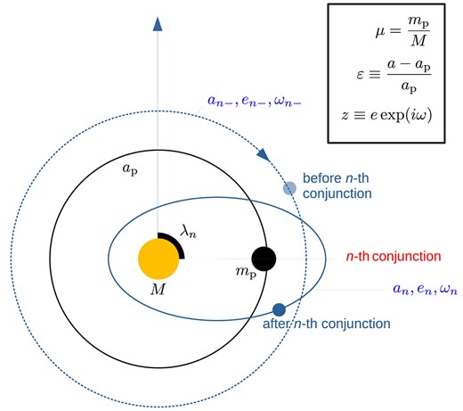
Setup of the linear map and the definition of the key parameters and variables.
Orbital crossings occur when e > ε and equation (3) is met when e ≳ ε − RH/ap. However, both criteria lie outside the validity range of the map (e ≪ ε, see Duncan, Quinn & Tremaine 1989). In the following, we adopt the stability condition
We adopt β = 0.85, which is shown by empirical tests to best reproduce some qualitative features of the N-body results (Section 2).
Starting from e = 0, equating |Δz| (equation A4) to ε gives the Hill radius scaling (ε∝μ1/3). Alternatively, equating the variable part of |λn − λn−| to π gives the resonance overlap criterion scaling (ε∝μ2/7; Wisdom 1980; DQT89; see Appendix B). As we will see below, however, these scalings do not account for the complexity of the instability threshold.
A2 Results
Using the algebraic map described in Section A1, we compute tinst,map, which is the time for a system to reach the limiting eccentricity to break equation (A17). A system is considered stable if it satisfies equation (A17) for 105P1. The initial eccentricity of the test mass is set to be very small but non-zero so that the initial conjunction longitude λ can be well defined. The map calculations in this section are done with the initial eccentricity e = 10−8 and the initial λ ∈ [0, 2π) chosen randomly. We have also experimented with initial e’s that are equal to 10−5, proportional to μ, and proportional the initial ε and found similar results.
Fig. A2 shows the results from the map without friction (i.e. with equations A10–A12). The behaviour of tinst,map with respect to K (for a given μ) resembles that of tinst from the N-body simulations in a few ways:
The average value of tinst,map is roughly an exponential function of K.
At large K, there exist critical values of K for long-term stability.
The map results show several stability islands, such as at K = 3.45 when μ = 10−5 and at K = 2.95 when μ = 10−4.
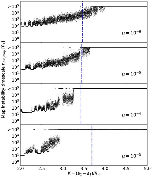
However, we also note that the linear map can be quantitatively inaccurate:
tinst,map tends to show much less fluctuations than tinst.
The map underestimates the values of Kcrit (the critical orbital spacing for stability derived by N-body simulations in Section 2) when μ = 10−4 and 10−3, and overestimates Kcrit when μ = 10−6 and 10−5. Moreover, in the μ = 10−6 case, more systems may become unstable at around K = 4 if they are evolved for more than 105P1.
The locations of the stability islands found by the map are different from those found by N-body simulations.
These discrepancies may be related to the approximations of the map and the quantitative difference between equations (3) and (A17).
Fig. A3 shows tinst,map from the map with the frictional damping included (see equation A13) for two damping time-scales τ = 104P1 and τ = 103P1. We have also experimented with τ = 102P1 and found that most runs are stable. Instability is expected to be stronger than the frictional damping for runs in the shaded area. The result strictly follows our expectation: eccentricity can only grow if tinst,map is inside the shaded area; outside of the shaded area, except for a negligible amount of outliers, no instability is found.

A3 Stability islands
Similar to the N-body simulations (Section 2), the map evaluation also reveals some stability islands. Although the island locations are not exactly the same as in the N-body simulations, the map can offer a qualitative explanation as to why stability islands exist.
We analyse the map by assuming gμ/ε2 ≲ e. Using equations (A7) and (A8) and setting zn− = eexp iω, λn − = λ and |$\varepsilon _{n,\rm {mid}} \simeq \varepsilon _{n-} = \varepsilon$|, we find that, during one conjunction, the orbit of the test mass changes by
where η ≡ gμ/(ε2e) ≲ 1 and ϕ ≡ λ − ω, which is the anomaly of the test mass when it is in conjunction with the planet. Equations (A18) and (A19) imply that the cumulative change of e and ε will be zero if ϕ “librates” (discretely at each conjunction) around ϕ = 0 or π. Note that ϕ = 0 and π mean that the conjunctions happen when the test mass is at its pericentre and apocentre, respectively.
The next conjunction will occur with ϕn = ϕ + Δϕ, where Δϕ = Δλ − Δω. The term Δλ can be calculated using equation (A9) with εn = ε + Δε. In the situation when the orbital periods of the test mass and the planet is in the ratio of (1 + ε)3/2 = (p + 1)/p for an integer p, equation (A9) suggests
With the factor 4πp2e2/ε expected to be a few for the N-body runs inside the stable islands, we get
This allows the test mass to undergo a long-term “libration” of ϕ around ϕ = π, forming islands of long-term stability at some special initial K values.
Fig. A4 shows the results from two of our “planet + test mass” N-body simulations with μ = 10−5 and initial K = 3.3 (blue) and 3.4 (orange). The former is inside a stability island while the latter is outside of the island (see Section 2, Figs 1 and 3).
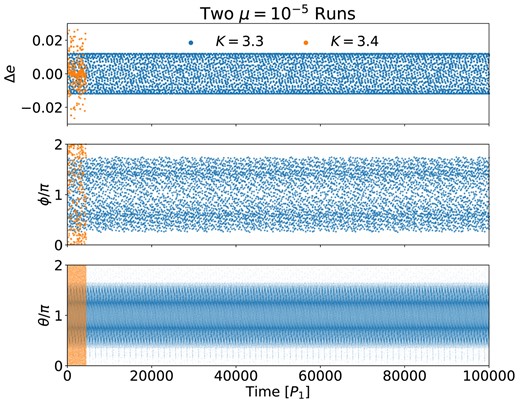
Comparison of two N-body runs in with μ = 10−5. The blue dots are the results of a run with an initial K = 3.3, which represents a system inside the stability island (see the second panel of Fig. 1). The orange dots are the results of a run with an initial K = 3.4, which represents a system outside of the island. The top, middle, and bottom panels show the evolution of Δe (the change of test-mass orbital eccentricity during each conjunction), ϕ (the anomaly of the test mass at each conjunction), and θ = 14λ2 − 13λ1 − ϖ2 (the 14:13 resonance angle at all time), respectively. Quantities Δe and ϕ are only defined when the test mass and the planet are in conjunction. The angles λ1,2 are the mean longitude of the planet and the test mass, and ϖ2 is the longitude of pericentre of the test mass.
The top panel of Fig. A4 displays all Δe’s, which are the changes of test-mass orbital eccentricity during the times when the planet and the test mass are in conjunction. In the stable case (K = 3.3, blue), the Δe’s spread around 0 almost symmetrically at all times, so the cumulative eccentricity change is always small. In the unstable case (K = 3.4, orange), the Δe distribution is random, so the eccentricity of the test mass may grow.
The middle panel of Fig. A4 shows the evolution of ϕ, which is the mean anomaly of the test mass at each conjunction. As we have speculated using the map, ϕ in the stable system undergoes a discrete “liberation” around ϕ = π, while the ϕ in the unstable system takes arbitrary values between 0 and 2π.
The bottom panel of Fig. A4 shows the evolution of one of the 14:13 resonance angles θ = 14λ2 − 13λ1 − ϖ2, where λ1,2 are the mean longitude of the planet and the test mass and ϖ2 is the longitude of pericentre of the test mass. At the time of conjunctions, θ = ϕ. In the stable case with initial K = 3.3, the planet and the test mass have a period ratio of nearly 13:14. Although θ does not liberate continuously as in mean-motion resonances, it still evolves periodically around the θ = π for most of the time. In the unstable case with K = 3.4 initially, θ evolves between [0, 2π] uniformly.
Fig. A5 is the same as Fig. A4, except showing the results from two simulations with μ = 10−4, initial K = 3.1 (blue) and 3.2 (orange), and with θ = 7λ2 − 6λ1 − ϖ2. The results in both Figs A4 and A5 are consistent with the stabilizing mechanism described by the map.

In summary, we have shown that the stability islands can be created by liberations around mean-motion resonances.
APPENDIX B: DERIVATION OF THE MEAN-MOTION RESONANCE OVERLAP SCALING FROM THE LINEAR MAP
This derivation has been proposed by DQT89. Let us consider the first conjunction of the linear map presented in Section A. DQT89 argues that the onset of chaos occurs when the variable part of the conjunction longitude difference |λn − λn−| is similar or greater than π. From equation (A9), we have
where Δε = ϵ1 − ϵ1−. DQT89’s condition thus writes:
We assume that the orbits are initially circular, so that Δε ≃ 2|z1|2/(3ε1−) (equation A8) and |$|z_1| \simeq g\mu /\varepsilon _{1-}^2$| (equation A7). It then leads to the condition
